Stress Strain Paper

8/4/2019 Stress Strain Paper

http://slidepdf.com/reader/full/stress-strain-paper 1/8

The visualization of 3D stress

and strain tensor fields

Burkhard W unsche

Department of Computer Science, University of Auckland,Private Bag 92019, Auckland, New Zealand

email: [email protected]

ABSTRACT

Second-order tensors are a fundamental entity in engineering, physical sciences and biomechanics.

Examples are stresses and strains in solids and velocity gradients in fluid flows. The visualiza-

tion of tensor fields improves the understanding and interpretation of tensor data and is therefore of

paramount importance for the scientist. This paper gives an introduction to the definition and visu-

alization of stress and strain tensor fields suitable for the Computer Scientist. Several visualization

methods for tensor fields are introduced with a simple example.

1 Introduction

During the past few years, physically based modelling has emerged as an important

new approach to computer animation and computer graphics. An important subfield

is the modelling of elastic bodies, which among others are used in computer anima-

tion [5] and surgical simulation [6]. A mathematical description of elastic bodies

is given by the theory of elasticity, which is the study of the deformation of a solid

body under loading together with the resulting stresses and strains.

Stresses and strains are important since they are related to material deformation

and material failure. Unfortunately stresses and strains are tensors having the same

complexity as matrices. Large amounts of tensor data are hence difficult to interpret.

The visualization of tensor fields improves the understanding and interpretation of

tensor data and is therefore of paramount importance in the fields of engineering,

medicine, and biomechanics.

In this paper we give an introduction to the definition and visualization of stresses

and strains suitable for the Computer Scientist without an engineering background.

2 Notations and Definitions

For simplicity we use a rectangular Cartesian coordinate system with the base vec-

torse

1

,e

2

, ande

3

. Vectors are written in small bold Latin letters and tensors in cap-

ital bold Latin letters or small bold Greek letters. We only deal with second-order

tensors which are linear transformations between vectors and can be represented by

matrices.

An important property of ann

-dimensional symmetric tensorT

is that there are



alwaysn

eigenvalues

i

andn

mutually perpendicular eigenvectorsv

i

such that

T v

i

=

i

v

i

i = 1 ; : : : ; n

(1)

3 Displacement and Strain

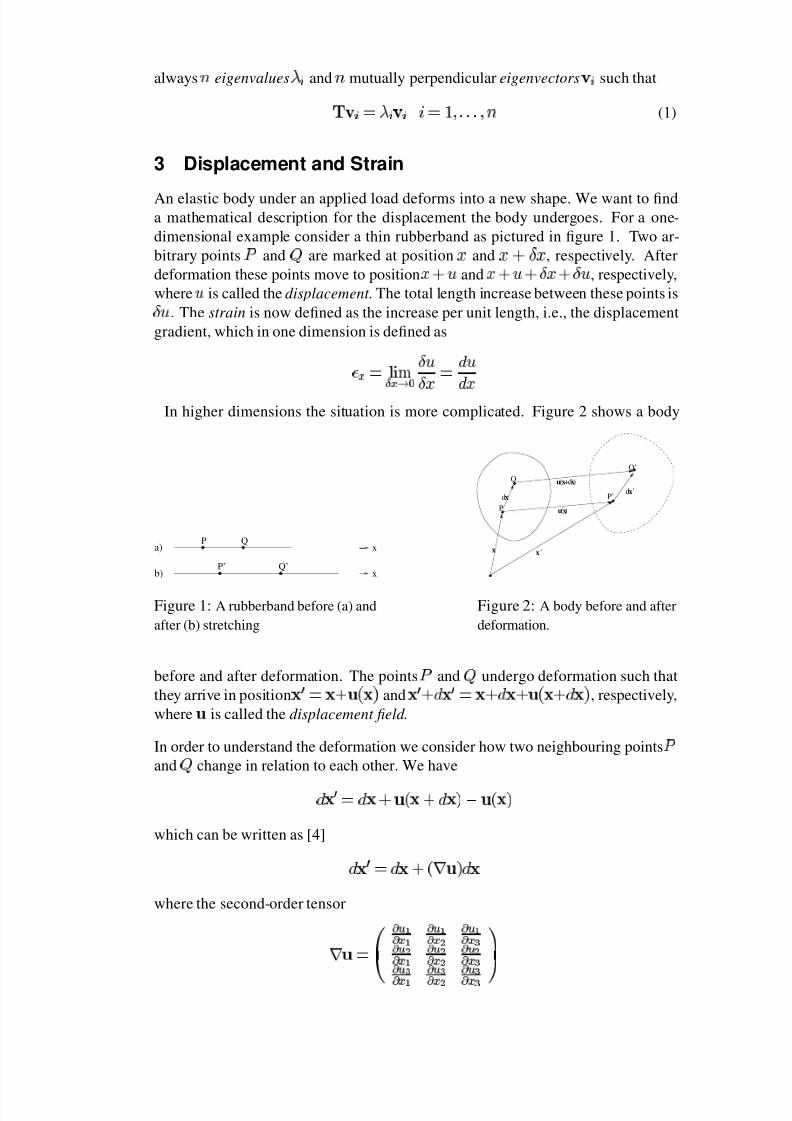
An elastic body under an applied load deforms into a new shape. We want to finda mathematical description for the displacement the body undergoes. For a one-

dimensional example consider a thin rubberband as pictured in figure 1. Two ar-

bitrary pointsP

andQ

are marked at positionx

andx + x

, respectively. After

deformation these points move to positionx + u

andx + u + x + u

, respectively,

whereu

is called the displacement . The total length increase between these points is

u

. The strain is now defined as the increase per unit length, i.e., the displacement

gradient, which in one dimension is defined as

x

= l i m

x ! 0

u

x

=

d u

d x

In higher dimensions the situation is more complicated. Figure 2 shows a body

b) x

a)P Q

P’ Q’

x

Figure 1: A rubberband before (a) and

after (b) stretching

x

x

P

Q (x

’

(x)

d

u )xd+

P’

x’

u

Q’

dx

Figure 2: A body before and after

deformation.

before and after deformation. The pointsP

andQ

undergo deformation such that

they arrive in positionx

0

= x + u x

andx

0

+ d x

0

= x + d x + u x + d x

, respectively,

whereu

is called the displacement field .

In order to understand the deformation we consider how two neighbouring pointsP

andQ

change in relation to each other. We have

d x

0

= d x + u x + d x , u x

which can be written as [4]

d x

0

= d x + r u d x

where the second-order tensor

r u =

0

B

@

@ u

1

@ x

1

@ u

1

@ x

2

@ u

1

@ x

3

@ u

2

@ x

1

@ u

2

@ x

2

@ u

2

@ x

3

@ u

3

@ x

1

@ u

3

@ x

2

@ u

3

@ x

3

1

C

A



is known as the displacement gradient .

It can be seen that if r u = 0

thend x

0

= d x

and the motion in the neighbourhood

of pointP

is that of a rigid body translation. The information about the material de-

formation aroundP

is contained inr u

. In order to define an entity which contains

information about deformation without rigid body rotation consider two material

vectorsd x

1

andd x

2

issuing from pointP

. Their dot product can be shown to be

([4])

d x

0

1

: d x

0

2

= d x

1

: d x

2

+ 2 d x

1

: E

d x

2

where the symmetric second-order tensor

E

=

1

2

r u + r u

T

+ r u

T

r u

is the Lagrangian strain tensor . Note that if E

= 0

the lengths and angles be-

tween the material vectorsd x

1

andd x

2

remain unchanged, i.e., the deformation

r u

around pointP

is an infinitesimal rigid body rotation. The components of E

areE

i j

=

1

2

@ u

i

@ x

j

+

@ u

j

@ x

i

+

@ u

k

@ x

i

@ u

k

@ x

j

!

For small deformations the displacement gradients@ u

i

= @ x

j

are small and the quadratic

term of E

can be neglected giving the strain tensor

i j

=

1

2

@ u

i

@ x

j

+

@ u

j

@ x

i

!

(2)

Lai et al. show [4] that for small values

i i

can be interpreted as the unit elongation

of a material element in thex

i

direction and2

i j

,i 6= j

can be interpreted as the

decrease in angle between two material vectors initially in thex

i

andx

j

directions.

Note that by definition the strain tensor

is symmetric. The eigenvectorsv

1

,v

2

,

andv

3

of

are the principal directions of the strain, i.e., the directions where there

is no shear strain. The eigenvalues

1

,

2

, and

3

are the principal strains and give

the unit elongations in the principal directions. The maximum, medium, and min-

imum eigenvalue are called the maximum, medium, and minimum principal strain,

respectively.

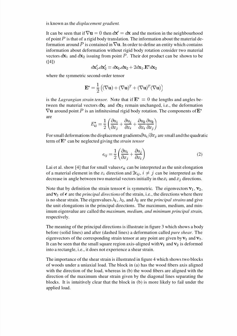
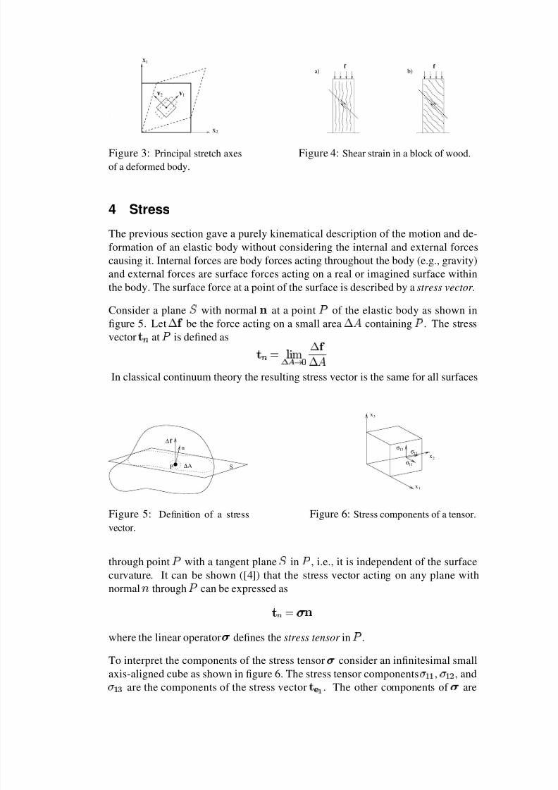
The meaning of the principal directions is illustrate in figure 3 which shows a body

before (solid lines) and after (dashed lines) a deformation called pure shear . The

eigenvectors of the corresponding strain tensor at any point are given byv

1

andv

2

.

It can be seen that the small square region axis-aligned withv

1

andv

2

is deformed

into a rectangle, i.e., it does not experience a shear strain.

The importance of the shear strain is illustrated in figure 4 which shows two blocks

of woods under a uniaxial load. The block in (a) has the wood fibers axis aligned

with the direction of the load, whereas in (b) the wood fibers are aligned with the

direction of the maximum shear strain given by the diagonal lines separating the

blocks. It is intuitively clear that the block in (b) is more likely to fail under the

applied load.



1x

2 1

x2

vv

Figure 3: Principal stretch axes

of a deformed body.

b)f f

a)

Figure 4: Shear strain in a block of wood.

4 Stress

The previous section gave a purely kinematical description of the motion and de-

formation of an elastic body without considering the internal and external forces

causing it. Internal forces are body forces acting throughout the body (e.g., gravity)

and external forces are surface forces acting on a real or imagined surface withinthe body. The surface force at a point of the surface is described by a stress vector .

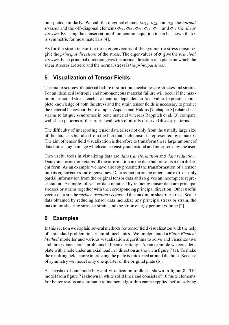
Consider a planeS

with normaln

at a pointP

of the elastic body as shown in

figure 5. Let f

be the force acting on a small area A

containingP

. The stress

vectort

n

atP

is defined as

t

n

= l i m

A ! 0

f

A

In classical continuum theory the resulting stress vector is the same for all surfaces

A∆P S

n

∆ f

Figure 5: Definition of a stress

vector.

11

σ12

σ13

x1

x2

x3

σ

Figure 6: Stress components of a tensor.

through pointP

with a tangent planeS

inP

, i.e., it is independent of the surface

curvature. It can be shown ([4]) that the stress vector acting on any plane with

normaln

throughP

can be expressed as

t

n

= n

where the linear operator

defines the stress tensor inP

.

To interpret the components of the stress tensor

consider an infinitesimal small

axis-aligned cube as shown in figure 6. The stress tensor components

1 1

,

1 2

, and

1 3

are the components of the stress vectort

e

1

. The other components of

are



interpreted similarly. We call the diagonal elements

1 1

,

2 2

, and

3 3

the normal

stresses and the off-diagonal elements

1 2

,

1 3

,

2 3

,

2 1

,

3 1

, and

3 2

the shear

stresses. By using the conservation of momentum equation it can be shown that

is symmetric for most materials [4].

As for the strain tensor the three eigenvectors of the symmetric stress tensor

give the principal directions of the stress. The eigenvalues of

give the principal

stresses. Each principal direction gives the normal direction of a plane on which the

shear stresses are zero and the normal stress is the principal stress.

5 Visualization of Tensor Fields

The major sources of material failure in structural mechanics are stresses and strains.

For an idealized isotropic and homogeneous material failure will occur if the max-

imum principal stress reaches a material dependent critical value. In practice com-

plete knowledge of both the stress and the strain tensor fields is necessary to predict

the material behaviour. For example, Aspden and Hukins [7, chapter 8] relate shear

strains to fatigue syndromes in bone material whereas Rappitch et al. [3] comparewall shear patterns of the arterial wall with clinically observed disease patterns.

The difficulty of interpreting tensor data arises not only from the usually large size

of the data sets but also from the fact that each tensor is represented by a matrix.

The aim of tensor field visualization is therefore to transform these large amount of

data into a single image which can be easily understood and interpreted by the user.

Two useful tools in visualizing data are data transformation and data reduction.

Data transformation retains all the information in the data but presents it in a differ-

ent form. As an example we have already presented the transformation of a tensor

into its eigenvectors and eigenvalues. Data reduction on the other hand extracts only

partial information from the original tensor data and so gives an incomplete repre-

sentation. Examples of vector data obtained by reducing tensor data are principal

stresses or strains together with the corresponding principal direction. Other useful

vector data are the surface traction vector and the maximum shearing stress. Scalar

data obtained by reducing tensor data includes: any principal stress or strain, the

maximum shearing stress or strain, and the strain energy per unit volume [2].

6 Examples

In this section we explain several methods for tensor field visualization with the helpof a standard problem in structural mechanics. We implemented a Finite Element

Method modeller and various visualization algorithms to solve and visualize two

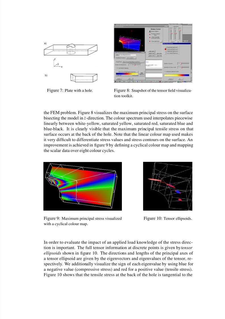
and three-dimensional problems in linear elasticity. An an example we consider a

plate with a hole under uniaxial load iny

direction as shown in figure 7 (a). To make

the resulting fields more interesting the plate is thickened around the hole. Because

of symmetry we model only one quarter of the original plate (b).

A snapshot of our modelling and visualization toolkit is shown in figure 8. The

model from figure 7 is shown in white solid lines and consists of 10 finite elements.

For better results an automatic refinement algorithm can be applied before solving



a)

b)

xy

z

Figure 7: Plate with a hole. Figure 8: Snapshot of the tensor field visualiza-

tion toolkit.

the FEM problem. Figure 8 visualizes the maximum principal stress on the surfacebisecting the model in

z

-direction. The colour spectrum used interpolates piecewise

linearly between white-yellow, saturated yellow, saturated red, saturated blue and

blue-black. It is clearly visible that the maximum principal tensile stress on that

surface occurs at the back of the hole. Note that the linear colour map used makes

it very difficult to differentiate stress values and stress contours on the surface. An

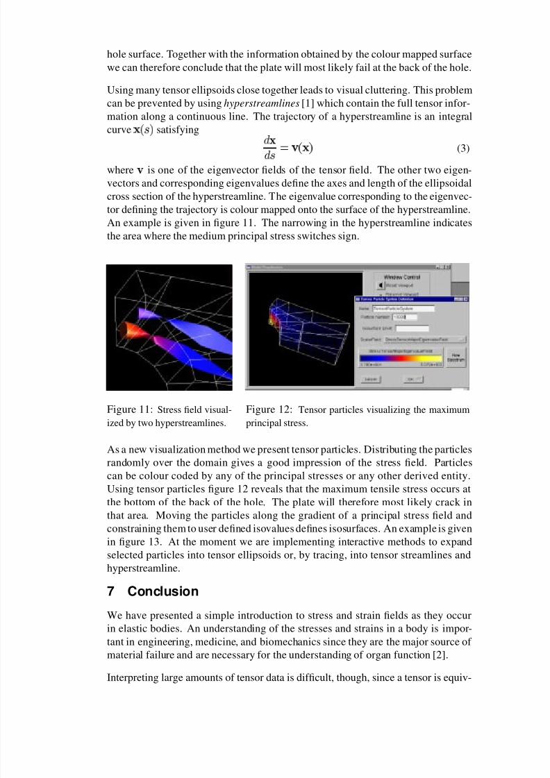
improvement is achieved in figure 9 by defining a cyclical colour map and mapping

the scalar data over eight colour cycles.

Figure 9: Maximum principal stress visualized

with a cyclical colour map.

Figure 10: Tensor ellipsoids.

In order to evaluate the impact of an applied load knowledge of the stress direc-

tion is important. The full tensor information at discrete points is given by tensor

ellipsoids shown in figure 10. The directions and lengths of the principal axes of

a tensor ellipsoid are given by the eigenvectors and eigenvalues of the tensor, re-

spectively. We additionally visualize the sign of each eigenvalue by using blue for

a negative value (compressive stress) and red for a positive value (tensile stress).

Figure 10 shows that the tensile stress at the back of the hole is tangential to the



hole surface. Together with the information obtained by the colour mapped surface

we can therefore conclude that the plate will most likely fail at the back of the hole.

Using many tensor ellipsoids close together leads to visual cluttering. This problem

can be prevented by using hyperstreamlines [1] which contain the full tensor infor-

mation along a continuous line. The trajectory of a hyperstreamline is an integral

curvex s

satisfyingd x

d s

= v x

(3)

wherev

is one of the eigenvector fields of the tensor field. The other two eigen-

vectors and corresponding eigenvalues define the axes and length of the ellipsoidal

cross section of the hyperstreamline. The eigenvalue corresponding to the eigenvec-

tor defining the trajectory is colour mapped onto the surface of the hyperstreamline.

An example is given in figure 11. The narrowing in the hyperstreamline indicates

the area where the medium principal stress switches sign.

Figure 11: Stress field visual-ized by two hyperstreamlines.

Figure 12: Tensor particles visualizing the maximumprincipal stress.

As a new visualization method we present tensor particles. Distributing the particles

randomly over the domain gives a good impression of the stress field. Particles

can be colour coded by any of the principal stresses or any other derived entity.

Using tensor particles figure 12 reveals that the maximum tensile stress occurs at

the bottom of the back of the hole. The plate will therefore most likely crack in

that area. Moving the particles along the gradient of a principal stress field and

constraining them to user defined isovalues defines isosurfaces. An example is given

in figure 13. At the moment we are implementing interactive methods to expandselected particles into tensor ellipsoids or, by tracing, into tensor streamlines and

hyperstreamline.

7 Conclusion

We have presented a simple introduction to stress and strain fields as they occur

in elastic bodies. An understanding of the stresses and strains in a body is impor-

tant in engineering, medicine, and biomechanics since they are the major source of

material failure and are necessary for the understanding of organ function [2].

Interpreting large amounts of tensor data is difficult, though, since a tensor is equiv-



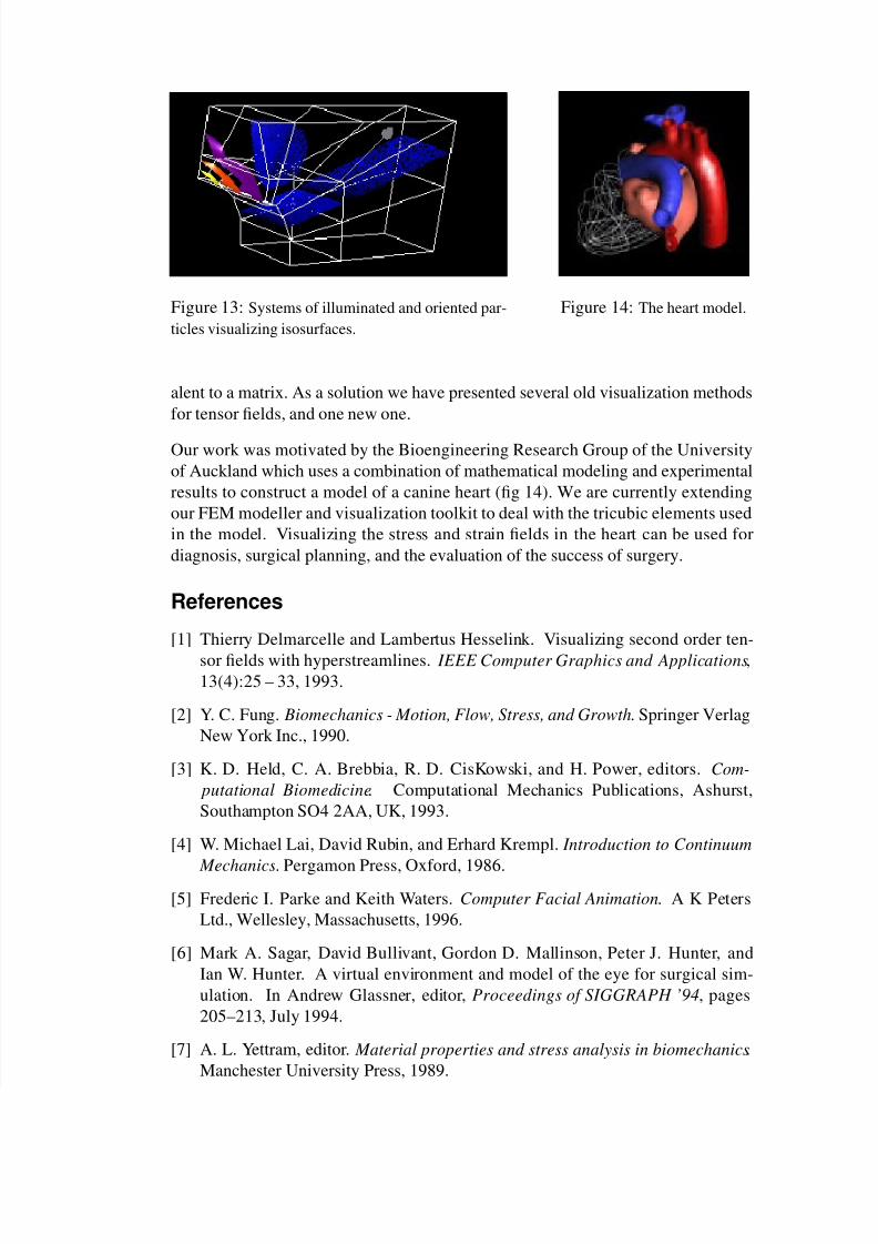
Figure 13: Systems of illuminated and oriented par-

ticles visualizing isosurfaces.

Figure 14: The heart model.

alent to a matrix. As a solution we have presented several old visualization methods

for tensor fields, and one new one.

Our work was motivated by the Bioengineering Research Group of the University

of Auckland which uses a combination of mathematical modeling and experimental

results to construct a model of a canine heart (fig 14). We are currently extending

our FEM modeller and visualization toolkit to deal with the tricubic elements used

in the model. Visualizing the stress and strain fields in the heart can be used for

diagnosis, surgical planning, and the evaluation of the success of surgery.

References

[1] Thierry Delmarcelle and Lambertus Hesselink. Visualizing second order ten-

sor fields with hyperstreamlines. IEEE Computer Graphics and Applications,

13(4):25 – 33, 1993.

[2] Y. C. Fung. Biomechanics - Motion, Flow, Stress, and Growth. Springer Verlag

New York Inc., 1990.

[3] K. D. Held, C. A. Brebbia, R. D. CisKowski, and H. Power, editors. Com-

putational Biomedicine. Computational Mechanics Publications, Ashurst,

Southampton SO4 2AA, UK, 1993.

[4] W. Michael Lai, David Rubin, and Erhard Krempl. Introduction to Continuum

Mechanics. Pergamon Press, Oxford, 1986.

[5] Frederic I. Parke and Keith Waters. Computer Facial Animation. A K Peters

Ltd., Wellesley, Massachusetts, 1996.

[6] Mark A. Sagar, David Bullivant, Gordon D. Mallinson, Peter J. Hunter, and

Ian W. Hunter. A virtual environment and model of the eye for surgical sim-

ulation. In Andrew Glassner, editor, Proceedings of SIGGRAPH ’94, pages

205–213, July 1994.

[7] A. L. Yettram, editor. Material properties and stress analysis in biomechanics.

Manchester University Press, 1989.

Stress Strain Paper

Documents

Transcript of Stress Strain Paper