Svensk Kärnbränslehantering ABSwedish Nuclear Fueland Waste Management Co

Box 250, SE-101 24 Stockholm Phone +46 8 459 84 00

R-09-14

CM

Gru

ppen

AB

, Bro

mm

a, 2

009

Stress strain flow curves for Cu-OFP

Rolf Sandström, Josefin Hallgren

Materials Science and Engineering

Royal Institute of Technology (KTH)

Gunnar Burman, Bodycote Materials Testing AB

April 2009

Tänd ett lager:

P, R eller TR.

Stress strain flow curves for Cu-OFP

Rolf Sandström, Josefin Hallgren

Materials Science and Engineering

Royal Institute of Technology (KTH)

Gunnar Burman, Bodycote Materials Testing AB

April 2009

ISSN 1402-3091

SKB Rapport R-09-14

Keywords: Copper, Stress strain curve, Tension, Compression, Creep.

This report concerns a study which was conducted for SKB. The conclusions and viewpoints presented in the report are those of the authors and do not necessarily coincide with those of the client.

A pdf version of this document can be downloaded from www.skb.se

3

Abstract

Stress strain curves of oxygen free copper alloyed with phosphorus Cu-OFP have been determined in compression and tension. The compression tests were performed at room temperature for strain rates between 10–5 and 10–3 1/s. The tests in tension covered the temperature range 20 to 175ºC for strain rates between 10–7 and 5×10–3 1/s. The results in compression and tension were close for similar strain rates.

A model for stress strain curves has been formulated using basic dislocation mechanisms. The model has been set up in such a way that fitting of parameters to the curves is avoided. By using a funda-mental creep model as a basis a direct relation to creep data has been established. The maximum engineering flow stress in tension is related to the creep stress giving the same strain rate.

The model reproduces the measured flow curves as function of temperature and strain rate in the inves-tigated interval. The model is suitable to use in finite-element computations of structures in Cu-OFP.

5

Contents

1 Introduction 7

2 Material and testing 9

3 Proof strength 11

4 Model for flow curves 134.1 Model 134.2 Comparison to experiments 154.3 Parameter values 19

5 Discussion 21

Conclusions 23

References 25

7

1 Introduction

The Swedish spent nuclear fuel is today stored in Clab, a central interim storage facility. The fuel will be stored there for 30 to 40 years and is then going to be moved to a final repository. The waste pack-age concept is referred to as KBS-3. The method involves the nuclear fuel waste being encapsulated in an insert made of iron with a surrounding copper canister. The iron insert provides the mechanical strength and the copper canister gives corrosion protection /1/. The material in the canister will be oxygen free copper alloyed with phosphorus, Cu-OFP. Between the copper canister and the insert there will be a gap of 1–2 mm to ensure that the inserts with holes for the fuel elements can safely be placed in the copper canisters /2/. The waste packages will be placed 500 m down in the bedrock sur-rounded by a buffer of bentonite clay. The clay reduces the transport of radionuclides into the rock in case of canister failure. The canister, the clay and the rock represent a multi barrier protective system.

The canisters will initially be exposed to a temperature close to 100ºC and an external pressure around 15 MPa from the surrounding bentonite and the groundwater. The external pressure and increased temperature will give rise to slow plastic deformation that gradually closes the gap between the canister and the insert. The maximum strain in the copper shells will be about 10% /3/, /4/.

In addition to corrosion performance the copper must show good ductility properties. To study the ductility behaviour, both traditional creep tests and tensile tests can be used. Slow strain rate tensile tests have been made before for cold worked copper /5/, but not for annealed Cu-OFP.

To describe the deformation in the copper canisters for nuclear waste, accurate data for creep and plastic deformation must be available. In this report tensile and compression tests of annealed oxygen free copper alloyed with phosphorus are analysed. Constitutive models for creep deformation have been dealt with elsewhere /6/. The aim of this study is to present tensile and compression tests of phosphorus alloyed pure copper. A model is also derived for stress strain flow curves to be used in elasto-plastic stress analysis.

9

2 Material and testing

The copper in the canisters will be in a soft condition, processed at high temperature without sub-sequent cold deformation. Only this soft condition is studied. The test material is copper with 45 to 60 ppm phosphorus. The composition is given in Table 2-1. Phosphorus gives copper higher creep ductility.

The first material is taken from an extruded tube with a diameter of 1,000 mm and a thickness of 50 mm. The tube has the designation 64-2-1 (T27). The tube was extruded at Wyman & Gordon from an ingot produced at Outokumpu, Pori. The second material is from a lid with the designation TX104. The lid was forged at Scana, Björneborg from an ingot produced at Norddeutsche Affineri AG. The analyses in Table 2-1 were made by the ingot producers.

The specimen geometries and test parameters are given in Table 2-2. Three test series are included. In the first set, tensile tests were performed at 20, 75, 125 and 175ºC for strain rates from 1×10–7 to 1×10–4 1/s. In the second and third sets tension and compression tests were carried out at room temperature at strain rates in the interval 5×10–5 to 5×10–3 1/s. The test series were performed at two laboratories, the first one at KTH and the second and third one at Bodycote. The tensile and compressive testing followed standard procedures (SS-EN 10002-1) and (DIN 50106), respectively except for chosen strain rates. In series 2 and 3, the strain rate was increased by a factor of five when 1% strain was reached but not in series 1. It is the final strain rate that is given in Table 2-2. The test series were performed in the following machines: Svenska Testprodukter 50 kN (series 1) and MTS DY36, UN-1370 (series 2 and 3).

Table 2-1. Composition of tested material, ppm.

Cu % Ag As Bi Cd Co Cr Fe H Mn Ni

Tube, Top 99.992 13.9 0.98 0.21 < 0.003 < 0.006 0.19 1.2 0.24 < 0.01 0.3

Tube, Bottom 99.993 13.6 1.05 0.21 < 0.003 < 0.006 0.2 1 0.37 < 0.01 0.3

Lid 99.992 13 1 < 1 < 1 < 1 < 1 2 – < 0.5 2

O P Pb S Sb Se Si Sn Te Zn

Tube, Top 1 60 0.22 5.8 0.49 0.46 < 0.2 0.051 0.24 < 0.01

Tube, Bottom 2.5 50 0.3 5.9 0.59 0.52 < 0.2 0.081 0.24 < 0.01

Lid 2 45–60 < 1 5 1 < 1 – < 0.5 < 1 < 1

Table 2-2. Specimen geometries and test conditions.

Test series

Material Specimen type Dimensions of gauge length

Test standard Test temper-atures, ºC

Strain rates, 1/s

1 Lid Tensile I Φ 10×50 mm – 20, 75, 125, 175

10–7, 10–6, 10–5, 10–4

2 Tube Tensile II Φ 10×56 mm SS-EN 10002-1* 20 5×10–5, 5×10–4, 5×10–3

3 Tube Compression Φ 10×25 mm DIN 50106* 20 5×10–5, 5×10–4, 5×10–3

*The strain rate was a factor of 5 lower below 1% strain.

11

3 Proof strength

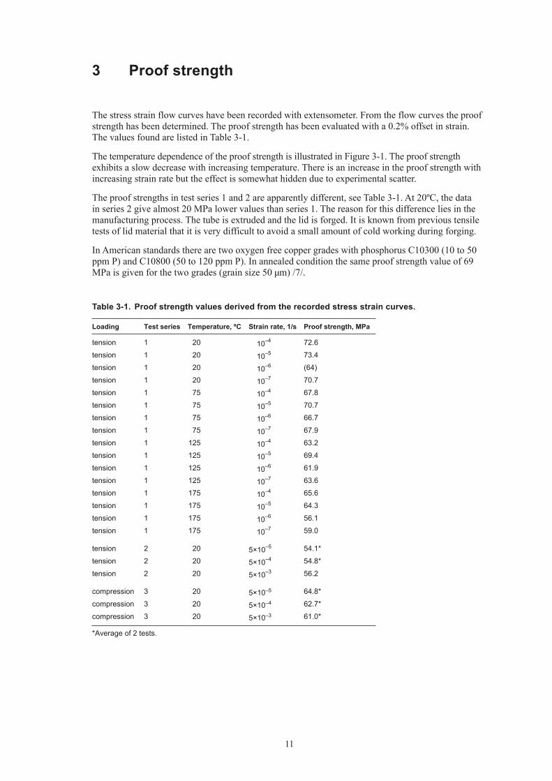
The stress strain flow curves have been recorded with extensometer. From the flow curves the proof strength has been determined. The proof strength has been evaluated with a 0.2% offset in strain. The values found are listed in Table 3-1.

The temperature dependence of the proof strength is illustrated in Figure 3-1. The proof strength exhibits a slow decrease with increasing temperature. There is an increase in the proof strength with increasing strain rate but the effect is somewhat hidden due to experimental scatter.

The proof strengths in test series 1 and 2 are apparently different, see Table 3-1. At 20ºC, the data in series 2 give almost 20 MPa lower values than series 1. The reason for this difference lies in the manufacturing process. The tube is extruded and the lid is forged. It is known from previous tensile tests of lid material that it is very difficult to avoid a small amount of cold working during forging.

In American standards there are two oxygen free copper grades with phosphorus C10300 (10 to 50 ppm P) and C10800 (50 to 120 ppm P). In annealed condition the same proof strength value of 69 MPa is given for the two grades (grain size 50 µm) /7/.

Table 3-1. Proof strength values derived from the recorded stress strain curves.

Loading Test series Temperature, ºC Strain rate, 1/s Proof strength, MPa

tension 1 20 10–4 72.6

tension 1 20 10–5 73.4

tension 1 20 10–6 (64)

tension 1 20 10–7 70.7

tension 1 75 10–4 67.8

tension 1 75 10–5 70.7

tension 1 75 10–6 66.7

tension 1 75 10–7 67.9

tension 1 125 10–4 63.2

tension 1 125 10–5 69.4

tension 1 125 10–6 61.9

tension 1 125 10–7 63.6

tension 1 175 10–4 65.6

tension 1 175 10–5 64.3

tension 1 175 10–6 56.1

tension 1 175 10–7 59.0

tension 2 20 5×10–5 54.1*

tension 2 20 5×10–4 54.8*

tension 2 20 5×10–3 56.2

compression 3 20 5×10–5 64.8*

compression 3 20 5×10–4 62.7*

compression 3 20 5×10–3 61.0*

*Average of 2 tests.

12

Figure 3-1. Proof strength versus temperature for test series 1. Values for four strain rates are shown from 1×10–7 to 1×10–4 1/s. The lines are model values given by eq. (7).

13

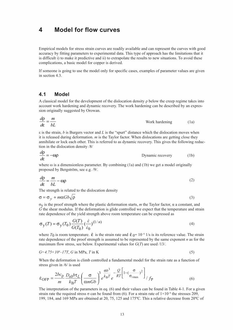
4 Model for flow curves

Empirical models for stress strain curves are readily available and can represent the curves with good accuracy by fitting parameters to experimental data. This type of approach has the limitations that it is difficult i) to make it predictive and ii) to extrapolate the results to new situations. To avoid these complications, a basic model for copper is derived.

If someone is going to use the model only for specific cases, examples of parameter values are given in section 4.3.

4.1 ModelA classical model for the development of the dislocation density ρ below the creep regime takes into account work hardening and dynamic recovery. The work hardening can be described by an expres-sion originally suggested by Orowan.

bLm

dd =

ερ

Work hardening (1a)

ε is the strain, b is Burgers vector and L is the “spurt” distance which the dislocation moves when it is released during deformation. m is the Taylor factor. When dislocations are getting close they annihilate or lock each other. This is referred to as dynamic recovery. This gives the following reduc-tion in the dislocation density /8/

ωρ−=ερdd Dynamic recovery (1b)

where ω is a dimensionless parameter. By combining (1a) and (1b) we get a model originally proposed by Bergström, see e.g. /9/.

ωρ−=ερ

bLm

dd (2)

The strength is related to the dislocation density

ρα+σ=σ Gbmy (3) σy is the proof strength where the plastic deformation starts, m the Taylor factor, α a constant, and G the shear modulus. If the deformation is glide controlled we expect that the temperature and strain rate dependence of the yield strength above room temperature can be expressed as

)/1(

000yy )(

)()()()( nεε

TGTGTT

&

&σ=σ (4)

where T0 is room temperature. ε is the strain rate and ε 0= 10–4 1/s is its reference value. The strain rate dependence of the proof strength is assumed to be represented by the same exponent n as for the maximum flow stress, see below. Experimental values for G(T) are used /13/.

G=4.75×104–17T, G in MPa, T in K (5)

When the deformation is climb controlled a fundamental model for the strain rate as a function of stress given in /6/ is used

P

)(13

B

0sOFP /

22

maxB

3

feemGbTk

bDmbc

iRTQ

Tkb

L

σ

σ−−σρ

αστ=ε& (6)

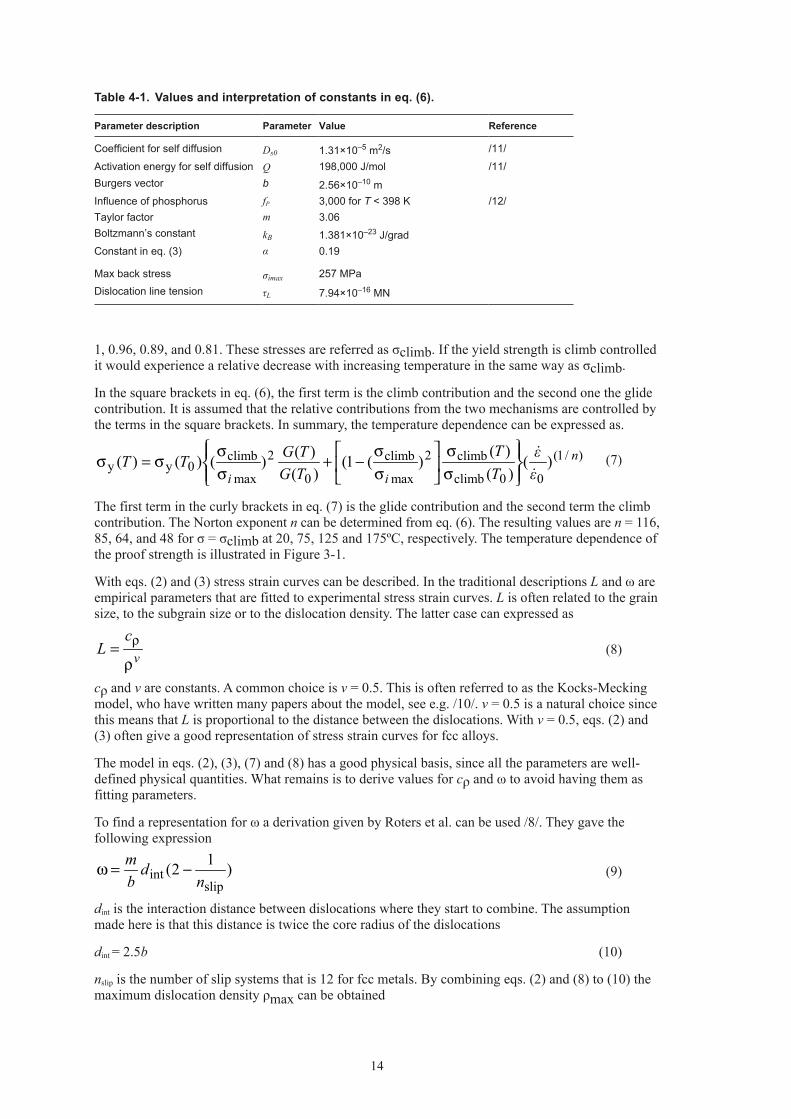
The interpretation of the parameters in eq. (6) and their values can be found in Table 4-1. For a given strain rate the required stress σ can be found from (6). For a strain rate of 1×10–4 the stresses 209, 199, 184, and 169 MPa are obtained at 20, 75, 125 and 175ºC. This a relative decrease from 20ºC of

14

1, 0.96, 0.89, and 0.81. These stresses are referred as σclimb. If the yield strength is climb controlled it would experience a relative decrease with increasing temperature in the same way as σclimb.

In the square brackets in eq. (6), the first term is the climb contribution and the second one the glide contribution. It is assumed that the relative contributions from the two mechanisms are controlled by the terms in the square brackets. In summary, the temperature dependence can be expressed as.

)/1(

00climb

climb2

max

climb

0

2

max

climb0yy )(

)()(

)(1()()()()()( n

ii εε

TT

TGTGTT

&

&

σσ

σσ

−+σσ

σ=σ (7)

The first term in the curly brackets in eq. (7) is the glide contribution and the second term the climb contribution. The Norton exponent n can be determined from eq. (6). The resulting values are n = 116, 85, 64, and 48 for σ = σclimb at 20, 75, 125 and 175ºC, respectively. The temperature dependence of the proof strength is illustrated in Figure 3-1.

With eqs. (2) and (3) stress strain curves can be described. In the traditional descriptions L and ω are empirical parameters that are fitted to experimental stress strain curves. L is often related to the grain size, to the subgrain size or to the dislocation density. The latter case can expressed as

vc

Lρ

= ρ (8)

cρ and v are constants. A common choice is v = 0.5. This is often referred to as the Kocks-Mecking model, who have written many papers about the model, see e.g. /10/. v = 0.5 is a natural choice since this means that L is proportional to the distance between the dislocations. With v = 0.5, eqs. (2) and (3) often give a good representation of stress strain curves for fcc alloys.

The model in eqs. (2), (3), (7) and (8) has a good physical basis, since all the parameters are well-defined physical quantities. What remains is to derive values for cρ and ω to avoid having them as fitting parameters.

To find a representation for ω a derivation given by Roters et al. can be used /8/. They gave the following expression

)12(slip

int nd

bm −=ω (9)

dint is the interaction distance between dislocations where they start to combine. The assumption made here is that this distance is twice the core radius of the dislocations

dint = 2.5b (10)

nslip is the number of slip systems that is 12 for fcc metals. By combining eqs. (2) and (8) to (10) the maximum dislocation density ρmax can be obtained

Table 4-1. Values and interpretation of constants in eq. (6).

Parameter description Parameter Value Reference

Coefficient for self diffusion Ds0 1.31×10–5 m2/s /11/

Activation energy for self diffusion Q 198,000 J/mol /11/Burgers vector b 2.56×10–10 mInfluence of phosphorus fP 3,000 for T < 398 K /12/Taylor factor m 3.06Boltzmann’s constant kB 1.381×10–23 J/gradConstant in eq. (3) α 0.19

Max back stress σimax 257 MPaDislocation line tension τL 7.94×10–16 MN

15

2max

))/12(2(1

slipnbc −=ρ

ρ (11)

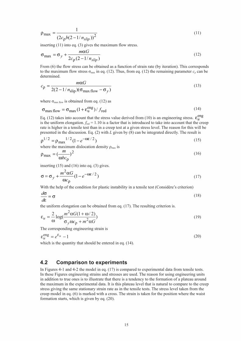
inserting (11) into eq. (3) gives the maximum flow stress.

)/12(2maxslip

y ncGm

−α+σ=σ

ρ (12)

From (6) the flow stress can be obtained as a function of strain rate (by iteration). This corresponds to the maximum flow stress σmax in eq. (12). Thus, from eq. (12) the remaining parameter cρ can be determined.

))(/12(2 flowmaxslip ynGmc

σ−σ−α=ρ (13)

where σmax flow is obtained from eq. (12) as

redengumaxflowmax /)1( fε+σ=σ (14)

Eq. (12) takes into account that the stress value derived from (10) is an engineering stress. enguε

is the uniform elongation. fred = 1.10 is a factor that is introduced to take into account that the creep rate is higher in a tensile test than in a creep test at a given stress level. The reason for this will be presented in the discussion. Eq. (2) with L given by (8) can be integrated directly. The result is )1( 2/2/1

max2/1 ωε−−ρ=ρ e (15)

where the maximum dislocation density ρmax is 2

max )(ρω

=ρbcm

(16)

inserting (15) and (16) into eq. (3) gives.

)1( 2/2

ωε−

ρ−

ωα+σ=σ ecGm

y (17)

With the help of the condition for plastic instability in a tensile test (Considère’s criterion)

σ=εσdd (18)

the uniform elongation can be obtained from eq. (17). The resulting criterion is.

))2/1(log(22

2

GmcGm

yu

α+ωσω+α

ω=ε

ρ (19)

The corresponding engineering strain is

1eng −=ε εueu (20)which is the quantity that should be entered in eq. (14).

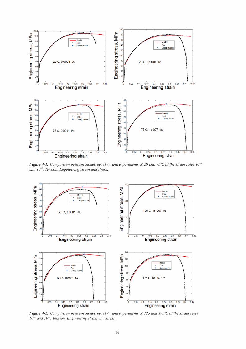
4.2 Comparison to experimentsIn Figures 4-1 and 4-2 the model in eq. (17) is compared to experimental data from tensile tests. In these Figures engineering strains and stresses are used. The reason for using engineering units in addition to true ones is to illustrate that there is a tendency to the formation of a plateau around the maximum in the experimental data. It is this plateau level that is natural to compare to the creep stress giving the same stationary strain rate as in the tensile tests. The stress level taken from the creep model in eq. (6) is marked with a cross. The strain is taken for the position where the waist formation starts, which is given by eq. (20).

16

Figure 4-1. Comparison between model, eq. (17), and experiments at 20 and 75ºC at the strain rates 10–4 and 10–7. Tension. Engineering strain and stress.

Figure 4-2. Comparison between model, eq. (17), and experiments at 125 and 175ºC at the strain rates 10–4 and 10–7. Tension. Engineering strain and stress.

17

As can been seen, the agreement between the model and the experiments is in general good. The model flow curve does not take into account the plastic instability at the maximum stress of the experimental curves. Comparison to the experimental data beyond this point is consequently meaningless.

The strain according Considère’s criterion is marked with a cross. It gives an acceptable estimate of the uniform elongation since it is close to the maximum in the experimental curves.

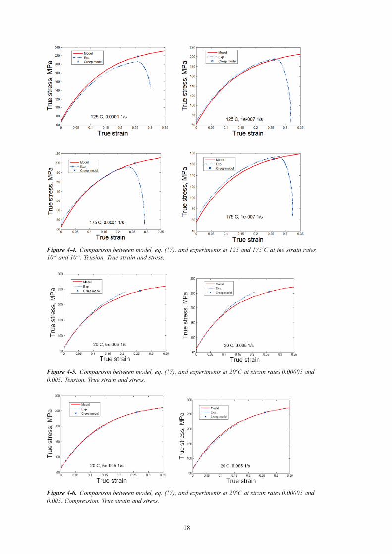
The corresponding Figures in true units are illustrated in Figures 4-3 and 4-4. In true units the flow curves have a simple exponential dependence of the strain. Curves from test series 2 are shown in Figure 4-5. For this series the stress was only recorded to 15% strain. There is some variation in the experimental curves. Some lie slightly above and some below the model curves. The close agreement between the model and the experiments in most cases is clearly seen. The exponential dependence of the stress with increasing strain in the model, cf. eq. (17), gives a good representation of the data. This applies to the whole investigated temperature range 20 to 175ºC and strain rates from 10–7 to 0.005 1/s.

The experimental results in Figures 4-1 to 4-5 are from tensile tests. In Figure 4-6 data from com-pression tests in series 3 are compared to the model. In fact, the compression and the tensile flow curves are quite close and the model can represent the compression results as well.

Figure 4-3. Comparison between model, eq. (17), and experiments at 20 and 75ºC at the strain rates 10–4 and 10–7. Tension. True strain and stress.

18

Figure 4-4. Comparison between model, eq. (17), and experiments at 125 and 175ºC at the strain rates 10–4 and 10–7. Tension. True strain and stress.

Figure 4-6. Comparison between model, eq. (17), and experiments at 20ºC at strain rates 0.00005 and 0.005. Compression. True strain and stress.

Figure 4-5. Comparison between model, eq. (17), and experiments at 20ºC at strain rates 0.00005 and 0.005. Tension. True strain and stress.

19

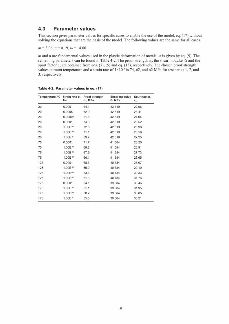
4.3 Parameter valuesThis section gives parameter values for specific cases to enable the use of the model, eq. (17) without solving the equations that are the basis of the model. The following values are the same for all cases.

m = 3.06, α = 0.19, ω = 14.66

m and α are fundamental values used in the plastic deformation of metals. ω is given by eq. (9). The remaining parameters can be found in Table 4-2. The proof strength σy, the shear modulus G and the spurt factor cρ are obtained from eqs. (7), (5) and eq. (13), respectively. The chosen proof strength values at room temperature and a strain rate of 1×10–4 is 74, 62, and 62 MPa for test series 1, 2, and 3, respectively.

Table 4-2. Parameter values in eq. (17).

Temperature, ºC Strain rate ε , 1/s

Proof strength σy, MPa

Shear modulus G, MPa

Spurt factor, cρ

20 0.005 64.1 42,519 22.9620 0.0005 62.9 42,519 23.4120 0.00005 61.6 42,519 24.0420 0.0001 74.0 42,519 25.5220 1.00E–05 72.5 42,519 25.9820 1.00E–06 71.1 42,519 26.5920 1.00E–07 69.7 42,519 27.2575 0.0001 71.7 41,584 26.2075 1.00E–05 69.8 41,584 26.9175 1.00E–06 67.9 41,584 27.7375 1.00E–07 66.1 41,584 28.65125 0.0001 68.3 40,734 28.07125 1.00E–05 65.9 40,734 29.10125 1.00E–06 63.6 40,734 30.33125 1.00E–07 61.3 40,734 31.76175 0.0001 64.1 39,884 30.46175 1.00E–05 61.1 39,884 31.95175 1.00E–06 58.2 39,884 33.85175 1.00E–07 55.5 39,884 36.21

21

5 Discussion

There is some variation between individual tests. This can be observed both for the proof strength and the remainder of the flow curves. It is well-known that mechanical testing of pure copper is sensitive to how specimens are machined, how they are set up in the test machine, etc. The variation in the test results is consequently no surprise.

A model for flow curves has been formulated. It is based on fundamental dislocation mechanisms. Two main assumptions are made. The first involves the efficient distance where dislocations interact during the recovery process. The distance is assumed to be twice the core radius of the dislocations. The second main assumption is that the level of the plateau in the engineering stress strain curves is related to the creep stress that gives the same strain rate. The dislocation barriers that are built up in the two types of tests can be expected to be somewhat different. In a strain controlled tests it is likely that the dislocation barriers are broken down more efficiently than in a stress controlled creep test. In the model it is assumed that the “stationary” stress level in the strain controlled test is 10% lower than the corresponding creep stress.

It is an important result that the creep and the tensile tests are closely related. It implies that the results can supplement each other. In addition, it helps identifying the deformation mechanisms involved. The creep model that has been used in the present paper is described in /6/. The creep model is based on a combination of climb and glide of dislocations. Thus, it is likely that the compression and tensile tests are controlled by the same mechanisms.

The model is used to represent stress strain flow curves in a fairly wide range. Temperatures from 20 to 175ºC and strain rates from 10–7 to 0.005 1/s are covered. It is apparent that the fit to data is equally good in all of this range. This confirms that the model can take into account the differences in temperatures and strain rates. Since the difference between compression and tension in the experi-ments is small, the model is applicable to both these types of loading.

23

Conclusions

Tensile and compression tests of oxygen free copper alloyed with phosphorus have been performed. To analyse the data a fundamental model for stress strain curves has been set up. The model is intended for finite-element calculations of structures in the material.

• Three test series gave proof strengths at room temperature and at a strain rate of 10–4 1/s of 74, 55 and 63 MPa, respectively. The first two series were performed in tension, the third one in compression. The reason for the higher yield strength in the first test series is that forged material was used, which has typically a small amount of cold work.

• The presented model for stress strain curves can describe the temperature, strain rate and strain dependences in the tests quite well. The range analysed is 20 to 175ºC and 10–7 to 0.005 1/s.

• Stress strain curves in compression were determined at room temperature and were found to be close to the values in tension, indicating that the same model can be applied in both loading cases.

• The model for the stress strain curve is based on an expression for the secondary creep rate. The creep stress that gives the same strain rate as in the tensile tests is used to determine the maximum engineering flow stress. In this way a direct relation between the creep and the constant strain rate tests has been established.

25

References

/1/ Kapsel för använt kärnbränsle, 2006. Tillverkning av kapselkomponenter. SKB R-06-03, Svensk Kärnbränslehantering AB.

/2/ Kapsel för använt kärnbränsle, 2006. Konstruktionsförutsättningar. SKB R-06-02, Svensk Kärnbränslehantering AB.

/3/ Jin L Z, Sandström R, 2009. Non-stationary creep simulation with a modified Armstrong-Frederick relation applied to copper canisters, Computer materials science, in press, doi:10.1016/j.commatsci.2009.03.017.

/4/ Jin L Z, Sandström R, 2009. Modified Armstrong-Frederick relation for handling back stresses in FEM computations, 2nd international ECCC conference. Creep & fracture in high temperature components – design & life assessment issues, Dübendorf, Switzerland.

/5/ Yao X X, Sandström R, 2000. Study of creep behaviour in P-doped copper with slow strain rate tensile tests. SKB TR-00-09, Svensk Kärnbränslehantering AB.

/6/ Sandström R, Andersson H C M, 2008. Creep in phosphorus alloyed copper during power-law breakdown, Journal of Nuclear Materials 372, 76–88.

/7/ ASM Handbook Volume 02, 1991. Properties and Selection: Nonferrous Alloys and Special-Purpose Materials, ASM.

/8/ Roters F, Raabe D, Gottstein G, 2000. Work hardening in heterogeneous alloys – a micro-structural approach based on three internal state variables, Acta mater. 48, 4181–4189.

/9/ Bergström Y, Hallen H, 1982. An improved dislocation model for the stress-strain behaviour of polycrystalline alpha-Fe, Materials Science and Engineering, 55, 49–61.

/10/ Mecking H, Kocks U F, 1981. Kinetics of flow and strain-hardening, Acta Metall. 29, 1865–1875.

/11/ Neumann G, Tölle V, Tuijn C, 1999. Monovacancies and divacancies in copper: Reanalysis of experimental data, Physica B: Condensed Matter 271, Issues 1-4, 21–27.

/12/ Sandström R, Andersson H C M, 2008. The effect of phosphorus on creep in copper, Journal of Nuclear Materials, 372, 66–75.

/13/ Raj S V, Langdon T G, 1989. Creep behavior of copper at intermediate temperatures-I. Mechanical characteristics, Acta Metall. 37, 843.