Stress analysis of polycrystalline thin films and surface...

topical reviews

J. Appl. Cryst. (2005). 38, 1–29 doi:10.1107/S0021889804029516 1

Journal of

AppliedCrystallography

ISSN 0021-8898

Received 14 April 2004

Accepted 12 November 2004

# 2005 International Union of Crystallography

Printed in Great Britain – all rights reserved

Stress analysis of polycrystalline thin films andsurface regions by X-ray diffraction

U. Welzel,a* J. Ligot,a P. Lamparter,a A. C. Vermeulenb and E. J. Mittemeijera

aMax Planck Institute for Metals Research, Heisenbergstr. 3, 70569 Stuttgart, Germany, andbPANalytical, Lelyweg 1, 7602 EA Almelo, The Netherlands. Correspondence e-mail:

[email protected]

The components of the macroscopic mechanical stress tensor of a stressed thin

film, coating, multilayer or the region near the surface of a bulk material can in

principle be determined by X-ray diffraction. The various analysis methods and

measurement strategies, in dependence on specimen and measurement

conditions, are summarized and evaluated in this paper. First, different X-ray

diffraction geometries (conventional or grazing incidence) are described. Then,

the case of macroscopically elastically isotropic, untextured specimens is

considered: from the simplest case of a uniaxial state of stress to the most

complicated case of a triaxial state of stress. The treatment is organized

according to the number of unknowns to be determined (i.e. the state of stress,

principal axes known or unknown), the use of one or several values of the

rotation angle ’ and the tilt angle of the sample, and one or multiple hkl

reflections. Next, the focus is on macroscopically elastically anisotropic (e.g.

textured) specimens. In this case, the use of diffraction (X-ray) elastic constants

is not possible. Instead, diffraction (X-ray) stress factors have to be used. On the

basis of examples, it is demonstrated that successful diffraction stress analysis is

only possible if an appropriate grain-interaction model is applied.

1. Introduction

In thin films and regions near the surface of bulk materials,

residual stresses are generally present (see, for example,

Hoffman, 1966, 1976; Windischmann, 1992; Machlin, 1995;

Proceedings of the International Conference on Residual

Stresses, Proceedings of the European Conference on Residual

Stresses). The analysis of the residual stress state is of great

technological importance because stresses can be beneficial or

detrimental with respect to, in particular, the mechanical

properties (see, for example, Hauk, 1997, x6 therein). As an

example, stress can result in cracking of a film in the case of

tensile stress, or buckling in the case of compressive stress. If,

on the other hand, a film or surface layer can be pre-stressed

during its production, a compressive pre-stress may prevent

cracking when stresses resulting from external forces occur

during service life.

Among a number of methods available for stress analysis,

X-ray diffraction methods employing the characteristic

radiation emitted from an X-ray tube or medium-energy

synchrotron radiation (E = 5–15 keV) are very suitable for the

analysis of films and surface layers. The rather limited pene-

tration depth of (such) X-rays in solid matter results in surface

sensitivity. X-ray diffraction methods allow a determination of

the full mechanical stress tensor of all crystalline phases;

furthermore, the analysis of stress gradients is feasible.

Moreover, useful additional information can be obtained as a

by-product of X-ray diffraction stress measurements: whereas

the stress analysis uses the shifts of diffraction lines, the

(integral) intensities of diffraction lines contain information

on the crystallographic texture (see, for example, Bunge,

1982), and the shapes and breadths of diffraction lines contain

information on the size (distribution) of diffracting domains

and the content of crystalline defects such as dislocations and

stacking faults (see, for example, Delhez et al., 1982).

In principle, no distinction exists between the analysis of

stress in bulk materials and in thin layers. However, dedicated

diffraction geometries for films much thinner than the X-ray

penetration depth have been developed in the past few years

and thin films are frequently mechanically elastically aniso-

tropic due to the occurrence of crystallographic texture and/or

direction-dependent grain interaction1 (Welzel & Mittemeijer,

2003). Thus, standard methods of analysis applicable to bulk

aggregates [e.g. the traditional sin2 analysis employing

diffraction (X-ray) elastic constants] may fail when applied to

the stress analysis of thin films (see, for example, van Leeuwen

et al., 1999; Leoni et al., 2001; Welzel et al., 2003; Welzel, Leoni

& Mittemeijer, 2004). New developments dedicated to the

stress analysis of thin films and surface layers are a focal point

of interest in this review paper.

1 The notion ‘direction-dependent grain interaction’ signifies that differentgrain-interaction assumptions prevail along different directions in thespecimen.

A selection of reviews on X-ray diffraction stress analysis in

the past 25 years is given in Table 1. Only reviews with a

general scope, i.e. reviews not only dedicated to a certain class

of materials (e.g. ceramics, metals or polymers), have been

included. The listing is not complete but embodies a repre-

sentative collection. Inspection of the existing literature shows

that earlier reviews are either incomplete or superficial, in

particular in view of the indicated new developments. A

practical systematization and a balanced presentation of the

determination of the state of stress for macroscopically elas-

tically isotropic versus anisotropic bodies is lacking. Further, a

review on stress analysis of thin films should at least mention

methods of analysis applicable to textured polycrystals, as

texture is met frequently in thin films. It is indispensable, in

this case, to at least mention the use of diffraction (X-ray)

stress factors and the use of the crystallite group method, and

yet previous reviews that focused on the case of thin films did

not deal with these aspects.

The present work reviews the various methods of (X-ray)

diffraction analysis of macroscopic mechanical stress states.

For this reason, methods for the analysis of local stresses down

to the submicrometre scale by microdiffraction employing

synchrotron radiation, a rapidly developing field of research

(see, for example, Tamura et al., 2003, and references therein),

have been excluded. These methods require dedicated

diffraction apparatus (e.g. white-beam synchrotron radiation,

two-dimensional detectors) as well as dedicated methods of

analysis. Further, the analysis of microstresses/strains from

diffraction line broadening has been excluded (see, for

example, Mittemeijer & Scardi, 2004). The purely technical

aspects (such as the selection of X-ray optics, the selection of

X-ray counters, etc.) of the stress measurement, as well as the

determination of the position of diffraction lines (i.e. the

maximum or centroid of a diffraction line), are not treated.

For details, the reader is referred to, for example, Hauk (1997,

xx2.04 and 2.05 therein). Measurement strategies for stress

analysis at fixed information depth are discussed, but the

calculation of stress depth profiles from such measurements

exceeds the scope of this paper and has been excluded (for an

example, see Somers & Mittemeijer, 1990).

Special attention is paid to the determination of stress in

thin films. Recipes are given that allow direct practical appli-

cation of traditional and new methods. The paper is organized

as follows. The theoretical, general equations for the stress

analysis of macroscopically elastically isotropic and aniso-

tropic polycrystals are presented in x2. The different diffrac-

tion geometries (modes of sample rotation, conventional and

grazing-incidence diffraction) are briefly described in x3. The

practical methods of stress analysis for macroscopically elas-

tically isotropic polycrystals have been gathered in x4. These

methods are tailored for specific states of stresses, in such a

way that they allow the direct determination of the stress

tensor components from simple linear regressions in plots of

measured lattice strains. The practical methods of stress

analysis for macroscopically elastically anisotropic specimens

(i.e. of specimens possessing crystallographic texture and/or

direction-dependent grain interaction) are dealt with in x5.

Different grain-interaction models, enabling the calculation

of diffraction (X-ray) elastic constants and diffraction (X-ray)

stress factors from single-crystal elastic data, are presented in

Appendix A.

2. Theoretical background

In the absence of external loads, stresses present in the sample

are called residual stresses. Three additive kinds of residual

topical reviews

2 U. Welzel et al. � Stress analysis J. Appl. Cryst. (2005). 38, 1–29

Table 1Review articles on diffraction stress analysis with a short description of the contents according to various categories.

Reference Focus Fundamentals Instrumentation

Analysis of

gradients

Elastically

quasi-isotropic

case

Elastically

anisotropic case

(case of texture) Comments

Noyan et al.

(1995)

Thin-film stress

analysis by X-ray

diffraction; poly-

crystalline and

epitaxial films

Origins of stress;

types of residual

stresses (macro

versus micro);

stress states of thin

films

Brief treatment of

traditional (Bragg–

Brentano,

Seeman–Bohlin)

and high-resolu-

tion diffract-

ometers;

microbeam

diffraction

Grazing/glancing-

incidence diffrac-

tion

Basic treatment – Also covered: stress

from curvature

measurements,

reflectometry for

determination of

film thickness and

composition

Eigenmann &

Macherauch

(1995)

Stress analysis by X-

ray diffraction;

poly- and single-

crystalline speci-

mens

Historical review;

types of residual

stresses (macro

versus micro)

Detailed treatment of

laboratory (Bragg–

Brentano) and

portable diffract-

ometers

– Full treatment; calcu-

lation of X-ray

elastic constants

– Sequence of four

publications in

German; introduc-

tion with historical

review

Hauk (1995) Stress analysis by X-

ray and neutron

diffraction; poly-

crystalline speci-

mens

Brief introduction Brief introduction Brief introduction Brief introduction Only mentioned; no

details

In German

Dolle (1979) Stress analysis by X-

ray diffraction;

polycrystalline

specimens

Brief introduction

and brief historical

review

– Effect of a stress

gradient on a

sin2 analysis isdiscussed

Full treatment; calcu-

lation of X-ray

elastic constants

Simplified treatment

(assuming a Reuss-

type grain interac-

tion)

stresses in a polycrystalline material are distinguished

according to their corresponding length scales (Macherauch et

al., 1973; see also Noyan et al., 1995):

�RS ¼ �RSI þ �

RSII þ �

RSIII ; ð1Þ

where �RSI represents the average of the residual stresses over

many grains. �RSII is defined as the difference between the

average of the residual stresses over a particular grain and �RSI .

�RSIII represents the deviation of the local stress �RS in a

particular grain from the average stress in the grain. In the

present work, only the determination of the macro-residual

stress �RSI is dealt with. For origins of residual stresses in thin

films, see e.g. the review by Windischmann (1992) and many

references therein.

2.1. Concept of diffraction stress analysis

The basic idea is sketched in Fig. 1, where it is assumed that

a polycrystalline specimen is subjected to a compressive stress

parallel to the surface. Due to the presence of stress, the lattice

spacing of the hkl lattice planes in a crystallite depends on the

orientation of the crystallite in the specimen with respect to

the specimen frame of reference. With X-ray diffraction

analysis, direction-dependent measurement of (elastic) lattice

strains is possible. Bragg’s law,

� ¼ 2dhkl sin �hkl; ð2Þ

relates the lattice spacing dhkl of the planes with Laue indices

hkl to the diffraction angle 2�hkl and the wavelength �. Note

that the lattice spacing is measured in the direction of the

diffraction vector. Usually the diffraction angle 2�hkl (a fixed

value for one reflection) is obtained from the position of the

maximum or centroid of the hkl diffraction line. Then it is

possible to calculate the elastic strain of the {hkl} planes from

"hkl¼ ðdhkl

ÿ dhkl0 Þ=dhkl

0 ; ð3Þ

where dhkl0 is the strain-free lattice spacing of the {hkl} lattice

planes. The direction of the strain measurement, i.e. the

direction of the diffraction vector, is usually identified by the

angles ’ and , where is the angle of inclination of the

specimen surface normal with respect to the diffraction vector

and ’ denotes the rotation of the specimen around the

specimen surface normal (see Fig. 2).

A diffraction line contains information on the elastic strain

of crystallites only for such crystallites which have their {hkl}

planes oriented perpendicular to the diffraction vector, i.e.

only the elastic strain of a subgroup of crystallites composing a

polycrystalline specimen is analysed in a lattice-strain

measurement. In general, the strain measured by X-ray

diffraction is not equal to the mechanical strain in the same

direction, characterized by (’, ), as the mechanical strain is

an average over all crystallites in the sample, whereas the

diffraction strain represents only a subgroup of the crystallites

composing the sample. Thus, it is of paramount importance in

diffraction stress analysis to distinguish diffraction averages,

e.g. the diffraction strain for a given reflection hkl in a given

direction, from the mechanical average strain in the same

direction.

Basic equations for the handling of tensorial quantities (like

strain and stress tensors) in the various appropriate frames of

reference, and the corresponding mechanical and diffraction

averages, also in the case of preferred orientation (texture),

are summarized in the following.

2.2. Frames of reference for diffraction stress analysis

The following Cartesian reference frames will be distin-

guished (see also Fig. 2).

The crystal reference frame (C): In general, a convention for

the definition of an orthonormal crystal system, such as that

given by Nye (1957) (for a detailed treatment, see also

Giacovazzo et al., 1998), has to be adopted. For cubic crystal

symmetry, the axes are chosen to coincide with the a, b and c

axes of the crystal lattice.

The specimen reference frame (S): The S3 axis is oriented

perpendicular to the specimen surface and the S1 and S2 axes

topical reviews

J. Appl. Cryst. (2005). 38, 1–29 U. Welzel et al. � Stress analysis 3

Figure 1Concept of diffraction stress analysis. When a polycrystal is subjected tostress (in this case a uniaxial compression parallel to the surface), thelattice spacing of the hkl lattice planes varies with the orientation of thelattice planes with respect to the loading direction. This direction-dependent lattice strain can be measured by X-ray diffraction. Thedirection of the strain measurement is the direction of the diffractionvector and is identified by the angles ’ and , where ’ is the rotationangle of the specimen about the specimen surface normal and is theinclination angle of the specimen surface normal with respect to thediffraction vector.

Figure 2Definition of, and relations between, the sample (S) and laboratory (L)reference frames.

lie in the surface plane. If a preferred direction within the

plane of the surface exists, e.g. the rolling direction in the case

of a rolled specimen, the S1 direction is usually oriented along

this preferred direction. A special specimen frame of refer-

ence is the principal reference frame (of the stress tensor) (P).

In this reference frame, only the following components of the

stress tensor are non-zero: �11, �22 and �33.

The laboratory reference frame (L): This frame is chosen in

such a way that the L3 axis coincides with the diffraction

vector. For ’ = = 0, the laboratory frame of reference

coincides with the specimen frame of reference.

In the following, a superscript [C, S (P) or L] is used to

indicate the reference frame adopted for the representation of

tensors. The absence of any superscript implies the validity of

an equation independent of the reference frame used for

tensor representation, but the same reference frame has to be

adopted for all tensors within the equation concerned. For the

relative orientation of the specimen and laboratory reference

frames with respect to each other, see Fig. 2.

Transformations of tensors (from one frame of reference to

another one) can be accomplished by suitable rotation

matrices describing the spatial relations between the frames of

reference concerned [for a general introduction to the use of

transformation matrices in the context of diffraction stress

analysis, see, for example, Noyan & Cohen (1987) and Hauk

(1997)].2.3. Crystallographic texture and the orientation distributionfunction (ODF)

The orientation of each crystallite in the S system can be

identified by three Euler angles. The convention of Roe &

Krigbaum (1964) in the definition of these angles will be

adopted and these angles will be called �, � and . The set of

Euler angles (�, �, ) can be associated with a vector g = (�, �,

) in the three-dimensional orientation (Euler) space G [for a

detailed treatment the reader is referred to e.g. Bunge (1982)].

In this way, each point in the orientation space represents a

possible orientation of the C reference frame (for the crys-

tallite concerned) with respect to the S reference frame. In the

absence of texture, it holds that the volume fraction of crys-

tallites having an orientation in the infinitesimal orientation

range d3g = sinð�Þ d� d� d around g is independent of g.

Texture can be quantified by introducing the so-called orien-

tation distribution function (ODF), f ð�; �; Þ, specifying the

volume fraction of crystallites having an orientation in the

infinitesimal orientation range d3g = sinð�Þ d� d� d around g:

dVðgÞ

V¼

f ðgÞ

8�2d3g ¼

f ð�; �; Þ

8�2sinð�Þ d� d� d ð4Þ

with R RG

R½f ðgÞ=8�2� d3g ¼ 1: ð5Þ

2.4. Tensor averages (mechanical and diffraction averages)

Mechanical and diffraction averages of stress and strain

tensors are usually calculated in Euler space G. In the

following, angular brackets h. . .i denote averages of a tensor

(e.g. the strain tensor) for all crystallites in the aggregate

considered, i.e. mechanical averages:

hi ¼1

8�2

R RG

RðgÞ f ðgÞ d3g

¼1

8�2

R2� ¼0

R��¼0

R2��¼0

ð�; �; Þ f ð�; �; Þ sinð�Þ d� dd� d :

ð6Þ

In equation (6), ð�; �; Þ has to be understood as an average

for all grains with a particular orientation in a specimen.

Braces f. . .g denote averages of a tensor (e.g. the strain

tensor) for diffracting crystallites only, i.e. diffraction averages.

A diffraction line contains data on only a subset of the crys-

tallites for which the diffracting planes are perpendicular to

the chosen measurement direction. A degree of freedom

occurs for the diffracting crystallites: the rotation around the

diffraction vector (denoted by the angle � in the following). In

a diffraction measurement, the subset of diffracting crystallites

is selected by hkl of the reflection considered and the orien-

tation of the diffraction vector with respect to the specimen

reference frame, which is indicated by the two angles ’ and .

These quantities, selecting the ensemble of crystallites for an

diffraction average, are attached to the corresponding average

as sub- (’, ) and superscripts (hkl):

f ghkl’; ¼

R 2�

0 ðhkl; �; ’; Þ f �ðhkl; �; ’; Þ d�R 2�

0 f �ðhkl; �; ’; Þ d�ð7Þ

f �ðhkl; �; ’; Þ is the representation of the ODF in terms of

the measurement parameters and the rotation angle �. The

ODF as defined in equation (4) cannot be directly used in

equation (7) in analogy to equation (6) since the angles �, ’, are not Euler angles representing a rotation of the C system

with respect to the S system (they provide the rotation of the

system L with respect to the system S). However, the values of

�, �, and thus f(�, �, ) at every � can be calculated from

hkl, �, ’ and , to be finally substituted for f �ðhkl; �; ’; Þ in

equation (7) [for a more detailed treatment of the necessary

transformations, see Leoni et al. (2001)]. Thus, the diffraction

strain "hkl’ can be calculated as the average strain f"L

33ghkl’ , i.e.

the strain parallel to the L3 axis:

"hkl’ ¼ f"

L33g

hkl’ ¼

R 2�

0 "L33ðhkl; �; ’; Þ f �ðhkl; �; ’; Þ d�R 2�

0 f �ðhkl; �; ’; Þ d�: ð8Þ

2.5. The basic equations of diffraction stress analysis

2.5.1. Elastically isotropic specimens. The simplest

specimen for diffraction stress analysis is a polycrystal

composed of (individually) elastically isotropic crystallites.

The basic principle of the method will be discussed for such a

specimen first, before the more complicated effects of single-

crystal elastic anisotropy, in combination with direction-

dependent grain interaction (cf. Appendix A) and texture, are

introduced.

topical reviews


For a polycrystal composed of elastically isotropic crystal-

lites, Hooke’s law relating the mechanical strain to the

mechanical stress tensor reads (see, for example, Meyers &

Chawla, 1984):

h"Siji ¼ SS

ijklh�Skli ¼ SC

ijklh�Skli

¼ S1�ij�kl þ12 S2

12 �ik�jl þ �il�jk

ÿ �� h�S

kli: ð9Þ

Note that the Einstein convention, i.e. summation over indices

appearing twice in a formula, is adopted throughout the paper.

SSijkl is the compliance tensor of the body referred to the

specimen reference frame and can be equated to SC, as the

individual crystallites are elastically isotropic (i.e. all crystal-

lites present identical elastic properties in any arbitrary frame

of reference). S1 and 12 S2 are the only independent compo-

nents of SC. Equation (9) holds for the macroscopic body, but

it also holds, in the case considered, for every crystallite in the

aggregate and thus also for the strain probed by X-ray

diffraction. Only in this case, all averages of tensors are equal

to the corresponding tensors of the individual crystallites; thus

all braces (for diffraction averages) and brackets (for

mechanical averages) could be skipped. The elastic constants

S1 and 12 S2 can be related to Young’s modulus E and Poisson’s

ratio � of the body:

S1 ¼ ÿ�=E ð10Þ

and

12 S2 ¼ ð1þ �Þ=E: ð11Þ

The elastic strain "hkl’ measured by X-ray diffraction is

obtained from equation (8). In this particular case, no aver-

aging is necessary as the strain tensor is identical for all

crystallites:

"hkl’ ¼ f"

L33g

hkl’ ¼ "

L33 ¼ h"

L33i: ð12Þ

h"L33i can be calculated from the strain tensor in the specimen

frame of reference, "S, and the unit vector, mS, in the direction

of the diffraction vector as expressed in the specimen frame of

reference as follows:

"hkl’ ¼ h"

L33i ¼ mS

i h"Sijim

Sj

¼ h"S11i cos2 ’ sin2 þ h"S

22i sin2 ’ sin2 þ h"S33i cos2

þ h"S12i sin 2’ð Þ sin2 þ h"S

13i cos ’ sin 2 ð Þ

þ h"S23i sin ’ sin 2 ð Þ; ð13Þ

where

mS¼

sin cos ’sin sin ’cos

0@ 1A: ð14Þ

By substitution of h"Siji in equation (13) using equation (9), the

so-called sin2 law, relating the diffraction strain to the

components of the mechanical stress tensor expressed in the

specimen frame of reference, follows in a straightforward

manner:

"hkl’ ¼

12 S2 sin2

�h�S

11i cos2 ’þ h�S12i sin 2’ð Þ þ h�S

22i sin2 ’�

þ 12 S2

�h�S

13i cos ’ sin 2 ð Þ þ h�S23i sin ’ sin 2 ð Þ

þ h�S33i cos2

�þ S1 h�

S11i þ h�

S22i þ h�

S33i

ÿ �: ð15Þ

Equation (15) holds for the diffraction strain, "hkl’ , as well as

for the mechanical strain, h"L33i. Note that, for a polycrystalline

aggregate, subjected to a homogeneous stress field and

consisting of elastically isotropic crystallites, equation (15)

holds also in the presence of crystallographic texture and/or

direction-dependent grain interaction.

The name of equation (15), ‘sin2 law’ (first introduced by

Macherauch & Muller, 1961), stems from the proportionality

of the measured strain to sin2 if the P frame of reference has

been adopted for the specimen frame of reference (principal

state of stress; all stress tensor components �Pij are zero for

i 6¼ j). A plot of the measured strain versus sin2 yields a

straight line (for constant ’) and the components of the stress

tensor can be extracted from the slopes of straight lines for

various ’. For stress analysis on the basis of the sin2 law

[equation (15)] in the presence of shear stresses, i.e. the

orientation of the P frame of reference is unknown, the reader

is referred to x4.

2.5.2. Macroscopically elastically isotropic and anisotropicspecimens. In practice, polycrystals composed of elastically

isotropic crystallites are seldomly met (tungsten is an example

of an elastically isotropic material). In a polycrystal composed

of elastically anisotropic crystallites, stresses and strains vary

over the (crystallographically) differently oriented crystallites

in the specimen, in contrast with a polycrystal composed of

elastically isotropic crystallites, where stresses and strains are

equal for all differently oriented crystallites. In the presence of

this intrinsic elastic anisotropy, the distribution of stresses and

strains that occurs is the result of the elastic grain interaction

(see Appendix A).

Even if the individual crystallites of a polycrystal are elas-

tically anisotropic, the whole body can still be macroscopically

elastically isotropic, which in the following is called quasi-

isotropic. This is the case if crystallographic texture does not

occur and if the grain interaction is isotropic (i.e. direction-

dependent grain interaction does not occur). Otherwise, the

body is macroscopically elastically anisotropic. These two

cases, i.e. macroscopic elastic isotropy (quasi-isotropy) and

macroscopic elastic anisotropy, have to be considered sepa-

rately for diffraction stress analysis.

It can be shown by exploiting the symmetries of the elastic

properties of subgroups of grains as selected by a diffraction

experiment that the concept of diffraction (X-ray) elastic

constants (XEC) holds for quasi-isotropic specimens, whereas

the concept of diffraction (X-ray) stress factors (XSF) has to

be used for elastically anisotropic specimens (Welzel &

Mittemeijer, 2003; see also Stickforth, 1966).

In the case of quasi-isotropic specimens, a sin2 law is

obtained, which differs from the sin2 law for elastically

isotropic specimens [equation (15)] only with respect to the

elastic constants S1 and 12 S2, which have to be replaced by so-

topical reviews


called hkl-dependent diffraction (X-ray) elastic constants Shkl1

and 12 Shkl

2 :

"hkl’ ¼ f"

L33g

hkl’

¼ 12 Shkl

2 sin2 �h�S

11i cos2 ’þ h�S12i sin 2’ð Þ þ h�S

22i sin2 ’�

þ 12 Shkl

2

�h�S

13i cos ’ sin 2 ð Þ þ h�S23i sin ’ sin 2 ð Þ

þ h�S33i cos2

�þ Shkl

1 h�S11i þ h�

S22i þ h�

S33i

ÿ �: ð16Þ

Note that according to the right-hand side of equation (16), in

contrast with equation (15), the diffraction strain now depends

on the reflection hkl. Stresses/strains of individual crystallites

are not equal to the corresponding mechanical averages. Thus

averaging brackets and averaging braces have to be used.

The modifications of equation (15) necessary to obtain

equation (16) were invented on an empirical basis: about ten

years after the first strain measurements by means of X-ray

diffraction, Moller & Barbers (1935) obtained experimental

results indicating that mechanical elastic constants [i.e. equa-

tion (15)] cannot be used for the stress analysis of polycrystals

composed of elastically anisotropic crystallites, i.e. diffraction

strains differ from mechanical strains due to the intrinsic

elastic anisotropy. Diffraction (X-ray) elastic constants were

eventually proposed on an empirical basis by Moller & Martin

(1939) (see also Bollenrath et al., 1941). For the special cases

of the Voigt grain-interaction model (Voigt, 1910) and the

Reuss grain-interaction model (Reuss, 1929), it was demon-

strated that such XECs can be applied (Moller & Martin,

1939).

At that time, the stress analysis was based on the back-

reflection technique involving X-ray sensitive films. The use of

diffractometers for stress analysis and the notion ‘sin2 method’ for an analysis based on equation (16) was estab-

lished in the 1950s (Macherauch & Muller, 1961; see also

Hauk, 1952; Christenson & Rowland, 1953). The analysis was

limited to a principal stress state; a generalization to a general

stress state was performed by Evenschor & Hauk (1975). A

general proof of the validity of equation (16) for any quasi-

isotropic polycrystal, independent of the type of grain inter-

action, was not given until some decades later by Stickforth

(1966).

In the case of macroscopically elastically anisotropic speci-

mens (i.e. in the presence of direction-dependent grain inter-

action and/or crystallographic texture, cf. x5.1), the so-called

X-ray stress factors (XSF) have to be employed for diffraction

stress analysis (see, for example, Hauk, 1997, and, in parti-

cular, Welzel & Mittemeijer, 2003):

f"L33g

hkl’ ¼ Fijð’; ; hklÞh�S

iji: ð17Þ

Experimentally, it was found (for a comprehensive review, see,

for example, Hauk, 1997) that non-linear sin2 plots are

generally observed for textured materials, even for the case of

a principal state of stress. Thus, the use of equation (16) for the

diffraction stress analysis is not possible, as equation (16)

indicates a linear dependence of the diffraction strain on sin2 (in the absence of shear stresses).

The pioneering work on the diffraction stress analysis of

macroscopically elastically anisotropic specimens was

performed by Dolle & Hauk (1978, 1979) for the case of

crystallographic texture and by van Leeuwen et al. (1999) for

the case of direction-dependent grain interaction, and by

Leoni et al. (2001) for the simultaneous occurrence of direc-

tion-dependent grain interaction and crystallographic texture.

The theoretical equations that can be used for crystal-

lographically textured polycrystals were originally given, as in

the quasi-isotropic case discussed directly above, by an

elaboration of a particular model for grain interaction, namely

the Reuss model, and in this context the stress factors

Fkl( , ’, hkl) were introduced (Dolle & Hauk, 1978, 1979). A

general proof of the validity of equation (17) for any macro-

scopically elastically anisotropic polycrystal, independent of

the type of grain interaction, was given recently by Welzel &

Mittemeijer (2003).

Note that Fij( , ’, hkl) has no superscript for indicating a

reference frame: Fij( , ’, hkl) is not a representation of a

tensor and thus no reference frame has to be indicated.

The evaluation of the diffraction (X-ray) elastic constants

Shkl1 and 1

2 Shkl2 and the diffraction (X-ray) stress factors

Fij( , ’, hkl) can be accomplished either by measurement, by

applying a known load stress to a specimen under simulta-

neous lattice strain measurement, or by calculation starting

from single-crystal elastic constants by adopting a suitable

grain-interaction model (see Appendix A).

A schematic diagram on the use of the two basic formulae,

equations (16) and (17), with reference to the structure of the

specimen and its elastic properties, is presented in Fig. 3.

topical reviews


Figure 3Schematic diagram of different situations in the field of diffraction stressanalysis depending on the structure of the specimen and the elasticproperties of the material composing the specimen (the cases in dashedboxes are not treated in the present paper).

3. Diffraction geometry

With conventional X-ray diffraction the variation of the angle

, defining the measurement direction with respect to the

sample surface normal, by tilting the specimen, is accom-

panied by a variation of the angle of incidence � and thus also

of the effective penetration depth of the X-ray beam in the

investigated sample. In the case of thin-film analysis,

depending on the film thickness and on the X-ray radiation

used, the X-rays may penetrate throughout the film into the

underlying substrate material. Thus the diffraction peaks of

the film and of the substrate can overlap and/or the signal-to-

background ratio for diffraction peaks of the film can become

very low, both effects hindering the quantitative evaluation of

the diffraction profile. Two solutions to this problem have

been employed: (i) the diffraction contribution of the

substrate using a separate measurement of the uncovered

substrate is removed, provided that no changes of the

substrate peaks due to the layer deposition occur [apart from

absorption (see, for example, Kamminga, Delhez et al., 2000)];

(ii) by keeping the effective penetration depth of the X-ray

beam small, the contribution of the substrate is reduced (see,

for example, van Acker et al., 1994).

The dependence of the beam penetration, as expressed by

the information depth [for definitions of various measures of

information depth, see Delhez et al. (1987)], on the angle of

incidence is utilized by dedicated methods (grazing-incidence

method and scattering vector method; see x3.2) to analyse the

stress at a fixed depth and thus to allow the determination of

stress profiles in films or near-surface regions of bulk mate-

rials.

A measure for the average information depth (for an

‘infinitely’ thick sample) is the so-called 1/e penetration depth,

�. It is the centre of gravity of the distribution of measured

diffracted intensity versus depth; about 63% of the diffracted

intensity originates from a volume confined by depth � below

the sample surface. � is given by

� ¼ sin � sin �=�ðsin �þ sin �Þ; ð18Þ

where � and � denote the angle of incidence and exit,

respectively, of the X-ray beam with respect to the sample

surface, and � is the effective linear absorption coefficient of

the material depending on the radiation used.

First, measurement methods which do not take care of the

variation of the penetration depth during the measurement

are discussed in x3.1. x3.2 focuses on grazing-incidence

methods, where the penetration depth can be controlled by a

proper choice of the instrumental angles.

3.1. Conventional X-ray diffraction

With the conventional diffraction geometry, no measures

are taken to control the penetration depth of the X-rays in the

sample by a defined angle of incidence, �, and/or of exit, �.

The rotation angles of the instrument are used only to bring

{hkl} planes, which are oriented in a certain way in the sample,

into diffraction condition, i.e. to align the normal of the {hkl}

planes parallel to the diffraction vector (L3 axis of the

laboratory system L; see Fig. 2).

In the following, the different angles required for the

description of diffraction geometries are defined. The angles ’and , describing the orientation of the normal of {hkl} planes

with respect to the specimen system S (see x2, Fig. 2) in the

sin2 formulae [see equations (16) and (17)] and the rotation

angles �, ! and � of the instrument, describing the orientation

of the sample with respect to the laboratory system L (see Fig.

4), have to be distinguished.

The instrumental angles are as follows.

2� = diffraction angle, set by the detector position. In the

following the angle � is strictly used as the Bragg angle (half of

the diffraction angle, i.e. angle between the incident beam and

crystallographic planes in diffraction condition) and not as the

angle between the incident beam and the sample surface.

� = rotation around the normal of the plate of the sample

stage. Usually the sample is mounted on the stage such that

the � axis and the ’ axis are parallel and the two rotation

angles are then simply related by a constant (rotational) offset.

! = angle of rotation of the sample around an axis

perpendicular to the diffraction plane, i.e. parallel to the 2�axis and perpendicular to the � axis. For symmetric diffraction

topical reviews


Figure 4Definition of the various angles required to describe the diffractiongeometries and variation of the angle using (a) the ! mode (shown for < 0) or (b) the � mode. L3 is the diffraction vector, S3 is the surfacenormal.

(Bragg–Brentano) condition: ! = � and (in addition) for � = 0:

� = !.

� = angle of rotation of the sample around an axis defined

by the intersection of the diffraction plane and the sample

surface (plate of the sample stage), i.e. perpendicular to the !axis and the 2� axis.

Confusion can be (but often is not) avoided if the angles !and � are not intermixed with the angles � and , respectively

(note that the term ‘2�/� scan’ is misleading and it should be

replaced by the term ‘2�/! scan’ ).

Diffraction planes {hkl} with a specific orientation ’ and in the specimen system S can be selected by setting of the

instrumental angles 2�, �, ! and �. The possibility to set an

angle either by ! or by � (or a combination of both) leads to

the distinction between the ! mode and the �mode in a stress

measurement (where the scan over the diffraction peak at

fixed is in both cases performed by a 2�/! scan).

3.1.1. x mode, v = 0 (Fig. 4a). Variation of ! [at fixed � =

�hkl; cf. equation (2)] provides a variation of the inclination of the measured {hkl} planes with respect to the sample

normal according to = ! ÿ � (the opposite convention = �ÿ ! is also found in the literature; however, note that, if the

polar angles ’ and are defined to specify the measuring

direction in the sample coordinate system, is always posi-

tive). Because of � = 0, the angle � of incidence is directly

given by the angle !; the exit angle is � = 2�ÿ ! = �ÿ . With

the ! mode only a restricted range of | | < � is accessible (the

limit is given by the position where the incident or the

diffracted beam is parallel to the sample surface).

Inserting � = � + and � = � ÿ into equation (18), the

penetration depth in terms of the two angles � and is

obtained:

�! ¼sin2 � ÿ sin2

2� sin � cos ð ¼ !ÿ �Þ: ð19Þ

3.1.2. v mode (w mode), x = h (Fig. 4b). For � mode, the

angle � is the same as the angle (therefore it is often also

called mode; another name is side-inclination method).

Variation of � (at fixed � = �hkl) provides a variation of the

inclination of the measured {hkl} planes with respect to the

sample normal. The true angle � of incidence (equal to the

angle of exit �) is given by

sin � ¼ sin �ð Þ ¼ sin! cos�: ð20Þ

From equations (18) and (20) the penetration depth in terms

of the two angles � and is obtained:

�� ¼sin �

2�cos ¼ �ð Þ: ð21Þ

Note that the rotation angle ’ describing the measurement

direction within the plane of the sample differs by 90� for the �and ! modes.

The errors in measured peak positions 2�hkl due to non-

ideal beam optics and to misalignment are different for the �mode and the ! mode. In particular, with the ! mode the

defocusing error is different for positive (! > �) and negative

(! < �) tilts of the sample. For corrections for non-ideal beam

optics, see Noyan & Cohen (1987) (and references therein)

and Vermeulen & Houtman (2000).

3.1.3. Combined x/v mode. For a tilt of the sample around

both the ! axis and the � axis simultaneously, the values of the

various angles are not obvious but can be calculated by

expressing the directions of the incoming beam, the diffracted

beam and the diffraction vector in the S system, employing

appropriate rotation matrices. The measuring direction (’, )

in the S system is given by

’ ¼ �þ arctanÿ sin�

tan !ÿ �ð Þ

� �ð22Þ

and

¼!ÿ �

!ÿ �j jarccos cos� cos !ÿ �ð Þ½ �: ð23Þ

The angle of incidence, �, is given by equation (20) and the

exit angle of the diffracted beam with respect to the sample

surface, �, is given by

sin � ¼ sin 2� ÿ !ð Þ cos�: ð24Þ

With conventional X-ray diffraction, whatever the mode

considered, all combinations of the instrumental angles �, !, �and � are possible, because the orientation of the specimen

and the diffraction angle � can be chosen independently (in

contrast to the grazing-incidence methods; see below).

However, the choice of the reference position of the sample

(i.e. the choice of the orientation of the axis, ! or � mode,

and the direction ’ = 0� with respect to the sample geometry)

defines the frame of reference for the tensor components h"Siji

and h�Siji.

3.2. Grazing-incidence X-ray diffraction

For very thin surface-adjacent layers, the X-ray diffraction

measurement of specimen properties, like residual stress and

crystallite orientation distribution, is possible by using small

angles of incidence [introduced as the low incident-beam

angle diffraction method (LIBAD) by van Acker et al. (1994)].

The grazing-incidence X-ray diffraction (GIXD) method

(using so-called in-plane diffraction geometry where the

diffraction vector is parallel to the sample surface) was

originally developed by Marra et al. (1979). Using small angles

� of incidence the effective sampling volume is confined to a

relatively small volume adjacent to the surface of the sample

yielding higher diffracted intensities from this volume than

with conventional X-ray diffraction methods. Sometimes in

the literature the terms ‘grazing-incidence XRD’ and

‘glancing-incidence XRD’ are used (see, for example, Noyan et

al., 1995) to distinguish, respectively, between angles � of

incidence very close to the critical angle for total external

reflection (some tenths of a degree), where the penetration

depth is of the order of a few nanometres only, and angles � of

incidence of a few degrees, where the penetration depth is of

the order of a few micrometres. Examples are shown in Fig. 5.

In the following the term grazing-incidence X-ray diffraction

topical reviews


(GIXD) is used for geometries involving both (overlapping)

ranges of angles of incidence mentioned above.

The GIXD method for stress analysis is useful in two cases:

(i) to restrict the effective penetration depth to a defined small

value when the stress state at (close to) the surface of a body

has to be determined or when stress analyses have to be

performed for very thin films for which problems of overlap

with substrate peaks can occur; (ii) to determine stress

gradients from diffraction measurements at different effective

penetration depths by varying the angle � of incidence or the

wavelength. If the angle � of incidence is not too close to the

critical angle for total reflection and small compared with the

exit angle � (i.e. for �hkl not in the vicinity of 0 or 90� in the

case of the ! mode), the effective penetration depth is

approximated by � = sin�/� [cf. equation (18)]. In the vicinity

of the critical angle, equation (18) no longer holds and � varies

more strongly with � than according to equation (18) (see Fig.

5). Note that during the variation of the angle of incidence � to

change the X-ray penetration depth, the angle remains

nearly constant [see equation (25) below].

The refraction of the incident and the diffracted X-ray beam

at the surface of the sample causes a shift �2�hkl of the

measured peak position to larger angles with respect to the

theoretical Bragg angle 2�hkl, which has to be corrected for, in

particular in the range of small angles of incidence � (see, for

example, Toney & Brennan, 1989; Dummer et al., 1999). For

angles of incidence close to the critical angle for total reflec-

tion, the shift �2�hkl can attain values of some tenths of a

degree with reference to the critical angle for total reflection;

the shift �2�hkl decreases with increasing � approximately

according to 1/� down to small values, typically of the order of

10ÿ3 degrees.

The task of a GIXD stress measurement is to measure the

strain, "hkl’ , at different angles under the constraint of a small

and fixed value of the penetration depth �. As the instru-

mental angle ! has to be used for setting a fixed angle of

incidence �, it cannot be used for the variation of . This

represents a loss of freedom in comparison with conventional

XRD. Depending on the specific diffraction geometry, the

range of accessible angles is restricted (see below). In the

case of a textured film, the available range may not cover (all)

the angles at which diffraction peaks of the specimen occur.

For the rotation angle ’, no constraints owing to the condition

of grazing incidence exist.

3.2.1. Methods for the variation of the angle w. In GIXD,

in principle, three methods to achieve a variation of are

possible (two of them are illustrated in Fig. 6).

(i) Multiple �. For one family of {hkl} planes, measurements

at different � angles are performed in the same way as with the

conventional � mode, i.e. the angle � is used to vary the angle

. In addition, a small incidence angle � is chosen by ! (= � at

� = 0). Thus this method is a combination of the � mode and

the ! mode (because of the non-symmetrical setting, ! 6¼ �: 6¼ �). To keep the angle � constant, for each � 6¼ 0 the angle !has to be adjusted according to equation (20). Note that to

keep the angle ’ fixed (for the measurement of a stress state

which is not rotationally symmetric) the instrumental angle �also has to be varied properly. Multiple-� GIXD has been

topical reviews


Figure 5Penetration depth, � (1/e definition), for Cu K� radiation in Si and Auversus the angle of incidence, �, of the X-ray beam calculated accordingto Parrat (1954). In the vicinity of the critical angle, �C, for totalreflection, a strong variation of � occurs.

Figure 6Grazing-incidence diffraction, multiple hkl and multiple wavelengths:Illustration of the variation of the angle = |�hkl

ÿ �| by measurements atdifferent Bragg angles �hkl, �1 (a) and �2 (b), using either two different hklor two different wavelengths (in the latter case � has to be adjusted tokeep � fixed). The axis L3 is the diffraction vector, axis S3 is the surfacenormal (see also Fig. 4); the incident and diffracted X-ray beams areindicated by X.

applied to a ZrN film on Si(100) and to a TiN film on steel by

Ma et al. (2002). There also the rotation matrix describing the

spatial relation between the laboratory (L) system and the

sample (S) system for this diffraction geometry is given.

(ii) Multiple {hkl}. During the measurement, the incidence

angle (� = ! at � = 0) is fixed and several hkl diffraction lines

are recorded by 2� scans (Fig. 6). The inclination angle for a

set of {hkl} planes is given by

¼ �hklÿ �; ð25Þ

where �hkl is the Bragg angle. For small and constant �, the

path of the reflected beam in the sample is small compared

with that of the incoming beam and thus the penetration depth

remains nearly constant for different values of 2�hkl, i.e. for

different {hkl} diffraction planes (van Acker et al., 1994). In

contrast to conventional X-ray diffraction, where the angles and � can be chosen independently, with GIXD the depen-

dence between the angles and �hkl, for given � [equation

(25)], places a constraint on the possible measuring combi-

nations (only one degree of freedom remains). The multiple-

{hkl} GIXD method has been applied to e.g. TiN coatings on

steel by Quaeyhaegens et al. (1996) and TiN coatings on WC

by Skrzypek & Baczmanski (2001) and Skrzypek et al. (2001).

(iii) Multiple wavelengths. Measurements for one family of

{hkl} planes using different wavelengths, i.e. different Bragg

angles �hkl, correspond to different angles [equation (25),

Fig. 6]. For each wavelength, the incidence angle � has to be

adjusted to keep the depth � (depending on the absorption

coefficient �) constant. With this method a lattice strain plot

versus sin2 can be obtained in the same way as with the

conventional sin2 method (x4). The multiple-wavelength

GIXD method has been applied by Predecki et al. (1993) to

determine the residual strain in an Al film on Si.

3.2.2. Scattering vector method. A special method dedi-

cated to the measurement of stress depth profiles h�Sijð�Þi, the

so-called scattering vector method, was developed by Genzel

(1997, and references therein). During a rotation of the

specimen around the diffraction vector (L3 axis in Fig. 2), by

an angle �, the measurement direction with respect to the

specimen, defined by the angles ’ and , remains unchanged.

It is possible to vary the angle � by appropriate simultaneous

variations of the instrumental angles �, ! and � (thus the

scattering vector method consists of a combination of the !and the � modes). This is accompanied by a variation of the

angles of incidence and of exit, � and � (if > 0), and thus

allows diffraction measurements for different depths � [see

equation (18)] as a function of �. A general formulation for the

1/e penetration depth � is given by (Genzel, 1994)

� ¼sin2 � ÿ sin2 þ cos2 � sin2 sin2 �

2� sin � cos : ð26Þ

For � �hkl the � range covered with an � scan from 0 to 90� is

limited by the values of the penetration depths of the ! and �modes: �(� = 0�) = �! [equation (19)] and � (� = 90�) = ��[equation (21)]. For > �hkl, the range of � from �min to 90� is

possible, where �min is given by � = 0 in equation (26),

corresponding to an angle of incidence of zero.

Performing depth profiling by an � scan at fixed (’, ) and

repeating this at different (’, ) yields a set of dhkl’ ½�ð�Þ�

profiles, from which the individual components �ij(�) of the

macroscopic stress tensor can be derived using one of the

stress analysis methods (see x4). For practical examples of the

evaluation of stress depth profiles using the scattering vector

method, see Genzel (1999) and Genzel et al. (1999).

3.2.3. Depth profiling. In principle, all GIXD methods

described above can be employed for the determination of

stress profiles along the direction z = S3 perpendicular to the

sample surface. The relevant components of the stress tensor

�ij(�) have to be determined in dependence of the X-ray

penetration depth �. This requires the determination of "hkl’ at

different angles (and ’) as a function of the penetration

depth �. The profile �ij(�), thus obtained from the measure-

ments, and the corresponding profile �ij(z) are related by

(Dolle, 1979)

�ijð�Þ ¼Rt0

�ijðzÞ expðÿz=�Þ dz.Rt

0

expðÿz=�Þ dz; ð27Þ

where t is the thickness of the sample.

Different procedures for the inversion of equation (27), i.e.

calculating �ij(z) from �ij(�), were proposed in the literature,

such as the use of inverse Laplace transforms [for an example,

see Predecki et al. (1993) where also problems and the

uniqueness of the results are discussed], or least-squares fitting

using model functions for the profile �ij(z) (Eigenmann et al.,

1992; Leverenz et al., 1996; Behnken & Hauk, 2000).

4. Macroscopically elastically isotropic specimens

In this section, stress analysis methods for macroscopically

elastically isotropic specimens are discussed. The underlying

equation for all these methods is equation (16) (the traditional

‘sin2 law’), relating the lattice strain "hkl’ in a certain

measurement direction (’, ) to the components of the

mechanical stress tensor (expressed in the specimen frame of

reference S) for a macroscopically elastically isotropic

specimen. In the case of homogeneous stress states considered

here, a maximum of six independent stress tensor components

are to be determined because the stress tensor, comprising

nine components, is symmetric (i.e. h�iji = h�jii). To this end,

lattice strains are to be measured for at least as many

(suitable) different directions as there are unknown stress

tensor components. Two degrees of freedom for the variation

of the direction of the lattice strain measurement exist: the

angles ’ and , defining the orientation of the diffraction

vector with respect to the specimen frame of reference (see

Fig. 1).

The determination of the unknown stress tensor compo-

nents from a number of lattice strain measurements is

equivalent to the solution of a system of linear equations

where the independent stress tensor components are the basic

unknowns. Additional unknowns, for example the stress-free

lattice constants (provided that the stress state is not triaxial;

see below and, in particular, x4.4), may also be determined by

a diffraction stress analysis. In general, the number of

topical reviews


measured lattice strains is large compared with the number of

unknowns, and some kind of fitting is then employed.

Most of the methods described in this section have been

designed for practical purposes in such a way that the tradi-

tional ‘sin2 law’ [equation (16)] is rearranged (and,

depending on the number of stress tensor components to be

determined, simplified) in order to obtain linear plots of lattice

strain versus certain functions of ’, and hkl (see below). The

stress tensor components are determined from the slopes and

intercepts of the corresponding straight lines as obtained by

linear regression. Thus ‘complicated’ fitting procedures (of

course generally possible in all cases) are avoided. A common

example is the well known sin2 method applied to a plane

rotationally symmetric state of stress, where the slope of the

straight line [divided by the diffraction (X-ray) elastic constant12 Shkl

2 ], obtained by linear regression in a plot of the lattice

strain versus sin2 , yields the stress.

The methods of analysis can be classified in different ways,

for example according to the angle, ’ or , preferred for a

variation of the measurement direction [‘ method(s)’ and ‘’method(s)’], according to the number of stress tensor

components which can be determined using a particular

method, or according to the number of hkl reflections used

simultaneously in the analysis.

In x4.1, methods are described which employ lattice strains

measured using one particular hkl reflection, whereas x4.2

presents methods capable of deducing stress from lattice

strains measured employing multiple hkl reflections simulta-

neously. The different methods have both advantages and

disadvantages in terms of their susceptibility to measurement

errors. Some of the methods allow diffraction stress analysis at

a fixed penetration depth, making them especially suitable for

the analysis of stress profiles. Comparative comments on the

different methods are given in x4.4. For the calculation of the

diffraction (X-ray) elastic constants, the reader is referred to

Appendix A.

4.1. Single hkl reflection

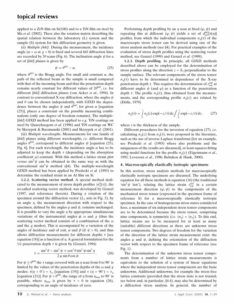
4.1.1. sin2w–sin(2w) method: analysis of a triaxial stressstate. The general strain–stress relation, equation (16), can be

rewritten as

"hkl’ ¼

12 Shkl

2 h�S’i ÿ h�

S33i

ÿ �sin2 þ h�S

’i sinð2 Þ� �

þ "hkl’0� ð28Þ

using the abbreviations h�S’i, h�

S’i and "hkl

’0� :

h�S’i ¼ h�

S11i cos2 ’þ h�S

12i sinð2’Þ þ h�S22i sin2 ’; ð29Þ

h�S’i ¼ h�

S13i cos’þ h�S

23i sin ’ ð30Þ

topical reviews


Figure 7Stress analysis employing the sin2 –sin (2 ) method: calculated example. Lattice strain for the 331 reflection of a macroscopically elastically isotropiccopper specimen subjected to the stress state given by the mechanical stress tensor in the figure: (a) at ’ = 0�, (b) at ’ = 45� and (c) at ’ = 90� (filled circlesfor positive tilt, open circles for negative tilt). The components of the stress tensor can be obtained on the basis of plots of aþ’ versus sin2 (d) and aÿ’versus sin (2 ) (e) (shown for ’ = 0�). For details, see text.

and

"hkl’0� ¼

12 Shkl

2 h�S33i þ Shkl

1 h�S11i þ h�

S22i þ h�

S33i

ÿ �: ð31Þ

For the determination of the off-diagonal stress tensor

components, a procedure suggested by Dolle & Hauk (1976)

can be employed (see also Evenschor & Hauk, 1975). An

example of a stress analysis on the basis of this method is

shown in Fig. 7.

For a general stress state, the lattice strain "hkl’ is neither a

linear function of sin2 nor a linear function of sin(2 ). The

parameters aþ’ and aÿ’ are obtained from the lattice strains

"hkl’ >0 and "hkl

’ <0 for a given ’, at fixed | |, i.e. by using lattice

strain measurements at positive and negative values of the

angle , respectively:

aþ’ ¼12 "

hkl’ >0 þ "

hkl’ <0

ÿ �¼ 1

2 Shkl2 h�

S’i ÿ h�

S33i

ÿ �sin2 þ "hkl

’0�

ð32Þ

and

aÿ’ ¼12 "

hkl’ >0 ÿ "

hkl’ <0

ÿ �¼ 1

2 Shkl2 h�

S’i sin 2 ð Þ: ð33Þ

Linear relations are now obtained for aþ’ (when plotted versus

sin2 ) and aÿ’ [when plotted versus sin(2 )]. Note that by

introducing aþ’ and aÿ’ , the shear components h�S13i and h�S

23i

are treated independently from the other components of the

stress tensor. The lattice strain is measured at three rotation

angles ’ = 0, 90 and 45� for several pairs of positive and

negative values of the angle . Then, a plot of the data for aþ’versus sin2 leads to a straight line (Fig. 7). The slope Aþ’ can

be written as [cf. equations (29) and (32)]:

Aþ’ ¼12 Shkl

2

"h�S

11i þ h�S22i

2þh�S

11i ÿ h�S22i

2cos 2’ð Þ

þ h�S12i sin 2 ’ð Þ ÿ h�S

33i

#: ð34Þ

The slopes at the specific ’ angles, Aþ0� , Aþ90� and Aþ45� , present

three equations for the four unknown stress components h�S11i,

h�S22i, h�

S33i and h�S

12i.

The component h�S12i can be directly calculated from

h�S12i ¼

112 Shkl

2

Aþ45� ÿAþ0� þ Aþ90�

2

� �: ð35Þ

For the other three unknown components, an additional

equation is needed, which is provided by equation (31). The

lattice strain "hkl’0� is measured at = 0� (it is advised to

determine an average of measurements at several ’ angles).

From equation (31) and from the quantities Aþ0� and Aþ90�

[equation (34)] it follows that

h�S33i ¼

112 Shkl

2 þ 3 Shkl1

"hkl’0� ÿ

Shkl1

12 Shkl

2

Aþ0� þ Aþ90�

ÿ �� ; ð36Þ

h�S11i ¼

Aþ0�12 Shkl

2

þ h�S33i ð37Þ

and

h�S22i ¼

Aþ90�

12 Shkl

2

þ h�S33i: ð38Þ

The shear stress components h�S13i and h�S

23i are derived from

h�S’i [equation (30)] as follows.

Plots of aÿ’ for ’ = 0 and 90� (Fig. 7) versus sin(2 ) lead to

straight lines (with offset = 0) with slopes Aÿ0� and Aÿ90� ,

respectively. The shear components h�S13i and h�S

23i are

obtained from

h�S13i ¼

Aÿ0�12 Shkl

2

ð39Þ

and

h�S23i ¼

Aÿ90�

12 Shkl

2

: ð40Þ

It should be mentioned that two situations occurring

frequently in practice, which can be handled by the above-

described method, are: (i) triaxial with h�S33i = 0, but h�S

i3i =

h�S3ii 6¼ 0 for i = 1, 2; note that in this case, knowledge of the

absolute strain at = 0�, "hkl’0� , is not required, cf. equation (36);

(ii) triaxial with h�S33i = 0, but h�S

i3i = h�S3ii 6¼ 0 for i = 1, 2 and

principal axes known with respect to the in-plane directions

(i.e. h�S12i = 0); note that in this case, knowledge of the absolute

strain at = 0�, "hkl’0� , is not required, cf. equation (36), and

measurements at ’ = 45� are not necessary, cf. equation (35).

The general method described above can be considerably

simplified when the number of non-zero stress tensor

components is reduced. The following simplifications with

respect to the general triaxial case (six unknown non-zero

stress tensor components) can be considered.

(i) Triaxial with principal axes known (three non-zero stress

tensor components).

(ii) Biaxial with principal axes unknown (three non-zero

stress tensor components).

(iii) Biaxial with principal axes known (two non-zero stress

tensor components).

(iv) Biaxial, rotationally symmetric (one independent non-

zero stress tensor component).

(v) Uniaxial (one independent non-zero stress tensor

component).

In the following, these methods are referred to as variants

of the sin2 method because in these cases, plots of lattice

strain versus sin2 suffice for stress analysis and no special

quantities as in the case of a triaxial stress state (like aþ’ ; see

above) have to be considered.

4.1.2. sin2w method: analysis of a triaxial principal stressstate. For a triaxial principal state of stress, the unknown stress

tensor components are h�S11i (=h�P

11i), h�S22i (=h�P

22i) and h�S33i

(=h�P33i). The strain–stress relation, equation (16), simplifies to

"hkl’ ¼

12 Shkl

2 cos2 ’h�S11i þ sin2 ’h�S

22i ÿ h�S33i

ÿ �sin2

þ Shkl1 h�

S11i þ h�

S22i þ h�

S33i

ÿ �þ 1

2 Shkl2 h�

S33i: ð41Þ

For ’ = 0�, equation (41) reads:

topical reviews


"hkl0� ¼

12 Shkl

2 h�S11i ÿ h�

S33i

ÿ �sin2

þ Shkl1 h�

S11i þ h�

S22i þ h�

S33i

ÿ �þ 1

2 Shkl2 h�

S33i: ð42Þ

For ’ = 90�:

"hkl90� ¼

12 Shkl

2 h�S22i ÿ h�

S33i

ÿ �sin2

þ Shkl1 h�

S11i þ h�

S22i þ h�

S33i

ÿ �þ 1

2 Shkl2 h�

S33i: ð43Þ

For = 0�:

"hkl’0� ¼ Shkl

1 h�S11i þ h�

S22i þ h�

S33i

ÿ �þ 1

2 Shkl2 h�

S33i: ð44Þ

The lattice strain is measured at two rotation angles ’ = 0 and

90� for a fixed hkl reflection at several tilt angles (cf. Hauk,

1997). The slopes, A0� and A90� , taken from the straight lines

obtained in plots of "hkl0� and "hkl

90� , respectively, versus sin2 [equations (42) and (43)] present two equations for the

stresses h�S11i, h�

S22i and h�S

33i. The third equation for the

determination of the three stress components is obtained from

"hkl’0� , i.e. a measurement at = 0�, equation (44) (where in

practice an average over measurements at several ’ angles is

recommended).

Solving the three equations for the three (principal) stress

components gives:

h�S33i ¼

112 Shkl

2 þ 3 Shkl1

"hkl’0� ÿ

Shkl1

12 Shkl

2

A0� þ A90�

ÿ �� ; ð45Þ

h�S11i ¼

A0�

12 Shkl

2

þ h�S33i ð46Þ

and

h�S22i ¼

A90�

12 Shkl

2

þ h�S33i: ð47Þ

4.1.3. sin2w method: analysis of a biaxial stress state. For a

plane state of stress, where the two principal axes are

unknown (but in the plane of the surface of the specimen), the

occurring stress components are h�S11i, h�

S22i and h�S

12i (stress

perpendicular to the surface, h�S33i, is zero) and thus equation

(16) becomes

"hkl’ ¼

12 Shkl

2 cos2 ’h�S11i þ sin 2 ’ð Þh�S

12i þ sin2 ’h�S22i

� �sin2

þ Shkl1 h�

S11i þ h�

S22i

ÿ �: ð48Þ


"hkl0� ¼

12 Shkl

2 h�S11i sin2 þ Shkl

1 h�S11i þ h�

S22i

ÿ �: ð49Þ

For ’ = 90�:

"S90� ¼

12 Shkl


1 h�S11i þ h�

S22i

ÿ �: ð50Þ

For ’ = 45�:

"S45� ¼

12 Shkl

2

h�S11i þ h�

S22i

2þ h�S

12i

� �sin2

þ Shkl1 h�

S11i þ h�

S22i

ÿ �: ð51Þ

The slopes deduced from the straight lines drawn through the

data in the three sin2 plots [according to equations (49)–

(51)] for ’ = 0, 45 and 90�, respectively, present a set of three

equations from which the three stress components h�S11i, h�

S22i

and h�S12i can be calculated in a straightforward manner

following equations (46) and (47) (with h�S33i = 0).

4.1.4. sin2w method: analysis of a biaxial principal stressstate. For a biaxial state of stress, i.e. non-zero and unequal

components h�S11i and h�S

22i (stress perpendicular to the

surface, h�S33i, is zero), the strain–stress relation, equation (16),

becomes

"hkl’ ¼

12 Shkl

2 cos2 ’h�S11i þ sin2 ’h�S

22iÿ �

sin2

þ Shkl1 h�

S11i þ h�

S22i

ÿ �: ð52Þ

In this case two series of measurements have to be performed

along the principal axes in the sample plane, i.e. at ’ = 0 and

90�.


"hkl0� ¼

12 Shkl


1 h�S11i þ h�

S22i

ÿ �: ð53Þ

For ’ = 90�:

"S90� ¼

12 Shkl


1 h�S11i þ h�

S22i

ÿ �: ð54Þ

The lattice strain is measured for several angles at ’ = 0 and

90�.

The two plots of "hkl0� and "hkl

90� , respectively, versus sin2 lead to straight lines and the (principal) stresses h�S

11i and h�S22i

are obtained from the slopes.

4.1.5. sin2w method: analysis of a rotationally symmetricbiaxial stress state. For a rotationally symmetric biaxial state

of stress the non-zero components of the stress tensor are h�S11i

= h�S22i = h�S

k i (stress perpendicular to the surface, h�S33i, is

zero) and the general strain–stress relation, equation (16),

reduces to (there is no ’ dependence):

"hkl ¼ 2 Shkl

1 þ12 Shkl

2 sin2 ÿ �

h�Sk i: ð55Þ

The strain "hkl is measured at several angles. When "hkl

is

plotted versus sin2 , a straight line is obtained and the stress

h�Sk i can be deduced from the slope.

4.1.6. sin2w method: analysis of a uniaxial stress state. For

a uniaxial state of stress, the only non-zero component of the

stress tensor is h�S11i and the general strain–stress relation,

equation (16), reduces to

"hkl’ ¼ Shkl

1 h�S11i þ

12 Shkl

2 sin2 h�S11i cos2 ’

ÿ �: ð56Þ

The strain "hkl’ is measured at several angles at ’ = 0�. When

"hkl’ is plotted versus sin2 , a straight line is obtained and the

stress h�S11i can be deduced from the slope.

The diffraction stress analyses discussed until now for the

triaxial case and the different simplifications employ at most

three different ’ angles; i.e. the angle is the predominant

angle for the variation of the strain measurement direction.

Two methods for stress analysis employing predominantly

variation of the measurement direction by ’ angle variation

are discussed next.

4.1.7. u integral method: analysis of a triaxial stress state.

The strain "hkl’ in equation (13), being a function of ’ with

period 2�, can be conceived as a Fourier series in ’ up to the

second order (Lode & Peiter, 1981; Wagner et al., 1983):

topical reviews


"hkl’ ¼

P2

n¼0

An ð Þ cos n’ð Þ þ Bn ð Þ sin n’ð Þ; ð57Þ

with Fourier coefficients2

A0 ð Þ ¼ "S11 þ "

S22

ÿ �sin2 þ 2 "S

33 cos2 ; ð58Þ

A1 ð Þ ¼ "S13 sin 2 ð Þ; ð59Þ

A2 ð Þ ¼12 "

S11 ÿ "

S22

ÿ �sin2 ; ð60Þ

B1 ð Þ ¼ "S23 sin 2 ð Þ ð61Þ

and

B2 ð Þ ¼ "S12 sin2 : ð62Þ

Hence, the Fourier coefficients An( ) and Bn( ) can be

calculated by Fourier inversion of equation (57) from the

strain values "hkl’ measured at a fixed angle in the interval ’

= 0–2�:

An ð Þ ¼1

�

R2�0

"hkl’ cos n’ð Þ d’ ð63Þ

and

Bn ð Þ ¼1

�

R2�0

"hkl’ sin n’ð Þ d’: ð64Þ

Employing equations (63) and (64) for at least two angles,

all of the six independent components "Sij of the strain tensor

can be calculated from equations (58) to (62). The entire

components h�Siji of the stress tensor are then obtained from

Hooke’s law [see also equation (9) with S1 and 12 S2 substituted

by Shkl1 and 1

2 Shkl2 ]:

h�Siji ¼

112 Shkl

2

"Sij þ

ÿShkl1

12 Shkl

2 þ 3 Shkl1

"S11 þ "

S22 þ "

S33

ÿ ��ij

� �: ð65Þ

The reliability of the results can be improved by measuring at

more than two values of . Then [instead of solving directly

equations (58) to (62)] a least-squares optimization procedure

has to be adopted for the determination of the components of

the strain tensor "Sij.

4.1.8. cos2u method: analysis of a biaxial stress state.

Substituting sin2’ by 1 ÿ cos2’ in equation (48), the simpli-

fication of equation (16) for the stress state considered

becomes

"hkl’ ¼

12 Shkl

2

�cos2 ’ h�S

11i ÿ h�S22i

ÿ �þ sin 2 ’ð Þh�S

12i

þ h�S22i�

sin2 þ Shkl1 h�

S11i þ h�

S22i

ÿ �: ð66Þ

For a fixed value of , values for the parameters cþ and cÿ , as

determined by the strains "hkl’>0 and "hkl

’<0 , with |’| constant,

i.e. measured at positive and negative values of the angle ’,

respectively, are obtained from (see Ballard et al., 1997)

cþ ¼12 "

hkl’>0 þ "

hkl’<0

ÿ �¼ 1

2 Shkl2 h�

S11i ÿ h�

S22i

ÿ �sin2 cos2 ’þ 1

2 Shkl2 h�

S22i sin2

þ Shkl1 h�

S11i þ h�

S22i

ÿ �ð67Þ

and

cÿ ¼12 "

hkl’>0 ÿ "

hkl’<0

ÿ �¼ 1

2 Shkl2 h�

S12i sin2 sin 2 ’ð Þ: ð68Þ

Note that with this representation, i.e. by cþ and cÿ , the shear

component h�S12i is treated independently of the other stress

tensor components.

For a fixed value of and for a given reflection hkl, lattice

strains are measured for several pairs of positive and negative

values of the angle ’ (i.e. with |’| constant). Then a plot of cþ versus cos2’ leads to a straight line (Fig. 8). The slope, Cþ , and

the intercept with the cþ axis, Iþ , provide two equations for

the stress components h�S11i and h�S

22i, which can be solved as

h�S22i ¼

1

2 Shkl1 þ

12 Shkl

2 sin2 Iþ ÿ

Cþ Shkl1

12 Shkl

2 sin2

� �ð69Þ

and

h�S11i ¼

Cþ 12 Shkl

2 sin2 þ h�S

22i: ð70Þ

The plot of cÿ versus sin(2’) leads to a straight line (with zero

offset). The stress h�S12i is deduced from the slope (Fig. 8).

In the case that the stress state is a principal biaxial stress

state, the plot of cÿ versus sin(2’) is superfluous as h�S12i is

equal to zero.

4.2. Multiple hkl reflections

By measuring lattice strain using different reflections hkl,

i.e. by measuring at different Bragg angles �hkl, the direction of

the lattice strain measurement can be varied without tilting the

specimen physically in the diffractometer [cf. x3, equation

(25)]. This is important (i) for the application of grazing-

incidence diffraction where the fixed (and small) angle of

incidence of the X-ray beam poses restrictions for the angle ,

and (ii) for large samples that can be mounted, but not tilted in

the diffractometer.

However, the following methods can also be used in cases

where specimen tilt is possible.

4.2.1. g(w, hkl) method: analysis of a biaxial stress state. In

an evaluation of the stress from lattice strain measurements

for different reflections hkl, the dependence of the strain "hkl

on hkl has to be dealt with, which requires a modification of

the sin2 plot. Equation (48) [i.e. the simplification of equa-

tion (16) for a biaxial stress state] can be reformulated by

introducing

g ; hklð Þ ¼

12 Shkl

2

Shkl1

sin2 : ð71Þ

Thus, for ’ = 0�:

"hkl0�

Shkl1

¼ g ; hklð Þh�S11i þ h�

S11i þ h�

S22i

ÿ �: ð72Þ

For ’ = 90�:

topical reviews


2 Note that the components of the strain tensor "Sij should be written as {"S

ij}hkl.

For the sake of simplicity, the curly brackets and the indication of thereflection are omitted.

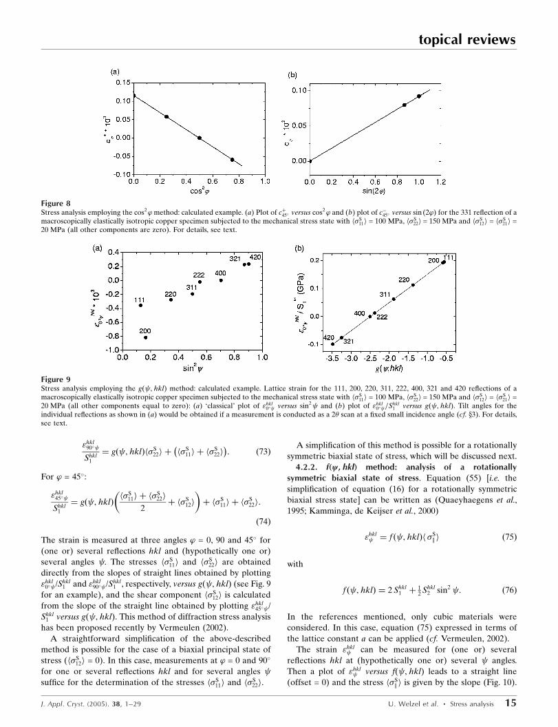
"hkl90�

Shkl1

¼ g ; hklð Þh�S22i þ h�

S11i þ h�

S22i

ÿ �: ð73Þ

For ’ = 45�:

"hkl45�

Shkl1

¼ g ; hklð Þh�S

11i þ h�S22i

2þ h�S

12i

� �þ h�S

11i þ h�S22i:

ð74Þ

The strain is measured at three angles ’ = 0, 90 and 45� for

(one or) several reflections hkl and (hypothetically one or)

several angles . The stresses h�S11i and h�S

22i are obtained

directly from the slopes of straight lines obtained by plotting

"hkl0� /Shkl

1 and "hkl90� /Shkl

1 , respectively, versus g( , hkl) (see Fig. 9

for an example), and the shear component h�S12i is calculated

from the slope of the straight line obtained by plotting "hkl45� /

Shkl1 versus g( , hkl). This method of diffraction stress analysis

has been proposed recently by Vermeulen (2002).

A straightforward simplification of the above-described

method is possible for the case of a biaxial principal state of

stress (h�S12i = 0). In this case, measurements at ’ = 0 and 90�

for one or several reflections hkl and for several angles suffice for the determination of the stresses h�S

11i and h�S22i.

A simplification of this method is possible for a rotationally

symmetric biaxial state of stress, which will be discussed next.

4.2.2. f(w, hkl) method: analysis of a rotationallysymmetric biaxial state of stress. Equation (55) [i.e. the

simplification of equation (16) for a rotationally symmetric

biaxial stress state] can be written as (Quaeyhaegens et al.,

1995; Kamminga, de Keijser et al., 2000)

"hkl ¼ f ; hklð Þh �S

k i ð75Þ

with

f ; hklð Þ ¼ 2 Shkl1 þ

12 Shkl

2 sin2 : ð76Þ

In the references mentioned, only cubic materials were

considered. In this case, equation (75) expressed in terms of

the lattice constant a can be applied (cf. Vermeulen, 2002).

The strain "hkl can be measured for (one or) several

reflections hkl at (hypothetically one or) several angles.

Then a plot of "hkl versus f( , hkl) leads to a straight line

(offset = 0) and the stress h�Sk i is given by the slope (Fig. 10).

topical reviews


Figure 8Stress analysis employing the cos2’method: calculated example. (a) Plot of cþ45� versus cos2’ and (b) plot of cÿ45� versus sin (2’) for the 331 reflection of amacroscopically elastically isotropic copper specimen subjected to the mechanical stress state with h�S

11i = 100 MPa, h�S22i = 150 MPa and h�S

12i = h�S21i =

20 MPa (all other components are zero). For details, see text.

Figure 9Stress analysis employing the g( , hkl) method: calculated example. Lattice strain for the 111, 200, 220, 311, 222, 400, 321 and 420 reflections of amacroscopically elastically isotropic copper specimen subjected to the mechanical stress state with h�S

11i = 100 MPa, h�S22i = 150 MPa and h�S

12i = h�S21i =

20 MPa (all other components equal to zero): (a) ‘classical’ plot of "hkl0� versus sin2 and (b) plot of "hkl

0� =Shkl1 versus g( , hkl). Tilt angles for the

individual reflections as shown in (a) would be obtained if a measurement is conducted as a 2� scan at a fixed small incidence angle (cf. x3). For details,see text.

4.3. General least-squares analysis of any stress state

All methods presented so far have in common that they

have been designed in such a way that stress tensor compo-

nents can be obtained on the basis of linear regressions. In

view of today’s computing power, the use of linear repre-

sentations is in principle not necessary for data evaluation.

Using non-linear least-squares fitting algorithms, which are

readily available (see, for example, Press et al., 1986), the

fitting of measured data for parameters obeying known

analytical expressions is straightforward. Thus, a powerful

alternative to the above-described methods is to determine

the unknown stress tensor components by least-squares

minimization of the difference �2 of the lattice strains calcu-

lated from equation (16), "calci ðh�

Si; hkl; ’; Þ, and the

measured lattice strains, "measi ðhkl; ’; Þ, where the unknown

mechanical stress tensor components h�Siji are the fit para-

meters:

�2 ¼P

i

!2i "

calci h�Si; hkl; ’; ÿ �

ÿ "measi hkl; ’; ð Þ

� �2: ð77Þ

The index i stands for all measured strains (for all different ,

’ and/or hkl used in the measurements) and the corresponding

calculated strains. The !i are weighing factors which can be

used to express the statistical relevance of the measured

strains "measi ðhkl; ’; Þ in the result of the minimization and

can be taken as the inverse of the standard deviations of the

measured strains. This is the most general solution method for

the determination of mechanical stress from measured lattice

strains (cf. x5.2). This approach was first employed by

Winholtz & Cohen (1988); see also Ortner (1986a,b). This

approach also allows a rigorous estimation of the statistical

errors of the stress tensor components to be determined, on

the basis of the given !i values [see equation (77); cf. Press et

al., 1986].

A major advantage of the approach is that the lattice strain

measurement directions ’ and and the number of reflections

used simultaneously can be chosen much more flexibly as

compared with the traditional methods. Whereas measure-

ments for a particular reflection at three angles of ’ are

needed in the traditional sin2 –sin(2 ) method for a full

stress tensor analysis, as an example, the general least-squares

analysis would allow at the same time the use of lattice strains

measured for different reflections. Thus, the analysis can be

completed when measured lattice strains are missing for a full

analysis using the sin2 –sin(2 ) method or the result can be

made more reliable by increasing the number of experimental

lattice strains used simultaneously. An example where five

unknown stress tensor components have been simultaneously

fitted to lattice spacing data measured at three different

rotation (’) angles is shown in Fig. 11.

Simplifications of the most general case (i.e. six unknown

stress tensor components have to be determined) can be

treated straightforwardly by not considering known stress

tensor components as fitting parameters but setting those

components as fixed. For example, in the case of a biaxial

rotationally symmetric stress state, only one fitting parameter

remains: the stress in the plane of the specimen h�Sk i = h�S

11i =

h�S22i, while the other stress tensor components can be set to

zero. An example of such an analysis is shown in Fig. 12.

An advantage of a linear-regression analysis (see xx4.1 and

4.2) is the simple visualization of the results of a stress analysis

in terms of linear plots such as sin2 plots. By eye, it can, for

example, be easily checked if a sin2 plot is linear or if the

number of measured data points and the range of tilt angles

used are sufficient. It is recommended to present the results of a

general non-linear least-squares analysis also in the form of

sin2 plots, because such plots will provide an additional

measure of the goodness-of-fit and/or the validity of the

underlying assumptions (such as macroscopic elastic isotropy

of the sample).

4.4. Comments

In this section some (brief) comments on the methods

described so far are given, which may be helpful for

performing a practical diffraction stress analysis.

4.4.1. Calculation of the lattice strain from the measuredlattice spacing. From a diffraction measurement, the spacing

topical reviews


Figure 10Stress analysis employing the f( , hkl) method: calculated example. Lattice strain for the 111, 200, 220, 311, 222, 400, 321 and 420 reflections of amacroscopically elastically isotropic copper specimen subjected to the mechanical stress state with h�S

11i = h�S22i = 100 MPa (all other components are

zero): (a) plot of "hkl versus sin2 and (b) plot of "hkl

versus f( , hkl). Tilt angles for the individual reflections as shown in (a) would be obtained if ameasurement is conducted as a 2� scan at a fixed small incidence angle (cf. x3). For details, see text.

of the {hkl} lattice planes can be directly obtained [equation

(2)], whereas the lattice strain has to be calculated from [cf.

equation (3)]

"hkl’ ¼

dhkl’ ÿ dhkl

0

dhkl0

ð78Þ

with dhkl0 as the strain-free lattice spacing of the {hkl} planes.

Equation (78) deserves some discussion with respect to

possible errors. From equation (78), it follows that

� "hkl’

ÿ �¼ ÿ cot �hkl

’

ÿ �� hkl

’

ÿ �ÿ� dhkl

0

ÿ �=dhkl

0 ; ð79Þ

topical reviews


Figure 11Stress analysis employing a general least-squares analysis: practical example. Lattice spacing for the 013 reflection of a macroscopically elasticallyisotropic Zircaloy specimen at three different rotation angles ’ (0, 45 and 90�) measured at positive (open circles) and negative (full circles) specimen tilt.Fitting was performed using five independent stress tensor components: h�S

11i, h�S22i, h�

S12i, h�

S13i, h�

S23i (h�S

33i was set to zero); the calculated lattice strainsare indicated by the lines in the figure. In addition, the strain-free lattice spacing for the {013} planes was used as a fit parameter in order to fit data on thebasis of lattice spacing instead of lattice strains. The results are indicated by the stress tensor in the figure. The error for the diagonal components is10 MPa; the error for the off-diagonal components is 2 MPa. The strain-free lattice spacing is used only as a dummy parameter. It could be used for thedetermination of the strain-free lattice constants only after correction for instrumental aberrations (cf. x4.4.1).

Figure 12Stress analysis employing a general least-squares analysis: practical example. Lattice spacing for the 111 (a) and 200 (b) reflections of a macroscopicallyelastically isotropic copper specimen (practically untextured thin film of thickness of about 0.5 mm, produced by physical vapour deposition). Fitting wasperformed using one independent stress tensor component: h�S

11i = h�S22i (all other components are zero). In addition, the strain-free lattice spacings for

the {111} and {200} planes were used as fit parameters in order to fit data on the basis of lattice spacing instead of lattice strains. The result is: h�S11i= h�

S22i

= 282 � 7 MPa. The strain-free lattice spacings are used only as dummy parameters. They could be used for the determination of the strain-free latticeconstants only after correction for instrumental aberrations (cf. x4.4.1).

i.e. errors (deviations) �ð"hkl’ Þ can be due to errors in the

measured peak positions or in the values used for the strain-

free lattice spacings.

A small error in the strain-free lattice spacing can cause a

relatively large error in the strain. As the strains in the elastic

regime are usually very small (<0.1%), the lattice spacings

have to be known with an accuracy better than of the order of

0.01%. In principle, strain-free lattice spacings can be deter-

mined by measuring a strain-free reference sample of the same

material as the sample under investigation. However, this can

be problematic in practice; for example, strain-free powders of

f.c.c. metals, prepared by filing and subsequent annealing,

usually contain stacking faults which give rise to shifts of the

measured Bragg angles. It is even impossible for materials

where the chemical composition or the amount of impurities is

not exactly known or for thin films consisting of a metastable

phase which cannot be produced as a strain-free bulk (or

powder) reference sample. In particular, the exploration of

stress gradients can be complicated in the presence of a

gradient of the strain-free lattice spacing, e.g. due to a non-

uniform chemical composition (see, for example, Somers &

Mittemeijer, 1990).

An apparent strain-free lattice spacing dhkl0 can be deter-

mined directly from the measurement of the strained sample.

It is given by the measured lattice spacing at those angles ’and for which, according to the theory, the strain is expected

to be zero. In the case of a rotationally symmetric biaxial state

of stress, for example, the direction, *, of zero strain is given

by sin2 * = ÿ2Shkl1 /ð12 Shkl

1 Þ [cf. equation (55)]. A detailed

discussion of the stress-free direction for more complicated

stress states and the relation with the stress component h�S33i

can be found in the textbook by Hauk (1997, x2.11 therein). In

the case of the presence of instrumental errors or imprecisely

known elastic constants, the thus determined apparent strain-

free lattice constant deviates from the true value. The elastic

constants are not required if lattice spacings are measured

under different load stresses. The strain-free direction, *, and

the strain-free lattice spacing, dhkl0 , are given by the intersec-

tion point of the dhkl’ versus sin2 plots for different load

stresses. For an investigation of invariant intersections in

diffraction stress analysis, see Hauk & Kruger (2000).

The error in the angular position, �hkl’ , of a diffraction line is

caused by instrumental aberrations. Peak shifts due to

instrumental aberrations can be, even for a well maintained

diffractometer, of the order of the peak shifts arising due to

the presence of stresses [for a detailed discussion on the effect

of instrumental errors in diffraction stress analysis, see, for

example, Noyan & Cohen (1987), Vermeulen (2000),

Vermeulen & Houtman (2000), and Leoni et al. (2004)]. Some

instrumental effects cause -independent errors of the peak

position (e.g. zero-offset of the 2� scale, cradle-axis misalign-

ment); i.e. peak shifts, but no absolute peak positions can be

reliably measured. Other instrumental effects cause -

dependent errors of the peak position (e.g. incident-beam

misalignment and specimen height displacement); i.e. neither

peak shifts nor absolute peak positions can be reliably

measured. It is useful to distinguish between errors leading to

�ð"hkl’ Þ independent of , in the following referred to as errors

of the first kind, and those leading to a �ð"hkl’ Þ depending on

, in the following referred to as errors of the second kind: the

different analysis methods, as discussed in this review, have

different susceptibilities to the two kinds of errors (see what

follows).

A constant error �ð"hkl’ Þ is only possible if the instrumental

error �ð�hkl’ Þ is constant (e.g. zero-offset of the 2� scale, cradle-

axis misalignment) and only one reflection [only one cotð�hkl’ Þ

in equation (79)] is used, or, in case of multiple hkl, if �ð�hkl’ Þ =

0 and �ðdhkl0 Þ/d

hkl0 = constant (independent of hkl). The error

in the strain-free lattice spacing, �ðdhkl0 Þ/d

hkl0 , is constant for

cubic systems (given by the error of the cell parameter),

whereas for all other crystal systems (involving several cell

parameters) it can depend on the reflection hkl.

Methods for the determination of the complete stress tensor;

methods involving more than one hkl reflection; cos2’ method.

These methods require the knowledge of absolute strains "hkl’

and the result of such an evaluation is susceptible to both

kinds of instrumental errors. As an example, it can be deduced

from equations (35)–(40) for the method of analysis described

in x4.1.1 (triaxial stress state), that only the determination of

the hydrostatic component �h = 13 ðh�

S11i + h�S

22i + h�S33iÞ of the

stress tensor requires the knowledge of absolute strains (and

thus of absolute peak positions), whereas the deviatoric

components are calculated employing only changes in strain

(and thus shifts of peaks).

If the presence of instrumental errors leading to an error of

the second kind �ð"hkl’ Þ cannot be excluded, it is generally

recommended to determine separately an (apparent) strain-

free lattice spacing, dhkl0;’ , for all ’, angles (and hkl reflec-

tions) involved in the analysis. This can be accomplished by

using a strain-free reference sample composed of the same

material as the sample under investigation (see, for example,

van Leeuwen et al., 1999). In this case, the lattice strain has to

be calculated from

"hkl’ ¼

dhkl’ ÿ dhkl

0;’

dhkl0;’

; ð80Þ

where the errors due to instrumental effects cancel out.

Alternative correction procedures involve analytical

expressions for the instrumental errors; see, for example,

Vermeulen & Houtman (2000) and Vermeulen (2000).

Methods for the determination of the stress tensor with

h�S33i = 0, involving only one hkl reflection. For the case that

h�S33i can be assumed to be zero, the methods employing only

one particular hkl reflection are susceptible to errors of the

second kind only (except the cos2’method; see above). These

methods do not require the knowledge of absolute strains:

relative strains suffice. The stress tensor components are not

influenced by an error of the first kind, because they are

determined from the slopes of plots of the strain versus (or

functions of ), such slopes not being affected by this kind of

error.

It should be noted that also in the general least-squares

fitting (x4.3), errors of the first kind �ð"hkl’ Þ play no role if

topical reviews


appropriate parameters, such as an apparent strain-free lattice

spacing, are included in the fit.

As a concluding remark, it is noted that an appropriate

choice of the diffractometer optics can substantially reduce

the significance of tilting-related instrumental errors. For

example, the use of parallel-beam optics may be preferred

over the use of focusing optics for precise stress measurements

(Leoni et al., 2004).

4.4.2. Miscellaneous. It is worth noting that the cos2’method (x4.1.8) is performed at a single angle . So absolute

values of the strains are needed for the determination of the

stresses (in contrast to the sin2 method, for example, where

the stress is determined from the slope of a plot of "hkl’ versus

sin2 ). If the actual stress-free lattice spacing of the sample is

different from the theoretical value, e.g. due to impurities,

errors in the stress values occur. For this reason, it is recom-

mended to determine experimentally the stress-free value

dhkl0;’ (see above).

With methods where X-ray elastic constants for at least two

reflections are involved in the calculation of a stress compo-

nent from a slope in a specific plot [f( , hkl) and g( , hkl)

methods], the criterion of linear behaviour of the considered

plot allows one to check if these XECs are consistent with the

investigated sample (see e.g. Vermeulen, 2002).

For cases where the principal axes of the state of stress are

unknown, an elliptical regression using various "hkl’ measure-

ments should be preferred rather than a linear regression in

order to determine shear stress components, as this method

handles the data more appropriately with respect to counting

statistics (cf. Fig. 11 for an experimental example).

4.4.3. Available methods for grazing-incidence diffraction.

For the case of grazing-incidence diffraction, the constraint of

a small and fixed incidence angle restricts the number of

applicable stress analysis methods (as described in x4 for

macroscopically isotropic materials) to the following cases.

(i) Wavelength fixed, variation of by use of multiple hkl:

f( , hkl) method (see x4.2.2) for a rotationally symmetric

biaxial state of stress, or g( , hkl) method (see x4.2.1) for a

biaxial state of stress.

(ii) hkl fixed, variation of by use of different wavelengths:

cos2’ method (x4.1.8) for a plane state of stress, or ’ integral

method (x4.1.7) for a triaxial state of stress.

5. Macroscopically elastically anisotropic specimens

5.1. Basis

Many specimens investigated by diffraction stress analysis

are not macroscopically elastically isotropic and, thus, the

methods of analysis described in x4 cannot, in principle, be

employed. Two sources of macroscopic elastic anisotropy can

be conceived: the occurrence of crystallographic texture (for

an overview, see, for example, Hauk, 1997) and the occurrence

of direction-dependent elastic grain interaction (van Leeuwen

et al., 1999; Welzel & Mittemeijer, 2003; Welzel et al., 2003;

Koch et al., 2004; Welzel, Leoni & Mittemeijer, 2004; for an

overview of various grain-interaction models, see Appendix

A).

For decades, only texture3 was considered as a possible

source of macroscopic elastic anisotropy, although the impact

of direction-dependent grain interaction on diffraction stress

analysis was discussed by Stickforth as long ago as 1966

(Stickforth, 1966), in particular in view of the occurrence of a

free surface for crystallites located within the surface region of

a polycrystalline aggregate. Direction-dependent grain inter-

action due to the occurrence of a free surface is called ‘surface

anisotropy’. Until recently, experimental investigations

yielded no evidence for the occurrence of ‘surface anisotropy’

in the stress analysis of surface regions of bulk materials by X-

ray diffraction (for an overview, see Hauk, 1997). Only

recently (van Leeuwen et al., 1999; Welzel et al., 2003), it was

demonstrated for the first time experimentally that, at least in

thin films, direction-dependent grain interaction can signifi-

cantly influence the dependence of lattice strain on the

direction of observation (see x5.2.2 and xA5.2; see, in parti-

cular, Welzel, Leoni & Mittemeijer, 2004). It was also shown

very recently that the occurrence of a grain-shape (morpho-

logical) texture results in direction-dependent grain interac-

tion and thus in macroscopic elastic anisotropy (Koch et al.,

2004).

In the case of a macroscopically elastically anisotropic

specimen, the so-called diffraction (X-ray) stress factors have

to be used for diffraction stress analysis [cf. equation (17) and

its discussion in x2; see also Welzel & Mittemeijer, 2003]:

f"L33g

hkl’ ¼ Fijð’; ; hklÞh�S

iji: ð81Þ

Whereas diffraction stress analysis for macroscopically elas-

tically isotropic (quasi-isotropic) specimens on the basis of

equation (16) has been extensively performed in the past, only

a very limited number of investigations have been dedicated

to macroscopically elastically anisotropic specimens. The

consequence of texture on diffraction stress analysis has not

generally been treated in review papers (cf. Table 1). This may

be owing to the complications caused by the occurrence of

macroscopic elastic anisotropy: the texture has to be described

quantitatively, i.e. either in terms of ideal orientations or in

terms of the orientation distribution function, and/or an

appropriate direction-dependent grain-interaction model is

required.

When the texture is very sharp and strong, it may be

described by single-crystal-like ideal orientations. The corre-

sponding diffraction stress analysis method is called the crys-

tallite group method (Willemse & Naughton, 1985; Willemse

et al., 1982; Hauk & Vaessen, 1985; Hauk, 1986; Hauk &

Oudelhoven, 1988; Baron & Hauk, 1988). In this limit, single-

crystal elastic compliances can be used and grain interaction

can be ignored, i.e. adoption of a grain-interaction model is

not necessary.

topical reviews


3 The notion texture without further specification refers to the occurrence ofcrystallographic, not morphological, texture in the following.

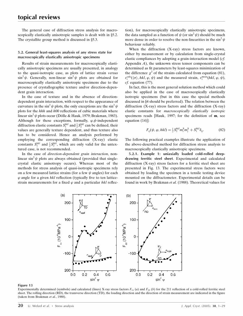
The general case of diffraction stress analysis for macro-

scopically elastically anisotropic samples is dealt with in x5.2.

The crystallite group method is discussed in x5.3.

5.2. General least-squares analysis of any stress state formacroscopically elastically anisotropic specimens

Results of strain measurements for macroscopically elasti-

cally anisotropic specimens are usually presented, in analogy

to the quasi-isotropic case, as plots of lattice strain versus

sin2 . Generally, non-linear sin2 plots are obtained for

macroscopically elastically anisotropic specimens due to the

presence of crystallographic texture and/or direction-depen-

dent grain interaction.

In the case of texture and in the absence of direction-

dependent grain interaction, with respect to the appearance of

curvature in the sin2 plots, the only exceptions are the sin2 plots for the hhh and h00 reflections of cubic materials where

linear sin2 plots occur (Dolle & Hauk, 1979; Brakman, 1983).

Although for these exceptions, formally, ’, -independent

diffraction elastic constants Shkl1 and 1

2 Shkl2 can be defined, their

values are generally texture dependent, and thus texture also

has to be considered. Hence an analysis performed by

employing the corresponding diffraction (X-ray) elastic

constants Shkl1 and 1

2 Shkl2 , which are only valid for the untex-

tured case, is not recommended.

In the case of direction-dependent grain interaction, non-

linear sin2 plots are always obtained (provided that single-

crystal elastic anisotropy occurs). Whereas most of the

methods for stress analysis of quasi-isotropic specimens rely

on a few measured lattice strains (for a few angles) for each

’ angle for a given hkl reflection (typically five to ten lattice-

strain measurements for a fixed ’ and a particular hkl reflec-

tion), for macroscopically elastically anisotropic specimens,

the data sampled as a function of (or sin2 ) should be much

more dense in order to resolve the non-linearities in the sin2 behaviour reliably.

When the diffraction (X-ray) stress factors are known,

either by measurement or by calculation from single-crystal

elastic compliances by adopting a grain-interaction model (cf.

Appendix A), the unknown stress tensor components can be

determined as fit parameters by least-squares minimization of

the difference �2 of the strains calculated from equation (81),

"calci ðh�i; hkl; ’; Þ and the measured strain, "meas

i ðhkl; ’; Þ,cf. equation (77).

In fact, this is the most general solution method which could

also be applied in the case of macroscopically elastically

isotropic specimens (but in this case the special methods

discussed in x4 should be preferred). The relation between the

diffraction (X-ray) stress factors and the diffraction (X-ray)

elastic constants for macroscopically elastically isotropic

specimens reads [Hauk, 1997; for the definition of m, see

equation (14)]:

Fijð ; ’; hklÞ ¼ 12 Shkl

2 mSi mS

j þ Shkl1 �ij: ð82Þ

The following practical examples illustrate the application of

the above-described method for diffraction stress analysis to

macroscopically elastically anisotropic specimens.

5.2.1. Example 1: uniaxially loaded cold-rolled deep-drawing ferritic steel sheet. Experimental and calculated

diffraction (X-ray) stress factors for a ferritic steel sheet are

presented in Fig. 13. The experimental stress factors were

obtained by loading the specimen in a tensile testing device

mounted on the diffractometer. Experimental details can be

found in work by Brakman et al. (1988). Theoretical values for

topical reviews


Figure 13Experimentally determined (symbols) and calculated (lines) X-ray stress factors F11 (a) and F22 (b) for the 211 reflection of a cold-rolled ferritic steelsheet. The rolling direction (RD), the transverse direction (TD), the loading direction and the direction of strain measurement are indicated in the figure(taken from Brakman et al., 1988).

the stress factors were calculated according to the Neerfeld–

Hill model, taking into account the texture information (a

rolling texture, in this case) in terms of the orientation

distribution function. From Fig. 13 it is evident that both the

experimentally determined and the calculated diffraction (X-

ray) stress factors exhibit distinct curvature; thus the experi-

mental sin2 dependence of the stress factors (i.e. of the

lattice strain) cannot be analysed at all on the basis of a

straight-line fit employing the sin2 formulation as for

macroscopically isotropic specimens [equation (16)].

By fitting the lattice strain calculated according to equation

(81) to the measured lattice strain as a function of sin2 by

minimizing �2 according to equation (77) using the stress

tensor components h�S11i and h�S

22i as fit parameters, the value

of the experimentally applied uniaxial load stress was

obtained from the diffraction stress measurement with very

good accuracy.

5.2.2. Example 2: textured thin copper layer exhibitinganisotropic elastic grain interaction. Two out of six " –sin2 diagrams as measured by X-ray diffraction are shown in Fig.

14 for a {111} fibre-textured copper film; the corresponding

calculated diagrams are also shown (200, 420 shown, 111, 220,

311, 331 not shown). For details of the deposition of the

copper layer and the diffraction measurement, together with a

detailed treatment of the diffraction stress analysis, see Welzel

et al. (2003). It was found experimentally that the measured

diffraction strain is independent of the sample rotation angle

’, and hence the stress state is rotationally symmetric (h�S11i =

h�S22i, h�

S12 ¼ 0i). Because the sample surface is unloaded, h�S

33i

= 0. Hence, only h�S11i = h�S

22i has to be determined by fitting

the lattice strain calculated according to equation (81) to the

measured lattice strain as a function of sin2 by minimizing �2

according to equation (77).

From Fig. 14 it is evident that the experimental sin2 dependence of the lattice strain cannot be analysed on the

basis of a straight-line fit employing the sin2 formulation as

for macroscopically isotropic specimens [equation (16)]. It

should be noted that all traditional grain-interaction models

(i.e. the Eshelby–Kroner model and any combination of the

Reuss grain-interaction model with the Voigt grain-interaction

model, e.g. the traditional Neerfeld–Hill model) predict linear

sin2 plots for the h00 (and hhh) reflection for textured

specimens composed of cubic crystallites; however, the

measured sin2 plot for the 200 reflection in Fig. 14 [and the

111 reflection, not shown in Fig. 14; see Welzel et al. (2003)]

cannot be described by a straight line. A so-called effective

direction-dependent grain-interaction model was developed

recently by Welzel et al. (2003). Only this direction-dependent

grain-interaction model, taking into account the effect of

elastic (surface) macroscopic anisotropy of the thin film, is

compatible with the curved behaviour in the sin2 plots

observed for the h00 (and the hhh, not shown) reflection. By

simultaneous fitting of the six measured sin2 plots, a very

satisfactory fit was achieved and a tensile in-plane stress of

165 MPa was determined (for details, see Welzel et al., 2003).

Note that for the calculation of the diffraction (X-ray) stress

factors, the (fibre-) texture of the specimen was fully taken

into account by using the experimentally determined (i.e.

calculated from measured pole figures) orientation distribu-

tion function.

5.3. Special method for textured macroscopically elasticallyanisotropic specimens: crystallite group method

A method for diffraction stress analysis of macroscopically

elastically anisotropic materials with strong and sharp texture

components (i.e. the orientation distribution function is

restricted to a number of localized maxima in Euler space) was

proposed by Willemse et al. (1982) and Willemse & Naughton

(1985). The method was adapted to rolled specimens by Hauk

& Vaessen (1985) (see also Hauk, 1986; Hauk & Oudelhoven,

1988; Welzel & Mittemeijer, 2004) and to fibre-textured

specimens by Baron & Hauk (1988). The concept of this

method will be revisited next.

In many practical cases, e.g. for cold-rolled materials, the

texture of a specimen may be described in terms of one or a

few so-called ideal orientations (crystallite groups), each

consisting of crystallites all with the same crystallographic

orientation (i.e. an ideal orientation is represented by a set of

crystallographically equivalent points in Euler space). Usually,

the Miller indices of the crystallographic planes oriented

parallel to the sample surface, {mnr}, and the indices of the S1

axis of the specimen frame of reference in the crystal frame of

reference, huvwi, are used for defining the orientation of a

particular crystallite group.

The strain tensor of a crystallite group in the specimen

frame of reference "S is related to the stress tensor �S by

Hooke’s law employing single-crystal elastic compliances

transformed to the specimen reference frame sSijkl:

"Sij ¼ sS

ijkl�Skl: ð83Þ

topical reviews


Figure 14Textured copper film. Measured (open circles) and simulated (dashedline) diffraction strain data for two reflections as function of sin2 (sin2 plots). For details of the simulation, see text. The error bars indicatingstatistical errors on the lattice strains are about twice the size of the circlesfor the 200 reflection and less than the size of the circles for the 420reflection.

In equation (83), "Sij and �S

kl have to be considered as averages

over all (spatially distributed) crystallites in the specimen

belonging to the crystallite group under consideration.

Equation (83) holds also for the lattice strain measured by

diffraction, provided that for the strain measurement, only

crystallites of the crystallite group under consideration

contribute to a diffraction line.

The measured lattice strain "’ can be calculated from the

strain tensor in the specimen frame of reference, "S, and the

unit vector, mS, in the direction of the diffraction vector as

expressed in the specimen frame of reference as follows:

"’ ¼ mSi mS

j "Sij ¼ mS

i mSj sS

ijkl�Skl: ð84Þ

As no distinction of diffraction strain and mechanical strain

has to be made for a crystallite group, the symbol "’ , i.e. the

strain in the direction of the (normalized) diffraction vector in

the specimen reference frame [cf. equation (14)] will be used

in the following.

By defining the transformation (rotation) matrix , trans-

forming from the (orthonormal) crystal frame of reference C

to the specimen frame of reference S, the compliance tensor

sSijkl can be expressed in terms of the compliance tensor in the

(orthonormal) crystal reference frame sCijkl, of which the

components are tabulated in various textbooks and databases:

sSijkl ¼ imjnkolpsC

mnop: ð85Þ

By insertion of equation (85) into equation (84), the strain can

be expressed as

"’ ¼ mSi mS

j imjnkolpsCmnop�

Skl; ð86Þ

which is the basic relation for diffraction stress analysis

according to the crystallite group method.

The measurement of the lattice strain of a crystallite group

using a particular hkl reflection is not possible for all combi-

nations of ’ and . As the diffraction vector has to be oriented

perpendicular to the {hkl} planes to obtain diffracted intensity,

an hkl reflection can only be found for certain combinations of

’ and , which are prescribed by the crystal structure of the

material and the orientation of the crystallite group under

investigation with respect to the specimen frame of reference.

On the one hand, this appears to be a limitation of the method

as the number of lattice strain measurements is limited to a

number of particular hkl reflections and orientations. On the

other hand, it is thus also possible to measure the lattice

strains for different crystallite groups in a specimen separately,

provided that enough hkl, ’ and combinations that are

unique for only one of the crystallite groups of the specimen

are indicated.

Because the components of the diffraction vector in the

specimen reference frame contain the factors sin and cos [cf. equation (14)], the orientation dependence of the lattice

strain is, as in the macroscopically elastically isotropic and

quasi-isotropic cases, dependent on the geometrical factors

sin cos = 12 sinð2 Þ and/or sin2 .

Two approaches to the stress determination by diffraction

on the basis of equation (86) are indicated.

Hauk & Vaessen (1985) (see also Hauk, 1986; Hauk &

Oudelhoven, 1988) used analytical simplifications of equation

(86) assuming: (i) a principal stress state (i.e. all off-diagonal

elements of the stress tensor expressed in the specimen

reference frame are zero) and (ii) cubic crystal symmetry. In

this case, the three unknown components (the principal

components) of the stress tensor can be determined from

measurements of the diffraction strain for ’ = 0 and 90� by

fitting of straight lines or elliptical curves using the stress

tensor components as fit parameters such that the strains

calculated from equation (86) match the measured strains, i.e.

by minimizing �2 defined by equation (77).

Ligot et al. (2004) suggested using equation (86) in a

numerical procedure such that computational evaluation

without analytical simplifications is possible. In this approach,

it is unnecessary to restrict the stress state to a principal stress

state or to limit the analysis to cubic crystal symmetry. Hence,

now six unknown tensor components can be obtained by

fitting the calculated strains using equation (86) to the

measured strains employing a least-squares minimization, i.e.

by minimizing �2 defined by equation (77). An additional

advantage of this approach is that the lattice strain measure-

ments need not be limited to certain specific orientations, as

given by ’ = 0 and 90�.

For polycrystalline specimens, the description of a (possibly

complex) texture in terms of a number of ideal orientations is

always a simplification: a continuous averaging of stress and

strain tensors in Euler space is replaced by a summation over

discrete ideal orientations only. For the stress tensor of the

specimen, for example, this simplification reads

h�i ¼R R

G

Rf gð Þ� gð Þ d3g ÿ!

CGMh�i ¼

P�

f�h��i; ð87Þ

where f� is the volume fraction of crystallites having a parti-

cular ideal orientation, thus forming the crystallite group �(greek symbols are used to avoid confusion with indices of

tensors, see equations below) and h��i is the average stress

tensor of this crystallite group.

In practice, also crystals exhibiting a (certain) small devia-

tion of their orientation from the ideal orientation are (have to

be) incorporated in the corresponding crystallite group.

Obviously, the approximation involved in replacing an

average in Euler space by a sum over discrete orientations is

the less severe the sharper the texture. However, not only the

non-ideality of the texture but also the type of grain interac-

tion acting in the specimen influences the severity of the

approximation involved in equation (87): only if the grain

interaction were of the Reuss type (all crystallites have the

same stress state) or if the specimen were to consist of only

one particular crystallite group, would equation (87) not be an

approximation. It has been demonstrated by Welzel &

Mittemeijer (2004) that additional errors can arise in the case

of non-ideal textures due to the impossibility to measure

lattice strains for individual crystallite groups separately.

Thus, it is generally not possible to estimate straightfor-

wardly the errors involved in employing equation (87) for

diffraction stress analysis.

topical reviews


5.3.1. Example. The following calculated example illustrates

the use of the crystallite group method in diffraction stress

analysis.

Mechanical (lattice) strains of the {211}h�1111i crystallite

group in a copper specimen, subjected to a biaxial stress state,

where h�S11i = 100 MPa and h�S

22i = 200 MPa, are presented in

Fig. 15 as a function of sin2 . The mechanical strain was

calculated using equation (86) (with single-crystal elastic

constants of copper) along three different directions, char-

acterized by the rotation angle ’ equal to 0, 74.77 and 90�,

respectively.

A measurement of the lattice (mechanical) strain of this

crystallite group is possible only for certain combinations of

the reflection (hkl) and the sample tilt ( ) and rotation (’)

angles. The strain data points which could be measured by

diffraction are marked by the symbols in Fig. 15. From these

lattice strains, if determined in a real measurement, the

(unknown) stress tensor components can be obtained on the

basis of equation (77) by fitting the calculated strains to the

measured strains [using equation (86) for the strain calcula-

tion].

Note that non-linear elliptic sin2 plots, as occur here, are

not necessarily an indication of the presence of shear stresses,

as would be the case for macroscopically isotropic specimens;

texture alone can cause this type of non-linearity (as is the

case here).

5.4. Concluding remarks

Both methods presented in x5 have their specific advantages

and limitations. The general analysis presented in x5.2 can be

applied to (in addition) all textured specimens. In addition to

the unknown stress tensor components, information about the

elastic grain interaction in the specimen can be obtained (cf.

x5.2.2). The analysis requires knowledge of the orientation

distribution function, calculation of diffraction stress factors

(cf. Appendix A) and non-linear least-squares fitting. The

crystallite group method presented in x5.3 should be consid-

ered as a simplification of the general method for (only)

specimens exhibiting a crystallographic texture, which,

furthermore, is both strong and sharp. This analysis is simple

and easily applicable: linear or elliptic curve fitting generally

suffices instead of non-linear least-squares fitting. The crys-

tallite group method requires a rather small number of lattice

strains measured at the intensity poles of the texture.

However, if the texture of the specimen is not sufficiently

sharp or consists of multiple components, application of this

method can give rise to significant errors, which cannot be

recognized without further ado.

Future research activities are required in particular for the

stress analysis of thin films and thin surface regions of bulk

polycrystals with respect to the occurrence of anisotropic grain

interaction. Origins of anisotropic grain interaction are

surface anisotropy and morphological (grain-shape) texture

(cf. Appendix A). Experimental investigation of diffraction

stress factors will be indispensable for the validation of grain-

interaction models.

APPENDIX AGrain-interaction models

Methods for diffraction stress analysis have been discussed in

xx4 and 5. For the practical application of any method, the

knowledge of diffraction (X-ray) elastic constants (for

macroscopically elastically isotropic specimens) or diffraction

(X-ray) stress factors (for macroscopically elastically aniso-

tropic specimens) is a prerequisite. Although a measurement

of diffraction (X-ray) elastic constants or diffraction (X-ray)

stress factors is possible by applying a known load stress to a

specimen under simultaneous lattice strain measurement in a

diffractometer, this approach is cumbersome and rarely used.

Generally, diffraction as well as macroscopic elastic constants

are calculated from single-crystal elastic constants by adopting

a grain-interaction model.

The basics common to all those grain-interaction models

considered are as follows (an exception is the Eshelby–Kroner

grain-interaction model and the reader is referred to xA3 for

details). For each crystallite, the stress and strain tensors in the

specimen reference frame are related by Hooke’s law:

"Sij ¼ sS

ijkl�Skl: ð88Þ

In equation (88), the sSijkl denote the single-crystal elastic

compliances expressed in the sample frame of reference.

Equation (88) represents a system of nine equations in eigh-

teen components, but as the strain and stress tensors are

symmetric (i.e. "ij = "ji and �ij = �ji), equation (88) is a short

notation for six independent equations with twelve indepen-

dent unknowns. If six components of the twelve unknowns are

known, the other six components can be calculated by solving

the system of equations (88). In the different types of grain-

interaction model considered here, a total of six stress and/or

topical reviews


Figure 15Illustration of the crystallite group method: calculated example. sin2 plots for the mechanical (lattice) strain for the crystallite group {211}h�1111iin a copper specimen subjected to a plane biaxial state of stress with �S

11 =100 MPa, �S

22 = 200 MPa for three values of ’ (lines). The symbolsindicate at which combinations of tilt ( ) and rotation (’) angles themeasurement of the lattice strain by diffraction is possible. As anexample, the lattice strain can be measured at sin2 = 0.25 and ’ = 90�,and at sin2 = 0.67 and ’ = 0� employing the 220 reflection.

strain tensor components in the specimen frame of reference

are taken to be equal to the mechanical averages for all

crystallites and thus the other six (unknown) components for a

crystallite can be calculated from the system of equations (88).

In the following, the commonly used grain-interaction

models are discussed and the basic equations necessary for

calculating diffraction (X-ray) elastic constants and diffraction

(X-ray) stress factors are given. For experimental investiga-

tions of diffraction elastic constants and validations of

different grain-interaction models, the reader is referred to e.g.

Brakman et al. (1988, Neerfeld–Hill model), Serruys et al.

(1987, 1989, Neerfeld–Hill model), Hauk & Nikolin (1989,

Eshelby–Kroner model), Behnken & Hauk (1991, Eshelby–

Kroner model) and Welzel et al. (2003, effective grain-inter-

action model for thin films).

A1. The Voigt model

The assumption for grain interaction in the Voigt model

(Voigt, 1910) is that the strain distribution is homogeneous in

the specimen, i.e. the strain tensor "S is the same for all crys-

tallites. This assumption implies that the aggregate remains

coherent when it is strained, since all crystallites are deformed

in exactly the same way. Thus, there is continuity of the strain

at the grain boundaries. As a consequence, the stress tensor is

different in each (differently oriented) crystallite. The

resulting discontinuities of the stress at the grain boundaries

violate mechanical equilibrium. As a consequence, this grain-

interaction model is generally not compatible with the

mechanical behaviour of real polycrystals. However, the Voigt

model is important in the context of effective grain-interaction

models (see xA5).

The X-ray stress factors can be calculated (see, for example,

Hauk, 1997) as follows:

Fijð ; ’; hklÞ

¼ mSk

R 2�

0 hcSðhkl; �; ’; Þiÿ1

ijkl f �ðhkl; �; ’; Þ d�R 2�

0 f �ðhkl; �; ’; Þ d�mS

l :

ð89Þ

In equation (89), cS denotes the single-crystal elastic stiffness

tensor expressed in the sample frame of reference. In the

absence of texture [f �ðhkl; �; ’; Þ � 1], the polycrystal is

macroscopically elastically isotropic, and thus the X-ray elastic


2 Shkl2 can be used instead of the stress

factors.

For cubic crystal symmetry, for example, the X-ray elastic

constants S1 and 12 S2 [cf. also equation (82) for the relation of

the X-ray stress factors to the X-ray elastic constants] can be

calculated from the components of the single-crystal compli-

ance tensor according to (Voigt, 1910; Reuss, 1929):

S1 ¼2 s0 s11 þ 2 s12ð Þ þ 5 s12 s44

6 s0 þ 5 s44

ð90Þ

and

12 S2 ¼

5 s11 ÿ s12ð Þs44

6 s0 þ 5 s44

ð91Þ

with

s0 ¼ s11 ÿ s12 ÿ s44=2: ð92Þ

Note that the XECs, according to the Voigt model, do not

depend on hkl and thus are equal to the mechanical constants.

A2. The Reuss model

The assumption for grain interaction in the Reuss model

(Reuss, 1929) is that the stress distribution is homogeneous in

the specimen, i.e. the stress tensor �S is equal for all crystal-

lites. As a consequence, the strain tensor is different in each

crystallite. This assumption implies that strain mismatch

occurs at grain boundaries. As a consequence, this grain-

interaction model is generally not compatible with the

mechanical behaviour of real polycrystals. However, the Reuss

model is important in the context of effective grain-interaction

models (see xA5).

The X-ray stress factors can be calculated (see, for example,

Hauk, 1997) as follows:

Fijð ; ’; hklÞ

¼ mSk

R 2�

0 sSðhkl; �; ’; Þijkl f �ðhkl; �; ’; Þ d�R 2�

0 f �ðhkl; �; ’; Þ d�mS

l :

ð93Þ

In the absence of texture [f �ðhkl; �; ’; Þ � 1], the polycrystal

is macroscopically elastically isotropic, and thus the X-ray

elastic constants Shkl1 and 1


factors.

For cubic crystal symmetry, for example, the X-ray elastic


2 Shkl2 can be calculated from the compo-

nents of the single-crystal compliance tensor according to

(Moller & Martin, 1939)

Shkl1 ¼ s12 þ s0 ÿ hklð Þ ð94Þ

and

12 Shkl

2 ¼ s11 ÿ s12 ÿ 3 s0 ÿ hklð Þ; ð95Þ

where ÿðhklÞ is the orientation factor for cubic materials:

ÿðhklÞ ¼ ðh2k2 þ h2l 2 þ k2l 2Þ= h2 þ k2 þ l 2ÿ �2

: ð96Þ

Note that the XECs according to the Reuss model are hkl

dependent.

A3. The Eshelby–Kroner model

In this model, the crystallites surrounding an individual

crystallite are conceived, in a statistical sense, as an elastically

homogenous matrix with the elastic properties of the entire

polycrystal. This model involves the solution of a so-called

inclusion problem (Eshelby, 1957), where the stress/strain

fields inside an inclusion embedded in a homogeneous matrix

have to be calculated on the basis of the underlying differ-

ential equations of the anisotropic elasticity theory. Rigorous

analytical solutions are only available for the case that the

topical reviews


matrix is elastically isotropic, the inclusion has a spherical

shape and the elastic properties of the inclusion exhibit cubic

symmetry (Kroner, 1958). The model was extended to the case

of crystallographically textured specimens by Kneer (1965).

The calculation in this case involves a spherical anisotropic

inclusion embedded in an elastically anisotropic matrix and

analytical solutions are no longer feasible. Instead, an iterative

numerical procedure has to be employed.

The basics are as follows. The elastic strain of a single-

crystalline inclusion (grain) in a polycrystalline aggregate can

be expressed as

"ij �; �; ð Þ ¼ Sijkl þ tijkl �; �; ð Þ� �

h�kli: ð97Þ

Obviously, the tensor t accounts for the deviation of the elastic

properties of an individual grain from the (average) elastic

properties of the entire polycrystal/surrounding matrix [cf.

equation (88)]. In this view, th�i is a strain in the individual

crystallite induced by the mismatch of the elastic constants of

a crystallite with respect to those of the matrix to be added to

the matrix-average strain contribution Sh�i to arrive at the

total strain " of the crystallite. The tensor t depends on the

shape of the inclusion, the single-crystal elastic constants and

the macroscopic mechanical compliance tensor S of the

aggregate. Usually, spherical inclusions are considered; this is

a valid assumption for the case of polycrystals consisting of

(on the average) equi-axed grains. For the case of a morpho-

logical (grain-shape) texture, e.g. ellipsoidal inclusions, all with

the same shape orientation, see Koch et al. (2004). Note that,

considering a morphological (grain-shape) texture, the

Eshelby–Kroner model becomes a direction-dependent grain-

interaction model, i.e. the grain-interaction assumptions along

different directions in the specimen are inequivalent; for

details, see Welzel, Freour & Mittemeijer (2004).

Averaging equation (97) over the entire specimen results in

h"iji ¼ Sijklh�kli ¼ hSijkl þ tijkl �; �; ð Þih�kli ð98Þ

and thus it must hold that

hti ¼ 0: ð99Þ

Generally, the components of the mechanical compliance

tensor S are, based on starting values, varied in an iteration

procedure until t satisfies the boundary condition expressed by

equation (99). Then, the X-ray stress factors can be calculated

from the thus determined values for S (see, for example, Hauk,

1997) as follows:

Fijð ; ’; hklÞ ¼mSk

n R2�0

�SSðhkl; �; ’; Þijkl þ tSðhkl; �; ’; Þijkl

�� f �ðhkl; �; ’; Þ d�

. R2�0

f �ðhkl; �; ’; Þ d�o

�mSl : ð100Þ

In the absence of crystallographic [f �ðhkl; �; ’; Þ � 1] and

morphological (grain-shape) texture, the polycrystal is

macroscopically elastically isotropic, and thus the X-ray elastic



factors.

For a crystallographically and morphologically untextured

(i.e. macroscopically elastically isotropic) specimen composed

of cubic crystallites, the XECs can be calculated from

(Bollenrath et al., 1967)4

S1 hklð Þ ¼ S12 þ T12 þ T0 ÿ hklð Þ ð101Þ

and

12 S2 hklð Þ ¼ S11 ÿ S12 þ T11 ÿ T12 ÿ 3 T0 ÿ hklð Þ ð102Þ

with

T0 ¼ T11 ÿ T12 ÿ 2T44 ð103Þ

and

ÿ hklð Þ ¼ ðh2k2 þ k2l2 þ l2h2Þ= h2 þ k2 þ l2ÿ �2

: ð104Þ

T11 and T12 can be calculated from

T11 ÿ T12 ¼Gÿ �ð Þ 3K þ 6Gð Þ

G 8G2 þG 9K þ 12�ð Þ þ 6�K½ �ð105Þ

and

2T44 ¼Gÿ �ð Þ 3K þ 6Gð Þ

G 8G2 þG 9K þ 12�ð Þ þ 6�K½ �ð106Þ

with

3K ¼ 1=ðS11 þ 2S12Þ; ð107Þ

where K is the bulk modulus,

� ¼ 1=S44 ð108Þ

and

2� ¼ 1=ðS11 ÿ S12Þ: ð109Þ

The shear modulus G can be obtained as the solution of the

following equation:

G3þ �G2

þ �Gþ ¼ 0; ð110Þ

where the following abbreviations have been used:

� ¼ ð9K þ 4�Þ=8; ð111Þ

� ¼ ÿ 3K þ 12�ð Þ�=8 ð112Þ

and

¼ ÿ3K��=4: ð113Þ

A4. The Vook–Witt and inverse Vook–Witt models

In a bulk specimen, each crystallite is surrounded by other

crystallites in three dimensions. In films, which often have a

columnar grain structure, each surface-adjacent crystallite is

surrounded by other crystallites in only two dimensions.

Owing to their microstructure and reduced dimensionality,

thin films cannot generally be considered as macroscopically

elastically isotropic. Rather they can exhibit macroscopically

transversely isotropic properties [even in the absence of

topical reviews


4 Note that the symbols �, �, , � and � bear no relation to the same symbolsused in earlier sections. These symbols are used here for consistency with thecited literature.

crystallographic texture (van Leeuwen et al. 1999)]. The

traditional models for grain interaction [Voigt, Reuss,

Eshelby–Kroner (involving spherical inclusions; cf. xA3),

Neerfeld–Hill] are compatible only with macroscopically

isotropic elastic properties (in the absence of crystallographic

texture) and are thus inappropriate for the analysis of stress in

thin films.

In the bulk of a polycrystal, with respect to grain interac-

tion, generally all (principal) directions are equivalent. For

this reason, the number of grain-interaction models of

extreme types of grain-interaction assumptions is two for bulk

materials (Reuss and Voigt, provided that all directions within

the bulk are equivalent for grain interaction). Columnar thin

films possess two principal directions exhibiting possibly

different types of grain interactions: the in-plane direction (all

in-plane directions are equivalent) and the direction perpen-

dicular to the surface of the film. On the basis of the same

reasoning, four types of extreme grain-interaction models can

then be formulated for columnar thin films, as two principal

directions, each with two possible extreme grain interactions,

occur. The Voigt and Reuss models have already been

discussed (xxA1 and A2). The two additional extreme grain-

interaction models are the Vook–Witt and inverse Vook–Witt

models. Such models, adopting different grain-interaction

assumptions along different (principal) directions in the

specimen, are called direction-dependent grain-interaction

models.

A4.1. The Vook–Witt model. Vook & Witt (1965) have

proposed a set of grain-interaction assumptions which reflect

transverse isotropy and thus may be applicable to thin films

[see van Leeuwen et al. (1999) for the case of untextured

specimens, and Leoni et al. (2001) for the case of (fibre-)

textured specimens]. An (at least) macroscopically elastically

transversely isotropic specimen subjected to a planar rota-

tionally symmetric state of stress is considered [for a gener-

alization to any stress state, see Welzel & Freour (2004)]. The

grain-interaction assumptions of the Vook–Witt model are

then: (i) the strain is rotationally symmetric in the plane of the

film and (ii) equal for all crystallites (Voigt-type grain inter-

action), and (iii) the stresses perpendicular to the layer are

zero for all crystallites (Reuss-type grain interaction), i.e. the

crystallites can deform freely in this direction. These

assumptions fix parts of the stress and strain tensor for all

crystallites:

"S¼

"Sk 0 �

0 "Sk �

� � �

0@ 1A ð114Þ

and

�S ¼

� � 0

� � 0

0 0 0

0@ 1A: ð115Þ

The tensor components marked by � are not explicitly speci-

fied for every crystallite, but these components can be calcu-

lated from Hooke’s law for every crystallite according to

equation (88). Thus, for a particular value of the strain parallel

to the substrate "Sk, all non-zero strain and stress tensor

components can be calculated by solving the system of

equations (88) (for explicit equations, see Leoni et al., 2001).

The Vook–Witt grain-interaction model may be more

appropriate for the analysis of macroscopic stress in thin films

than traditional grain-interaction models (such as the Reuss or

Voigt models). A remarkable feature of this grain-interaction

model is that, even in the absence of crystallographic texture,

the sin2 plots are non-linear (van Leeuwen et al., 1999; see

also x5.2.1).

A4.2. The inverse Vook–Witt model. The inverse Vook–

Witt model completes the set of four extreme grain-interac-

tion models for (columnar) thin films. As for the Vook–Witt

model, a transversely isotropic specimen subjected to a planar

rotationally symmetric state of stress is considered [for a

generalization to any stress state, see Welzel & Freour (2004)].

The grain-interaction assumptions are as follows: (i) the in-

plane stress is rotationally symmetric and (ii) equal for all

crystallites (Reuss-type grain interaction), and (iii) the strain

perpendicular to the film surface is equal for all crystallites

(Voigt-type grain interaction). Like in the (regular) Vook–

Witt model, these assumptions fix certain strain and stress

tensor components for all crystallites [cf. equations (114) and

(115)]:

"S¼

� � 0

� � 0

0 0 "S?

0@ 1A ð116Þ

and

�S ¼

�Sk 0 �

0 �Sk �

� � �

0@ 1A: ð117Þ

The missing strain and stress tensor components for each

crystallite, marked by �, can be calculated by solving the

system of equations (88).

The inverse Vook–Witt grain-interaction model is required

for the construction of an effective grain-interaction model for

thin films (see xA5). A remarkable feature of this grain-

interaction model is that, as for the Vook–Witt model, even in

the absence of crystallographic texture, the sin2 plots are non-

linear (Welzel et al., 2003).

A5. Effective grain-interaction models

The mechanical elastic constants, the X-ray elastic constants

and the X-ray stress factors calculated employing extreme

grain-interaction models are generally not compatible with the

real elastic behaviour of polycrystals. However, it often found

empirically that averaging the elastic constants of extreme

grain-interaction models results in elastic data that are

compatible with experimentally determined values. The

background of any averaging of (extreme) grain-interaction

models to represent physical reality could be described as

follows. A real sample is conceived to be constituted by

separate volume fractions of crystallites, each of which obeys a

certain type of grain interaction. For the following discussion,

topical reviews


an average of (extreme) grain-interaction models will be

called an effective grain-interaction model. Depending on the

type of specimen considered, appropriate choices of the grain-

interaction models ‘to be averaged’ can be made.

Under the assumption that a volume fraction fi of the

polycrystalline aggregate obeys the (extreme) grain-interac-

tion model i, average elastic constants can be calculated as an

arithmetic average:

� ¼P

i

fi�i; ð118Þ

where � stands for a certain elastic constant (e.g. Young’s

modulus or an X-ray elastic constant) andPi

fi ¼ 1: ð119Þ

A5.1. The Neerfeld–Hill model. The Voigt and Reuss

models are the extreme cases of grain interaction in bulk

polycrystals: either the strain tensor (Voigt model) or the

stress tensor (Reuss model) for each crystallite is assumed to

be equal to the mechanical strain or stress tensor, respectively;

they are therefore incompatible with physical reality because

of the corresponding stress, respectively strain discontinuities

at the grain boundaries. It was shown that the Voigt and Reuss

models set bounds for the mechanical elastic constants (Hill,

1952). Further, Neerfeld (1942) and Hill (1952), on an

empirical basis, suggested that the arithmetic (or geometric5;

Hill, 1952) average of X-ray (Neerfeld, 1942) and macroscopic

(Neerfeld, 1942; Hill, 1952) elastic constants calculated

according to the models of Voigt and Reuss, respectively, are

in better agreement with experimental data. This approach is

referred to as the Neerfeld–Hill model.

Generally, an arithmetic average where the Voigt and Reuss

contributions are both 1/2 is adopted (however, other

weighing schemes for the two extreme models could be

conceived):

�NH ¼ f �R þ 1ÿ fð Þ�V ð120Þ

where � stands for a certain elastic constant (e.g. Young’s

modulus or an X-ray elastic constant), the subscripts indicate

the grain-interaction models and f is a mixing parameter

(corresponding to the volume fraction of crystallites obeying

the Reuss model). This parameter may be used as an addi-

tional fit parameter in a general least-squares analysis (cf. xx4.3

and 5.2; see also Serruys et al., 1987, 1989).

A5.2. An effective grain-interaction model for thin films.Even though the Vook–Witt and inverse Vook–Witt grain-

interaction models can be considered as ‘intermediate’ models

of grain interaction (with reference to the extreme Voigt and

Reuss models), these models still involve extreme grain-

interaction assumptions along the two considered principal

directions.

An effective grain-interaction model for a thin film or,

possibly, for surface-adjacent material can be constructed

(Welzel et al., 2003). Consider the following example. The

Reuss model can be combined with the Vook–Witt model by

assuming that the specimen is composed of an effective

volume fraction fR of the sample obeying the Reuss model and

an effective volume fraction fVW obeying the Vook–Witt

model. Such a combined model leads, effectively, to partial in-

plane Reuss behaviour: whereas the crystallites are tightly

connected together with respect to the in-plane direction in

the Vook–Witt approach and exhibit identical strains, the

combination with the Reuss constraint gives the crystallites

some degree of freedom for in-plane deformation indepen-

dent of the neighbouring crystallites, thereby lifting the

(unrealistic) constraint of identical planar strain for every

crystallite. A similar discussion can be given for combinations

of other extreme grain-interaction models.

A quantification of the effect of model mixing on the grain

interaction can be achieved by defining interaction parameters

for the two principal directions.

(i) In-plane interaction parameter wk: equals one for a

Voigt-type interaction (crystallites are tightly connected

together) and zero for a Reuss-type interaction (crystallites

can deform independently of neighbouring crystallites, but

their stresses are identical).

(ii) The out-of-plane interaction parameter w?: definition

analogous to the in-plane parameter wk, i.e. w? equals one for

Voigt-type interaction and zero for a Reuss-type interaction.

Combining the models for extreme types of grain interac-

tion, results in average values hwki and hw?i for the interac-

tion parameters:

hwki ¼P

i

fiwk;i ð121Þ

and

hw?i ¼P

i

fiw?;i: ð122Þ

In equations (121) and (122), the fi represent, as in equation

(118), effective volume fractions of grains obeying the grain-

interaction model i. For a given combination of grain-inter-

action models, the average interaction parameters can be

calculated following equations (121) and (122).

Generally, the parameters fi are not known a priori. In this

case, the parameters fi may be used as additional fit para-

meters in a general least-squares analysis (cf. xx4.3 and 5.2; see

also Welzel et al., 2003).

References

Acker, K. van, de Buyser, L., Celis, J. P. & van Houtte, P. (1994). J.Appl. Cryst. 27, 56–66.

Ballard, B. L., Predecki, P. K., Watkins, T. R., Kozaczek, K. J., Braski,D. N. & Hubbard, C. R. (1997). Adv. X-ray Anal. 39, 363–370.

Baron, H. U. & Hauk, V. (1988). Z. Metallkd. 79, 41–49, 127–131.Behnken, H. & Hauk, V. (1991). Z. Metallkd. 82, 151–158.Behnken, H. & Hauk, V. (2000). In Proceedings of ICRS6, 10–12 July

2000, Oxford, pp. 277–282. London: IOM Communications.Bollenrath, F., Hauk, V. & Muller, E. H. (1967). Z. Metallkd. 58, 76–

82.

topical reviews


5 Usually the arithmetic and not the geometric average is used. Thegeometrical average of n numbers is defined as the nth root of the productof the numbers. For Young’s modulus, as an example, the geometric average ofthe moduli according to the Reuss (ER) and Voigt (EV) models EGA is definedas (EREV)1/2.

Bollenrath, F., Osswald, E., Moller, H. & Neerfeld, H. (1941). Arch.Eisenhuttenwesen, 15, 183–194.

Brakman, C. M. (1983). J. Appl. Cryst. 16, 325–340.Brakman, C. M., de Keiijser, Th. H., van der Pers, N. M., Penning, P. &

Radelaar, S. (1988). Philos. Mag. A, 58, 635–60.Bunge, H.-J. (1982). Texture Analysis in Materials Science. London:

Butterworths.Christenson, A. L. & Rowland, E. S. (1953). Trans. ASM, 45, 638–676.Delhez, R., de Keijser, Th. H. & Mittemeijer, E. J. (1982). Fresen. Z.

Anal. Chem. 312, 1–16.Delhez, R., de Keijser, Th. H. & Mittemeijer, E. J. (1987). Surf. Eng.

3, 331–342.Dolle, H. (1979). J. Appl. Cryst. 12, 489–501.Dolle, H. & Hauk, V. (1976). Hart.-Tech. Mitt. 31, 165–168.Dolle, H. & Hauk, V. (1978). Z. Metallkd. 69, 410–417.Dolle, H. & Hauk, V. (1979). Z. Metallkd. 70, 682–685.Dummer, T., Eigenmann, B., Stußer, M., Leiste, H., Lohe, D., Muller,

H. & Vohringer, O. (1999). Z. Metallkd. 90, 780–787.Eigenmann, B. & Macherauch, E. (1995). Mater.-Wiss. u. Werk-

stofftech. 26, 148–160, 199–216.Eigenmann, B. & Macherauch, E. (1996). Mater.-Wiss. u. Werk-

stofftech. 27, 426–437, 491–501.Eigenmann, B., Scholtes, B. & Macherauch, E. (1992). Residual

Stresses III, edited by H. Fujiwara, T. Abe & K. Tanaka, pp. 601–606. Amsterdam: Elsevier Applied Science.

Eshelby, J. D. (1957). Proc. R. Soc. A, 241, 376–396.Evenschor, P. D. & Hauk, V. (1975). Z. Metallkd. 66, 167–168.Giacovazzo, C., Monaco, H. L., Voterbo, D., Scordari, F., Gilli, G.,

Zanotti, G. & Catti, M. (1998). Fundamentals of Crystallography.Oxford: Oxford Science.

Genzel, Ch. (1994). Phys. Status Solidi A, 146, 629–637.Genzel, Ch. (1997). Phys. Status Solidi A, 159, 283–296.Genzel, Ch. (1999). J. Appl. Cryst. 32, 770–778.Genzel, Ch., Broda, M., Dantz, D. & Reimers, W. (1999). J. Appl.

Cryst. 32, 779–787.Hauk, V. (1952). Arch. Eisenhuttenwesen, 23, 353–361.Hauk, V. (1986). Adv. X-ray Anal. 29, 1–15.Hauk, V. (1995). Hart.-Tech. Mitt. 50, 138–144.Hauk, V. (1997). Editor. Structural and Residual Stress Analysis by

Nondestructive Methods. Amsterdam: Elsevier.Hauk, V. & Kruger, B. (2000). Mater. Sci. Eng. A, 284, 261–267.Hauk, V & Nikolin, H.-J. (1989). Z. Metallkd. 80, 862–872.Hauk, V. & Oudelhoven, R. (1988). Z. Metallkd. 79, 41–49.Hauk, V. & Vaessen, G. (1985). Z. Metallkd. 76, 102–107.Hill, R. (1952). Proc. Phys. Soc. London, 65, 349–354.Hoffman, R. W. (1966). The Mechanical Properties of Thin

Condensed Films, in Physics of Thin Films, Vol. 3, edited by G.Hass & R. E. Thun, pp. 211–273. New York: AcademicPress.

Hoffman, R. W. (1976). Mechanical Properties of Non-Metallic ThinFilms, in Physics of Non-Metallic Thin Films, edited by C. H. S.Dupuy & A. Cachard, Proceedings NATO Advanced StudyInstitutes Series, Series B: Physics, Vol. 14, pp. 273–353. New York:Plenum Press.

Kamminga, J. D., Delhez, R., de Keijser, Th. H. & Mittemeijer, E. J.(2000a). J. Appl. Cryst. 33, 108–111.

Kamminga, J. D., de Keijser, Th. H., Delhez, R. & Mittemeijer, E. J.(2000b). J. Appl. Cryst. 33, 1059–1066..

Kneer, G. (1965). Phys. Status Solidi, 9, 825–834.Koch, N., Welzel, U., Wern, H. & Mittemeijer, E. J. (2004). Philos.

Mag. 84, 3547–3570.Kroner, E. (1958). Z. Physik, 151, 504–518.Leeuwen, M. van, Kamminga, J.-D. & Mittemeijer, E. J. (1999). J.

Appl. Phys. 86, 1904–1914.Leoni, M., Welzel, U., Lamparter, P., Mittemeijer, E. J. & Kamminga,

J.-D. (2001). Philos. Mag. A, 81, 597–623.Leoni, M., Welzel, U. & Scardi, P. (2004). J. Res. Natl Inst. Stand.

Technol. 109, 27–48.

Leverenz, T., Eigenmann, B. & Macherauch, E. (1996). Z. Metallkd.87, 616–625.

Ligot, J., Welzel, U., Lamparter, P. & Mittemeijer, E. J. (2004). Inpreparation.

Lode, W. & Peiter, A. (1981). Metall, 35, 758–762.Ma, C.-H., Huang, J.-H. & Chen, H. (2002). Thin Solid Films, 418, 73–

78.Macherauch, E. & Muller, P. (1961). Z. Angew. Phys. 13, 305–312.Macherauch, E., Wohlfahrt, H. & Wolfstieg, U. (1973). Hart.-Tech.

Mitt. 28, 201.Machlin, E. S. (1995). Materials Science in Microelectronics, Vol. 2.

New York: Giro Press.Marra, W. C., Eisenberger, P. & Cho, A. Y. (1979). J. Appl. Phys. 50,

6927–6933.Meyers, M. A. & Chawla, K. K. (1984). Mechanical Metallurgy,

Principles and Applications. Englewood Cliffs, New Jersey:Prentice-Hall.

Mittemeijer, E. J. & Scardi, P. (2004). Editors. Diffraction Analysis ofthe Microstructure of Materials. Berlin: Springer.

Moller, H. & Barbers, J. (1935). Mitt. K.-Wilh.-Inst. Eisenforschg. 17,157–177.

Moller, H. & Martin, G. (1939). Mitt. K.-Wilh.-Inst. Eisenforschg. 21,261–269.

Neerfeld, H. (1942). Mitt. K.-Wilh.-Inst. Eisenforschg. 24, 61–70.Noyan, I. C. & Cohen, J. B. (1987). Residual Stress. Measurement by

Diffraction and Interpretation. New York: Springer.Noyan, I. C., Huang, T. C. & York, B. R. (1995). Crit. Rev. Solid State

Mater. Sci. 20, 125–177.Nye, J. F. (1957). Physical Properties of Crystals. Oxford University

Press.Ortner, B. (1986a). Adv. X-ray Anal. 29, 113–118.Ortner, B. (1986b). Adv. X-ray Anal. 29, 387–394.Parrat, L. G. (1954). Phys. Rev. 95, 359–369.Predecki, P., Ballard, B. & Zhu, X. (1993). Adv. X-ray Anal. 36, 237–

245.Press, W. H., Flannery, B. P., Teukolsky, S. A. & Vetterling, W. T.

(1986). Numerical Recipes. Cambridge University Press.Quaeyhaegens, C., Knuyt, G. & Stals, L. M. (1995). Surf. Coat.

Technol. 74–75, 104–109.Quaeyhaegens, C., Knuyt, G. & Stals, L. M. (1996). J. Vac. Sci.

Technol. A, 14, 2462–2468.Reuss, A. (1929). Z. Angew. Math. Mech. 9, 49–58.Roe, R.-J. & Krigbaum, W. R. (1964). J. Chem. Phys. 40, 2608–2615.Serruys, W., Van Houtte, P. & Aernoudt, E. (1987). In Residual

Stresses in Science and Technology, edited by E. Macherauch & V.Hauk, pp. 417–424. Oberursel: Deutsche Gesellschaft furMetallkunde.

Serruys, W., Langouche, F., van Houtte, P. & Aernoudt, E. (1989). InProceedings of ICRS2, edited by G. Beck, A. Denis & A. Simon, pp.166–171. London: Elsevier Applied Science.

Skrzypek, S. J. & Baczmanski, A. (2001). Adv. X-ray Anal. 44, 134–145.

Skrzypek, S. J., Baczmanski, A., Ratuszek, W. & Kusior, E. (2001). J.Appl. Cryst. 34, 427–435.

Somers, M. A. J. & Mittemeijer, E. J. (1990). Met. Trans. A, 21, 189–204.

Stickforth, J. (1966). Tech. Mitt. Krupp-Forsch.-Ber. 24, 89–102.Tamura, N., MacDowell, A. A., Spolenak, R., Valek, B. C., Bravman,

J. C., Brown, W. L., Celestre, R. S., Padmore, H. A., Batterman, B.W. & Patel, J. R. (2003). J. Synchrotron Rad. 10, 137–143.

Toney, M. F. & Brennan, S. (1989). Phys. Rev. B, 39, 7963–7966.Vermeulen, A. C. (2000). In Proceedings of ICRS6, pp. 283–290.

London: IOM Communications.Vermeulen, A. C. (2002). Mater. Sci. Forum, 404–407, 35–40.Vermeulen, A. C. & Houtman, E. (2000). Mater. Sci. Forum, 347–349,

17–22.Voigt, W. (1910). Lehrbuch der Kristallphysik. Leipzig: Teubner.Vook, R. W. & Witt, F. (1965). J. Appl. Phys. 7, 2169–2171.

topical reviews


Wagner, C. N. J., Boldrick, M. S. & Perez-Mendez, V. (1983). Adv. X-ray Anal. 26, 275–282.

Welzel, U. & Freour, S. (2004). In preparation.Welzel, U., Freour, S. & Mittemeijer, E. J. (2004). Philos. Mag.

Submitted.Welzel, U., Leoni, M. & Mittemeijer, E. J. (2003). Philos. Mag. 83,

603–630.Welzel, U., Leoni, M. & Mittemeijer, E. J. (2004). Diffraction Analysis

of the Microstructure of Materials, edited by E. J. Mittemeijer & P.Scardi, pp. 363–390. Berlin: Springer.

Welzel, U. & Mittemeijer, E. J. (2003). J. Appl. Phys. 93, 9001–9011.Welzel, U. & Mittemeijer, E. J. (2004). Mater. Sci. Forum, 443–444,

131–134.Willemse, P. F. & Naughton, B. P. (1985). Mater. Sci. Technol. 1, 41–

44.Willemse, P. F., Naughton, B. P. & Verbraak, C. A. (1982). Mater. Sci.

Eng. 56, 25–37.Windischmann, H. (1992). Crit. Rev. Solid State Mater. Sci. 17, 547–

596.Winholtz, R. A. & Cohen, J. B. (1988). Aust. J. Phys. 41, 189–199.

topical reviews


Stress analysis of polycrystalline thin films and surface...

Documents

Transcript of Stress analysis of polycrystalline thin films and surface...