STRESS ANALYSIS OF LAMINATED COMPOSITE BEAM

WITH I-SECTION

by

JITESH CHERUKKADU PARAMBIL

Presented to the Faculty of the Graduate School of

The University of Texas at Arlington in Partial Fulfillment

of the Requirements

for the Degree of

MASTER OF SCIENCE IN AEROSPACE ENGINEERING

THE UNIVERSITY OF TEXAS AT ARLINGTON

MAY 2010

UMI Number: 1477594

All rights reserved

INFORMATION TO ALL USERS The quality of this reproduction is dependent upon the quality of the copy submitted.

In the unlikely event that the author did not send a complete manuscript

and there are missing pages, these will be noted. Also, if material had to be removed, a note will indicate the deletion.

UMI 1477594

Copyright 2010 by ProQuest LLC. All rights reserved. This edition of the work is protected against

unauthorized copying under Title 17, United States Code.

ProQuest LLC 789 East Eisenhower Parkway

P.O. Box 1346 Ann Arbor, MI 48106-1346

Copyright © by Jitesh Cherukkadu Parambil 2010

All Rights Reserved

To my dear father, mother, sister, and brother for

their support throughout my life

iv

ACKNOWLEDGEMENTS

I would first like to thank my supervising Professor, Dr. Kent L. Lawrence, and Co-

supervising Professor, Dr. Wen S. Chan for whom I have the deepest admiration, for their

continuous guidance and encouragement throughout the duration of this thesis. Their faith and

belief in my abilities helped me accomplish my thesis work.

I would also like to express my gratitude to Dr. Stefan D. Dancila for taking time to

serve on my committee. I would like to thank Dr. Dereje Agonafer for allowing me to use

EMNSPC lab to carry out my ANSYS simulations. I would like to thank all my family and friends

for their support through these years.

April 19, 2010

v

ABSTRACT

STRESS ANALYSIS OF LAMINATED COMPOSITE BEAMS

WITH I-SECTION

Jitesh Cherukkadu Parambil, M S

The University of Texas at Arlington, 2010

Supervising Professors: Kent L. Lawrence, Wen S. Chan

The advantage of material properties and flexibility of choosing material have made

composite materials a primary preference for structural application. Unlike isotropic materials,

the parametric study of composite beams for optimized design is complicated due to high

number of parameters involved in designing like lay-up sequence, and layer configuration.

Moreover, the limitations of FEA techniques in designing have created a need for an analytical

closed-form solution for stress analysis of laminated composite beams. The objective of this

study focuses on the development of an analytical method for stress analysis of composite I-

beam.

This method includes the structural response due to unsymmetrical and/or unbalanced

of laminate as well as unsymmetrical I-beam cross-section. These structural characteristics are

often ignored in the most published studies. Analytical closed-form expressions for the sectional

properties such as centroid, axial and bending stiffnesses of composite I-beam are derived.

These sectional properties are then used to calculate the stress and strain of each ply of I-beam

vi

at any given location. Further, a finite element model is created using commercial software

ANSYS 11.0 classic. The stress and strain results obtained by analytical method have excellent

agreement with the results obtained from the finite element analysis.

vii

TABLE OF CONTENTS

ACKNOWLEDGEMENTS ............................................................................................................... iv ABSTRACT ...................................................................................................................................... v LIST OF ILLUSTRATIONS............................................................................................................... x LIST OF TABLES ............................................................................................................................ xi Chapter Page

1. INTRODUCTION……………………………………..………..….. ..................................... 1

1.1 Composite Material Overview .......................................................................... 1

1.2 Literature Review ............................................................................................. 2 1.3 Objective and Approach to the Thesis ............................................................. 5 1.4 General Outline ................................................................................................ 5

2. CONSTITUTIVE EQUATION FOR LAMINATED COMPOSITE I-BEAM ...................... 7

2.1 Coordinate System for Lamina and Laminates ................................................ 7 2.2 Lamina Constitutive Equation .......................................................................... 8

2.2.1 Stress-Strain Relationship for 0� Lamina ........................................ 8 2.2.2 Stress-Strain Transformation Matrices ............................................ 9 2.2.3 Stress-Strain Relationship for θ� Lamina ...................................... 10

2.3 Laminate Constitutive Equation ..................................................................... 10

2.3.1 Strain-Displacement Relations ....................................................... 10 2.3.2 Constitutive Equation of Laminated Plate ...................................... 12

2.4 Translation of Laminate Axis for Laminated Beam ........................................ 15

2.5 Constitutive Equation for Laminated Composite Beam ................................. 15

2.5.1 Narrow and Wide Beams ............................................................... 15 2.5.2 Constitutive Equation of Narrow Laminated Beam ........................ 16

viii

3. APPROXIMATE CLOSED FORM SOLUTIONS OF COMPOSITE I-BEAM UNDER LOADING .................................................................................. 18

3.1 Geometry of Laminated I-Beam ..................................................................... 18

3.2 Centroid of Composite I-Beam ....................................................................... 19 3.3 Equivalent Axial Stiffness, ������ ........................................................................ 19

3.3.1 Constitutive Equation for Sub-laminates ........................................ 19

3.3.2 Analytical Expression for Equivalent Axial Stiffness, ������ ............... 20

3.3.3 Stresses and Strains in Layers of Flange Laminates using Equivalent Axial Stiffness, ������ .......................................... 21

3.3.4 Stresses in Web Laminate using Equivalent Axial Stiffness, ������........................................... 23

3.4 Equivalent Bending Stiffness, �� .................................................................. 23

3.4.1 Analytical Expression for Equivalent Bending Stiffness, �� .......... 24

3.4.2 Stresses and Strains in Layers of Flange Laminates using Equivalent Bending Stiffness, �� ..................................... 25

3.4.3 Stresses in Web Laminate using Equivalent Bending Stiffness, �� ..................................... 26

4. FINITE ELEMENT MODELING AND VALIDATION .................................................... 28

4.1 Geometry and Material Properties of Composite Laminate ........................... 28

4.1.1 Material Properties ........................................................................ 28 4.1.2 Geometry of Finite Element Model ................................................ 29

4.2 Development of Finite Element Model ........................................................... 29

4.2.1 Modeling and Mesh Generation ..................................................... 30

4.2.2 Boundary and Loading Condition ................................................... 35

4.3 Validation of Finite Element Model................................................................. 35

5. RESULTS FOR CLOSED FORM EXPRESSIONS ...................................................... 37

5.1 Results Comparison of Centroid Calculation ................................................. 37

5.1.1 Isotropic Material ............................................................................ 37

ix

5.1.2 Composite Material ........................................................................ 38

5.2 Results Comparison of I-Beam Stiffness ....................................................... 39

5.2.1 Axial and Bending Stiffnesses of Isotropic Material ....................... 41 5.2.2 Equivalent Axial and Bending Stiffnesses of Laminated I-Beam ....................................................................... 42

5.3 Results Comparison of Ply Stresses and Strains of I-Beam .......................... 43

5.3.1 I-Beam Laminate Ply Stresses under Axial Load, N����� .................... 43 5.3.2 I-Beam Laminate Ply Stresses under Bending Moment, M������ ......... 46

5.4 Results Comparison of Ply Stresses in 00 ply in Flange Laminates .............. 49

6. CONCULSIVE SUMMARY AND FUTURE WORK ...................................................... 50 APPENDIX

A. CALCULATION OF RADIUS OF CURVATURE FROM FINITE ELEMENT MODEL .................................................................................. 52

B. BATCH MODE ANSYS INPUT DATA FILE FOR

FINITE ELEMENT MODEL .................................................................................. 55 C. MATLAB CODE FOR ANALYTICAL SOLUTION ......................................................... 65

REFERENCES ............................................................................................................................... 80 BIOGRAPHICAL INFORMATION .................................................................................................. 82

x

LIST OF ILLUSTRATIONS

Figure Page 2.1 Coordinates of Lamina ............................................................................................................... 7 2.2 Laminate Section Before and After Deformation ..................................................................... 11 2.3 Coordinate Notations of Individual Plies .................................................................................. 14 2.4 (a) Narrow and (b) Wide Beam under Bending ........................................................................ 16 3.1 I-section Composite Beam with Unsymmetrical Flange Section ............................................. 18 3.2 Distance between Mid-planes of Sub-laminates from Centroid ............................................... 24 4.1 2D Area Dimensions for Sub-Laminate 1................................................................................. 30 4.2 2D Area Mesh Generated using PLANE42 Elements .............................................................. 31 4.3 Mapped Meshing of Sub-Laminate 1 (top flange) .................................................................... 32 4.4 Mapped Meshing of First Layer of Sub-Laminate 3 ................................................................. 33 4.5 Final Finite Element Model ....................................................................................................... 34 5.1 Variation of the Centroid along the Z-axis for Different Cases................................................. 39 5.2 N����� Applied at the Centroid of I-section ..................................................................................... 40 5.3 Pair of Forces Generating M����� ................................................................................................... 40 A.1 Three Points Represented on the Curvature ........................................................................... 52

xi

LIST OF TABLES

Table Page 4.1 Dimension of Flanges for Different Cases ............................................................................... 29

4.2 Comparison of Analytical and Finite Element Solution for Isotropic Material .......................... 36

5.1 Results for Centroid of I-section for Isotropic Material ............................................................. 38

5.2 Results for Centroid of I-section for Composite Material ......................................................... 38

5.3 Comparison of Axial and Bending Stiffnesses of Isotropic I-Beam .......................................... 42

5.4 Comparison of Axial and Bending Stiffnesses of Laminated I-Beam ...................................... 42

5.5 Comparison of Stresses in Top Flange in Principal Axis due to Axial Load at Centroid .............................................................................................................. 44 5.6 Comparison of Stresses in Bottom Flange in Principal Axis due to Axial Load at Centroid .............................................................................................................. 45 5.7 Comparison of Stresses in Web Laminate in Principal Axis due to Axial Load at Centroid .............................................................................................................. 46 5.8 Comparison of Stresses in Top Flange in Principal Axis due to Bending Moment at Centroid ................................................................................................... 47 5.9 Comparison of Stresses in Bottom Flange in Principal Axis due to Bending Moment at Centroid ................................................................................................... 48 5.10 Comparison of Local Stress in 00 Ply due to Axial Load at Centroid .............................................................................................................. 49

5.11 Comparison of Local Stress in 00 Ply due to Bending Moment at Centroid ................................................................................................... 49

1

CHAPTER 1

INTRODUCTION

1.1 Composite Material Overview

Composite materials have been used in the industry for many years because they

perform better than the comparable homogenous isotropic materials. Advanced composites like

fiber reinforced composite are widely used in aerospace industry. The advantages of composite

such as high specific strength and stiffness, good corrosion resistance, and lower thermal

expansion make them a primary preference in aircraft structures and other applications. The

designer’s freedom to choose from various basic constituents to achieve properties for a

particular application makes them attractive option for design.

With development of composites and the need for advanced materials for aircraft

industry; the use of composites in aircraft structures has significantly increased. Composite load

carrying structures like aircraft wings, skin, tail planes have solid stiffeners for efficient load

bearing abilities. The composite thin-walled beams like I-beams are extensively used as chief

structural elements. Moreover, the anisotropic nature of the composite materials makes it

difficult to predict the structural behavior under loading. The FEA techniques are being

employed to assist the designer in finding an optimized solution. However, FEA techniques are

cumbersome, non-economical in terms of time and money when designing parameters are

large in numbers. For example, in a case of a parametric study for different options of cross-

section, layer configuration and lay-up sequence an analytical solution would be more

appropriate than a FEA solution. Therefore, a need to develop an efficient analytical method to

analyze composite beams is required for optimized designing of thin-walled beams

2

1.2 Literature Review

There have been numerous research published in the area of composite beams. In this

section, the review on composite study is focused on analytical studies and finite element

analysis. In an early study on composite by Barbero et al. [1] focused on ultimate bending

strength of composite beams under bending. The study compared the experimental and

analytical solution and found that glass fiber reinforced plastic (GFRP) beam attained ultimate

bending strength as the result of local buckling of the compression in flange. Drummond and

Chan [2] analytically and experimentally investigated bending stiffness of composite I-beam

including spandrels at the intersection of flange and web. In their study, they found the

calculated bending stiffness for narrow I-beam, 1/d11 instead of D11 has the smaller difference

from both experimental and FEM results.

In their study of bending stiffness of laminate I-beams, Craddock, and Yen [3] obtained

equivalent bending stiffness of I-beams with symmetrical cross-section. The authors ignored the

laminate stiffness due to Poisson’s ratio and coupling by only using A11 (axial stiffness) for the

calculation of bending stiffness.

In another study on composite I-beams, Chandra and Chopra [4] presented a

comparative study of experimental and theoretical data to understand the static response on

composite I-beams. A Vlasov-type linear theory was developed for open section beams which

included the transverse shear deformation. They analyzed the structural response by measuring

bending slope and twist for I-beam under tip loading and torsional load. In addition to this,

authors evaluated torisional stiffness and extensional stiffness (ES) with and without shear

deformation effect. The work also included the effect of slenderness ratio, constrained warping

effect, fiber orientation and stacking sequence. The authors concluded that the transverse shear

decreases the extensional stiffness and the reduction depends on the stacking of layer in the

beam. They also concluded that the transverse shear deflection have insignificant importance

on the structural response on symmetrical I-beams in loading.

3

Barbero et al. [5] in an attempt to predict a design optimization approach for different

shapes presented derivation on Mechanics of thin-walled Laminated Beams (MLB) for open and

closed sections. The authors presented the example of laminated I-beam and developed the

deflection equation for cantilevered beam. The tip deflection equation incorporated the effects of

shear deformation by including a shear correction factor term in the equation. However, the

bending stiffness term was direct reciprocal of compliance matrix. Therefore, the bending

stiffness only represented the smeared material property of the laminate.

In a study to understand static response of I-beams, Song et al. [6] presented an

analytical solution for end deflection in I-beams loaded at their free end. Two fundamental

configurations were considered for the analyses. First, circumferentially uniform stiffness (CUS)

configuration results in bending-twist and extension-shear couplings. Second, circumferentially

asymmetric stiffness (CAS) results in extension-twist and bending-shear elastic couplings.

These two configurations were analyzed for non-classical effect such as directionality property

of materials, transverse shear effect, and warping effect. For CAS beam configuration they

found that transverse shear effects are higher in flapping than in the lagging degree of freedom.

However for CUS beam configuration, the lagging displacement increases with the increase in

ply angle i.e. it increases with the increase of lagging-transverse shear stiffness coupling. In

addition, the flapping deflection decreases with increase in ply angle.

Jung and Lee [7] presented a study on the static response and performed a closed form

analysis of thin walled composite I-beams. The analysis included the non-classical effects such

as elastic coupling, shell wall thickness, transverse shear deformation, torsion warping, and

constrained warping. The closed form solution was derived for both symmetric and anti-

symmetric layup configuration for a cantilever beam subjected to unit bending or torque load at

the tip of the beam. In addition, 2D finite element model was developed to validate the results

obtained from the closed form solution. They concluded that transverse shear deformation

influences the structural behavior of composite beams in terms of slenderness ratio and layup

4

geometry of the beams. The results point out that transverse shear effect is higher in anti-

symmetry than in symmetric beams.

In analysis of composite beam, the sectional properties of beam cross-section are often

obtained by using smear property of laminate. Then the conventional method used for isotropic

material is employed. In this approach, the structural response due to unsymmetrical and

unbalanced layups as well as unsymmetrical cross-section is ignored. Chan and Chou [8]

developed a closed form for axial and bending stiffness that included this effect. Later, Chan

and his students focused on thin-walled beams for various cross sections. In one of the study,

Chan and Dermirhan [9] developed a closed form solution for calculating the bending stiffness

of composite tubular beam. The study compared the solution with smeared property approach

to indicate the difference in evaluating methods and approximation involved. Later, Rojas and

Chan [10] in a study integrated an analysis of laminates including calculation of structural

section properties, failure prediction, and analysis of composite laminated beams. Syed and

Chan [11] obtained a closed expression for computing centroid location, axial and, bending

stiffnesses as well as shear center of hat-section composite beam. Most recently, Rios [12]

presented a unified analysis of stiffener reinforced composite beams. The study presented a

general analytical method to study the structural response of composite laminated beams.

Finite element analysis has been useful and considered an accurate to develop 3D

model simulating similar boundary and loading condition compared to the real-life problems.

Several research papers have been published on finite element modeling of composite I-beam.

Shell elements are commonly employed to model composite structures in two dimensions. Jung

and Lee [7] studied composite I-beam using 2D shell element, 4-noded plate/shell element of

MSC/NASTRAN. The slenderness ratio of the beam was kept within 20 for accurate results.

Similarly, Barbero et al. [5] developed a finite element model using 8-node isoparametric

laminate shell elements in ANSYS for refined Finite Element Analysis (FEA).

5

A three dimensional model of composite I-beam was developed by Gan et al [13]. The

model was developed by using three dimensional solid elements with composite material

properties. Half section of the section was modeled due to the symmetry. Elements with 8-

nodes and 20-nodes were used for global and local analyses, respectively..

1.3 Objective and Approach to the thesis

The primary objective of this research is to effectively conduct stress analysis of a

composite I-beam. For stress analysis of I-beam, an analytical expression is developed for

calculating sectional properties like centroid, equivalent axial and bending stiffnesses of

composite I-section beam. The study then focuses on the procedure to calculate stresses and

strains of each layer in flange and web laminates.

A 3D finite element model of composite I-beam is developed in ANSYS 11.0 to determine

the stresses and strains. The model is also used to validate and compare the results from

analytical expression.

This study is intended to provide tools that ensure better designing options for

composite laminates.

1.4 General Outline

Chapter 2 describes the general constitutive equation and fundamentals of lamination

theory. Laminate specific constitutive equations are developed depending on the boundary and

loading condition.

Chapter 3 describes in detail the development of analytical expression for the sectional

properties for the composite I-beam. The chapter also focuses on development of analytical

expression for the deflection of composite beam at free end under cantilever configuration.

The step wise procedure to develop the finite element model is presented in Chapter 4.

The analytical solution developed is validated using the finite element model in Chapter 5. This

chapter also discusses the stress and strain obtained in different plies and result comparison

6

between the analytical and finite element methods. Finally, Chapter 6 summarizes the results

and depicts the future study.

7

CHAPTER 2

CONSTITUTIVE EQUATION FOR LAMINATED COMPOSITE BEAM

The chapter describes the general constitutive equation of laminated plate, so called

‘lamination theory’. The chapter also describes the development of constitutive equation for

laminated composite I-beam. The constitutive equation is developed individually for the top,

bottom and web laminates depending on the boundary conditions and behavior under the

loading conditions.

2.1 Coordinate System for Lamina and Laminates

A laminate is made up of perfectly bonded layers of lamina with different fiber

orientation to represent an integrated structural component. In most practical applications of

composite material, the laminates are considered as thin and loaded along the plane of

laminates. A thin orthotropic unidirectional lamina as depicted in Figure 2.1 has fiber orientation

along the 1-direction and the direction transverse to the fiber along the 2-direction. The x-y

coordinates represent the global coordinate system for the lamina.

Figure 2.1 Coordinates of Lamina.

2

X

Y, 2

X, 1

1

Y

�

8

2.2 Lamina Constitutive Equation

2.2.1 Stress-Strain Relationship for 0� Lamina

Since the lamina is thin, the state of stress can be considered in the plane stress

condition. That means, �� � 0

��� � 0 (2.1)

��� � 0

Hence, the stress-strain relationship for thin lamina in the matrix form along the principal axis

can be written as,

������ � � �������� � ���� ��� 0��� ��� 00 0 ���� � �������� (2.2)

The elements in compliance matrix ��� are the functions of elastic constant of the composite

lamina and can be expressed as,

��� � 1��

��� � 1��

��� � � ���� � � ����

��� � 1!��

(2.3)

Inverting Equation (2.2) we have,

������ � � �������� � �"�� "�� 0"�� "�� 00 0 "��� � �������� (2.4)

9

The elements in stiffness matrix �"� can be expressed as,

"�� � ��1 � �� ��

"�� � ��1 � �� ��

"�� � ����1 � �� �� � ����1 � �� ��

"�� � !��

(2.5)

2.2.2 Stress-Strain Transformation Matrices

Generally, the lamina reference axes (x, y) do not coincide with the lamina principle

axes (1, 2). Therefore, the relation between the stress and strain components in principal axes

making an angle � with respect to reference axes can be expressed using transformation

matrices as, ������ � �#$������%

and ������ � �#&������% (2.6)

where �#$�and �#&� are the transformation matrices for stress and strain, respectively. They are

�#�� � � '� (� 2'((� '� �2'(�'( '( '� � (��

and

�#$� � * '2 (2 '((2 '2 �'(�2'( 2'( '2 � (2+ (2.7)

where ' � ,-.� and ( � �/(�

10

2.2.3 Stress-Strain Relationship for ��Lamina

The stress-strain relationship for thin lamina in the matrix form along the global x-y axis

is given as

� ���%��%� � *"������� "������� "�������"������� "������� "�������"������� "������� "�������+ � ���%��%� (2.8)

Where the elements in the stiffness matrix, �"�� matrix are "������� � '0"�� 1 (0"�� 1 2'�(�"�� 1 4'�(�"��

"������� � (0"�� 1 '0"�� 1 2'�(�"�� 1 4'�(�"��

"������� � "������� � '�(�3"�� 1 "�� � 4"��4 1 3'01(04"��

"������� � "������� � '�(3"�� � "�� � 2"��4 1 '(�3"�� � "�� 1 2"��4

"������� � "������� � '(�3"�� � "�� � 2"��4 1 '�(3"�� � "�� 1 2"��4

"������� � '�(�3"�� 1 "�� � 2"��4 1 3'��(�4�"�� (2.9)

2.3 Laminate Constitutive Equation

2.3.1 Strain-Displacement Relations

Since each lamina has individual coordinate system, the strain-displacement relation for

a laminate is represented easily along a convenient common axis in the reference plane. The

reference plane is selected along the mid-plane of the laminate for simplicity. Moreover, the

laminae are assumed to be bending without slipping over each other and the cross-section of

the laminate remains unwrapped. Transverse shear strain ��5 and �%5 are also considered to be

negligible. Considering these assumptions the in-plane displacement at any point with

coordinate z can be written as (see Figure 2.2)

6 � 67 � 8 9:9;

11

< � <7 � 8 9:9=

: � :7 (2.10)

where 67, <7 and :7are the displacements at reference plane in the x, y and z direction and are

function of x and y only.

Figure 2.2 Laminate Section Before and After Deformation. [14]

The strain-displacement relation at any point can expressed as

�� � 969; � 9679; � 8 9�:79;�

�% � 9<9; � 9<79; � 8 9�:79=�

��% � 969; 1 9<9; � 9679; 1 9<79; � 28 9�:79;9=

(2.11)

In the matrix form Equations (2.11) can be also be written as

67

>

?

@ 8

6

9:9;

:

12

� ���%��%� � * ��7�%7��%7 + 1 8 � A�A%A�%� (2.12)

where,

��7 � 9679;

�%7 � 9<79;

��%7 � 9679; 1 9<79;

(2.13A)

A� � �8 9�:79;�

A% � �8 9�:79=�

A�% � �28 9�:79;9=

(2.13B)

2.3.2 Constitutive Equation of Laminated Plate

The stresses in the BCD ply at a distance of 8E from the reference plane in terms of

strains and laminate curvatures can be expressed as

� ���%����EFG � *"������� "������� "�������"������� "������� "�������"������� "������� "�������+EFG

H* ��7�%7��%7 + 1 8E � A�A%A���I (2.14)

The strains in the laminate vary linearly through the thickness whereas the stresses

very discontinuously. This is due to the different material properties of the layer resulting from

different fiber orientation. Since there exists a discontinuous variation of stresses from a layer to

13

layer in the laminate, it is convenient to deal with system of equivalent forces and moments. The

resultant forces and moments acting on the laminate can be defined as

J� � K L ��EM8DNDNOP

QRS� J% � K L �%EM8DN

DNOPQ

RS� J�% � K L ��%E M8DNDNOP

QRS�

T� � K L ��E8M8DNDNOP

QRS� T% � K L �%E8M8DN

DNOPQ

RS� T�% � K L ��%E 8M8DNDNOP

QRS�

(2.15)

where J�, J% and J�% are the forces per unit width of the beam T�, T% and T�% are the

moments per unit width of the beam, and t is the thickness of the beam. Substituting Equation

(2.14) in Equation (2.15) the total constitutive equation or load-deformation relations for the

laminate is as follows

UJTV � U� WW �V U��A V (2.16)

where

��� � K�"��E3XE � XE��4QES�

�W� � 12 K�"��E3XE� � XE��� 4QES�

��� � 13 K�"��E3XE� � XE��� 4QES�

(2.17)

14

Figure 2.3 Coordinate Notations of Individual Plies.

XE and XE�� are the coordinates of the upper and lower surface of the kth lamina as

shown in Figure 2. 3.

A matrix is called extensional stiffness matrix, B matrix is called the coupling stiffness

matrix and D matrix is called the bending stiffness matrix. For a symmetrical laminate, it can be

proved that B matrix is a zero matrix. For an unsymmetrical laminate B matrix is non-zero.

Therefore, there exists coupling stiffness between in-plane and out-of plane.

The inverse of load-deformation relations is used to work easily with strains and

curvature of the laminates for any applied load. Laminate compliance matrix can be expressed

as

U��A V � U Z [[\ MV UJTV (2.18)

where

Center Line

Reference Line

Z

XQ XQ��

XE XE��

Y

kth

nth

d XE]

15

U Z [[\ MV�^� � U� WW �V�^���

(2.19)

2.4 Translation of Laminate Axis for Laminated Beam

In the previous section, the laminate reference axis is selected at the mid-thickness of

the laminate. In structural analysis, if the reference axis is not in the mid-thickness; the

translation of the laminate axis is needed. Let d be the distance measuring from the new

reference to the mid-thickness axis. Equation (2.17) can be rewritten as shown

��]� � K�"��E3XE] � XE��] 4QES� � K�"��E3XE � XE��4Q

ES� � ��� �W]� � 12 K�"��E3XE]� � XE��]� 4Q

ES� � �W� 1 M��� ��]� � 13 K�"��E3XE]� � XE��]� 4Q

ES� � ��� 1 2M�W� 1 M���� (2.20)

where XE��] � XE�� 1 M XE] � XE 1 M (2.21)

It should be noted that if a laminate is symmetrical with respect to its mid-axis (B=0) then the

laminate becomes unsymmetrical as the reference axis is translated. However, the in-plane

stiffness [A] remains the same.

2.5 Constitutive Equation for Laminated Composite Beam

2.5.1 Narrow and Wide Beams

The structural response of the beam is dependent on the ratio of the width to height of

the beam cross section. For a beam subjected to bending, the induced lateral curvature is

insignificant if the width to height ratio is large. This kind of beam is so-called “wide beam”.

16

Conversely, if the width to height ratio of the cross section is small, the beam is called “narrow

beam”. For this case, the lateral curvature is induced due to the effect of Poisson’s ratio. As the

result, lateral moment is zero.

In summary,

Wide beam, T% _ 0 %̀ � 0

Narrow beam, T% � 0 %̀ _ 0

Figure 2.4 (a) Narrow and (b) Wide Beams under Bending.

2.5.2 Constitutive Equation of Narrow Laminated Beam

For a narrow beam, there exists no force and moments in the y-direction. Hence,

Equation (2.18) can be modified as

a��7�̀b � aZ�� [��[�� M��b aJ�T�b (2.22)

Or aJ�T�b � a��c W�cW�c ��cb a��7�̀b (2.23)

Where,

��c � 1Z�� � [���M��

Z

Y

X Y

Z X

(a) (b)

17

W�c � 1[�� � Z��M��[��

��c � 1M�� � [���Z��

(2.24) ��c , W�c, and ��c refer to the axial, coupling and bending stiffnesses of the beam

18

CHAPTER 3

APPROXIMATE CLOSED FORM SOLUTIONS OF COMPOSITE I-BEAM UNDER LOADING

This chapter describes the development of an analytical expression of sectional

property calculation of composite laminated beam. The section properties include the centroid,

the equivalent axial and bending stiffnesses of the section. The procedure to calculate stresses

and strains of each layer in the flange and web laminates are also illustrated.

3.1 Geometry of Laminated I-Beam

The geometry of the laminated I-beam is depicted in Figure 3.1. I-section is divided into

three sub-laminates, two flanges and a web. Their designated number is shown in the figure.

Figure 3.1 I-section Composite Beam with Unsymmetrical Flange Section.

> [d�

8�

?

Xe

C

8�

1

[d�

3

2

8�

Xe>

8

19

3.2 Centroid of Composite I-Beam

The centroid of a structural cross-section is defined here as the average location of

forces acting on each part of the cross section. To calculate this location, we first set the Y-axis

aligned to the bottom surface of the lower flange and because of its symmetry with respect to

middle line of the width the Z-axis is aligned at the this line. The distances between the Y-axis

and the mid-plane of the flange and the web laminates are specified as shown in Figure 3.1.

The net force acting on the centroid is given as

J�����8 � [d�J��8� 1 [d�J��8� 1 XeJ��8� (3.1)

where

J����� � [d�J�� 1 [d�J�� 1 XeJ�� (3.2)

N��, N��, and N�� are the axial forces per unit width of sub-laminates 1, 2, and 3 along X

direction. N����� is the total force acting on I-section in the X direction.

Therefore, the centroid of I-section can be calculated as

8 � [d���,d�c 8� 1 [d���,d�c 8� 1 Xe��,d�c 8�[d���,d�c 1 [d���,d�c 1 Xe��,d�c

(3.3)

where ��c is defined in Eqn 2.24 for each sub-laminates and zh is the distance between the Y-

axis and the centroid.

3.3 Equivalent Axial Stiffness, ������

3.3.1 Constitutive Equation for Sub-laminates

From the constitutive equation of narrow laminated beam (See Eqns 2.23 and 2.24), the

constitutive equation for sub-laminates can be deduced as

For sub-laminate 1 (top flange laminate) J�� � ��,d�c ��,d�7 1 W�,d�c �̀,d� (3.4)

T�� � W�,d�c ��,d�7 1 ��,d�c �̀,d� (3.5)

20

For sub-laminate 2 (bottom flange laminate) J�� � ��,d�c ��,d�7 1 W�,d�c �̀,d� (3.6)

T�� � W�,d�c ��,d�7 1 ��,d�c �̀,d� (3.7)

However, for the web laminate,

�̀,e � 0

Therefore, it can be deduced for web laminate as

J�,e � ��,ec ��,e7 (3.8)

T�,e � W�,ec ��,e7 (3.9)

3.3.2 Analytical Expression for Equivalent Axial Stiffness, ������

The axial force is applied at the centroid to develop an expression for equivalent axial

stiffness, ������. The total force in the X-direction can be written as

J����� � ������ �� (3.10)

where, ������ is the equivalent axial stiffness of the entire cross-section.

Substituting Equations 3.4 through 3.9 in Equation. 3.2, we get

J����� � [d�i��,d�c ��,d�7 1 W�,d�c �̀,d�j 1 [d�i��D,d�c ��,d�7 1 W�,d�c �̀,d�j 1 Xei��,ec ��,e7 j

(3.11)

Since the strain for all laminates are equal along the x-axis, we have ��,d�7 � ��,d�7 � ��,e7 � �� (3.12)

where, ε�h is the strain at the centroid in the x-direction.

Moreover, no radius of curvature exists for all laminates because of load at the centroid of the

entire cross-section.

This implies

�̀,d� � �̀,d� � �̀,e � 0 (3.13)

21

Therefore, Equation 3.5 can be written as

J����� � l[d�i��,d�c j 1 [d�i��D,d�c j 1 Xei��,ec jm�� (3.14)

Comparing with Equation 3.4 and 3.8, equivalent axial stiffness can be calculated as

������ � l[d�i��,d�c j 1 [d�i��D,d�c j 1 Xei��,ec jm (3.15)

3.3.3 Stresses and Strains in Layers of Flange Laminates using Equivalent Axial Stiffness, ������

The stress and strain of any given layer in flanges laminates can found by finding mid-

plane strain and radius of curvature for laminates.

Consider a load, P acting at the centroid, such that the equivalent axial stiffness is

calculated as per the method in previous section.

Therefore, n � J����� � �������� and T����� � 0 (3.16)

oJ�����T�����p � o������ 00 ��p o ���̀p (3.17)

Hence

�� � qrs���� and �̀ � 0 (3.18)

For sub-laminates 1, ��,d�7 � ��

�̀,d� � 0

From Equations 3.4 & 3.5, force and moment per unit width of sub-laminate 1 are J�� � ��,d�c �� (3.19)

T�� � W�,d�c �� (3.20)

The mid-plane strain and radius of curvature for flange laminate can be found from the above

equations

22

In matrix form

tuuuuuv

��,d�7�%,d�7��%,d�7�̀,d� %̀,d�

�̀%,d�wxxxxxy �

tuuuuuv

Z�� [�� [��Z�� [�� [��Z�� [�� [��[�� M�� M��[�� M�� M��[�� M�� M��wxxxxxy

�

z J��T��T�%�{ (3.21)

Where

T�%� � � 1M�� �3[��4�. J�� 1 3M��4�. T��� Since

�̀%� � 0

From mid-strain data the strain in flange sub-laminate 1 can be calculated as

}�d~�E � ��7�d~ 1 8E�. �`�d~ (3.22)

where z�� is the position of kth layer from the mid-plane of sub-laminate 1 (top flange)

Expanding

z ��,d��%,d���%,d�{

E�� z ��,d�7�%,d�7��%,d�7 { 1 8E�. z �̀,d�

%̀,d��̀%,d�

{� (3.23)

Using lamination theory, stress in kth layer is calculated as

}�d~�E � �"��E�. }�d~�E (3.24)

Similarly, above method can be followed to find stress and strain in sub-laminate 2 (bottom

flange).

23

3.3.4 Stresses in Web Laminate using Equivalent Axial Stiffness, ������

For the web laminate under axial loading

�̀,e � 0

Therefore

��,e7 � �� � qrs���� (3.25)

The force and moment in laminate are J�,e � ��,ec ��,e7

T�,e � W�,ec ��,e7

If the web laminate is symmetrical, then B�,�c is zero

Hence T�,e � 0

The stress and strain in different layers of the web laminate can be calculated using the

Equation (3.15) through Equation (3.18).

3.4 Equivalent Bending Stiffness, ��

3.4.1 Analytical Expression for Equivalent Bending Stiffness, ��

A moment is applied at the centroid to develop an expression for the equivalent bending

stiffness, Dx. The total moment applied in the X-direction can written as

T����� � �� �̀ (3.26)

or

T����� � [d�T�� 1 [d�J��8� 1 [d�T�� 1 [d�J��8� 1 L 8D�� �D��

��D�� �D���J�,eM8

(3.27)

24

Figure 3.2 Distances between Mid-planes of Sub-laminates from Centroid.

From the above equation, for sub-laminate 1

[d�T�� 1 [d�J��8� � [d�iW�,d�c ��,d�7 1 ��,d�c �̀,d�j 1 [d�i��,d�c ��,d�7 1 W�,d�c �̀,d�j8�

Here,

�̀,d� � �̀

��,d�7 � �� 1 8� �̀,d� (3.28)

But �� � 0

Therefore

[d�T�� 1 [d�J��8� � [d�i��,d�c 8�� 1 2W�,d�c 8� 1 ��,d�c j �̀ (3.29)

�Xe 2� 1 Xe�

�Xe 2� � Xe� > [d�

?

Xe

C

1

[d�

3

2

Xe> 8�

8�

25

Similarly for sub-laminate 2,

[d�T�� 1 [d�J��8� � [d�i��,d�c 8�� 1 2W�,d�c 8� 1 ��,d�c j �̀ (3.30)

For sub-laminate 3 (web laminate)

Te����� � L 8D�� �D��

��D�� �D���J�,eM8

(3.31)

where, J�,e � ��,ec ��,e7 � ��,ec i�� 1 8 �̀,e j (3.32)

From Equation 3.7,

J�,e � ��,ec 8 �̀,e (3.33)

Therefore

L 8D�� �D��

��D�� �D���J�,eM8 � L 8

D�� �D��

��D�� �D�����,ec 8 �̀M8

(3.34)

L 8D�� �D��

��D�� �D���J�,eM8 � ��,ec a 112 Xe� 1 XeXe� b �̀

(3.35)

By substituting back into moment equation

26

T����� � ��� [d�i��,d�c 8�� 1 2W�,d�c 8� 1 ��,d�c j1[d�i��,d�c 8�� 1 2W�,d�c 8� 1 ��,d�c j1��,ec � ��� Xe� 1 XeXe� � ��

� �̀ (3.36)

By comparing with Equation (3.20), the equivalent bending stiffness can be written as

�� � H[d�i��,d�c 8�� 1 2W�,d�c 8� 1 ��,d�c j 1 [d�i��,d�c 8�� 1 2W�,d�c 8� 1 ��,d�c j1��,ec a 112 Xe� 1 XeXe� b I

(3.37)

3.4.2 Stresses and Strains in Layers of Flange Laminate using Equivalent Bending Stiffness, ��

Same approach of finding mid-plane strain and curvature and then using lamination

theory equations is followed to find stresses in the layers.

A moment load is considered acting at the centroid such that the equivalent bending

stiffness is calculated as per the method above.

Therefore, T����� � �� �̀ and J����� � 0

or �̀ � ��������� (3.38)

Moreover, �� � 0

�̀,d� � �̀

Hence for the sub-laminate 1

��,d�7 � �� 1 �̀,d�8� � �̀8� (3.39)

J�� � ��,d�c ��,d�7 1 W�,d�c �̀,d� � i��,d�c 8� 1 W�,d�c j �̀ � i��,d�c 8� 1 W�,d�c j T�������

(3.40)

27

T�� � W�,d�c ��,d�7 1 ��,d�c �̀,d� � iW�,d�c 8� 1 ��,d�c j �̀ � iW�,d�c 8� 1 ��,d�c j T�������

(3.41)

The stress and strain in layers of flange laminate can be calculated using Equation (3.15)

through Equation (3.18).

Similarly, the above method can be followed to find stress and strain in Sub-laminate 2 (bottom

flange).

3.4.3 Stresses in Web Laminate using Equivalent Bending Stiffness, ��.

For the web laminate under bending, we have

�̀ � �̀,e � ��������� and �� � 0 (3.42)

The force and moment in the web-laminate is J�,e � ��,ec ��,e7 � ��,ec �̀8

T�,e � W�,ec ��,e7 � W�,ec �̀. 8

(3.43)

Since the web laminate is always symmetrical, then B�,�c is zero

Hence T�,e � 0

The stress and strain in different layers of the web the laminate can be calculated using

Equation (3.15) through Equation (3.18).

28

CHAPTER 4

FINITE ELEMENT MODELING AND VALIDATION

A 3-D finite element model of a composite I-section beam is developed to validate the

analytical expression developed for calculating sectional property as described in Chapter 3.

ANSYS 11.0 Classic is used to develop the required 3-D finite element model. This chapter

explains in detail the geometry and material property of laminated composite material, step vise

procedure to develop the composite finite element model, and the boundary and loading

conditions applied on the model. The finite element model is developed in such a way to

eliminate the smear effect of the properties in the composite laminate beam.

4.1 Geometry and Material Properties of Composite Laminate

4.1.1 Material Properties

The material used for the composite laminate is T300/977-2 graphite/epoxy laminate.

The unidirectional layer orthotropic properties for the material are given as �� � 21.75 X 10� psi, �� � 1.595 X 10�psi, �� � 1.595 X 10�psi �� � 0.25, �� � 0.25, �� � 0.25,

!�� � 0.8702 X 10� psi , !�� � 0.5366 X 10� psi, !�� � 0.8702 X 10� psi where ��, ��, and �� are the Young’s moduli of the composite lamina along the material

coordinates. !��,!��, and !��are the Shear moduli and ��, ��, and �� are Poisson’s ratio

with respect to the 1-2, 2-3 and 1-3 planes, respectively.

29

4.1.2 Geometry of Finite Element Model.

The I-section composite model considered here includes symmetrical and

unsymmetrical flanges with top and bottom flanges consisting of 8 and 10 layers, respectively,

with ply thickness of 0.005’’ each. The web used is of the width 0.5’’ and consists of 4 layers.

The stacking sequence for web laminate is � 45�� ��. Whereas for top and bottom flanges the

stacking sequence is � 45/90/�� 0�� and � 45�� /0�/90�� , respectively. Three cases of flange

lengths are considered for parametric study. The dimension of the top and bottom flanges can

be seen in Table 4.1.

Table 4.1 Dimension of Flanges for Different Cases

CASE Width of top flange

(in)

Width of bottom flange

(in)

Height of Web

(in)

1 0.25 1 0.5

2 0.5 0.75 0.5

3 0.625 0.625 0.5

4.2 Development of Finite Element Model

ANSYS 11.0 classic has been used to develop the finite element model. 3-D 8 nodes

SOLID45 elements are used to develop the required 3D composite model. A simpler element is

chosen to make model simpler and thus reducing the computation time. However, choice of the

element over higher order element doesn’t comprise the accuracy, as the choice is based on

test of SOLID45 for basic and simple problems involving ability of the element to capture

transverse shear effect in deflection. In the 3-D composite model of I-beam, each layer in the

laminate is mapped meshed separately in thickness direction with different element coordinate

system to represent a composite layer arrangement. A layer by layer arrangement is adopted

30

to create a model, instead of convectional composite modeling technique of using SOLID46

element. This method is adopted to avoid the limitation in modeling a composite laminate in

ANSYS. The SOLID46 element is 3-D 8 nodes layered element which assumes smearing of the

composite laminate material property to solve the problem. The closed form solution for

sectional properties in Chapter 3 are derived based on non-smearing of material property.

4.2.1 Modeling and Mesh Generation

The following procedure is used to create the 3-D finite element model and generate

mesh.

1. 2D 4 nodes PLANE42 and 3D 8 nodes SOLID45 elements are defined as element type 1

and element type 2, respectively. Unidirectional orthotropic material properties for lamina

are defined in material property section.

2. The I-section beam is modeled sequentially in 3 parts. First, the top flange is modeled, and

then the web section, and finally the bottom flange are modeled. Each laminate is modeled

layer by layer.

3. Initially, a 2D base area for laminate 1 is modeled in the XY plane at Z=0. This is done by

creating various keypoints according to the dimension of the laminate. The area is plotted

through the keypoints. This can be seen in Figure 4.1 below.

Figure 4.1 2D Area Dimensions for Sub-laminate 1.

Y

X

Width of Flange ([d�)

Length (L)

31

4. To create a 2D mesh on the area, the lines are selected and the number of division required

for mapped meshing is specified. The size of the element along the width of the area is

maintained as per thickness of layer i.e. 0.005”. The spacing ratio for the line divisions is

given negative to increase the density of the elements at the ends of the beam. This is done

because the loads for the beam are applied at the ends for all analysis and also to reduce

the number of elements for quicker computation.

5. The area is mapped meshed using PLANE42 elements. After mapped meshing the area,

the 2D element mesh generated in the XY plane at Z=0 can be seen as in Figure 4.2.

Figure 4.2 2D Area Mesh Generated using PLANE42 Elements.

6. 8 element coordinate system is created, corresponding to each fiber orientation of each

layer in the composite laminate. Then again, the coordinate system is reset to global

coordinate system.

7. To create a 3D mesh for the first layer of top laminate from the bottom, corresponding

element coordinates system is selected. The element type is set as SOLID45, and then

area created with 2D elements at Z=0 is extruded in the Z direction for a thickness of

0.005”. A 3D mesh of tetrahedron elements representing first layer is generated by deleting

the 2D area mesh.

8. The second layer in the Sub-laminate 1 is created by selecting the corresponding element

coordinate system and SOLID45 element, and then extruding the top area of layer 1 in the

XY plane through the Z direction for thickness of 0.005”.

32

9. Same procedure is followed to generate other layer in the laminate by choosing the

corresponding element coordinate system. After extruding all layer of Sub-laminate 1, the

meshing can be seen as in Figure 4.3

10. For web section, the first layer is created by creating a volume as per dimension and then

meshing it. This is done by creating a local coordinate system such that the keypoints of the

area (with length and width as dimensions) is created in XY plane and extruded in Z axis

through the thickness of 0.005”. This method is opted to create web section instead of the

method explained above because; a 2D area mesh for the area cannot be created with

PLANE42 elements in global the XZ plane. The volume created for the web laminate can be

seen in Figure 4.4.

Figure 4.3 Mapped Meshing of Sub-laminate 1 (top flange).

33

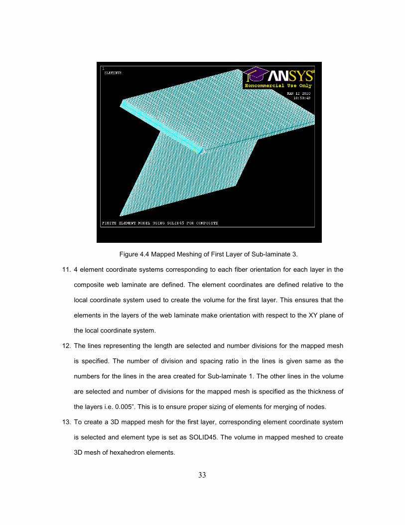
Figure 4.4 Mapped Meshing of First Layer of Sub-laminate 3.

11. 4 element coordinate systems corresponding to each fiber orientation for each layer in the

composite web laminate are defined. The element coordinates are defined relative to the

local coordinate system used to create the volume for the first layer. This ensures that the

elements in the layers of the web laminate make orientation with respect to the XY plane of

the local coordinate system.

12. The lines representing the length are selected and number divisions for the mapped mesh

is specified. The number of division and spacing ratio in the lines is given same as the

numbers for the lines in the area created for Sub-laminate 1. The other lines in the volume

are selected and number of divisions for the mapped mesh is specified as the thickness of

the layers i.e. 0.005”. This is to ensure proper sizing of elements for merging of nodes.

13. To create a 3D mapped mesh for the first layer, corresponding element coordinate system

is selected and element type is set as SOLID45. The volume in mapped meshed to create

3D mesh of hexahedron elements.

34

14. The next layer in web laminate is created by selecting corresponding element coordinate

system and extruding the area at Z=0.005” in the XY plane of local coordinate system. The

other layers in the web are modeled in the similar way to complete the web section.

15. Finally, the Sub-laminate 2 (bottom flange) is modeled using method similar to the method

used to model Sub-laminate 1. To begin, a local coordinate system is defined to represent

the local coordinate system for Sub-laminate 2.

Figure 4.5 Final Finite Element Model.

16. All the nodes and keypoints are merged for adjacent layers faces, which are in contact with

each other. The element sizing and spacing ratio of the elements is of primary importance

for proper merging. The proper merging between layers ensures bonding between them

and continuity of the finite element model. With merging desired finite model is complete.

The final finite element model can be seen in Figure 4.5.

35

4.2.2 Boundary and Loading Condition

The following boundary conditions are applied for the model. Since the finite element

model is used to analyze the cantilever beam condition, all the nodes at X=0 plane is selected

and deflection is all direction is set to zero i.e. Ux=0; Uy=0; Uz=0.

4.3 Validation of Finite Element Model

The finite element model is validated using isotropic properties while maintaining model size,

element orientation and boundary conditions same. The I-beam with 0.5” and 0.75” width of the

top and bottom flanges and 0.5” height of the web laminate (Case 2 I-beam section) was used

to validate the model. The isotropic property used for validation is as follows �� � �� � �� � 1.02 X 10� psi �� � �� � �� � 0.25

!�� � !�� � !�� � ���231 1 ��4 � 4.06 X 10� psi Since the deflection for cantilever beam including its transverse shear deflection at its

free end is well defined, the finite element model is validated using the same condition.

Since the theory used to calculate the end deflection defines the deflection of the beam

at its cross section centroid. For a beam of length of ‘L’ and tip load of ‘P’, the deflection at the

free end can be written as

�� � n �3�¡

And transverse shear deflection can be written as [16]

�� � ¢� n !�

Where ¢� is termed as form factor of shear, and for I-section it is given as

¢� � ��e£�

36

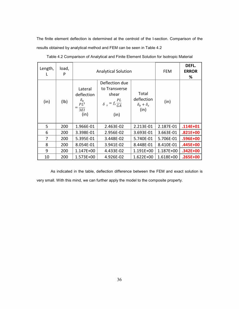
The finite element deflection is determined at the centroid of the I-section. Comparison of the

results obtained by analytical method and FEM can be seen in Table 4.2

Table 4.2 Comparison of Analytical and Finite Element Solution for Isotropic Material

As indicated in the table, deflection difference between the FEM and exact solution is

very small. With this mind, we can further apply the model to the composite property.

Length,

L

load,

P Analytical Solution FEM

DEFL.

ERROR

%

(in) (lb) ��� n �3�¡

Lateral

deflection

(in)

� � � ¢� n !�

Deflection due

to Transverse

shear

(in)

Total

deflection �� 1 ��

(in)

(in)

5 200 1.966E-01 2.463E-02 2.213E-01 2.187E-01 .114E+01

6 200 3.398E-01 2.956E-02 3.693E-01 3.663E-01 .821E+00

7 200 5.395E-01 3.448E-02 5.740E-01 5.706E-01 .596E+00

8 200 8.054E-01 3.941E-02 8.448E-01 8.410E-01 .445E+00

9 200 1.147E+00 4.433E-02 1.191E+00 1.187E+00 .342E+00

10 200 1.573E+00 4.926E-02 1.622E+00 1.618E+00 .265E+00

37

CHAPTER 5

RESULTS FOR CLOSED FORM EXPRESSIONS

This chapter explains in detail the validation results for the analytical expression derived

in Chapter 2. It also compares and analysis the 3 cases of I-section beam under loading.

Finally the stresses along principal axis in the layers on the beam is calculated and analyzed.

5.1 Results Comparison of Centroid Calculation

In this study, the centroid calculation derived in Chapter 2 is validated using the finite

element solution. For the validation, isotropic material properties are chosen as �� � �� � �� � 1.02 X 10� psi �� � �� � �� � 0.25

!�� � !�� � !�� � ���231 1 ��4 � 4.06 X 10� psi After this, composite material is used. The material property of composite materials used is �� � 21.75 @ 10� psi , �� � 1.595 @ 10� psi, �� � 1.595 @ 10� psi

�� � 0.25, �� � 0.45, �� � 0.25, !�� � 0.8702 @ 10� psi , !�� � 0.5366 @ 10� psi , !�� � 0.8702 @ 10� psi

5.1.1 Isotropic Material

The centroid of I-section can be calculated easily, therefore by using isotropic material

property the centroid expression derived for composite material can be validated. Centroid of an

I-section can be calculated using mechanics approach as

38

8 � ∑ �R?RQR∑ �RQR

(5.1) where n is the number divisions of area used to represent the I-section

Table 5.1 lists the results of the centroid calculated using two methods for cases 1, 2 and 3. The

results show an excellent agreement with each other.

Table 5.1 Results for Centroid of I-Section for Isotropic Material

Case Mechanics approach Present Method % Difference

Eq. 5.1 Eq. 3.3

8

(in)

1 0.1421 0.1421 0.0

2 0.2272 0.2272 0.0

3 0.2721 0.2721 0.0

5.1.2 Composite Material

For composite materials, the centroid of the I-section depends on the fiber orientation

and sequence of the layer. The centroid of the section moves between the top and bottom

flange depending on the stiffness of the sub-laminates. With the increase in stiffness of the

bottom flange the centroid moves closer towards bottom flange. Table 5.2 shows the centroid

for various I-sections. The variation of the centroid for various I-section are plotted in Figure 5.1

Table 5.2 Results for Centroid of I-Section for Composite Material

Case Present Method

Eq. 3.3

8

(in)

1 0.1177

2 0.1976

3 0.2424

39

Figure 5.1 Variation of the Centroid along the Z-axis for Different Cases

5.2 Results Comparison for I-Beam Stiffness

The axial and bending stiffnesses of isotropic I-beam are known; therefore the

expression for axial and bending stiffness can be validated by comparing the solution from finite

element model. Two cases of loading were applied to the finite element model to calculate axial

and bending stiffness. An axial load of 200lb was applied at the centroid of the cross-section as

shown in Figure 5.2. The meshing of I-beam was done with extreme care so that a node is

always present at the centroid of the cross-section.

For determining bending stiffness, a pair of forces with the same magnitude but

opposite sign is applied to generate the moment at the centroid; a force of 100lb is applied one

ply away from the centroid of the cross-section. This pair of forces generates a total moment of

0.5 lb-in about the x axis. The pair of force applied on finite element model is shown in Figure

5.3

0.1

0.15

0.2

0.25

0.3

Case 1 Case 2 Case 3

Comparison of centroid for Isotropic and

Composite material

Composite

Isotropic

40

Figure 5.2 J����� Applied at the Centroid of I-section.

Figure 5.3 Pair of Forces Generating T�����.

41

5.2.1 Axial and Bending Stiffnesses of Isotropic Material

The axial stiffness of I-beam was calculated from the finite element model by the

following equation.

������ � ¥ 2i¦�/§C �S¨/�j

(5.2)

Where F is the force applied, L is the total length of the beam, and Ux is the axial deflection. For

all cases, length of the beam is taken as 10 inches.

To avoid any distortion in axial deflection due to the loading or boundary condition, the

deflection results were measured at half way through the length of the beam.

The bending stiffness of I-beam was calculated from the finite element model by

determining the curvature of the beam, �̀ , (See Appendix A) and then dividing the applied

moment by it.

T����� � �� �̀

�� � T������̀

Comparison of the axial and bending stiffnesses for different cases is shown in Table

5.3. The results are excellent agreement with the FEM model. It should be noted that all of I-

beams have thicker bottom flange compared to the upper flange. This results in the higher axial

stiffness and lower bending stiffness for case 1 compared to the other cases.

42

Table 5.3 Comparison of Axial and Bending Stiffnesses of Isotropic I-Beam

CASE UNITS Theoretical Method

Present method % Diff FEM % Diff

1

������ lb 714,000 712,910 -0.15 714,132 0.02

DX lb-in2 30,457 30,405 -0.17 30,507 0.16

2

������ lb 688,500 687,410 -0.16 688,382 -0.02

DX lb-in2 42,381 42,319 -0.15 42,302 -0.19

3

������ lb 680,340 679,240 -0.16 680,170 -0.02

DX lb-in2 44,737 44,668 -0.15 44,360 -0.84

5.2.2 Equivalent Axial and Bending Stiffnesses of Laminated I-Beam

For a laminated I-beam, Table 5.4 lists the comparison of axial and bending stiffnesses

for different I-beams. Same procedure explained above is followed to calculate the axial and

bending for the composite beam.

As expected, equivalent axial stiffness increases and the equivalent bending stiffness

decreases with increase in width of sub-laminate-2 (bottom flange).

Table 5.4 Comparison of Equivalent Axial and Bending Stiffnesses of Laminated I-Beam

CASE UNITS Present method FEM % Diff

1 ������ lb 672,250 664,540 1.16

DX lb-in2 23,886 23,869 0.07

2 ������ lb 618,170 612,040 1.00

DX lb-in2 37,024 36,892 0.36

3 ������ lb 595,460 589,810 0.96

DX lb-in2 40,355 39,659 1.75

43

5.3 Results Comparison of Ply Stresses and Strains of I-Beam

The stresses and strains in plies of sub-laminates of a laminated composite is

calculated using method explained in Chapter 3 with the finite element model. Only one case of

cross-section is considered for the comparison. The stresses in the plies are calculated in their

respective principal coordinate axis i.e. stresses ��, ��, ���.

5.3.1 I-Beam Laminate Ply Stresses under Axial Load, J����� The stresses and strains developed in plies of each sub-laminates due to an axial

loading at the centroid of the cross-section is compared with the analytical solution developed in

Chapter 3. Only Case 2 dimensions of I-section is selected to perform the analysis. The

stresses in plies of the finite element model are obtained in their respective principal coordinate

system. This is done by selecting all the elements of a particular ply and obtaining the stresses

using RSYS command. RSYS command in ANSYS displays the results in particular coordinate

system; local coordinate system of elements in each ply are chosen for obtaining results for the

respective ply. The stresses from analytical expression for each sub laminated are confirmed

from the FEM results (Table 5.5 through Table 5.7).

44

Table 5.5 Comparison of Stresses in Top Flange in Principal Axis due to Axial Load at Centroid

Sigma 1 %Diff Sigma 2 %Diff Tho 12 %Diff

lb/in2 lb/in2 lb/in2

Ply #1 450

Present Method 1260.20 113.40 -183.00

FEM 1344.00 6.24 122.22 7.22 -193.25 5.30

Ply #2 -450

Present Method 1260.20 113.40 183.00

FEM 1348.10 6.52 123.00 7.80 197.34 7.27

Ply #3 00

Present Method 3515.20 -12.90 0.00

FEM 3777.00 6.93 -12.16 -6.10 0.02 exact

Ply #4 &

Ply#5 900

Present Method -994.80 239.80 0.00

FEM -1065.70 6.65 258.49 7.23 0.07 exact

Ply #6 00

Present Method 3515.20 -12.90 0.00

FEM 3782.60 7.07 -13.85 6.86 -0.07 exact

Ply #7 -450

Present Method 1260.20 113.40 183.00

FEM 1357.20 7.15 121.93 7.00 197.22 7.21

Ply #8 450

Present Method 1260.20 113.40 -183.00

FEM 1351.90 6.78 122.10 7.13 -197.48 7.33

45

Table 5.6 Comparison of Stresses in Bottom Flange in Principal Axis due to Axial Load at Centroid

Sigma 1 %Diff Sigma 2 %Diff Tho 12 %Diff

lb/in2 lb/in2 lb/in2

Ply #1 450

Present Method 1263.90 113.80 -182.70

FEM 1239.80 -1.94 111.45 -2.11 -178.50 -2.35

Ply #2 -450

Present Method 1263.90 113.80 182.70

FEM 1238.40 -2.06 111.60 -1.97 178.70 -2.24

Ply #3 & 4 00

Present Method 3515.40 -12.40 0.00

FEM 3444.60 -2.06 -11.91 -4.11 0.05 exact

Ply #5 & 6 900

Present Method -987.60 239.90 0.00

FEM -967.74 -2.05 235.50 -1.87 0.01 exact

Ply #7 & 8 00

Present Method 3515.40 -12.40 0.00

FEM 3456.40 -1.71 -12.22 -1.47 0.03 exact

Ply #9 -450

Present Method 1263.90 113.80 182.70

FEM 1243.80 -1.62 111.83 -1.76 180.08 -1.45

Ply #10 450

Present Method 1263.90 113.80 -182.70

FEM 1242.10 -1.76 111.98 -1.63 -180.30 -1.33

46

Table 5.7 Comparison of Stresses in Web Laminate in Principal Axis due to Axial Load at

Centroid

Sigma 1 %Diff Sigma 2 %Diff Tho 12 %Diff

lb/in2 lb/in2 lb/in2

Ply #1 450

Present Method 451.74 40.66 -246.21

FEM 463.65 2.57 41.45 1.91 -253.67 2.94

Ply #2 -450

Present Method 451.74 40.66 246.21

FEM 462.35 2.29 41.85 2.84 253.55 2.90

Ply #3 -450

Present Method 451.74 40.66 246.21

FEM 464.99 2.85 41.85 2.84 253.42 2.85

Ply #4 -430

Present Method 451.74 40.66 -246.21

FEM 465.65 2.99 42.06 3.33 -253.29 2.80

The percentage increase in transverse and shear stresses is due to exaggeration; in fact the

difference in values is small compared to the axial stress.

5.3.2 I-Beam Laminate Ply Stresses under Bending Moment, T�����

For laminated I-beam the stresses and strains are calculated using the same method as

explained in Section 5.3.1. A moment is generated at the centroid by applying a pair of opposite

axial forces at a distance of one ply from the centroid. The axial stresses and strains perfectly

match with finite element model results. However, again the transverse and shear stresses and

strains are magnified. Table 5.8 through 5.9 shows the comparison of stresses in sub-

laminates.

47

Table 5.8 Comparison of Stresses in Top Flange in Principal Axis due to Bending Moment at Centroid

Sigma 1 %Diff Sigma 2 %Diff Tho 12 %Diff

lb/in2 lb/in2 lb/in2

Ply #1 450

Present Method 38.36 3.41 -5.33

FEM 41.60 7.79 3.84 11.23 -5.24 -1.72

Ply #2 -450

Present Method 38.11 3.46 5.42

FEM 40.55 6.02 3.66 5.36 5.62 3.56

Ply #3 00

Present Method 106.53 -0.33 0.01

FEM 111.01 4.04 -0.31 -5.81 -0.01 225.71

Ply #4 &

Ply#5 900

Present Method -30.11 7.37 0.00

FEM -31.18 3.43 7.70 4.32 0.00 100.00

Ply #6 00

Present Method 110.66 -0.44 0.00

FEM 115.42 4.12 -0.46 5.00 0.00 -37.50

Ply #7 -450

Present Method 39.89 3.57 5.87

FEM 41.35 3.52 3.71 3.83 6.13 4.31

Ply #8 450

Present Method 39.79 3.62 -5.96

FEM 41.42 3.94 3.73 3.08 -6.23 4.41

48

Table 5.9 Comparison of Stresses in Bottom Flange in Principal Axis due to Bending Moment at Centroid

Sigma 1 %Diff Sigma 2 %Diff Tho 12 %Diff

lb/in2 lb/in2 lb/in2

Ply #1 450

Present Method -19.02 -1.74 3.16

FEM -18.40 -3.35 -1.68 -3.76 3.02 -4.54

Ply #2 -450

Present Method -19.18 -1.70 -3.05

FEM -18.44 -4.01 -1.64 -3.66 -2.92 -4.45

Ply #3 & 4 00

Present Method -55.14 0.34 0.01

FEM -52.83 -4.37 0.31 -9.68 0.01 exact

Ply #5 & 6 900

Present Method 15.32 -3.55 0.00

FEM 14.61 -4.86 -3.39 -4.63 0.00 exact

Ply #7 & 8 00

Present Method -47.66 0.07 -0.01

FEM -46.92 -1.57 0.11 37.27 0.00 exact

Ply #9 -450

Present Method -17.48 -1.59 -2.32

FEM -16.61 -5.24 -1.51 -5.40 -2.21 -4.84

Ply #10 450

Present Method -17.57 -1.56 2.21

FEM -16.66 -5.43 -1.50 -3.81 1.93 -14.61

49

5.4 Results Comparison of Ply Stresses in 00 ply in Flange Laminates

The stresses in 00 ply in sub-laminates of I-beam developed due to axial and bending

load is compared for different cases. As expected maximum stress occurs in 00 ply in both

laminates (sub-laminate 1&2).The 00 ply in sub-laminates provide the pure axial stiffness to the

I-beams; therefore the stresses are compared to determine the effect of variation in width of

flange on the stresses in 00 ply of I-beam.

Table 5.10 Comparison of Local Stress in 00 Ply due to Axial Load at Centroid

Top Flange Bottom Flange

psi psi

Case 1 3232.6 3232.6

Case 2 3515.4 3515.2

Case 3 3649.3 3649.4

As expected, the axial stress in 00 ply for both top and bottom flange laminates are equal in

each case.

Table 5.11 Comparison of Local Stress in 00 Ply due to Bending Moment at Centroid

Top Flange Bottom Flange

psi psi

Case 1 207.88 -37.52

Case 2 110.665 -47.656

Case 3 89.47 -55.77

Here again, the stress in 00 ply in the top flange laminate increases and the bottom flange

decreases as the centroid of the cross-section moves down.

50

CHAPTER 6

CONCLUSIVE SUMMARY AND FUTURE WORK

An analytical method was developed for stress analysis of composite I-beam.

Approximate closed-form solution was developed to calculate sectional properties such as

centroid, equivalent axial and bending stiffness. Finally, the stress and strain in each ply of

laminates is calculated using sectional properties. A finite element model is created to obtain

the stiffness of each ply. The results of finite element method were compared with analytical

solution. Three different cross-section configurations were used to compare and validate the

analytical solution.

From this research, following conclusion can be made.

• Analytical expression to calculate centroid shows excellent agreement when validate

using isotropic material.

• Equivalent axial and bending stiffnesses obtained from finite element model showed

excellent agreement with analytical expression for all three configurations.

• The stress and strain in each ply of I-beam subjected to axial and bending load at the

centroid had a difference ranging from negligible to 8% compared to finite element

results.

• The 00 ply in the top and bottom flange laminates had the maximum stresses for both

axial and bending moment loads.

• The axial stress in 00 ply, due to axial load at the centroid, was at its maximum for the I-

beam with equal width of both flanges compared to uneven width of the flanges.

• The axial stress in 00 ply due to bending moment at the centroid was at its maximum for

case 1 compared to others 2 configurations.

51

The new method developed provide excellent alternative for FEM techniques in doing

parametric study. The present method can be extended for composite beam with other cross-

section such as C-beams. The present method can be extended for the I-beam under torsional

load, hygrothermal condition and shear center.

52

APPENDIX A

CALCULATION OF RADIUS OF CURVATURE FROM FINITE ELEMENT MODEL [17]

53

Any three points on a line can be selected to determine the curvature of the line from the finite

element model under bending by using geometrical calculation. Let Points A, B, and C in Figure

A.1 represent three arbitrary points on the line in finite element model with the following

coordinates (x1,y1), (x2,y2), and (x3,y3) respectively.

Figure A.1 Three Points Represented on the Curvature.

The center of the curvature is represented by point O with coordinates (x, y). Using the

coordinates of points A and B the slope and center point of line AB can be defined as

Slope of Line AB,

�s© � =� � =�;� � ;�

Center point P, n3Z�, [�4 � a;� 1 ;�2 , =� 1 =�2 b

O (xo, yo)

L2 L1

R

R

R

Q (a2, b2) P (a1, b1)

A (x1, y1) C (x3, y3)

B (x2, y2)

54

The equation of the line L1 which is perpendicular to line AB at point P can be expressed as

�¨�; � = � �¨�Z� � [�

Where,

�¨� � � 1�ª-«¬ -¢ ª/(¬ �W � � 1�s©

Similarly, using the same procedure the equation of line L2 , perpendicular to line BC at point Q,

can be expressed as

�¨�; � = � �¨�Z� � [�

Where, �¨� � � 1�ª-«¬ -¢ ª/(¬ W, � � 1�©­

J3Z�, [�4 � a;� 1 ;�2 , =� 1 =�2 b

Line L1 and L2 intersect at the center of the curve and the coordinates of point O can be

obtained by solving the equation of lines L1 and L2. The coordinates of center O can be

expressed as

;� � �¨�Z� � �¨�Z� � [� 1 [��¨� � �¨�

=� � �¨��¨�3Z� � Z�4 � �¨�[� 1 �¨�[��¨� � �¨�

The distance from the center point O to any of the points A, B, and C is the radius of the

curvature of the curve ABC. The radius of curvature can be expressed as,

® � ¯3;� � ;�4� 1 3=� � =�4� � ¯3;� � ;�4� 1 3=� � =�4� � ¯3;� � ;�4� 1 3=� � =�4�

A � 1®

55

APPENDIX B

BATCH MODE ANSYS INPUT DATA FILE FOR FINITE ELEMENT MODEL

56

/TITLE,FINITE ELEMENT COMPOSITE MODEL USING SOLID45 /NOPR /PMETH,OFF,0 KEYW,PR_SET,1 KEYW,PR_STRUC,1 KEYW,PR_THERM,0 KEYW,PR_FLUID,0 KEYW,PR_ELMAG,0 KEYW,MAGNOD,0 KEYW,MAGEDG,0 KEYW,MAGHFE,0 KEYW,MAGELC,0 KEYW,PR_MULTI,0 KEYW,PR_CFD,0 ! /PREP7 !------------------------------------------------------- ! MATERIAL PROPERTIES !------------------------------------------------------- MPTEMP,,,,,,,, MPTEMP,1,0 MPDATA,EX,1,,21.75e6 MPDATA,EY,1,,1.595e6 MPDATA,EZ,1,,1.595e6 MPDATA,PRXY,1,,.25 MPDATA,PRYZ,1,,.45 MPDATA,PRXZ,1,,.25 MPDATA,GXY,1,,.8702e6 MPDATA,GYZ,1,,.5366e6 MPDATA,GXZ,1,,.8702e6 ! !------------------------------------------------------- ! MODEL DIMENSION !------------------------------------------------------- L=10 ! LENGTH OF BEAM D=20 ! NO. OF ELEMENT DIVISIONS ON LENGTH OF BEAM F1=0.5 ! WIDTH OF SUB-LAMINATE-1 F2=0.75 ! WIDTH OF SUB-LAMINATE-2 HW=0.5 ! HEIGTH OF SUB-LAMINATE-3 n1=8 ! NO. OF LAYERS IN SUB-LAMINATE-1 n2=10 ! NO. OF LAYERS IN SUB-LAMINATE-2 nw=4 ! NO. OF LAYERS IN SUB-LAMINATE-3 t=0.005 ! THICKNESS OF A LAMINATE PLY ! !------------------------------------------------------- ! ELEMENT SELECTION !------------------------------------------------------- ET,1,PLANE42 ET,2,SOLID45 ! ! !

57

!-------------------------------------------------------------------------------------------------------------- ! LOCAL CORDINATES SYSTEM FOR FIBER ORIENTATION !-------------------------------------------------------------------------------------------------------------- ! !------------------------------------------------------- ! FOR SUB-LAMINATE 1(TOP FLANGE) !------------------------------------------------------- ! LOCAL,11,,0,0,0,45 LOCAL,12,,0,0,0,-45 LOCAL,13,,0,0,0,0 ! LOCAL,14,,0,0,0,90 ! LOCAL,15,,0,0,0,0 LOCAL,16,,0,0,0,-45 LOCAL,17,,0,0,0,45 !------------------------------------------------------- ! FOR SUB-LAMINATE 3 (WEB) !------------------------------------------------------- ! LOCAL,18,0,0,(F1/2-nw*t/2),0,0,-90,0,1,1, ! FOR MODELING AREA CLOCAL,19,0,0,0,0,45 CSYS,18 CLOCAL,20,0,0,0,0,-45 CSYS,18 CLOCAL,21,0,0,0,0,-45 CSYS,18 CLOCAL,22,0,0,0,0,45 CSYS,0 !------------------------------------------------------- ! FOR SUB-LAMINATE 2 (BOTTOM FLANGE) !------------------------------------------------------- ! LOCAL,23,,0,(F1-F2)/2,-(HW+n2*t) ! FOR MODELING AREA LOCAL,24,,0,0,0,45 LOCAL,25,,0,0,0,-45 ! LOCAL,26,,0,0,0,0 ! LOCAL,27,,0,0,0,90 ! LOCAL,28,,0,0,0,0 ! LOCAL,29,,0,0,0,-45 LOCAL,30,,0,0,0,45 CSYS,0 !------------------------------------------------------- ! MODELLING SUB-LAMINATE 1 !------------------------------------------------------- ! K,1,0,0,0,

58

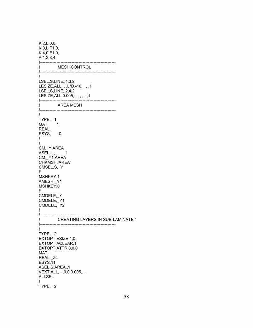
K,2,L,0,0, K,3,L,F1,0, K,4,0,F1,0, A,1,2,3,4 !------------------------------------------------------- ! MESH CONTROL !------------------------------------------------------- ! LSEL,S,LINE,,1,3,2 LESIZE,ALL, , ,L*D,-10, , , ,1 LSEL,S,LINE,,2,4,2 LESIZE,ALL,0.005, , , , , , ,1 !------------------------------------------------------- ! AREA MESH !------------------------------------------------------- ! TYPE, 1 MAT, 1 REAL, ESYS, 0 ! ! CM,_Y,AREA ASEL, , , , 1 CM,_Y1,AREA CHKMSH,'AREA' CMSEL,S,_Y !* MSHKEY,1 AMESH,_Y1 MSHKEY,0 !* CMDELE,_Y CMDELE,_Y1 CMDELE,_Y2 ! !------------------------------------------------------- ! CREATING LAYERS IN SUB-LAMINATE 1 !------------------------------------------------------- ! TYPE, 2 EXTOPT,ESIZE,1,0, EXTOPT,ACLEAR,1 EXTOPT,ATTR,0,0,0 MAT,1 REAL,_Z4 ESYS,11 ASEL,S,AREA,,1 VEXT,ALL, , ,0,0,0.005,,,, ALLSEL ! TYPE, 2

59

EXTOPT,ESIZE,1,0, EXTOPT,ACLEAR,1 EXTOPT,ATTR,0,0,0 MAT,1 REAL,_Z4 ESYS,12 ASEL,S,LOC,Z,0.005 VEXT,ALL, , ,0,0,0.005,,,, ALLSEL ! TYPE, 2 EXTOPT,ESIZE,1,0, EXTOPT,ACLEAR,1 EXTOPT,ATTR,0,0,0 MAT,1 REAL,_Z4 ESYS,13 ASEL,S,LOC,Z,0.01 VEXT,ALL, , ,0,0,0.005,,,, ALLSEL ! TYPE, 2 EXTOPT,ESIZE,1,0, EXTOPT,ACLEAR,1 EXTOPT,ATTR,0,0,0 MAT,1 REAL,_Z4 ESYS,14 ASEL,S,LOC,Z,0.015 VEXT,ALL, , ,0,0,0.01,,,, ALLSEL ! TYPE, 2 EXTOPT,ESIZE,1,0, EXTOPT,ACLEAR,1 EXTOPT,ATTR,0,0,0 MAT,1 REAL,_Z4 ESYS,15 ASEL,S,LOC,Z,0.025 VEXT,ALL, , ,0,0,0.005,,,, ALLSEL ! TYPE, 2 EXTOPT,ESIZE,1,0, EXTOPT,ACLEAR,1 EXTOPT,ATTR,0,0,0 MAT,1 REAL,_Z4 ESYS,16 ASEL,S,LOC,Z,0.03 VEXT,ALL, , ,0,0,0.005,,,,

60

ALLSEL ! ! TYPE, 2 EXTOPT,ESIZE,1,0, EXTOPT,ACLEAR,1 EXTOPT,ATTR,0,0,0 MAT,1 REAL,_Z4 ESYS,17 ASEL,S,LOC,Z,0.035 VEXT,ALL, , ,0,0,0.005,,,, ALLSEL ! !------------------------------------------------------- ! MODELLING SUB-LAMINATE 3 !------------------------------------------------------- CSYS,18 K,33,0,0,0, K,34,L,0,0, K,35,L,HW,0, K,36,0,HW,0, A,33,34,35,36 ! FLST,2,1,5,ORDE,1 FITEM,2,37 VEXT,P51X, , ,0,0,0.005,,,, ! !------------------------------------------------------- ! MESH CONTROL !------------------------------------------------------- LSEL,S,LINE,,61,67,2 LESIZE,ALL, , ,L*D,-10, , , ,1 LSEL,S,LINE,,62,68,2 LESIZE,ALL,0.0025, , , , , , ,1 LSEL,S,LINE,,69,72,1 LESIZE,ALL, , ,1, ,1, , ,1, ! ! ! !------------------------------------------------------- ! CREATING LAYERS IN SUB-LAMINATE 3 !------------------------------------------------------- ! TYPE, 2 MAT, 1 REAL, ESYS, 19 SECNUM, !* CM,_Y,VOLU VSEL, , , , 8

61

CM,_Y1,VOLU CHKMSH,'VOLU' CMSEL,S,_Y !* MSHAPE,0,3d MSHKEY,1 VMESH,_Y1 MSHKEY,0 !* CMDELE,_Y CMDELE,_Y1 CMDELE,_Y2 ! ! TYPE, 2 EXTOPT,ESIZE,1,0, EXTOPT,ACLEAR,1 EXTOPT,ATTR,0,0,0 MAT,1 REAL,_Z4 ESYS,20 ASEL,S,LOC,Z,0.005 VEXT,ALL, , ,0,0,0.005,,,, ALLSEL ! TYPE, 2 EXTOPT,ESIZE,1,0, EXTOPT,ACLEAR,1 EXTOPT,ATTR,0,0,0 MAT,1 REAL,_Z4 ESYS,21 ASEL,S, , , 43 VEXT,ALL, , ,0,0,0.005,,,, ALLSEL ! ! TYPE, 2 EXTOPT,ESIZE,1,0, EXTOPT,ACLEAR,1 EXTOPT,ATTR,0,0,0 MAT,1 REAL,_Z4 ESYS,22 ASEL,S, , , 48 VEXT,ALL, , ,0,0,0.005,,,, ALLSEL ! !------------------------------------------------------- ! MODELLING SUB-LAMINATE 2 !------------------------------------------------------- !

62

CSYS,23 ! K,53,0,0,0, K,54,L,0,0, K,55,L,F2,0, K,56,0,F2,0, A,53,54,55,56 ! !------------------------------------------------------- ! MESH CONTROL !------------------------------------------------------- ! LSEL,S,LINE,,97,99,2 LESIZE,ALL, , ,L*D,-10, , , ,1 LSEL,S,LINE,,98,100,2 LESIZE,ALL,0.005, , , , , , ,1 ! !------------------------------------------------------- ! CREATING LAYERS IN SUB-LAMINATE 3 !------------------------------------------------------- TYPE, 1 MAT, 1 REAL, ESYS, 23 SECNUM, !* CM,_Y,AREA ASEL, , , , 58 CM,_Y1,AREA CHKMSH,'AREA' CMSEL,S,_Y !* !* ACLEAR,_Y1 MSHKEY,1 AMESH,_Y1 MSHKEY,0 !* CMDELE,_Y CMDELE,_Y1 CMDELE,_Y2 ALLSEL ! ! TYPE, 2 EXTOPT,ESIZE,1,0, EXTOPT,ACLEAR,1 EXTOPT,ATTR,0,0,0 MAT,1 REAL,_Z4 ESYS,24 ASEL,S, , , 58

63

VEXT,ALL, , ,0,0,0.005,,,, ALLSEL ! ! TYPE, 2 EXTOPT,ESIZE,1,0, EXTOPT,ACLEAR,1 EXTOPT,ATTR,0,0,0 MAT,1 REAL,_Z4 ESYS,25 ASEL,S, , , 59 VEXT,ALL, , ,0,0,0.005,,,, ALLSEL ! ! TYPE, 2 EXTOPT,ESIZE,1,0, EXTOPT,ACLEAR,1 EXTOPT,ATTR,0,0,0 MAT,1 REAL,_Z4 ESYS,26 ASEL,S, , , 64 VEXT,ALL, , ,0,0,0.01,,,, ALLSEL ! ! TYPE, 2 EXTOPT,ESIZE,1,0, EXTOPT,ACLEAR,1 EXTOPT,ATTR,0,0,0 MAT,1 REAL,_Z4 ESYS,27 ASEL,S, , , 69 VEXT,ALL, , ,0,0,0.01,,,, ALLSEL ! !TYPE, 2 EXTOPT,ESIZE,1,0, EXTOPT,ACLEAR,1 EXTOPT,ATTR,0,0,0 MAT,1 REAL,_Z4 ESYS,28 ASEL,S, , , 74 VEXT,ALL, , ,0,0,0.01,,,, ALLSEL ! ! TYPE, 2

64

EXTOPT,ESIZE,1,0, EXTOPT,ACLEAR,1 EXTOPT,ATTR,0,0,0 MAT,1 REAL,_Z4 ESYS,29 ASEL,S, , , 79 VEXT,ALL, , ,0,0,0.005,,,, ALLSEL ! ! TYPE, 2 EXTOPT,ESIZE,1,0, EXTOPT,ACLEAR,1 EXTOPT,ATTR,0,0,0 MAT,1 REAL,_Z4 ESYS,30 ASEL,S, , , 84 VEXT,ALL, , ,0,0,0.005,,,, ALLSEL ! ! NUMMRG,ALL !MERGE ALL ENTITIES !

65

APPENDIX C

MATLAB CODE FOR ANALYTICAL SOLUTION

66

%%******************************************************************************************************** CALCULATING STRESSES IN LAYERS OF COMPOSITE I-BEAM

%% ******************************************************************************************************* clc clear all %- - - - - - - - - - - - - - - - - - - - - - - - - - - - - - - - - - - - - - - - - - - - - %% MATERIAL PROPERTIES %- - - - - - - - - - - - - - - - - - - - - - - - - - - - - - - - - - - - - - - - - - - - - E1=21.75e6; E2=1.595e6; G12=0.8702e6; V12=0.25; %- - - - - - - - - - - - - - - - - - - - - - - - - - - - - - - - - - - - - - - - - - - - - %% FIBER ORIENTATION %- - - - - - - - - - - - - - - - - - - - - - - - - - - - - - - - - - - - - - - - - - - - - kt=8; % NO. OF LAYERS IN TOP FLANGE kb=10; % NO. OF LAYERS IN BOTTOM FLANGE kw=4; % NO. OF LAYERS IN WEB t=0.005; % THICKNESS OF LAYER % FIBER ORIENTATION IN SUB-LAMINATE-1 theta_fl_f1=pi/180*[45;-45;0;90;90;0;-45;45]; % FIBER ORIENTATION IN SUB-LAMINATE-2 theta_fl_f2=pi/180*[45;-45;0;0;90;90;0;0;-45;45]; % FIBER ORIENTATION IN SUB-LAMINATE-3 theta_w=pi/180*[45;-45;-45;45]; %- - - - - - - - - - - - - - - - - - - - - - - - - - - - - - - - - - - - - - - - - - - - - %% FOR 2D ORTHOTROPIC MATERIAL %- - - - - - - - - - - - - - - - - - - - - - - - - - - - - - - - - - - - - - - - - - - - - S11= 1/E1; S12=-(V12/E1); S22= 1/E2; S66= 1/G12; S=[S11 S12 0 S12 S22 0 0 0 S66]; Q=inv(S); %- - - - - - - - - - - - - - - - - - - - - - - - - - - - - - - - - - - - - - - - - - - - - %% USING LAMINATION THEORY %- - - - - - - - - - - - - - - - - - - - - - - - - - - - - - - - - - - - - - - - - - - - - %% [A], [B], [D] MATRIXES FOR SUB-LAMINATE-1 %- - - - - - - - - - - - - - - - - - - - - - - - - - - - - - - - - - - - - - - - - - - - - A_fl_f1=0; D_fl_f1=zeros(3); B_fl_f1=zeros(3); hkt=zeros(kt+1,1); for i=1:kt m(i,1)=cos(theta_fl_f1(i,1)); n(i,1)=sin(theta_fl_f1(i,1));

67

Q_fl_f1_1_1(i,1)= ((m(i,1)^4)*Q(1,1))+((n(i,1)^4)*Q(2,2))+((2*(Q(1,2)+2*(Q(3,3)))*(m(i,1)*n(i,1))^2)); Q_fl_f1_1_2(i,1)= ((Q(1,1)+Q(2,2)-4*Q(3,3))*((m(i,1)*n(i,1))^2))+((Q(1,2))*(m(i,1)^4+n(i,1)^4)); Q_fl_f1_1_6(i,1)= ((Q(1,1)-Q(1,2)-2*Q(3,3))*((m(i,1))^3)*(n(i,1)))-((Q(2,2)-Q(1,2)-2*Q(3,3))*((n(i,1))^3)*(m(i,1))); Q_fl_f1_2_2(i,1)= (n(i,1)^4)*Q(1,1)+(m(i,1)^4)*Q(2,2)+2*(Q(1,2)+2*Q(3,3))*(m(i,1)*n(i,1))^2; Q_fl_f1_2_6(i,1)= ((Q(1,1)-Q(1,2)-2*Q(3,3))*((n(i,1))^3)*(m(i,1)))-((Q(2,2)-Q(1,2)-2*Q(3,3))*((m(i,1))^3)*(n(i,1))); Q_fl_f1_6_6(i,1)= (Q(1,1)+Q(2,2)-2*Q(1,2)-2*Q(3,3))*(m(i,1)*n(i,1))^2+(Q(3,3))*(m(i,1)^4+n(i,1)^4); Q_f_f1=[Q_fl_f1_1_1(i,1) Q_fl_f1_1_2(i,1) Q_fl_f1_1_6(i,1) Q_fl_f1_1_2(i,1) Q_fl_f1_2_2(i,1) Q_fl_f1_2_6(i,1) Q_fl_f1_1_6(i,1) Q_fl_f1_2_6(i,1) Q_fl_f1_6_6(i,1)] hkt(kt+1,1)=(-kt/2*t); hkt(kt+1-i,1)=(-(kt/2-i)*t); A_fl_f1=A_fl_f1+Q_f_f1*t; B_fl_f1=B_fl_f1+.5*Q_f_f1*(((hkt(kt+1-i,1))^2)-((hkt(kt+2-i,1))^2)); D_fl_f1=D_fl_f1+1/3*Q_f_f1*(((hkt(kt+1-i,1))^3)-((hkt(kt+2-i,1))^3)); end A_fl_f1 B_fl_f1 D_fl_f1 %- - - - - - - - - - - - - - - - - - - - - - - - - - - - - - - - - - - - - - - - - - - - - %% [A], [B], [D] MATRIXES FOR SUB-LAMINATE-2 %- - - - - - - - - - - - - - - - - - - - - - - - - - - - - - - - - - - - - - - - - - - - - A_fl_f2=0; D_fl_f2=zeros(3); B_fl_f2=zeros(3); hkb=zeros(kb+1,1); for i=1:kb m(i,1)=cos(theta_fl_f2(i,1)); n(i,1)=sin(theta_fl_f2(i,1)); Q_fl_f2_1_1(i,1)= ((m(i,1)^4)*Q(1,1))+((n(i,1)^4)*Q(2,2))+((2*(Q(1,2)+2*(Q(3,3)))*(m(i,1)*n(i,1))^2)); Q_fl_f2_1_2(i,1)= ((Q(1,1)+Q(2,2)-4*Q(3,3))*((m(i,1)*n(i,1))^2))+((Q(1,2))*(m(i,1)^4+n(i,1)^4)); Q_fl_f2_1_6(i,1)= ((Q(1,1)-Q(1,2)-2*Q(3,3))*((m(i,1))^3)*(n(i,1)))-((Q(2,2)-Q(1,2)-2*Q(3,3))*((n(i,1))^3)*(m(i,1))); Q_fl_f2_2_2(i,1)= (n(i,1)^4)*Q(1,1)+(m(i,1)^4)*Q(2,2)+2*(Q(1,2)+2*Q(3,3))*(m(i,1)*n(i,1))^2; Q_fl_f2_2_6(i,1)= ((Q(1,1)-Q(1,2)-2*Q(3,3))*((n(i,1))^3)*(m(i,1)))-((Q(2,2)-Q(1,2)-2*Q(3,3))*((m(i,1))^3)*(n(i,1))); Q_fl_f2_6_6(i,1)= (Q(1,1)+Q(2,2)-2*Q(1,2)-2*Q(3,3))*(m(i,1)*n(i,1))^2+(Q(3,3))*(m(i,1)^4+n(i,1)^4); Q_f_f2=[Q_fl_f2_1_1(i,1) Q_fl_f2_1_2(i,1) Q_fl_f2_1_6(i,1) Q_fl_f2_1_2(i,1) Q_fl_f2_2_2(i,1) Q_fl_f2_2_6(i,1) Q_fl_f2_1_6(i,1) Q_fl_f2_2_6(i,1) Q_fl_f2_6_6(i,1)]; hkb(kb+1,1)=(-kb/2*t); hkb(kb+1-i,1)=(-(kb/2-i)*t); A_fl_f2=A_fl_f2+Q_f_f2*t; B_fl_f2=B_fl_f2+.5*Q_f_f2*(((hkb(kb+1-i,1))^2)-((hkb(kb+2-i,1))^2)); D_fl_f2=D_fl_f2+1/3*Q_f_f2*(((hkb(kb+1-i,1))^3)-((hkb(kb+2-i,1))^3));

68

end A_fl_f2 B_fl_f2 D_fl_f2 %- - - - - - - - - - - - - - - - - - - - - - - - - - - - - - - - - - - - - - - - - - - - - %% [A], [B], [D] MATRIXES FOR SUB-LAMINATE-3 %- - - - - - - - - - - - - - - - - - - - - - - - - - - - - - - - - - - - - - - - - - - - - A_w=0; D_w=zeros(3); B_w=zeros(3); hkw=zeros(kw+1,1); for i=1:kw m(i,1)=cos(theta_w(i,1)); n(i,1)=sin(theta_w(i,1)) ; Q_w_1_1(i,1)= ((m(i,1)^4)*Q(1,1))+((n(i,1)^4)*Q(2,2))+((2*(Q(1,2)+2*(Q(3,3)))*(m(i,1)*n(i,1))^2)); Q_w_1_2(i,1)= ((Q(1,1)+Q(2,2)-4*Q(3,3))*((m(i,1)*n(i,1))^2))+((Q(1,2))*(m(i,1)^4+n(i,1)^4)); Q_w_1_6(i,1)= ((Q(1,1)-Q(1,2)-2*Q(3,3))*((m(i,1))^3)*(n(i,1)))-((Q(2,2)-Q(1,2)-2*Q(3,3))*((n(i,1))^3)*(m(i,1))); Q_w_2_2(i,1)= (n(i,1)^4)*Q(1,1)+(m(i,1)^4)*Q(2,2)+2*(Q(1,2)+2*Q(3,3))*(m(i,1)*n(i,1))^2; Q_w_2_6(i,1)= ((Q(1,1)-Q(1,2)-2*Q(3,3))*((n(i,1))^3)*(m(i,1)))-((Q(2,2)-Q(1,2)-2*Q(3,3))*((m(i,1))^3)*(n(i,1))); Q_w_6_6(i,1)= (Q(1,1)+Q(2,2)-2*Q(1,2)-2*Q(3,3))*(m(i,1)*n(i,1))^2+(Q(3,3))*(m(i,1)^4+n(i,1)^4); Q_f_w=[Q_w_1_1(i,1) Q_w_1_2(i,1) Q_w_1_6(i,1) Q_w_1_2(i,1) Q_w_2_2(i,1) Q_w_2_6(i,1) Q_w_1_6(i,1) Q_w_2_6(i,1) Q_w_6_6(i,1)]; hkw(kw+1,1)=(-kw/2*t); hkw(kw+1-i,1)=(-(kw/2-i)*t); A_w=A_w+Q_f_w*t; B_w=B_w+.5*Q_f_w*(((hkw(kw+1-i,1))^2)-((hkw(kw+2-i,1))^2)); D_w=D_w+1/3*Q_f_w*(((hkw(kw+1-i,1))^3)-((hkw(kw+2-i,1))^3)); end A_w B_w D_w %- - - - - - - - - - - - - - - - - - - - - - - - - - - - - - - - - - - - - - - - - - - - - %% CENTROID OF I-SECTION COMPOSITE BEAM %- - - - - - - - - - - - - - - - - - - - - - - - - - - - - - - - - - - - - - - - - - - - - bf_f1=0.5; % BREADTH OF SUB-LAMINATE-1 bf_f2=0.75; % BREADTH OF SUB-LAMINATE-2 hw=0.5; % HEIGTH OF SUB-LAMINATE-3 Z_1=(kb*t)+hw+(0.5*kt*t); Z_2=(0.5*kb*t); Z_3=(kb*t)+(0.5*hw); Z_c_n=((bf_f1*A_fl_f1(1,1)*Z_1)+(bf_f2*A_fl_f2(1,1)*Z_2)+(hw*A_w(1,1)*Z_3)); Z_c_d=((bf_f1*A_fl_f1(1,1))+(bf_f2*A_fl_f2(1,1))+(hw*A_w(1,1))); Z_c=Z_c_n/Z_c_d

69

%- - - - - - - - - - - - - - - - - - - - - - - - - - - - - - - - - - - - - - - - - - - - - - - - - - - - - - - - - - - - - - - - - - - - %% EQUVALENT AXIAL STIFFNESS %- - - - - - - - - - - - - - - - - - - - - - - - - - - - - - - - - - - - - - - - - - - - - - - - - - - - - - - - - - - - - - - - - - - - EA1=((bf_f1*A11_str_f1)+(bf_f2*A11_str_f2)+(hw*A11_str_w)) %- - - - - - - - - - - - - - - - - - - - - - - - - - - - - - - - - - - - - - - - - - - - - - - - - - - - - - - - - - - - - - - - - - - - %% EQUIVALENT BENDING STIFFNESS %- - - - - - - - - - - - - - - - - - - - - - - - - - - - - - - - - - - - - - - - - - - - - - - - - - - - - - - - - - - - - - - - - - - - Z_1c=Z_1-Z_c % DISTANCE BETWEEN MID-PLANE OF SUB-LAMINATE-1 & CENTRIOD Z_2c=(Z_2-Z_c) % DISTANCE BETWEEN MID-PLANE OF SUB-LAMINATE-2 & CENTRIOD hwc=Z_3-Z_c % DISTANCE BETWEEN MID-PLANE OF SUB-LAMINATE-3 & CENTRIOD mx1=bf_f1*((A11_str_f1*Z_1c^2)+(B11_str_f1*2*Z_1c)+(D11_str_f1)); mx2=bf_f2*((A11_str_f2*Z_2c^2)+(B11_str_f2*2*Z_2c)+(D11_str_f2)); mx3=A11_str_w*((1/12*(hw^3))+(hw*(hwc^2))); DX1=mx1+mx2+mx3 %- - - - - - - - - - - - - - - - - - - - - - - - - - - - - - - - - - - - - - - - - - - - - %% CONSTITUTIVE EQUATION OF NARROW BEAM %- - - - - - - - - - - - - - - - - - - - - - - - - - - - - - - - - - - - - - - - - - - - - %% FOR SUB-LAMINATE 1 %- - - - - - - - - - - - - - - - - - - - - - - - - - - - - - - - - - - - - - - - - - - - - K_f1=zeros(6); K_f1=[A_fl_f1 B_fl_f1;B_fl_f1 D_fl_f1]; K_f1_tr=inv(K_f1); a_f1=K_f1_tr(1:3,1:3); b_f1=K_f1_tr(1:3,4:6); b_t_f1=K_f1_tr(4:6,1:3); d_f1=K_f1_tr(4:6,4:6); a11_f1=a_f1(1:1,1:1); b11_f1=b_f1(1:1,1:1); b_t11_f1=b_t_f1(1:1,1:1); d11_f1=d_f1(1:1,1:1); K1_f1=[a11_f1 b11_f1 b_t11_f1 d11_f1]; K1_t_f1=inv(K1_f1); A11_str_f1=K1_t_f1(1,1); B11_str_f1=K1_t_f1(1,2); D11_str_f1=K1_t_f1(2,2); %- - - - - - - - - - - - - - - - - - - - - - - - - - - - - - - - - - - - - - - - - - - - - %% FOR SUB-LAMINATE 2 %- - - - - - - - - - - - - - - - - - - - - - - - - - - - - - - - - - - - - - - - - - - - -

70

K_f2=zeros(6); K_f2=[A_fl_f2 B_fl_f2;B_fl_f2 D_fl_f2]; K_f2_tr=inv(K_f2); a_f2=K_f2_tr(1:3,1:3); b_f2=K_f2_tr(1:3,4:6); b_t_f2=K_f2_tr(4:6,1:3); d_f2=K_f2_tr(4:6,4:6); a11_f2=a_f2(1:1,1:1); b11_f2=b_f2(1:1,1:1); b_t11_f2=b_t_f2(1:1,1:1); d11_f2=d_f2(1:1,1:1); K1_f2=[a11_f2 b11_f2 b_t11_f2 d11_f2]; K1_t_f2=inv(K1_f2); A11_str_f2=K1_t_f2(1,1); B11_str_f2=K1_t_f2(1,2); D11_str_f2=K1_t_f2(2,2); %- - - - - - - - - - - - - - - - - - - - - - - - - - - - - - - - - - - - - - - - - - - - - %% FOR SUB-LAMINATE-3 %- - - - - - - - - - - - - - - - - - - - - - - - - - - - - - - - - - - - - - - - - - - - - K_w=zeros(6); K_w=[A_w B_w;B_w D_w]; K_w_tr=inv(K_w); a_w=K_w_tr(1:3,1:3); b_w=K_w_tr(1:3,4:6); b_t_w=K_w_tr(4:6,1:3); d_w=K_w_tr(4:6,4:6); a11_w=a_w(1:1,1:1); b11_w=b_w(1:1,1:1); b_t11_w=b_t_w(1:1,1:1); d11_w=d_w(1:1,1:1); K1_w=[a11_w b11_w b_t11_w d11_w]; K1_t_w=inv(K1_w); A11_str_w=K1_t_w(1,1); B11_str_w=K1_t_w(1,2); D11_str_w=K1_t_w(2,2); %- - - - - - - - - - - - - - - - - - - - - - - - - - - - - - - - - - - - - - - - - - - - - - - - - - - - - - - - - - - - - - - - - - - - %% STRESSES AND STRAINS IN LAMINATES LAYERS DUE TO MOMENT, M ACTING AT % THE CENTRIOD %- - - - - - - - - - - - - - - - - - - - - - - - - - - - - - - - - - - - - - - - - - - - - - - - - - - - - - - - - - - - - - - - - - - - M=0.5 %- - - - - - - - - - - - - - - - - - - - - - - - - - - - - - - - - - - - - - - - - - - - - %% SECTIONAL PROPERTIES %- - - - - - - - - - - - - - - - - - - - - - - - - - - - - - - - - - - - - - - - - - - - - EA1 =6.1817e+005 % AXIAL STIFFNESS DX1 =3.7024e+004 %BENDING STIFFNESS K_x_c=M/DX1 % MID-PLANE STRAIN AT CENTRIOD

71

Z_1c=Z_1-Z_c % DISTANCE BTW MID-PLANE OF SUB-LAMINATE-1 & CENTRIOD Z_2c=(Z_2-Z_c) % DISTANCE BTW MID-PLANE OF SUB-LAMINATE-2 & CENTRIOD hwc=Z_3-Z_c % DISTANCE BTW MID-PLANE OF SUB-LAMINATE-3 & CENTRIOD %- - - - - - - - - - - - - - - - - - - - - - - - - - - - - - - - - - - - - - - - - - - - - %% FOR SUB-LAMINATES 1 %- - - - - - - - - - - - - - - - - - - - - - - - - - - - - - - - - - - - - - - - - - - - - % Force and Moments Nx_1_f1=(B11_str_f1+(Z_1c*A11_str_f1))*K_x_c; Mx_1_f1=(D11_str_f1+(Z_1c*B11_str_f1))*K_x_c; Mxy_1_f1=(1/d_f1(3,3))*((b_t_f1(1,3)*Nx_1_f1)+(d_f1(1,3)*Mx_1_f1)); F_0_f1=[Nx_1_f1;Mx_1_f1;Mxy_1_f1]; % % Mid-plane strains and curvature Ep_0_f1=zeros(3,3); Ep_0_f1(:,1)=K_f1_tr(1:3,1:1); Ep_0_f1(:,2)=K_f1_tr(1:3,4:4); Ep_0_f1(:,3)=K_f1_tr(1:3,5:5); Ep_0_f1=Ep_0_f1*F_0_f1; K_0_f1=zeros(3,3); K_0_f1(:,1)=K_f1_tr(4:6,1:1); K_0_f1(:,2)=K_f1_tr(4:6,4:4); K_0_f1(:,3)=K_f1_tr(4:6,5:5); K_0_f1=K_0_f1*F_0_f1; Ep_k_f1=zeros(3,kt+1); Sigma_k_f1=zeros(3,kt+1); for i=1:kt Z_kt=hkt(kt+2-i,1); Ep_k_f1(:,kt+2-i)=Ep_0_f1+(Z_kt*K_0_f1) m1=theta_fl_f1(i,1); n1=theta_fl_f1(i,1); m=cos(m1); n=sin(n1); Q_fl_f1_1_1= ((m^4)*Q(1,1))+((n^4)*Q(2,2))+((2*(Q(1,2)+2*(Q(3,3)))*(m*n)^2)); Q_fl_f1_1_2= ((Q(1,1)+Q(2,2)-4*Q(3,3))*((m*n)^2))+((Q(1,2))*(m^4+n^4)); Q_fl_f1_1_6= ((Q(1,1)-Q(1,2)-2*Q(3,3))*((m)^3)*(n))-((Q(2,2)-Q(1,2)-2*Q(3,3))*((n)^3)*(m)); Q_fl_f1_2_2= (n^4)*Q(1,1)+(m^4)*Q(2,2)+2*(Q(1,2)+2*Q(3,3))*(m*n)^2; Q_fl_f1_2_6= ((Q(1,1)-Q(1,2)-2*Q(3,3))*((n)^3)*(m))-((Q(2,2)-Q(1,2)-2*Q(3,3))*((m)^3)*(n)); Q_fl_f1_6_6= (Q(1,1)+Q(2,2)-2*Q(1,2)-2*Q(3,3))*(m*n)^2+(Q(3,3))*(m^4+n^4); Q_f_f1=[Q_fl_f1_1_1 Q_fl_f1_1_2 Q_fl_f1_1_6 Q_fl_f1_1_2 Q_fl_f1_2_2 Q_fl_f1_2_6 Q_fl_f1_1_6 Q_fl_f1_2_6 Q_fl_f1_6_6]; Sigma_k_f1(:,kt+2-i)= Q_f_f1*Ep_k_f1(1:3,kt+2-i:kt+2-i); end Z_kt=hkt(1,1); Ep_k_f1(:,1)=Ep_0_f1+(Z_kt*K_0_f1); Sigma_k_f1(:,1)= Q_f_f1*Ep_k_f1(1:3,1:1);

72

%- - - - - - - - - - - - - - - - - - - - - - - - - - - - - - - - - - - - - - - - - - - - - %% FOR SUB-LAMINATES-2 %- - - - - - - - - - - - - - - - - - - - - - - - - - - - - - - - - - - - - - - - - - - - - % Force and Moments Nx_1_f2=(B11_str_f2+Z_2c*A11_str_f2)*K_x_c; Mx_1_f2=(D11_str_f2+Z_2c*B11_str_f2)*K_x_c; Mxy_1_f2=(1/d_f2(3,3))*((b_t_f2(1,3)*Nx_1_f2)+(d_f2(1,3)*Mx_1_f2)); F_0_f2=[Nx_1_f2;Mx_1_f2;Mxy_1_f2]; % Mid-plane strains and curvature Ep_0_f2=zeros(3,3); Ep_0_f2(:,1)=K_f2_tr(1:3,1:1); Ep_0_f2(:,2)=K_f2_tr(1:3,4:4); Ep_0_f2(:,3)=K_f2_tr(1:3,5:5); Ep_0_f2=Ep_0_f2*F_0_f2; K_0_f2=zeros(3,3); K_0_f2(:,1)=K_f2_tr(4:6,1:1); K_0_f2(:,2)=K_f2_tr(4:6,4:4); K_0_f2(:,3)=K_f2_tr(4:6,5:5); K_0_f2=K_0_f2*F_0_f2; Ep_k_f2=zeros(3,kb+1); Sigma_k_f2=zeros(3,kb+1); for i=1:kb Z_kb=hkb(kb+2-i,1); Ep_k_f2(:,kb+2-i)=Ep_0_f2+(Z_kb*K_0_f2); m2=theta_fl_f2(i,1); n2=theta_fl_f2(i,1); m=cos(m2); n=sin(n2); Q_fl_f2_1_1= ((m^4)*Q(1,1))+((n^4)*Q(2,2))+((2*(Q(1,2)+2*(Q(3,3)))*(m*n)^2)); Q_fl_f2_1_2= ((Q(1,1)+Q(2,2)-4*Q(3,3))*((m*n)^2))+((Q(1,2))*(m^4+n^4)); Q_fl_f2_1_6= ((Q(1,1)-Q(1,2)-2*Q(3,3))*((m)^3)*(n))-((Q(2,2)-Q(1,2)-2*Q(3,3))*((n)^3)*(m)); Q_fl_f2_2_2= (n^4)*Q(1,1)+(m^4)*Q(2,2)+2*(Q(1,2)+2*Q(3,3))*(m*n)^2; Q_fl_f2_2_6= ((Q(1,1)-Q(1,2)-2*Q(3,3))*((n)^3)*(m))-((Q(2,2)-Q(1,2)-2*Q(3,3))*((m)^3)*(n)); Q_fl_f2_6_6= (Q(1,1)+Q(2,2)-2*Q(1,2)-2*Q(3,3))*(m*n)^2+(Q(3,3))*(m^4+n^4); Q_f_f2=[Q_fl_f2_1_1 Q_fl_f2_1_2 Q_fl_f2_1_6 Q_fl_f2_1_2 Q_fl_f2_2_2 Q_fl_f2_2_6 Q_fl_f2_1_6 Q_fl_f2_2_6 Q_fl_f2_6_6]; Sigma_k_f2(:,kb+2-i)= Q_f_f2*Ep_k_f2(1:3,kb+2-i:kb+2-i); end Z_kt=hkb(1,1); Ep_k_f2(:,1)=Ep_0_f2+(Z_kt*K_0_f2); Sigma_k_f2(:,1)= Q_f_f2*Ep_k_f2(1:3,1:1); %- - - - - - - - - - - - - - - - - - - - - - - - - - - - - - - - - - - - - - - - - - - - - %% FOR WEB-LAMINATE-3 %- - - - - - - - - - - - - - - - - - - - - - - - - - - - - - - - - - - - - - - - - - - - -

73

% Force and Moments Nx_1_w=(B11_str_w+hwc*A11_str_w)*K_x_c; Mx_1_w=(D11_str_w+hwc*B11_str_w)*K_x_c; Mxy_1_w=(1/d_w(3,3))*((b_t_w(1,3)*Nx_1_w)+(d_w(1,3)*Mx_1_w)); F_0_w=[Nx_1_w;Mx_1_w;Mxy_1_w]; % Mid-plane strains and curvature Ep_0_w=zeros(3,3); Ep_0_w(:,1)=K_w_tr(1:3,1:1); Ep_0_w(:,2)=K_w_tr(1:3,4:4); Ep_0_w(:,3)=K_w_tr(1:3,5:5); Ep_0_w=Ep_0_w*F_0_w; K_0_w=zeros(3,3); K_0_w(:,1)=K_w_tr(4:6,1:1); K_0_w(:,2)=K_w_tr(4:6,4:4); K_0_w(:,3)=K_w_tr(4:6,5:5); K_0_w=K_0_w*F_0_w; Ep_k_w=zeros(3,kw+1); Sigma_k_w=zeros(3,kw+1); for i=1:kw Z_kw=hkw(i+1,1); Ep_k_w(:,kw+2-i)=Ep_0_w+(Z_kw*K_0_w); m2=theta_w(i,1); n2=theta_w(i,1); m=cos(m2); n=sin(n2); Q_fl_w_1_1= ((m^4)*Q(1,1))+((n^4)*Q(2,2))+((2*(Q(1,2)+2*(Q(3,3)))*(m*n)^2)); Q_fl_w_1_2= ((Q(1,1)+Q(2,2)-4*Q(3,3))*((m*n)^2))+((Q(1,2))*(m^4+n^4)); Q_fl_w_1_6= ((Q(1,1)-Q(1,2)-2*Q(3,3))*((m)^3)*(n))-((Q(2,2)-Q(1,2)-2*Q(3,3))*((n)^3)*(m)); Q_fl_w_2_2= (n^4)*Q(1,1)+(m^4)*Q(2,2)+2*(Q(1,2)+2*Q(3,3))*(m*n)^2; Q_fl_w_2_6= ((Q(1,1)-Q(1,2)-2*Q(3,3))*((n)^3)*(m))-((Q(2,2)-Q(1,2)-2*Q(3,3))*((m)^3)*(n)); Q_fl_w_6_6= (Q(1,1)+Q(2,2)-2*Q(1,2)-2*Q(3,3))*(m*n)^2+(Q(3,3))*(m^4+n^4); Q_f_w=[Q_fl_w_1_1 Q_fl_w_1_2 Q_fl_w_1_6 Q_fl_w_1_2 Q_fl_w_2_2 Q_fl_w_2_6 Q_fl_w_1_6 Q_fl_w_2_6 Q_fl_w_6_6]; Sigma_k_w(:,kw+2-i)= Q_f_w*Ep_k_w(1:3,kw+2-i:kw+2-i); end Z_kt=hkw(1,1); Ep_k_w(:,1)=Ep_0_w+(Z_kt*K_0_w); Sigma_k_w(:,1)= Q_f_w*Ep_k_w(1:3,1:1); %- - - - - - - - - - - - - - - - - - - - - - - - - - - - - - - - - - - - - - - - - - - - - - - - - - - - - - - - - - - - - - - - - - - - %% STRESSES IN PRINCIPAL COORDINATES SYSTEM %- - - - - - - - - - - - - - - - - - - - - - - - - - - - - - - - - - - - - - - - - - - - - - - - - - - - - - - - - - - - - - - - - - - - Sigma_k_f1_pr=zeros(3,kt); Sigma_k_f2_pr=zeros(3,kb);

74

Sigma_k_w_pr=zeros(3,kw); %- - - - - - - - - - - - - - - - - - - - - - - - - - - - - - - - - - - - - - - - - - - - - %% SUB-LAMINATE-1 %- - - - - - - - - - - - - - - - - - - - - - - - - - - - - - - - - - - - - - - - - - - - - for i=1:kt m2=theta_fl_f1(i,1); n2=theta_fl_f1(i,1); m=cos(m2); n=sin(n2); T_Sigma=[m^2 n^2 2*m*n n^2 m^2 -2*m*n -m*n m*n (m^2-n^2)]; Sigma_k_f1_pr(:,i)=T_Sigma*Sigma_k_f1(:,i); end %- - - - - - - - - - - - - - - - - - - - - - - - - - - - - - - - - - - - - - - - - - - - - % SUB-LAMINATE-2 %- - - - - - - - - - - - - - - - - - - - - - - - - - - - - - - - - - - - - - - - - - - - - for i=1:kb m2=theta_fl_f2(i,1); n2=theta_fl_f2(i,1); m=cos(m2); n=sin(n2); T_Sigma=[m^2 n^2 2*m*n n^2 m^2 -2*m*n -m*n m*n (m^2-n^2)]; Sigma_k_f2_pr(:,i+1)=T_Sigma*Sigma_k_f2(:,i+1); end %- - - - - - - - - - - - - - - - - - - - - - - - - - - - - - - - - - - - - - - - - - - - - % SUB-LAMINATE-3 %- - - - - - - - - - - - - - - - - - - - - - - - - - - - - - - - - - - - - - - - - - - - - for i=1:kw m2=theta_w(i,1); n2=theta_w(i,1); m=cos(m2); n=sin(n2); T_Sigma=[m^2 n^2 2*m*n n^2 m^2 -2*m*n -m*n m*n (m^2-n^2)]; Sigma_k_w_pr(:,i+1)=T_Sigma*Sigma_k_w(:,i+1); end %- - - - - - - - - - - - - - - - - - - - - - - - - - - - - - - - - - - - - - - - - - - - - - - - - - - - - - - - - - - - - - - - - - - - %% VIEWING RESULTS %- - - - - - - - - - - - - - - - - - - - - - - - - - - - - - - - - - - - - - - - - - - - - - - - - - - - - - - - - - - - - - - - - - - - %- - - - - - - - - - - - - - - - - - - - - - - - - - - - - - - - - - - - - - - - - - - - - % STRESSES IN LAYERS SUB-LAMINATE-1 (GLOBAL AND LOCAL COORDINATES) %- - - - - - - - - - - - - - - - - - - - - - - - - - - - - - - - - - - - - - - - - - - - -

75

Sigma_k_f1 Sigma_k_f1_pr %- - - - - - - - - - - - - - - - - - - - - - - - - - - - - - - - - - - - - - - - - - - - - % STRESSES IN LAYERS SUB-LAMINATE-2 (GLOBAL AND LOCAL COORDINATES) %- - - - - - - - - - - - - - - - - - - - - - - - - - - - - - - - - - - - - - - - - - - - - Sigma_k_f2 Sigma_k_f2_pr %- - - - - - - - - - - - - - - - - - - - - - - - - - - - - - - - - - - - - - - - - - - - - % STRESSES IN LAYERS SUB-LAMINATE-3 (GLOBAL AND LOCAL COORDINATES) %- - - - - - - - - - - - - - - - - - - - - - - - - - - - - - - - - - - - - - - - - - - - - Sigma_k_w Sigma_k_w_pr

%- - - - - - - - - - - - - - - - - - - - - - - - - - - - - - - - - - - - - - - - - - - - - - - - - - - - - - - - - - - - - - - - - - - - %% STRESSES AND STRAINS IN LAMINATES LAYERS DUE TO AXIAL LOAD, PX % ACTING AT THE CENTRIOD %- - - - - - - - - - - - - - - - - - - - - - -- - - - - - - - - - - - - - - - - - - - - - - - - - - - - - - - - - - - - - - - - - - - - P=100 Ep_x_c=P/EA1 % MID-PLANE STRAIN AT CENTRIOD %- - - - - - - - - - - - - - - - - - - - - - - - - - - - - - - - - - - - - - - - - - - - - %% FOR SUB-LAMINATES 1 %- - - - - - - - - - - - - - - - - - - - - - - - - - - - - - - - - - - - - - - - - - - - - % Force and Moments Nx_1_f1=(A11_str_f1)*Ep_x_c Mx_1_f1=(B11_str_f1)*Ep_x_c Mxy_1_f1=(1/d_f1(3,3))*((b_t_f1(1,3)*Nx_1_f1)+(d_f1(1,3)*Mx_1_f1)) F_0_f1=[Nx_1_f1;Mx_1_f1;Mxy_1_f1] % % Mid-plane strains and curvature Ep_0_f1=zeros(3,3); Ep_0_f1(:,1)=K_f1_tr(1:3,1:1); Ep_0_f1(:,2)=K_f1_tr(1:3,4:4); Ep_0_f1(:,3)=K_f1_tr(1:3,5:5); Ep_0_f1=Ep_0_f1*F_0_f1; K_0_f1=zeros(3,3); K_0_f1(:,1)=K_f1_tr(4:6,1:1); K_0_f1(:,2)=K_f1_tr(4:6,4:4); K_0_f1(:,3)=K_f1_tr(4:6,5:5); K_0_f1=K_0_f1*F_0_f1; Ep_k_f1=zeros(3,kt+1); Sigma_k_f1=zeros(3,kt+1);

76

for i=1:kt Z_kt=hkt(kt+2-i,1); Ep_k_f1(:,kt+2-i)=Ep_0_f1+(Z_kt*K_0_f1) m1=theta_fl_f1(i,1); n1=theta_fl_f1(i,1); m=cos(m1); n=sin(n1); Q_fl_f1_1_1= ((m^4)*Q(1,1))+((n^4)*Q(2,2))+((2*(Q(1,2)+2*(Q(3,3)))*(m*n)^2)); Q_fl_f1_1_2= ((Q(1,1)+Q(2,2)-4*Q(3,3))*((m*n)^2))+((Q(1,2))*(m^4+n^4)); Q_fl_f1_1_6= ((Q(1,1)-Q(1,2)-2*Q(3,3))*((m)^3)*(n))-((Q(2,2)-Q(1,2)-2*Q(3,3))*((n)^3)*(m)); Q_fl_f1_2_2= (n^4)*Q(1,1)+(m^4)*Q(2,2)+2*(Q(1,2)+2*Q(3,3))*(m*n)^2; Q_fl_f1_2_6= ((Q(1,1)-Q(1,2)-2*Q(3,3))*((n)^3)*(m))-((Q(2,2)-Q(1,2)-2*Q(3,3))*((m)^3)*(n)); Q_fl_f1_6_6= (Q(1,1)+Q(2,2)-2*Q(1,2)-2*Q(3,3))*(m*n)^2+(Q(3,3))*(m^4+n^4); Q_f_f1=[Q_fl_f1_1_1 Q_fl_f1_1_2 Q_fl_f1_1_6 Q_fl_f1_1_2 Q_fl_f1_2_2 Q_fl_f1_2_6 Q_fl_f1_1_6 Q_fl_f1_2_6 Q_fl_f1_6_6]; Sigma_k_f1(:,kt+2-i)= Q_f_f1*Ep_k_f1(1:3,kt+2-i:kt+2-i); end Z_kt=hkt(1,1); Ep_k_f1(:,1)=Ep_0_f1+(Z_kt*K_0_f1); Sigma_k_f1(:,1)= Q_f_f1*Ep_k_f1(1:3,1:1); %- - - - - - - - - - - - - - - - - - - - - - - - - - - - - - - - - - - - - - - - - - - - - %% FOR SUB-LAMINATES-2 %- - - - - - - - - - - - - - - - - - - - - - - - - - - - - - - - - - - - - - - - - - - - - % Force and Moments Nx_1_f2=(A11_str_f2)*Ep_x_c; Mx_1_f2=(B11_str_f2)*Ep_x_c; Mxy_1_f2=(1/d_f2(3,3))*((b_t_f2(1,3)*Nx_1_f2)+(d_f2(1,3)*Mx_1_f2)); F_0_f2=[Nx_1_f2;Mx_1_f2;Mxy_1_f2]; % Mid-plane strains and curvature Ep_0_f2=zeros(3,3); Ep_0_f2(:,1)=K_f2_tr(1:3,1:1); Ep_0_f2(:,2)=K_f2_tr(1:3,4:4); Ep_0_f2(:,3)=K_f2_tr(1:3,5:5); Ep_0_f2=Ep_0_f2*F_0_f2; K_0_f2=zeros(3,3); K_0_f2(:,1)=K_f2_tr(4:6,1:1); K_0_f2(:,2)=K_f2_tr(4:6,4:4); K_0_f2(:,3)=K_f2_tr(4:6,5:5); K_0_f2=K_0_f2*F_0_f2; Ep_k_f2=zeros(3,kb+1); Sigma_k_f2=zeros(3,kb+1); for i=1:kb Z_kb=hkb(kb+2-i,1); Ep_k_f2(:,kb+2-i)=Ep_0_f2+(Z_kb*K_0_f2);

77

m2=theta_fl_f2(i,1); n2=theta_fl_f2(i,1); m=cos(m2); n=sin(n2); Q_fl_f2_1_1= ((m^4)*Q(1,1))+((n^4)*Q(2,2))+((2*(Q(1,2)+2*(Q(3,3)))*(m*n)^2)); Q_fl_f2_1_2= ((Q(1,1)+Q(2,2)-4*Q(3,3))*((m*n)^2))+((Q(1,2))*(m^4+n^4)); Q_fl_f2_1_6= ((Q(1,1)-Q(1,2)-2*Q(3,3))*((m)^3)*(n))-((Q(2,2)-Q(1,2)-2*Q(3,3))*((n)^3)*(m)); Q_fl_f2_2_2= (n^4)*Q(1,1)+(m^4)*Q(2,2)+2*(Q(1,2)+2*Q(3,3))*(m*n)^2; Q_fl_f2_2_6= ((Q(1,1)-Q(1,2)-2*Q(3,3))*((n)^3)*(m))-((Q(2,2)-Q(1,2)-2*Q(3,3))*((m)^3)*(n)); Q_fl_f2_6_6= (Q(1,1)+Q(2,2)-2*Q(1,2)-2*Q(3,3))*(m*n)^2+(Q(3,3))*(m^4+n^4); Q_f_f2=[Q_fl_f2_1_1 Q_fl_f2_1_2 Q_fl_f2_1_6 Q_fl_f2_1_2 Q_fl_f2_2_2 Q_fl_f2_2_6 Q_fl_f2_1_6 Q_fl_f2_2_6 Q_fl_f2_6_6]; Sigma_k_f2(:,kb+2-i)= Q_f_f2*Ep_k_f2(1:3,kb+2-i:kb+2-i); end Z_kt=hkb(1,1); Ep_k_f2(:,1)=Ep_0_f2+(Z_kt*K_0_f2); Sigma_k_f2(:,1)= Q_f_f2*Ep_k_f2(1:3,1:1); %- - - - - - - - - - - - - - - - - - - - - - - - - - - - - - - - - - - - - - - - - - - - - %% FOR WEB-LAMINATE-3 %- - - - - - - - - - - - - - - - - - - - - - - - - - - - - - - - - - - - - - - - - - - - - % Force and Moments Nx_1_w=(A11_str_w)*Ep_x_c; Mx_1_w=(B11_str_w)*Ep_x_c; Mxy_1_w=(1/d_w(3,3))*((b_t_w(1,3)*Nx_1_w)+(d_w(1,3)*Mx_1_w)); F_0_w=[Nx_1_w;Mx_1_w;Mxy_1_w]; % Mid-plane strains and curvature Ep_0_w=zeros(3,3); Ep_0_w(:,1)=K_w_tr(1:3,1:1); Ep_0_w(:,2)=K_w_tr(1:3,4:4); Ep_0_w(:,3)=K_w_tr(1:3,5:5); Ep_0_w=Ep_0_w*F_0_w; K_0_w=zeros(3,3); K_0_w(:,1)=K_w_tr(4:6,1:1); K_0_w(:,2)=K_w_tr(4:6,4:4); K_0_w(:,3)=K_w_tr(4:6,5:5); K_0_w=K_0_w*F_0_w; Ep_k_w=zeros(3,kw+1); Sigma_k_w=zeros(3,kw+1); for i=1:kw Z_kw=hkw(i+1,1); Ep_k_w(:,kw+2-i)=Ep_0_w+(Z_kw*K_0_w); m2=theta_w(i,1); n2=theta_w(i,1); m=cos(m2); n=sin(n2);

78

Q_fl_w_1_1= ((m^4)*Q(1,1))+((n^4)*Q(2,2))+((2*(Q(1,2)+2*(Q(3,3)))*(m*n)^2)); Q_fl_w_1_2= ((Q(1,1)+Q(2,2)-4*Q(3,3))*((m*n)^2))+((Q(1,2))*(m^4+n^4)); Q_fl_w_1_6= ((Q(1,1)-Q(1,2)-2*Q(3,3))*((m)^3)*(n))-((Q(2,2)-Q(1,2)-2*Q(3,3))*((n)^3)*(m)); Q_fl_w_2_2= (n^4)*Q(1,1)+(m^4)*Q(2,2)+2*(Q(1,2)+2*Q(3,3))*(m*n)^2; Q_fl_w_2_6= ((Q(1,1)-Q(1,2)-2*Q(3,3))*((n)^3)*(m))-((Q(2,2)-Q(1,2)-2*Q(3,3))*((m)^3)*(n)); Q_fl_w_6_6= (Q(1,1)+Q(2,2)-2*Q(1,2)-2*Q(3,3))*(m*n)^2+(Q(3,3))*(m^4+n^4); Q_f_w=[Q_fl_w_1_1 Q_fl_w_1_2 Q_fl_w_1_6 Q_fl_w_1_2 Q_fl_w_2_2 Q_fl_w_2_6 Q_fl_w_1_6 Q_fl_w_2_6 Q_fl_w_6_6]; Sigma_k_w(:,kw+2-i)= Q_f_w*Ep_k_w(1:3,kw+2-i:kw+2-i); end Z_kt=hkw(1,1); Ep_k_w(:,1)=Ep_0_w+(Z_kt*K_0_w); Sigma_k_w(:,1)= Q_f_w*Ep_k_w(1:3,1:1); %- - - - - - - - - - - - - - - - - - - - - - - - - - - - - - - - - - - - - - - - - - - - - - - - - - - - - - - - - - - - - - - - - - - - %% STRESSES IN PRINCIPAL COORDINATES SYSTEM %- - - - - - - - - - - - - - - - - - - - - - - - - - - - - - - - - - - - - - - - - - - - - - - - - - - - - - - - - - - - - - - - - - - - Sigma_k_f1_pr=zeros(3,kt); Sigma_k_f2_pr=zeros(3,kb); Sigma_k_w_pr=zeros(3,kw); %- - - - - - - - - - - - - - - - - - - - - - - - - - - - - - - - - - - - - - - - - - - - - %% SUB-LAMINATE-1 %- - - - - - - - - - - - - - - - - - - - - - - - - - - - - - - - - - - - - - - - - - - - - for i=1:kt m2=theta_fl_f1(i,1); n2=theta_fl_f1(i,1); m=cos(m2); n=sin(n2); T_Sigma=[m^2 n^2 2*m*n n^2 m^2 -2*m*n -m*n m*n (m^2-n^2)]; Sigma_k_f1_pr(:,i)=T_Sigma*Sigma_k_f1(:,i); end %- - - - - - - - - - - - - - - - - - - - - - - - - - - - - - - - - - - - - - - - - - - - - % SUB-LAMINATE-2 %- - - - - - - - - - - - - - - - - - - - - - - - - - - - - - - - - - - - - - - - - - - - - for i=1:kb m2=theta_fl_f2(i,1); n2=theta_fl_f2(i,1); m=cos(m2); n=sin(n2); T_Sigma=[m^2 n^2 2*m*n n^2 m^2 -2*m*n -m*n m*n (m^2-n^2)];

79

Sigma_k_f2_pr(:,i+1)=T_Sigma*Sigma_k_f2(:,i+1); end %- - - - - - - - - - - - - - - - - - - - - - - - - - - - - - - - - - - - - - - - - - - - - % SUB-LAMINATE-3 %- - - - - - - - - - - - - - - - - - - - - - - - - - - - - - - - - - - - - - - - - - - - - for i=1:kw m2=theta_w(i,1); n2=theta_w(i,1); m=cos(m2); n=sin(n2); T_Sigma=[m^2 n^2 2*m*n n^2 m^2 -2*m*n -m*n m*n (m^2-n^2)]; Sigma_k_w_pr(:,i+1)=T_Sigma*Sigma_k_w(:,i+1); end %- - - - - - - - - - - - - - - - - - - - - - - - - - - - - - - - - - - - - - - - - - - - - - - - - - - - - - - - - - - - - - - - - - - - %% VIEWING RESULTS %- - - - - - - - - - - - - - - - - - - - - - - - - - - - - - - - - - - - - - - - - - - - - - - - - - - - - - - - - - - - - - - - - - - - %- - - - - - - - - - - - - - - - - - - - - - - - - - - - - - - - - - - - - - - - - - - - - % STRESSES IN LAYERS SUB-LAMINATE-1 (GLOBAL AND LOCAL COORDINATES) %- - - - - - - - - - - - - - - - - - - - - - - - - - - - - - - - - - - - - - - - - - - - - Sigma_k_f1 Sigma_k_f1_pr %- - - - - - - - - - - - - - - - - - - - - - - - - - - - - - - - - - - - - - - - - - - - - % STRESSES IN LAYERS SUB-LAMINATE-2 (GLOBAL AND LOCAL COORDINATES) %- - - - - - - - - - - - - - - - - - - - - - - - - - - - - - - - - - - - - - - - - - - - - Sigma_k_f2 Sigma_k_f2_pr %- - - - - - - - - - - - - - - - - - - - - - - - - - - - - - - - - - - - - - - - - - - - - % STRESSES IN LAYERS SUB-LAMINATE-3 (GLOBAL AND LOCAL COORDINATES) %- - - - - - - - - - - - - - - - - - - - - - - - - - - - - - - - - - - - - - - - - - - - - Sigma_k_w Sigma_k_w_pr

80

REFERENCES

[1] Barbero, E. J., Fu, S. H., and Raftoyiannis, I. “Ultimate bending strength of composite beams.”, Journal of Materials in Civil Engineering Vol.3 No.4, 1991, pp. 292–306. [2] Drummond, J. A., and Chan, W. S., “Fabrication, Analysis, and Experimentation of a Practically Constructed Laminated Composite I-Beam under Pure Bending”, Journal of Thermoplatic Comosite Materials, May 1999, pp. 177-187. [3] Craddock, J. N., and Yen, S. C., “The bending stiffness of laminated composite material I-beams”, Composite Engineering Vol. 3 No.11, 1993, pp. 1025–1038. [4] Chandra, R., and Chopra, I., “Experimental and theoretical analysis of composites I-beams with elastic couplings”, AIAA Journal Vol. 29 No.12, 1991, pp. 2197–2206. [5] Barbero, E. J., Lopez-Anido, R., and Davalos, J. F., “On the mechanics of thin-walled laminated composite beams.”, Journal of Composite Materials Vol.27 No.8, 1993, pp. 806–829. [6] Song, O., Librescu, L., and Jeong, N. H., “Static response of thin-walled composite I-beams loaded at their free-end cross section: analytical solution”, Composite Structures Vol.52, 2001, pp. 55–65. [7] Jung, S. N., and Lee, J. Y., “Closed-form analysis of thin-walled composite I-beams considering non-classical effects.”, Composite Structures Vol.60, 2003, pp. 9–17. [8] Chan, W. S., and Chou, C. J., “Effects of Delamination and Ply Fiber Waviness on Effective Axial and Bending Stiffnesses in Composite Laminates”, Composite Structures, Vol. 30, pp. 299-306. [9] Chan, W. S. and Demirhan, K. C., “A Simple Closed Form Solution of Bending Stiffness of Laminated Composite Tubes”, Journal of Reinforced Plastics and Composites, Vol.19 No. 3, 2001. [10] Rojas, C. A., Syed, K. A., and Chan, W. S., “Structural Response of Composite Truss Beams”, The 22nd Annual Technical Conference of American Society of Composites, Sept. 2007. [11] Syed, K.A. and Chan, W.S., “Analysis of Hat-Sectioned Reinforced Composite Beams”, Proceedings of American Society of Composites, Sept. 2006. [12] Rios, G., “A Unified Analysis of Stiffener Reinforced Composite Beams with Arbitrary Cross-Section”, The University of Texas at Arlington, 2009. [13] Gan, L. H., Ye, L., and Mai, Y. W., “Simulations of mechanical performance of pultruded I-beams with various flange-web conjunctions”, Composites Part B Vol.30, 1999, pp. 423–429. [14] Daniel, I. M., and Ishai, O, Engineering Mechanics of Composite Materials, 2nd edition, Oxford University Press, New York, 2006.

81

[15] Release 11.0 Documentation for ANSYS. [16] Ugural, A. C., and Fenster, S. K., Advanced Strength and Applied Elasticity, 4th edition, Prentice Hall,PTR [17] Wang, J. S., and Chan, W. S., “Effects of Deflects on the Buckling Load of Rodpack Laminates”, Journal of American Helicopter Society, July 2000.

82

BIOGRAPHICAL INFORMATION

Jitesh Cherukkadu Parambil received his Bachelor of Engineering in Aeronautical

Engineering from Anna University, Chennai, India. He joined UT Arlington in Fall 2007 and

started working under Dr. Kent L. Lawrence and Dr. Wen S. Chan in Fall 2008. His research

interests include composite material analysis and design, finite element analysis, structural

analysis and design, and computer aided engineering. He received his Master of Science

degree in Aerospace Engineering from the University of Texas at Arlington in May 2010.