Streaming Similarity Search over one Billion Tweets usingParallel Locality-Sensitive Hashing

Narayanan Sundaram†, Aizana Turmukhametova ?, Nadathur Satish†,Todd Mostak?, Piotr Indyk?, Samuel Madden? and Pradeep Dubey†

†Parallel Computing Lab, Intelnarayanan.sundaram@intel.com

?CSAIL, MITaizana,tmostak,indyk,madden@mit.edu

ABSTRACTFinding nearest neighbors has become an important operation ondatabases, with applications to text search, multimedia indexing,and many other areas. One popular algorithm for similarity search,especially for high dimensional data (where spatial indexes like kd-trees do not perform well) is Locality Sensitive Hashing (LSH), anapproximation algorithm for finding similar objects.

In this paper, we describe a new variant of LSH, called ParallelLSH (PLSH) designed to be extremely efficient, capable of scalingout on multiple nodes and multiple cores, and which supports high-throughput streaming of new data. Our approach employs severalnovel ideas, including: cache-conscious hash table layout, usinga 2-level merge algorithm for hash table construction; an efficientalgorithm for duplicate elimination during hash-table querying; aninsert-optimized hash table structure and efficient data expirationalgorithm for streaming data; and a performance model that ac-curately estimates performance of the algorithm and can be used tooptimize parameter settings. We show that on a workload where weperform similarity search on a dataset of > 1 Billion tweets, withhundreds of millions of new tweets per day, we can achieve querytimes of 1–2.5 ms. We show that this is an order of magnitude fasterthan existing indexing schemes, such as inverted indexes. To thebest of our knowledge, this is the fastest implementation of LSH,with table construction times up to 3.7× faster and query times thatare 8.3× faster than a basic implementation.

1. INTRODUCTIONIn recent years, adding support to databases to identify simi-

lar objects or find nearest neighbors has become increasingly im-portant. Hundreds of papers have been published over the pastfew years describing how to extend databases to support similar-ity search on large corpuses of text documents (e.g., [24]), movingobjects (e.g., [14]), multimedia (e.g., [12]), graphs (e.g., [32]), ge-netic sequences (e.g., [23]), and so on.

Processing such queries is a challenge, as simple attempts toevaluate them yield linear algorithms that compare the query objectto every other object. Linear algorithms are particularly unattrac-tive when the objects being compared are complex or multi-dimensional,or when datasets are large, e.g., when comparing trajectories of a

Permission to make digital or hard copies of all or part of this work forpersonal or classroom use is granted without fee provided that copies arenot made or distributed for profit or commercial advantage and that copiesbear this notice and the full citation on the first page. To copy otherwise, torepublish, to post on servers or to redistribute to lists, requires prior specificpermission and/or a fee. Articles from this volume were invited to presenttheir results at The 39th International Conference on Very Large Data Bases,August 26th - 30th 2013, Riva del Garda, Trento, Italy.Proceedings of the VLDB Endowment, Vol. 6, No. 14Copyright 2013 VLDB Endowment 2150-8097/13/14... $ 10.00.

large number of moving objects or computing document similaritymeasures over dynamic text corpuses (e.g., Twitter).

Many efficient nearest neighbor algorithms have been proposed.For low-dimensional data, spatial indexing methods like kd-trees [11]work well, but for higher dimensional data (e.g., vector represen-tations of text documents, images, and other datasets), these struc-tures suffer from the “curse of dimensionality”, where there aremany empty hypercubes in the index, or where query performancedeclines exponentially with the number of dimensions. In thesecases, these geometric data structures can have linear query times.For such higher dimensional data, one of the most widely used al-gorithms is locality sensitive hashing (LSH) [20, 13]. LSH is asub-linear time algorithm for near(est) neighbor search that worksby using a carefully selected hash function that causes objects ordocuments that are similar to have a high probability of collidingin a hash bucket. Like most indexing strategies, LSH consists oftwo phases: hash generation where the hash tables are constructed,and querying, where the hash tables are used to look up similardocuments. Previous work has shown that LSH is the algorithm ofchoice for many information retrieval applications, including near-duplicate retrieval [19, 25], news personalization [15], etc.

In this work, we set out to index and query a corpus of approx-imately 1 billion tweets, with a very high update rate (400 millionnew tweets per day) [6]. Initially we believed that existing LSHalgorithms would provide a straightforward means to tackle thisproblem, as tweets are naturally modeled as high-dimensional ob-jects in a term-vector space. Surprisingly, applying LSH to verylarge collections of documents, or document sets that change veryfrequently, proved to be quite difficult, especially in light of ourgoal of very fast performance that would scale to thousands of con-current queries (of the sort Twitter might encounter). This can beascribed to the following factors:

1. Modern processors continue to have more and more cores,and it is desirable to take advantage of such cores. Unfortunately,obtaining near-linear speedups on many cores is tricky, due to theneed to synchronize access of multiple threads to the data structure.

2. Existing variants of LSH aren’t distributed. Because LSH isa main-memory algorithm, this limits the maximum corpus size.

3. Additionally, hash table generation and querying in LSH canbecome limited by memory latency due to cache misses on the ir-regular accesses to hash tables. This means that the application nolonger utilizes either compute or bandwidth resources effectively.

4. High rates of data arrival require the ability to efficiently ex-pire old data from the data structure, which is not a problem thatprevious work has addressed satisfactorily.

5. The LSH algorithm takes several key parameters that deter-mine the number of hash tables and number of buckets in eachhash table. Setting these parameters incorrectly can yield exces-

sive memory consumption or sub-optimal performance, and priorwork provides limited guidance about how to set these parameters.

To address these challenges, we developed a new version of LSH,which we call “Parallel LSH” (PLSH), which we describe in thispaper. In order to get PLSH to perform well, we needed to make anumber of technical and algorithmic contributions such as:

1. Both hash table construction and hash table search in PLSHare distributed across multiple cores and multiple nodes.

2. Within a single node, multiple cores concurrently access thesame set of hash tables. We develop techniques to batch and re-arrange accesses to data to maximize cache locality and improvethroughput.

3. We introduce a novel cache-efficient variant of the LSH hash-ing algorithm, which significantly improves index construction time.We also perform software prefetching and use large pages to mini-mize cache miss effects.

4. To handle streaming arrival and expiration of old documents,we propose a new hybrid approach that buffers inserts in an insert-optimized LSH delta table and periodically merges these into ourmain LSH structure.

5. We develop a detailed analytical model that accurately projectsthe performance of our single- and multi-node LSH algorithms towithin 25% of obtained performance. This model allows us to esti-mate the optimal settings of PLSH parameters on modern hardwareand also allows us to understand how close our observed perfor-mance on modern systems is to expected performance.

Although LSH has been widely used, as we note in Section 2,previous work has not shown how to optimize LSH for modernmulti-core processors, and does not include the optimizations forefficient parallel operation on LSH tables. We believe PLSH isquite general, and should efficiently support many of the previousapplications of LSH mentioned above [19, 25, 15].

Taken together, versus an unoptimized implementation, our op-timizations improve hash table construction times by a factor of3.7×, and query times by a factor of 8.3× on a 1 Billion Twitterdata set, with typical queries taking 1–2.5 ms. In comparison toother text search schemes, such as inverted indexes, our approachis an order of magnitude faster. Furthermore, we show that this im-plementation achieves close to memory bandwidth limitations onour systems, and is hence bound by architectural limits. We believethis is the fastest known implementation of LSH.

2. RELATED WORKLSH is a popular approach for similarity search on high-dimensional

data. As a result, there are numerous implementations of LSHavailable online, such as: E2LSH [1], LSHKIT [4], LikeLike [2],LSH-Hadoop [3], LSH on GPU [27] and Optimal LSH [5]. Amongthese, LikeLike, LSH-Hadoop and LSH-GPU were designed specif-ically for parallel computational models (MapReduce, Hadoop andGPU, respectively). LikeLike and LSH-Hadoop are distributed LSHimplementations; however they do not promise high performance.LSH-GPU, on the other hand, is oriented towards delivering highlevels of performance but is unable to handle large datasets becauseof current memory capacity limitations of GPUs. However, to thebest of our knowledge, none of these implementations have beendesigned for standard multi-core processors, and are unable to han-dle the large scale real-time applications considered in this paper.

There have been many variations of LSH implementations fordistributed systems to reduce communication costs through dataclustering and clever placement of close data on nearby nodes e.g. [18].Performing clustering however requires the use of load balancingtechniques since queries are directed to some nodes but not others.We show that even with a uniform data distribution, the communi-

cation cost for running nearest neighbor queries on large clustersis < 1% with little load imbalance. Even with other custom tech-niques for data distribution (e.g., [10]), each node eventually runsa standard LSH algorithm. Thus a high performing LSH imple-mentation that achieves performance close to hardware limits is auseful contribution to the community that can be adopted by all.

Our paper introduces a new cache-friendly variant of the all-pairsLSH hashing presented in [7], which computes all LSH hash func-tions faster than a naive algorithm. There are other fast algorithmsfor computing LSH functions, notably the one given [16] that isbased on fast Hadamard transform. However, the all-pairs approachscales linearly with the sparsity of the input vectors, while thefast Hadamard transform computation takes at least Ω(D logD)time, where D is the input dimension (which in our case is about500, 000). As a result, our adaptation of the all-pairs method ismuch more efficient for the applications we address.

The difficulty of parameter selection for the LSH algorithm isa known issue. Our approach is similar to that employed in [31](cf. [1]), in that we decompose the query time into separate terms(hashing, bucket search, etc.), estimate them as a function of theparameters k, L, δ (see Section 3) and then optimize those param-eters. However, our cost model is much more detailed. First, weincorporate parallelism into the model. Second, we separate thecost of the computation, which depends on the number of uniquepoints that collide with the query, from the cost that is a functionof the total number of collisions. As a result, our model is very ac-curate, predicting the actual performance of our algorithm within a15-25% margin of error.

LSH has been previously used for similarity search over Twit-ter data [28]. Specifically, the paper applied LSH to Twitter datafor the purpose of first story detection, i.e. those tweets that werehighly dissimilar to all preceding tweets. In order to reduce thequery time, they compare the query point to a constant number ofpoints that collide with the query most frequently. This approachworks well for their application, but it might not be applicable tomore general problems and domains. To extend their algorithmto streaming data, they keep bin sizes constant and overwrite oldpoints if a bin gets full. As a result, each point is kept in multi-ple bins, and the expiration time is not well-defined. Overall, theheuristic variant of LSH introduced in that work is accurate andfast enough for the specific purpose of detecting new topics. In thispaper, however, we present an efficient general implementation ofLSH that is far more scalable and provides well-defined correctnessguarantees. In short, our work introduces a high performance, in-memory, multithreaded, distributed nearest neighbor query systemcapable of handling large amounts of streaming data, something noprevious work has achieved.

3. ALGORITHMLocality-Sensitive Hashing [20] is a framework for constructing

data structures that enables searching for near neighbors in a col-lection of high-dimensional vectors. The data structure is param-eterized by the radius R and failure probability δ. Given a set Pcontaining D-dimensional input vectors, the goal is to construct adata structure that, for any given query q, reports the points withinthe radius R from q. We refer to those points as R-near neighborsof q in P . The data structure is randomized: each R-near neigh-bor is reported with probability 1 − δ where δ > 0. Note that thecorrectness probability is defined over the random bits selected bythe algorithm, and we do not make any probabilistic assumptionsabout the data set.

The data structure utilizes locality sensitive hash functions. Con-sider a family H of hash functions that map input points to some

universeU . Informally, we say thatH is locality-sensitive if for anytwo points p and q, the probability that p and q collide under a ran-dom choice of hash function depends only on the distance betweenp and q. We use the notation p(t) to denote the probability of col-lision between two points within distance t. Several such familiesare known in the literature, see [8] for an overview.

In this paper we use the locality-sensitive hash families for theangular distance between two unit vectors, defined in [13]. Specif-ically, let t ∈ [0, π] be the angle between unit vectors p and q.t can be calculated as acos( p·q

||p||·||q|| ). The hash functions in thefamily are parametrized by a unit vector a. Each such function ha,when applied on a vector v, returns either −1 or 1, depending onthe value of the dot product between a and v. Specifically, we haveha(v) = sign(a · v). Previous work shows [13] that, for a randomchoice of a, the probability of collision satisfies p(t) = 1 − t/π.That is, the probability of collision P [ha(v1) = ha(v2)] rangesbetween 1 and 0 as the angle t between v1 & v2 ranges between 0and π.

Basic LSH: To find theR-near neighbors, the basic LSH algorithmconcatenates a number of functions h ∈ H into one hash functiong. In particular, for k specified later, we define a family G of hashfunctions g(v) = (h1(v), . . . , hk(v)), where hi ∈ H. For aninteger L, the algorithm chooses L functions g1, . . . , gL from G,independently and uniformly at random. The algorithm then cre-ates L hash arrays, one for each function gj . During preprocessing,the algorithm stores each data point p ∈ P into buckets gj(v), forall j = 1, . . . , L. Since the total number of buckets may be large,the algorithm retains only the non-empty buckets by resorting tostandard hashing.

To answer a query q, the algorithm evaluates g1(q), . . . , gL(q),and looks up the points stored in those buckets in the respectivehash arrays. For each point p found in any of the buckets, the algo-rithm computes the distance from q to p, and reports the point v ifthe distance is at most R.

The parameters k and L are chosen to satisfy the requirementthat a near neighbor is reported with a probability at least 1−δ. SeeSection 7 for the details. The time for evaluating the gi functionsfor a query point q is O(DkL) in general.

For the angular hash functions, each of the k bits output by a hashfunction gi involves computing a dot product of the input vectorwith a random vector defining a hyperplane. Each dot product canbe computed in time proportional to the number of non-zeros NNZrather than D. Thus, the total time is O(NNZkL).

All-pairs LSH hashing: To reduce the time to evaluate functionsgi for the query q, we reuse some of the functions h(i)

j in a mannersimilar to [7]. Specifically, we define functions ui in the followingmanner. Suppose k is even and m ≈

√L. Then, for i = 1 . . .m,

let ui = (h(i)1 , . . . , h

(i)

k/2), where each h(i)j is drawn uniformly

at random from the family H. Thus ui are vectors each of k/2functions (bits, in our case) drawn uniformly at random from theLSH family H. Now, define functions gi as gi = (ua, ub), where1 ≤ a < b ≤ m. Note that we obtain L = m(m− 1)/2 functionsgi.

The time for evaluating the gi functions for a query point q isreduced to O(Dkm + L) = O(Dk

√L + L). This is because we

need only to computem functions ui, i.e., mk individual functionsh, and then just concatenate all pairs of functions ui. For the an-gular functions the time is further improved to O(NNZkm + L).In the rest of the paper, we use “LSH” to mean the faster all-pairsversion of LSH.

In addition to reducing the computation time from O(DkL) toO(Dk

√L + L), the above method has significant benefits when

combined with 2-level hashing, as described in more detail in Sec-tion 5.1.2. Specifically, the points can be first partitioned using thefirst chunk of k/2 bits, and the partitioning can be refined furtherusing the second chunk of k/2 bits. In this approach the first levelpartitioning is done onlym times, while the second level hashing isdone on much smaller sets. This significantly reduces the numberof cache misses during the table construction phase.

To the best of our knowledge, the cache-efficient implementationof the all-pairs hashing is a new contribution of this paper.

Hash function for Twitter search: In the case of finding nearestneighbors for searching Twitter feeds, each tweet is representedas a sparse high-dimensional vector in the vocabulary space of allwords. See Section 8 for further description.

4. OVERALL PLSH SYSTEMIn this work, we focus on handling nearest neighbor queries on

high-volume data such as Twitter feeds. In the case of Twitterfeeds, there is a stream of incoming data that needs to be insertedinto the LSH data structures. These structures need to support veryfast query performance with very low insertion overheads. We alsoneed to retire the oldest data periodically so that capacity is madeavailable for incoming new data.

Node 0 Node 1 Node 𝑖 Node 99

𝑞0

Queries

Coordinator

Q Q

𝐴0 Q

Node 𝑖+M-1

i0

100 % static 100 % static M Nodes: 50 % static, 10% streaming

Insertions

𝐴1

𝐴99

𝑞1 𝑞𝑗 i𝑡

Figure 1: Overall system for LSH showing queries and insert operations.All nodes hold part of the data and participate in queries with a coordinatornode handling the merging of query results. For inserts, we use a rollingwindow of M nodes (Node i to i+M − 1) that have a streaming structureto handle inserts in round-robin fashion. These streaming structures are pe-riodically merged into static structures. The figure shows a snapshot whenthe static structures are 50% filled. When they are completely filled, thewindow moves to nodes i+M to i+ 2M − 1.

Figure 1 presents an overview of how our system handles high-volume data streams. Our system consists of multiple nodes, eachstoring a portion of the original data. We store data in-memory forprocessing speed; hence the total capacity of a node is determinedby its memory size. As queries arrive from different clients, theyare broadcast by the coordinator to all nodes, with each node query-ing its data. The individual query responses from each structure areconcatenated by the coordinator node and sent back to the user.

PLSH includes a number of optimizations designed to promoteefficient hash table construction and querying. First, in order tospeed up construction of static hash tables (that are not updateddynamically as new data arrives) we developed a 2-level hashingapproach, that when coupled with the all-pairs LSH method de-scribed in Section 3 significantly reduces the time to construct hash

tables. Rather than using pointers to track collisions on hash buck-ets this approach uses a partitioning step to exactly allocate enoughspace to store the entries in each hash bucket. This algorithm isdescribed in Section 5.1. We show that this algorithm speeds uphash table construction by up to a factor of 3.7× versus a basicimplementation.

In order to support high throughput parallel querying, we alsodeveloped a number of optimizations. These include: i) processingthe queries in small batches of a few hundred queries, trading la-tency for throughput, ii) a bitmap-based optimization for eliminat-ing duplicate matches found in different hash tables, and iii) a tech-nique to exploit hardware prefetching to lookup satisfying matchesonce item identifiers have been found. These optimizations are de-scribed in Section 5.2. In Section 8, we show that our optimizedquery routine from can perform static queries as fast as 2.5 ms perquery, a factor of 8.3× faster than a basic implementation.

We have so far described the case when there are no data updates.In Section 6 we describe how we support updates using a write-optimized variant of LSH to store delta tables. Queries are an-swered by merging answers from the static PLSH tables and thesedelta tables. Since queries to the delta tables are slower than thoseto static tables, we periodically merge delta tables into the static ta-bles, buffering incoming queries until merges complete. Deletionsare handled by storing the list of deleted entries on each node; theseare eliminated before the final query response.

Taken together, these optimizations allow us to bound the slow-down for processing queries on newly inserted data to within a fac-tor of 1.5X, while easily keeping up with high rates of insertions(e.g., Twitter inserts 4600 updates/second with peaks up to 23000updates/second) [6].

5. STATIC PLSHIn this section, we describe our high-performance approach to

construction and querying of a static read-only LSH structure con-sisting of many LSH tables. Most data in our system described inSection 4 is present in static tables, and it is important to providehigh query throughput on these. We also describe in Section 6 howour optimized LSH construction routine is fast enough to supportfast merges of our static and delta structures.

We focus on a completely in-memory approach. Since mem-ory sizes are increasing, we have reached a point where reasonablylarge datasets can be stored across the memory in different nodesof a multi-node system. In this work, we use 100 nodes to store andprocess more than a billion tweets.

The large number of tables (L is around 780 in our implementa-tion) and the number of entries in each table (k can be 16 or more,leading to at least 2k = 64K entries per table) leads to performancebottlenecks on current CPU architectures.

Specifically, there are two performance problems that arise froma large number of hash tables: (1) time taken to construct and querytables linearly scales with the number of tables – hence it is im-portant to make each table insertion and query fast, and (2) whenperforming a single query, the potential neighbor list obtained byconcatenating the data items in the corresponding hash bins of allhash tables contains duplicates. Checking all duplicates is wasteful,and these duplicates need to be efficiently removed.

In addition, unoptimized hash table implementations can lead toperformance problems both during table construction and queryingdue to multi-core contention. Specifically, in LSH, nearby dataitems, by design, need to map to similar hash entries, leading tohash collisions. Existing hash table implementations that employdirect chaining and open addressing methods [22] have poor cache

behavior and increased memory latency. Array Hashes [9] increasememory consumption and do not scale to multiple cores.

These considerations drove the techniques we now describe forproducing an optimized, efficient representation of the static rep-resentation of hash tables in PLSH (we describe how we supportstreaming in Section 6.)

We first define a few symbols for ease of explanation.N : Number of data items.D : Dimensionality of data.k : Number of bits used to index a single hash table.L : Number of hash tables used in LSH.m : Number of k/2-bit hash functions used. Combinations of theseare used to generate L = m(m− 1)/2 total k-bit hashes.T : Number of hardware threads (including SMT/Hyperthreading).S : SIMD width.

5.1 LSH table constructionGiven a choice of LSH parameters k and L (or equivalently, m),

the two main steps in LSH table construction are (1) hashing eachdata point using each hash function to generate the k-bit indicesinto each of the L hash tables, and (2) inserting each data pointinto all L hash tables. All insertions and queries are done usingdata indexes 0...N -1 (these are local to each node, and hence weassume them to be 4-byte values).

In this section we describe the approach we developed in PLSH,focusing in particular on the new algorithms we developed for step(2) that involve a two-level hierarchical merge operations that worksvery well in conjunction with the all pairs LSH-hashing method de-scribed in Section 3.

5.1.1 Hashing data pointsRecall that (as described in Section 3) the LSH algorithm be-

gins by computingm*k/2 hash functions that compute angular dis-tances. Each hash function is obtained as a dot-product between thesparse term vector representing the tweet and a randomly generatedhyperplane in the high-dimensional vocabulary space. Due to theuse of these angular distances, evaluating the hash functions overall data points can be treated as a matrix multiply, where the rowsof the first matrix stores the data to be hashed in sparse form (IDFscores corresponding to the words in each tweet), and the columnsof the second matrix store the randomly generated hyperplanes.The output of this is a matrix storing all hash values for each in-put. In practice, the first matrix is very sparse (there are only about7.2 words per tweet out of a vocabulary of 500000), and hence isbest represented as a sparse matrix. We use the commonly usedCompressed Row Storage (CRS) format [17] for matrix storage.Parallelism: These steps are easily parallelized over the data itemsN , yielding good thread scaling. Note that it is possible to struc-ture this computation differently by iterating instead over columnsof the dense (hyperplane) matrix; however structuring the computa-tion as parallelization over data items ensures that the sparse matrixis read consecutively, and that at least one row of the dense matrixis read consecutively. This improves the memory access pattern,allowing for SIMD computations (e.g., using Intel® AVX exten-sions).

There can be cache misses while accessing the dense matrixsince we can read rows that are widely apart. Such effects can ingeneral be reduced by using a blocked CRS format [17]. However,in our examples, the Zipf distribution of words found in natural lan-guages lead to some words being commonly found in many tweets.Such words cause the corresponding rows of the dense matrix to beaccessed multiple times, which are hence likely to be cached.

This behavior, combined with the relatively large last level cacheson modern hardware (20 MB on Intel® Xeon® processor E5-2670)results in very low cache misses. In practice, we see less than 10%of the memory accesses to the dense matrix miss the last level cache(LLC). Hence this phase is compute bound, with efficient use ofcompute resources such as multiple cores and SIMD.

5.1.2 Insertion into hash tablesOnce them k/2-bit hashes have been computed, we need to cre-

ate L k-bit hashes for each tweet and insert each tweet into the Lhash tables so generated. In this section, we describe our new two-level partitioning algorithm for doing this efficiently. They ideais that we want to construct hash tables in memory that are repre-sented as contiguous arrays with exactly enough space to store allof the records that hash to (collide in) each bucket, and we want todo this in parallel and in a way that maximizes cache locality.

Given all k/2-bit hashes u1,...um for a given tweet, we take pairsof hashes (ui, uj), and concatenate them into k-bit hashes gi,j .There are L =

(m2

)such combinations of hashes we can generate.

Each such hash gi,j maps a tweet to a number between 0 and 2k −1, and this tweet can then be inserted into a specific bucket of ahash table. A naıve implementation of this hash table would havea linked list of collisions for each of the 2k buckets. This leads tomany problems with both parallel insertion (requiring locks), andirregular memory accesses.

Given a static (non-dynamic) table, we can construct the hashtable in parallel using a contiguous array without using a linkedlist. This process of insertion into the hash tables can be viewedas a partitioning operation. This involves three main steps: first,scan each element of the table and generate a histogram of entriesin the various hash buckets; (2) perform a cumulative sum of thishistogram to obtain the starting offsets for each bucket in the finaltable, and (3) perform an additional scan of the data and recomputethe histogram, this time adding it to the starting offsets to get thefinal offset for each data item. This computation needs to be per-formed for each of the L hash tables. Note that a similar processhas been used for hash-join and radix-sort, where it was also shownhow to parallelize this process [21, 30].

However, although easily parallelized, we found the performanceto be limited by memory latency – especially when the number ofbuckets is large. One common problem of partitioning algorithmsis the limited size of the Translation Lookaside Buffer (TLB) whichis used to perform virtual to physical address translation on mod-ern hardware. As previously described by Kim et al. [21], for goodpartitioning performance, the number of partitions should not bemore than a small multiple of the first level TLB size (64/threadin Intel® Sandy bridge). In practice, PLSH typically requires k tobe about 16, and having 216 = 64K partitions results in significantperformance loss due to TLB misses.

In order to improve performance, we perform a 2-level hierar-chical partitioning similar to a Most-Significant Bit (MSB) radixsort. Given the k-bit hash, we split it into two halves of k/2 bitseach. We first partition the data using the first k/2 bits, resultingin 2k/2 first-level partitions. Each first-level partition is then inde-pendently rearranged using the second k/2 bit-key. For example,the hash table for g1,2 can be first partitioned on the basis of thefirst half of the key (u1), thus creating 2k/2 partitions. Each suchpartition is then partitioned by u2. Similarly, the table for g1,3 canbe partitioned by u1 and u3 respectively. The main advantage isthat each of these steps only creates 2k/2 partitions at a time (256for k=16), which results in few TLB misses.

In the case of LSH, this 2-level division matches precisely withthe way the hashes are generated. This leads to opportunities to

u1 u2 u3 u4

t1 10 11 11 00t2 00 00 10 00t3 00 11 01 11t4 10 11 11 10t5 11 11 10 00t6 11 10 10 10t7 10 10 10 01t8 10 11 00 00t9 10 01 11 01t10 00 10 01 10

Table 1: Example with k = 4, m = 4, L = 6: hashing of 10 datapointswith 2-bit hash functions u1, u2, u3, u4.

00

01

10

11

00

01

10

11

𝑢2

HashTable (𝑢1, 𝑢2)

00

01

10

11

00

01

10

11

t2

t10

t3

t9

t7

t1

t4

t8

t6

t5

00

01

10

11

00

01

10

11

00

01

10

11

t3

t10

t2

t8

t7

t1

t4

t9

t5

t6

00

01

10

11

00

01

10

11

00

01

10

11

t2

t10

t3

t1

t8

t7

t9

t4

t5

t6

t2

t3

t10

t1

t4

t7

t8

t9

t5

t6

𝑢3 𝑢4

𝑢1

𝑢𝑚−1

HashTable (𝑢1, 𝑢3) HashTable (𝑢1, 𝑢4)

Level 1 partition Level 2 partitions

input

Figure 2: Example with k = 4, m = 4, L = 6: sharing of the first-level partition among the different hash functions. Hash tables (u1, u2),(u1, u3) and (u1, u4) are first partitioned according to u1. Each partition(shown in different colors) is then partitioned according to hash functionsu2, u3 and u4. The corresponding hash values are shown in Table 1.share the results of the first-level partitions among the differenthash functions. For instance, consider the hash tables for g1,2 =(u1, u2) and g1,3 = (u1, u3). Both these tables are partitionedfirst using the same hash function u1. Instead of repeating thispartitioning work, we can instead share the first level partitionedtable among these hashes. Figure 2 and Table 1 show an exam-ple of this sharing. In order to achieve this, we again use a 2-stepprocess: we first partition the data on the basis of the m hash func-tions u1..um. This step only involves m partitions. In the secondstep, we take each first level partition, say ui, and partition it on thebasis of ui+1...um. This involves a total of L =

(m2

)partitions.

This reduces the number of partitioning steps from 2 ∗ L (first andsecond level partitions) to L+m, which takes much less time sincem ∼ O(

√L).

Detailed Algorithm: The following operations are performed :Step I1: Partition all data items (rather their indices initialized to0..N -1) according to each of the m k/2 bit hashes. This is doneusing the optimized three-step partitioning algorithm described ear-lier in this section. Also store the final scatter offsets into an array.Step I2: Create all hashes required for the second level partition.For each final hash table l ∈ 1..L corresponding to a first level hashfunction gi and a second level function gj , rearrange the hash val-ues gj(n), n ∈ 1..N according to the final scatter offsets createdin Step I1c for gi. These will reflect the correct order of hashes forthe permuted data indexes for gi.Step I3: Perform second level partitions of the permuted first-leveldata indexes using the hashes generated in Step I2. This followsthe same three step procedure as in Step I1. This is done for a totalof L hash tables.

Of these steps, Step I1 only does rearrangement form hash func-tions and takes O(m) time. Steps I2 and I3 work with all L hashtables, and thus dominate overall runtime of insertion.

Parallelism: Step I1 is parallelized over data items, as described

in [21]. Threads find local histograms for their data, and then gointo a barrier operation waiting for other threads to complete. Oneof the threads performs the prefix sum of all local histogram entriesof all threads to find per-thread offsets into the global output array.The threads go into another barrier, and compute global offsets inparallel and scatter data. Step I2 is also parallelized over data itemsfor each hash table. Finally, Step I3 has additional parallelism overthe first level partitions. Since these are completely independent,we parallelize over these. To reduce load imbalance, we use thetask queueing [26] model, whereby we assign each partition to atask and use dynamic load balancing using work-stealing.

Insertions into the hash table are mostly limited by memory band-width, and there is little performance to be gained from using SIMD.

5.2 Queries in PLSHIn this section, we discuss the implementation used while query-

ing the static LSH structures. As each query arrives, it goes throughthe following steps:Step Q1: The query is hashed using allm*k/2 hash functions andthe hash index for each of the L hash tables is computed.Step Q2: The matching data indices found in each of the hashtables are merged and duplicate elimination is performed to deter-mine the unique data indexes.Step Q3: Each unique index in the merged list is used to look upthe full data table, and the actual distance between the query andthe data item is computed (using dot products for Twitter search)Step Q4: Data entries that are closer to the query than the requiredradius R are appended to an output list for the query.

Step Q1 only performs a few operations per query, and takesvery little time. Step Q4 also generally takes very little time sincevery few data items on average match each query and need to beappended to the output. Most time is spent in Steps Q2 and Q3.Parallelism: All Steps are parallelized over queries that are com-pletely independent. To reduce the impact of load imbalance acrossdifferent queries, we use work-stealing task queues with each querybeing a task. In order to achieve sufficient parallelism for multi-threading and load-balance, we buffer at least 30 queries and pro-cess them together, at the expense of about 45 ms latency in queryresponses. We benchmark optimization in Section 8.

We next describe three key optimizations that PLSH employs tospeed up querying. These are: (i) An optimized bitvector repre-sentation for eliminating duplicates in Step Q2; (ii) A prefetchingtechnique to mask the latency of RAM in step Q3; and (iii) A rep-resentation of queries as sparse bit vectors in the vocabulary spaceto optimize the computation of dot products in Step Q3.

5.2.1 Bitvector optimization to merge hash lookupsThe first optimization occurs in Step Q2, which eliminates dupli-

cate data indexes among the data read from each hash table. Thereare three basic ways this could be done: (1) by sorting the set ofduplicate data items and retaining those data items that are not thesame as their predecessors, (2) using a data structure such as a setto store non-duplicate entries using an underlying structure such asred-black trees or binary search trees, or (3) using a histogram tocount non-zero index values. The first and second methods involveO(Q logQ) operations over the merged list containing duplicatesQ. If the indices in the hash buckets were maintained in sorted or-der, then we could do (1) using merge operations rather than sorts.However, even then, we are sorting L lists of length Q/L (say),which will take O(Q logL) time overall using merge trees. Thethird technique can be done in constant time per data index orO(Q)overall, with a small constant. Specifically, for each data index, we

can check if the histogram value for that index is 0, and if so writeout the value and set the histogram to 1, and if not skip that index.

The choice of (2) vs (3) has some similar characteristics to themore general sort vs. hash debate for joins and sorts [21, 30].Since our data indices fall in a limited range (0..N -1), we can usea bitvector to store the histogram. For N = 10 million, we onlyneed about 1.25 MB to store the histogram. Even with multiplethreads having private bitvectors, we can still keep them in cachegiven that modern processors have about 20 MB in the last levelcache. Computing this bit-vector is bound by compute resources.Hence, we use histograms and bitvectors for duplicate elimination.

5.2.2 Prefetching data itemsThe bitvector described above stores ones for each unique data

index that must be compared to the query data. For each such one,the corresponding tweet data (identifying which words are presentin the tweet and their IDF scores), has to be loaded from the datatables and distances from the query computed. We first focus onthe loading of data and then move on to the actual computation.

We find that the access of data items suffers from significantmemory latency. There are two main reasons for this: (1) the setof data items to be loaded is small and widely spread out in mem-ory, which results in misses to caches and TLB (2) the hardwareprefetcher fails to load data items into cache since it is difficult topredict which items will be loaded.

To handle the first problem, we use large 2 MB pages to store theactual data table to store more of the data in TLB (support for 1 GBpages is also available and can completely eliminate these misses –we did not find this necessary in this work). However, it is difficultto solve the prefetch problem if we only use bit-vectors to storeunique indexes. Fundamentally, given a bit set to 1, the position ofthe next bit set to 1 is unpredictable.

In order to get around this problem, we scan the bitvector andstore the non-zero items into a separate array. Note that this ar-ray is inherently sorted and only has unique elements. We use thisarray to identify succeeding data items to prefetch – when comput-ing distances for one data item, we issue software prefetches to getthe data corresponding to succeeding data items into cache. A lin-ear scan of the bit-vector can use SIMD operations to load the bitsand can use a lookup table to determine the number of ones in theloaded data. Although this has to scan all bits, in practice the timespent here is a small constant. This operation is also CPU-bound.

5.2.3 Performing final filteringOnce data is loaded into cache, the distance between the data

item and query must be computed. For Twitter search, this distanceis a dot product between two sparse vectors – one representing adata item and the other a query. Each dimension in the vector rep-resents the IDF score for a word in the tweet. Each sparse vectoris stored using a data array (containing IDF scores) and an indexarray (showing which word in the vocabulary is contained in thetweet).

One approach to find this sparse dot-product is to iterate over thedata items of one sparse vector, and perform a search for the corre-sponding index in the other sparse vector’s index array. If a matchis found, then the corresponding IDF scores are multiplied and ac-cumulated into the dot-product. In order to efficiently perform thiscomputation, we form a sparse bit-vector in the vocabulary spacerepresenting the index array of the query, and use O(1) lookupsinto this bit-vector to decide matches. Note that this bit-vector isdifferent from the one used to find unique data indexes from thehash tables – that bit-vector is over the set of data indexes 0...N -1 rather than the vocabulary space. The query bit-vector is small

(only 500K bits) and comfortably fits in L2 cache. In practice, thenumber of matches is very small (only around 8% of all bit-vectorchecks result in matches), and hence the computation time mainlyinvolves fast O(1) lookups. It turns out that the overall time for StepQ3 (load data item and compute the sparse dot-product) is limitedby the memory bandwidth required to load the data. We providemore details in Section 7.

5.3 Multi-Node PLSHThe main motivation to use multiple nodes for LSH is to scale

the system capacity to store more data. Given a server with 64 GBDDR3 memory, and using N = 10 million tweets and typical LSHparameters L = 780 (m = 40), the total size of the LSH tables isgiven by L ∗ N ∗ 4 bytes = 31 GB. Along with additional storagerequired for the actual data plus other structures, we need about 40GB memory. This is nearly two-thirds of our per-node memory. Inorder to handle a billion tweets, we need about a hundred nodes tostore the data.

There are two ways to partition the data among the nodes. First,each node could hold some of the L hash tables across all datapoints. Second, each node could hold all hash tables but for a subsetof the total data N . The first scheme suffers two problems (1) itincurs heavy communication costs since unique elements have to befound globally across the hash entries of different nodes (Step Q2in Section 5.2); (2) L is a parameter depending on desired accuracyand does not scale with data size N . It is possible for L to beless than the number of nodes, and this will limit node scaling.Therefore we adopt the second scheme in this work.

Since each node stores part of the data, LSH table constructionsand queries occur on the data residing in each node in parallel. Inour scheme, we evenly distribute the data in time order across thenodes, with nodes getting filled up in round-robin order as dataitems arrive. As queries arrive, they are broadcast to all nodes, witheach node producing a partial result that is concatenated. It is pos-sible to think of alternative methods that attempt to perform clus-tering of data to avoid the communication involved in broadcastingqueries. However, we show in Section 8 that this broadcast takeswell under 1% of overall time, and hence the overheads involved indata clustering plus potential load-balancing issues will be too highto show benefits for these techniques. We also show in Section 8that the load imbalance across nodes for typical query streams issmall, and that query performance is constant with increasing nodecounts while keeping the data stored per node constant.

6. HANDLING STREAMING DATAIn real life applications, such as similarity search in Twitter, the

data is streaming. There are, on average, around 400 million newtweets per day, equating to approximately about 4600 tweets persecond [6]. Static LSH is optimized for querying, and insertion ofnew data requires expensive restructuring of the hash tables. There-fore, we propose a new approach where we buffer inserts in deltatables to handle high rates of insertions efficiently. These delta ta-bles are stored using an insert-optimized variant of LSH that usesdynamic arrays (vectors) to accommodate the insertions. As a con-sequence, queries on the delta tables are slower than on the opti-mized static version. (The details of the delta table implementationare given in Section 6.1 below.)

Upon the arrival of a query from the user, we query both staticand delta tables and return the combined answer. When the numberof points in the delta table is sufficiently low, the query runs fastenough. Once the delta table hits a threshold of a fraction η ofthe overall capacity C of a node, its content is merged into thestatic data structure. The fraction η is decided such that the query

performance does not drop by more than an empirical bound of1.5X from that of static queries. This is a worst case bound; andonly happens when the delta structure is nearly full.

When the total capacity of the node is reached, old data needsto be retired for new data to be inserted. In a multi-node setting,there are many possible policies we can use to decide how retire-ment happens. This is closely tied to insertion policies. Under theassumption that streaming data is uniformly inserted to all nodes(in a round robin manner), it is very difficult to identify old datawithout the overhead of keeping timestamps. One approach thatcould be used is to use circular queues to store LSH buckets, over-writing elements when buckets overflow ??. In this scenario, thereis no guarantee that the same data item is deleted from all buckets;this can also affect accuracy of results. We adopt an alternative ap-proach where we can easily and gracefully identify old data to beretired. Consider our system in Figure 1. In our system, we limitinsertions to a set of M nodes (M is smaller than the total numberof nodes) at a time in round-robin fashion. Initially, all updates goto the first set of M nodes, and we move on to the next set whenthese nodes get full. This continues until all nodes have reachedtheir capacity. At this point, new data insertions require some olddata to be retired. The advantage of our system is that we knowthat the first set of M nodes store the oldest data, and hence can beretired (the contents of the these nodes are erased). Insertions thenbegin to the delta tables as in the beginning. Note that at any point,all nodes except possibly for M will be at their peak capacity.

The main drawback to our system is that all updates go to onlyM nodes at a time. We must choose M to ensure that updatesand merges are processed fast enough to meet input data rates. Inpractice, with our optimized insertion and merge routines, we findthat M = 4 is sufficient to be able to meet Twitter traffic rates withoverheads of lower than 2%.

6.1 Delta table implementationDelta tables must be able to support two conditions: they must

be able to support fast queries while also supporting fast insertions.There are at least 2 ways to implement such a streaming structure.A commonly used structure is a simple linear array which is ap-pended to as data items arrive. This is easy to update, but queriesrequire a linear scan of the data. This leads to unacceptably poorperformance – e.g., a 2× slow down with only η =1% of the datain the delta table. Hence we do not pursue this approach.

Offsets

N 2𝑘+ 1 2𝑘

(a) Static (b) Streaming

Bin Pointers

Figure 3: Comparison of (a) static and (b) streaming LSH tables. Static ta-bles are contiguous and optimized for read access. Streaming (or delta)tables support fast inserts using dynamically reallocated arrays for eachbucket. However, query performance is slower on these structures, requir-ing periodic merges with static structures for good performance.

The second approach involves maintaining hash tables as in PLSH– with the exception that each bucket has to be dynamically updat-able. We retain the same parameter values (k, L) as for the staticLSH data structures (although it is technically possible to have dif-ferent values). The main difference between the static and stream-ing LSH structures is how the data is arranged. As mentioned in

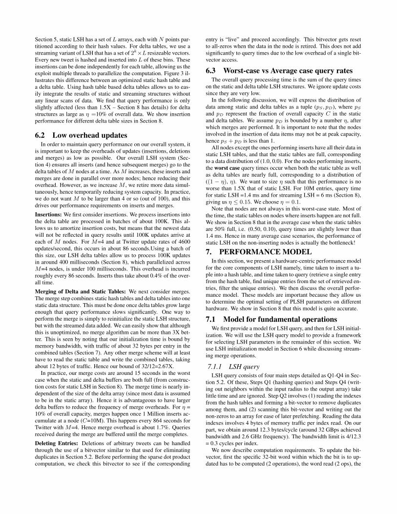
Section 5, static LSH has a set of L arrays, each withN points par-titioned according to their hash values. For delta tables, we use astreaming variant of LSH that has a set of 2k×L resizeable vectors.Every new tweet is hashed and inserted into L of these bins. Theseinsertions can be done independently for each table, allowing us theexploit multiple threads to parallelize the computation. Figure 3 il-lustrates this difference between an optimized static hash table anda delta table. Using hash table based delta tables allows us to eas-ily integrate the results of static and streaming structures withoutany linear scans of data. We find that query performance is onlyslightly affected (less than 1.5X – Section 8 has details) for deltastructures as large as η =10% of overall data. We show insertionperformance for different delta table sizes in Section 8.

6.2 Low overhead updatesIn order to maintain query performance on our overall system, it

is important to keep the overheads of updates (insertions, deletionsand merges) as low as possible. Our overall LSH system (Sec-tion 4) ensures all inserts (and hence subsequent merges) go to thedelta tables ofM nodes at a time. AsM increases, these inserts andmerges are done in parallel over more nodes; hence reducing theiroverhead. However, as we increase M , we retire more data simul-taneously, hence temporarily reducing system capacity. In practice,we do not want M to be larger than 4 or so (out of 100), and thisdrives our performance requirements on inserts and merges.

Insertions: We first consider insertions. We process insertions intothe delta table are processed in batches of about 100K. This al-lows us to amortize insertion costs, but means that the newest datawill not be reflected in query results until 100K updates arrive ateach of M nodes. For M=4 and at Twitter update rates of 4600updates/second, this occurs in about 86 seconds.Using a batch ofthis size, our LSH delta tables allow us to process 100K updatesin around 400 milliseconds (Section 8), which parallelized acrossM=4 nodes, is under 100 milliseconds. This overhead is incurredroughly every 86 seconds. Inserts thus take about 0.4% of the over-all time.

Merging of Delta and Static Tables: We next consider merges.The merge step combines static hash tables and delta tables into onestatic data structure. This must be done once delta tables grow largeenough that query performance slows significantly. One way toperform the merge is simply to reinitialize the static LSH structure,but with the streamed data added. We can easily show that althoughthis is unoptimized, no merge algorithm can be more than 3X bet-ter. This is seen by noting that our initialization time is bound bymemory bandwidth, with traffic of about 32 bytes per entry in thecombined tables (Section 7). Any other merge scheme will at leasthave to read the static table and write the combined tables, takingabout 12 bytes of traffic. Hence our bound of 32/12=2.67X.

In practice, our merge costs are around 15 seconds in the worstcase when the static and delta buffers are both full (from construc-tion costs for static LSH in Section 8). The merge time is nearly in-dependent of the size of the delta array (since most data is assumedto be in the static array). Hence it is advantageous to have largerdelta buffers to reduce the frequency of merge overheads. For η =10% of overall capacity, merges happen once 1 Million inserts ac-cumulate at a node (C=10M). This happens every 864 seconds forTwitter with M=4. Hence merge overhead is about 1.7%. Queriesreceived during the merge are buffered until the merge completes.

Deleting Entries: Deletions of arbitrary tweets can be handledthrough the use of a bitvector similar to that used for eliminatingduplicates in Section 5.2. Before performing the sparse dot productcomputation, we check this bitvector to see if the corresponding

entry is “live” and proceed accordingly. This bitvector gets resetto all-zeros when the data in the node is retired. This does not addsignificantly to query times due to the low overhead of a single bit-vector access.

6.3 Worst-case vs Average case query ratesThe overall query processing time is the sum of the query times

on the static and delta table LSH structures. We ignore update costssince they are very low.

In the following discussion, we will express the distribution ofdata among static and delta tables as a tuple (pS , pD), where pSand pD represent the fraction of overall capacity C in the staticand delta tables. We assume pD is bounded by a number η, afterwhich merges are performed. It is important to note that the nodesinvolved in the insertion of data items may not be at peak capacity,hence pS + pD is less than 1.

All nodes except the ones performing inserts have all their data instatic LSH tables, and that the static tables are full, correspondingto a data distribution of (1.0, 0.0). For the nodes performing inserts,the worst case query times occur when both the static table as wellas delta tables are nearly full, corresponding to a distribution of((1 − η), η). We want to size η such that this performance is noworse than 1.5X that of static LSH. For 10M entries, query timefor static LSH =1.4 ms and for streaming LSH = 6 ms (Section 8),giving us η ≤ 0.15. We choose η = 0.1.

Note that nodes are not always in this worst-case state. Most ofthe time, the static tables on nodes where inserts happen are not full.We show in Section 8 that in the average case when the static tablesare 50% full, i.e. (0.50, 0.10), query times are slightly lower than1.4 ms. Hence in many average case scenarios, the performance ofstatic LSH on the non-inserting nodes is actually the bottleneck!

7. PERFORMANCE MODELIn this section, we present a hardware-centric performance model

for the core components of LSH namely, time taken to insert a tu-ple into a hash table, and time taken to query (retrieve a single entryfrom the hash table, find unique entries from the set of retrieved en-tries, filter the unique entries). We then discuss the overall perfor-mance model. These models are important because they allow usto determine the optimal setting of PLSH parameters on differenthardware. We show in Section 8 that this model is quite accurate.

7.1 Model for fundamental operationsWe first provide a model for LSH query, and then for LSH initial-

ization. We will use the LSH query model to provide a frameworkfor selecting LSH parameters in the remainder of this section. Weuse LSH initialization model in Section 6 while discussing stream-ing merge operations.

7.1.1 LSH queryLSH query consists of four main steps detailed as Q1-Q4 in Sec-

tion 5.2. Of these, Steps Q1 (hashing queries) and Steps Q4 (writ-ing out neighbors within the input radius to the output array) takelittle time and are ignored. Step Q2 involves (1) reading the indexesfrom the hash tables and forming a bit-vector to remove duplicatesamong them, and (2) scanning this bit-vector and writing out thenon-zeros to an array for ease of later prefetching. Reading the dataindexes involves 4 bytes of memory traffic per index read. On ourpart, we obtain around 12.3 bytes/cycle (around 32 GBps achievedbandwidth and 2.6 GHz frequency). The bandwidth limit is 4/12.3= 0.3 cycles per index.

We now describe computation requirements. To update the bit-vector, first the specific 32-bit word within which the bit is to up-dated has to be computed (2 operations), the word read (2 ops), the

specific bit extracted (shift & logical and - 2 ops), checked with 0(2 op) and then if it is zero, set the bit (2 ops). Further, there is aloop overhead of about 3 operations, leading to a total average ofaround 11 ops per index. Performing about 1 operation per cycle,this takes 11 cycles per index. With 8 cores, this goes down to 11/8= 1.4 cycles per index. Further, scanning the bit-vector consumesabout 10 ops per 32-bits of the bit-vector to load, scan and write thedata, and another 4 ops for loop overheads. Hence this takes about14/8 = 1.75 cycles per 32-bits of N , or 0.6M cycles for N=10M.This is independent of number of indexes read. Thus Step Q2 re-quires a total of TQ2 = 1.4 cycles/duplicated index + 0.6M cycles,and is compute bound.

Step Q3 requires the reading of the tweet data for the specificdata items to be compared to the tweet. This is only required forthe unique indexes obtained in Step Q2. However, each data itemread involves high bandwidth consumption of around 4 cache linesor about 256 bytes. To understand this, consider that transfers be-tween the memory and processor caches are done in units of cachelines (or 64 bytes), where entire lines are brought into cache even ifonly part of it is accessed. In our case, there are three data structuresaccessed (CRS format [17]). Of these, two data loads for a giventweet are typically only 30 bytes (half a cache line). However, theyare not aligned at cache line boundaries. In case the start address isin the last 30 bytes of the 64 bytes, then the access crosses a cacheline – requiring 2 caches line reads. On average, each of the ar-rays requires 1.5 cache lines read, hence a total of 4 along with thecache line from the third array. These 256 bytes of read result in256/12.3 = 20.8 cycles per data item accessed. Hence TQ3 = 21.8cycles/unique index (or call to sparse dot product).

7.1.2 LSH initializationLSH initialization involves two main steps - hashing the input

data and insertion into the hash tables. As per Section 5.1, hashingis compute intensive, and performs operations for each non-zeroelement. The total cost is equal to N*NNZ, where the averagenumber of non-zeros NNZ ∼ 7.2 for Twitter data. For each suchelement, steps H1 and H2 are performed with each of the m*k/2hash values for that dimension. Each such operation involves loadof the hash (2 ops), multiply (1 ops), load output value (2 ops), addto output (1 op), store output (2 ops). In addition, about 3 opera-tions are required for handling looping. Thus a total of 11 ops foreach hash and non-zero data item combination. These operationsparallelize well (11/8 ops in parallel), and also vectorize well (closeto 8X speedup using AVX), resulting in (11/8/8) ops/hash/non-zerodata. For k=16 and m=40, and assuming one cycle per operation,hashing takes a total of TH = 412 cycles/tweet.

Insertion into the hash table itself involves three steps - StepsI1-I3 (Section 5.1). Step I1 involves reading of each hash twice (8bytes), reading the data index (4 bytes), writing out the rearrangeddata indexes (4 bytes) and writing the offsets (4 bytes). Each writealso involves a read for cache coherence, hence total memory trafficof 8 + 4*2 + 4*2 = 24 bytes per data item per first-level hash ta-ble. This phase is bandwidth limited, with a performance of TI1 =24/12.3 = 1.96 cycles * m = 1.96m cycles/tweet. With m=40, thisis around 78 cycles/tweet. Step I2 involves creating each hash usedin second-level insert. For each of the L hash tables obtained us-ing pairs of hash functions (ui, uj), computing bandwidth require-ments shows that 16 bytes of traffic is required. Step I3 performssecond level insertions into the L hash tables, and takes another16 bytes traffic per table. For m=40, L=780, hence TI2 = TI3 =16*780 /12.3 = 1015 cycles/tweet. Hence total insertion time isTI = TI1 + TI2 + TI3 = 2108 cycles/tweet.

Total construction takes TH + TI = 2520 cycles/tweet. More

than 80% of the time is spent in steps TI2 and TI3, which are band-width limited with about 32 bytes of traffic per tweet per hash table.Section 8 shows that this is fast enough to use in streaming merge.

7.2 Overall PLSH performance modelHere, we put things together with the overall LSH algorithm pa-

rameters such as (number of entries expected to be retrieved fromthe hash tables, number of unique entries) to give the overall model.This uses the k, L (or m),R parameters together with the funda-mental operation times above.

We describe how to select the parameters required by the LSHalgorithm. First, we set the failure probability δ (i.e., the probabilityof not reporting a particular near neighbor) to 10%. This guaranteesthat a vast majority (90%) of near neighbors are correctly reported.As seen in Section 8, this is a conservative estimate - in reality thealgorithm reports 92% percent of the near neighbors.

Second, we choose the radius R. Its value is tailored to the par-ticular data set, to ensure that the points within the angular distanceR are indeed ”similar”. We have determined empirically that forthe Twitter data set the value R ≈ 0.9 satisfies this criterion.

Given R and δ, it remains to select the parameters k and L ofthe LSH algorithm, to ensure that eachR-near neighbor is reportedwith probability at least 1 − δ. To this end, we need to derive aformula that computes this probability for given k and L (or m).

Fast LSH Consider a query point q and a data point v. Let t bethe distance between q and v, and p = p(t). We need to derive anexpression for the probability that the algorithm reports a point thatis within the distance R from the query point. With functions gi,the point is not retrieved if q and v collide on only zero or one ofthe functions ui. The probability of the latter event is equal to

P ′(t, k,m) = 1−(

1− p(t)k/2)m−m·p(t)k/2·

(1− p(t)k/2

)m−1

The algorithm chooses k and m such that P ′(R, k,m) ≥ 1− δ.

7.3 Parameter selectionThe values of k, L are chosen as a function of the data set to

minimize the running time of a query while ensuring that each R-near neighbor is reported with probability 1 − δ. Specifically, weenumerate pairs (k,m) such that P ′(R, k,m) ≥ 1 − δ, and foreach of the pair we estimate the total running time.

We decompose the running time of the query into 4 componentsas mentioned in Section 5.2. Of the 4 steps, steps Q2 and Q3 dom-inate the runtime, so we focus on those components only. StepQ2 concatenates the indices of the points found in all L buckets,and determines the unique data indexes. This takes time TQ2 ·#collisions, where #collisions is the number of collisions of pointsand queries in all of the L buckets. Note that a point found in mul-tiple buckets is counted multiple times.

The expected value of #collisions for query q is

E[#collisions] = L ·∑v∈P

pk(distance(q, v)) (7.1)

Step Q3 uses the unique indices to look up the full data table,and computes the actual distance between the query and the dataitem. This takes time TQ3 · #unique where #unique is the numberof unique indices found. The expected value of #unique for q is

E[#unique] =∑v∈P

P ′(distance(q, v), k, L) (7.2)

In summary, the parameters k andm (and thereforeL = m(m−1)/2) are selected such that the expression

TQ2E[#collisions] + TQ3E[#unique]

is minimized, subject to

P ′(R, k,m) ≥ 1− δ (7.3)

(L ·N + 2k · L) ∗ 4 ≤ Memory in bytes (7.4)

This can be done by enumerating k = 1, 2, . . . kmax, and foreach k selecting the smallest value of m satisfying Equation 7.3.The values ofE[#unique] andE[#collisions] can be estimated froma given dataset using equations 7.1 and 7.2 through sampling. Weuse a random set of 1000 queries and 1000 data points for generat-ing these estimates.

For small amounts of data, we can set kmax to 40, as for largerk the collision probability for two points within distance R wouldbe less than p(t)k = 0.7140 ≤ 10−6. For large amounts of data,kmax is determined by the amount of RAM in the system. Thestorage required for the hash tables increases with L, which in turnincreases super-linearly with k. The L · N term in Equations 7.4dominates memory requirements. For 10 million points in a ma-chine with 64GB of main memory, we can only store 1600 hashtables (excluding other data structures). Typically, we want to storeabout 1000 hash tables. This fixes the maximum value of m to be44 and the largest k to satisfy Equation 7.3 then is 16. Enumerationcan proceed as earlier and the best value of (k,m) is chosen.

8. EVALUATIONWe now evaluate the performance of our algorithm on an Intel®

Xeon® processor E5-2670 based system with 8 cores running at 2.6GHz. Each core has a 64 KB L1 cache and a 256 KB L2 cache, andsupports 2-way Simultaneous Multi-Threading (SMT). All coresshare a 20MB last level cache. Bandwidth to main memory is 32GB/s. Our system has 64 GB memory on each node and runs RHEL6.1. We use the Intel® Composer XE 2013 compiler for compilingour code1. Our cluster has 100 nodes connected through Infiniband(IB) and Gigabit Ethernet (GigE). All our multi node experimentsuse MPI to communicate over IB.Benchmarks and Performance Evaluation: We run PLSH on1.05 billion tweets collected from September 2012 to February 2013.These tweets were cleaned by removing non-alphabet characters,duplicates and stop words. Each tweet is encoded as a sparse vec-tor in a 500,000-dimensional space corresponding to the size of thevocabulary used. In order to give more importance to less commonwords, we use an Inverse Document Frequency (IDF) score thatgives greater weight to less frequently occurring words. Finally wenormalize each tweet vector to transform it into a unit vector. Forsingle node experiments, we use about 10.5 million tweets. The op-timal LSH parameters were selected using our performance model.We use the following parameters: k = 16,m = 40, L = 780, D =500, 000, R = 0.9, δ = 0.1.

For queries, we use a random subset of 1000 tweets from thedatabase. 0-length queries are possible if the tweet is entirely com-posed of special characters, unicode characters, numerals, wordsthat are not part of the vocabulary etc. Since these queries willnot find any meaningful matches, we ignore these queries. Eventhough we use a random subset of the input data for querying, wehave found empirically that queries generated from user-given textsnippets perform equally well.

8.1 PLSH vs exact algorithms1

Intel’s compilers may or may not optimize to the same degree for non-Intel microprocessors for optimizations that arenot unique to Intel microprocessors. These optimizations include SSE2, SSE3, and SSE3 instruction sets and other opti-mizations. Intel does not guarantee the availability, functionality, or effectiveness of any optimization on microprocessorsnot manufactured by Intel. Microprocessor-dependent optimizations in this product are intended for use with Intel micro-processors. Certain optimizations not specific to Intel microarchitecture are reserved for Intel microprocessors. Pleaserefer to the applicable product User and Reference Guides for more information regarding the specific instruction setscovered by this notice. Notice revision #20110804

Algorithm # distance computations Runtime

Exhaustive search 10,579,994 115.35 msInverted index 847,027.9 > 21.81 ms

PLSH 120,345.7 1.42 ms

Table 2: Runtime comparison between PLSH and other deterministicnearest neighbor algorithms. Inverted index excludes time to generatecandidate matches, only including the time for distance computations.

In order to prove empirically that PLSH does indeed performsignificantly better than other algorithms, we perform a compari-son against an exhaustive search and one based on an inverted in-dex. The exhaustive search algorithm calculates the distance from aquery point to all the points in the input data and reports only thosepoints that lie within a distance R from the query. An inverted in-dex is a data structure that works by finding a set of documents thatcontain a particular word. Given a query text, the inverted indexis used to get the set of all documents (tweets) that contain at leastone of the words in the document. These candidate points are fil-tered using the distance criterion. Both the exhaustive search andinverted index are deterministic algorithms. LSH, in contrast, is arandomized algorithm with a high probability of finding neighbors.

Table 2 gives the average number of distance computations thatneed to be performed for each of the above mentioned algorithmsfor a query (averaged from a set of 1000 queries) and their runtimeson 10.5 million tweets on a single node. Since we expect that allthese runtimes are dominated by the data lookups involved in dis-tance computations, it is clear that PLSH performs much better thanboth these techniques. For inverted index, we do not include thetime to generate the candidate matches (this would involve lookupsinto the inverted index structure), whereas for PLSH we include alltimes (hash table lookups and distance calculations). Even assum-ing lower bounds for inverted index, PLSH is about 15× faster thaninverted index and 81× faster than exhaustive search while achiev-ing 92% accuracy. Note that all algorithms have been parallelizedto use multiple cores to execute queries.

8.2 Effect of optimizationsWe now show the breakdown of different optimizations performed

for improving the performance of LSH as described in Section 5.Figure 4 shows the effect of the performance optimizations appliedto the creation (initialization) of LSH, as described in Section 5.1.The unoptimized version performs hash table creation using a sep-arate k-bit key for each of the L tables. Starting from an unop-timized implementation (1-level partitioning), we achieve a 3.7×improvement through the use of our new 2-level hash table and op-timized PLSH algorithm, as well as use of shared hash tables andcode vectorization. All the versions are parallelized on 16 threads.

Figure 5 provides a breakdown of the effects of the optimizationson LSH query performance described in Section 5.2. The series ofoptimizations applied to the unoptimized implementation includethe usage of bitvector for removing duplicate candidates, optimiz-ing the sparse dot product calculation, enabling prefetching of dataand the usage of large pages to avoid TLB misses. The unopti-mized implementation uses the C++ STL set to remove duplicatesand uses the unoptimized sparse dot calculation (Section 5.2.3).Compared to this, our final version gives a speedup of 8.3×.

8.3 Performance Model ValidationIn this section, we show that the performance model proposed

in Section 7 corresponds closely to the real world performance ofPLSH creation and querying. Figure 6 compares the estimated andreal runtimes of PLSH. Some of the error comes from the estimatesof E[#collisions] and E[#unique] through sampling and other er-rors from inaccurately modeling the PLSH component kernels. We

20000

30000

40000

50000

60000

70000

e in

milliseconds

0

10000

20000

No optimizations +2 level hashtable +shared tables +vectorization

Tim

Figure 4: PLSH creation performance breakdown. The optimizationsare described in Section 5.

4000

6000

8000

10000

12000

me in

milliseconds

0

2000

No optimizations

+bitvector +optimized sparse DP

+sw prefetch +large pages

Tim

Figure 5: PLSH query performance breakdown (for 1000 queries).The optimizations are described in Section 5.

demonstrate the performance model accuracy on an additional textdataset obtained from 8 million Wikipedia article abstracts with a500K vocabulary. We find that the error margin is less than 15% forboth PLSH creation and querying on Twitter data and less than 25%for the Wikipedia data. Even more importantly, we can accuratelyestimate relative performance changes correctly when parameterschange. Figure 7 demonstrates that our performance model can beused for tuning LSH parameters (for R = 0.9, δ = 0.1 ). As men-tioned earlier, given a main memory Twitter and Wikipedia datarespectively. In all cases, our model provides reliable estimates ofboth relative and absolute performance numbers. These results sug-gest that our model can be used both to estimate whether a givenhardware configuration can manage a particular query/insert loadand also to optimize parameter selection.

Estimated

Actual

LSH Query

Search (Step Q3)

Bitvector (Step Q2)

0 500 1000 1500 2000

Estimated

Time in milliseconds

(Step Q2)

Estimated

Actual

LSH Creation

Hashing

Step I1

Step I2

0 5000 10000 15000 20000

Estimated

Time in milliseconds

Step I3

Figure 6: Estimated vs actual runtimes for PLSH creation & querying(1000 queries).

8.4 ScalingIn this section, we discuss the scaling performance of PLSH.

First, Figure 8 shows how the performance of PLSH improves on asingle 8-core node with increasing number of threads. We see thatwe achieve a speedup of 7.2× for PLSH initialization and 7.8× forquerying.These performance numbers have already been shown tobe very close to the achievable bandwidth and compute limits ofthe hardware.

Figure 9 shows the performance of PLSH as we add more dataand nodes to our problem. Here, we keep the amount of work perprocessor constant and increase the number of processors (and cor-respondingly, the amount of data). This demonstrates that our im-plementation is indeed scalable to more than a billion tweets with-out any load balancing or communication problems. We define loadbalance as the ratio of the maximum to average runtime. Results in-dicate that this ratio is smaller than 1.3 (ideal is 1.0) for both PLSHcreation and querying even at the largest scale. We also found that

15002000250030003500400045005000

e in

milliseconds

Estimated Query runtime (Twitter)Actual Query runtime (Twitter)Estimated Query runtime (Wikipedia)Actual Query runtime (Wikipedia)

0500

10001500

(12, 21) (14, 29) (16, 40) (18, 55)

Tim

PLSH parameters (k,m)

Figure 7: Estimated vs actual runtimes for varying k and m (1000 queries)

20000

40000

60000

80000

100000

120000

me in

milliseconds

Initialization timeQuery time

0

20000

1 2 4 8 16 (SMT)

Tim

Number of threads

Figure 8: Scaling performance with increasing threads on a single node.

the query communication time is less than 20 ms in all cases (lessthan 1% of overall runtime).

5000

10000

15000

20000

me in

milliseconds

Initialization (max)Initialization (min)

Initialization (avg)

Query (max)

0

5000

1 2 4 8 16 32 64 100

Tim

Number of nodes

Query (min)

Query (avg)

Figure 9: Scaling performance on multiple nodes. The data per node isfixed at 10.5 million tweets, so flat lines indicate perfect scaling.8.5 Latency vs Throughput

So far in this section, we have measured query performance on aset of 1000 queries. We do this for 2 reasons. (1) We believe thatwhile performance for an isolated query is important, most analyt-ics workloads would need to support multiple queries at the sametime. Techniques like flu tracking using Twitter [29] rely on de-tecting several concepts i.e. searching for several terms/concepts.(2) Using multithreading to process multiple queries works well inpractice compared to multithreading a single query search. Tightsynchronization is needed for processing a single query whereasmultiple independent queries can be processed simultaneously with-out the need for synchronization or locks.

Figure 10 shows the latency-vs-throughput behavior as we in-crease the number of queries processed at a time. We see that aswe increase the number of queries processed simultaneously, there

is an increase in both latency and throughput before the throughputstabilizes around 700 queries/second with about 30 queries. Thethroughput is relatively unaffected after this point.

200

300

400

500

600

700

800

ughput in queries/s

0

100

200

0 500 1000 1500

Throu

Latency in ms

Figure 10: Latency Vs Throughput for processing queries in LSH. The sizeof the query set is varied from 10 to 1000 in steps of 10.8.6 Streaming

As mentioned in Section 6, twitter is highly dynamic with about400 million tweets added per day. We need to ensure that queryperformance does not drop below 1.5X of static queries, while stillallowing for dynamic insertions. Our system achieves this.

Figure 11 shows the query performance of the system runningon a single node. The overall capacity C of the node is 10.5 mil-lion tweets. The maximum size of the delta table structure (η) is10% of the total capacity - around 1 million. The two lines in thegraph represent query behavior under different amounts of data inthe static tables. With about 50% of the overall capacity in the staticstructure, we achieve no performance degradation at all comparedto fully static tables at capacity. With 90% of the capacity in thestatic structure, we encounter query runtimes going up to 1.3× thatof 100% static tables in the worst case. Under average conditions,our streaming implementation will perform with no penalties.

0

500

1000

1500

2000

0 20 40 60 80 100

Time in

milliseconds

% data in streaming LSH (Max streaming capacity=1M)

Query time (50% static capacity)

Query time (90% static capacity)

100% Static LSH query performance

Figure 11: Streaming performance for 1000 queries with a constant amountof data in static table while data is added to the streaming tables. The dottedline represents the performance of 100% static LSH. Even in the worst case,the performance does not drop below 1.5X of static performance.

Insertion into the streaming LSH tables happens in chunks of100k tweets. Each such insertion takes about 400 ms. We mergethe streaming tables with the static tables when the streaming ta-bles reach their capacity of 1 million tweets. This merge takes 15seconds in the worst case (when static LSH is almost full). Hence,processing 1 million streaming tweets takes 19 seconds. Given thestreaming rate of 400 million tweets/day and 4 nodes to handle thestreaming data, the insert/merge processing takes a total of about30 minutes in 24 hours. In other words, about 2% of the time isspent inserting and merging data.

9. DISCUSSION AND CONCLUSIONIn this paper, we presented PLSH, a system to handle nearest

neighbor queries on large amounts of text data based on an effi-cient parallel LSH implementation. PLSH is an in-memory, mul-tithreaded distributed system capable of handling large amounts ofstreaming data while delivering very high query performance. Wedemonstrate its capabilities by running nearest neighbor queries

on a billion tweet dataset on 100 nodes in 1–2.5 ms (per query),while streaming 100’s of millions of tweets per day. We introducedseveral optimizations and a new variant that improves the time tobuild LSH tables by a factor of 3.7× and reduce query time by afactor of 8.3×. To the best of our knowledge, this makes PLSHthe fastest LSH implementation currently available. We also intro-duced a performance model that is able to predict the performanceof our implementation to within 15−25%, showing we are close toarchitectural limits and helping us pick the best PLSH parameters.ACKNOWLEDGEMENTSThis work was supported by a grant from Intel, as a part of the IntelScience and Technology Center in Big Data (ISTC-BD).10. REFERENCES[1] E2LSH. http://www.mit.edu/˜andoni/LSH/.[2] LikeLike. http://code.google.com/p/likelike/.[3] LSH-Hadoop. https://github.com/LanceNorskog/LSH-Hadoop.[4] LSHKIT. http://lshkit.sourceforge.net.[5] OptimalLSH. https://github.com/yahoo/Optimal-LSH.[6] Twitter breaks 400 million tweet-per-day barrier, sees increasing mobile

revenue. http://bit.ly/MmXObG.[7] A. Andoni and P. Indyk. Efficient algorithms for substring near neighbor

problem. In Proceedings of SODA, pages 1203–1212, 2006.[8] A. Andoni and P. Indyk. Near-optimal hashing algorithms for approximate

nearest neighbor in high dimensions. CACM, 58, 2008.[9] N. Askitis and J. Zobel. Cache-conscious collision resolution in string hash

tables. In SPIRE, pages 92–104, 2005.[10] B. Bahmani, A. Goel, and R. Shinde. Efficient distributed locality sensitive

hashing. In CIKM, pages 2174–2178. ACM, 2012.[11] J. L. Bentley. Multidimensional binary search trees used for associative

searching. CACM, 18(9):509–517, 1975.[12] C. Bohm, S. Berchtold, and D. A. Keim. Searching in high-dimensional spaces:

Index structures for improving the performance of multimedia databases. ACMComputing Surveys, 33(3):322–373, Sept. 2001.

[13] M. Charikar. Similarity estimation techniques from rounding. In Proceedings ofSTOC, pages 380–388, 2002.

[14] L. Chen, M. T. Ozsu, and V. Oria. Robust and fast similarity search for movingobject trajectories. In Proceedings of SIGMOD, 2005.

[15] A. S. Das, M. Datar, A. Garg, and S. Rajaram. Google news personalization:scalable online collaborative filtering. In WWW, 2007.

[16] A. Dasgupta, R. Kumar, and T. Sarlos. Fast locality-sensitive hashing. InSIGKDD, pages 1073–1081. ACM, 2011.

[17] I. S. Duff, A. M. Erisman, and J. K. Reid. Direct methods for sparse matrices.Oxford University Press, Inc., 1986.

[18] P. C.-M. K. A. P. Haghani. Lsh at large – distributed knn search in highdimensions. In WebDB, 2008.

[19] M. Henzinger. Finding near-duplicate web pages: a large-scale evaluation ofalgorithms. In SIGIR, 2006.

[20] P. Indyk and R. Motwani. Approximate nearest neighbor: towards removing thecurse of dimensionality. In Proceedings of STOC, 1998.

[21] C. Kim, E. Sedlar, J. Chhugani, T. Kaldewey, et al. Sort vs. hash revisited: Fastjoin implementation on multi-core cpus. PVLDB, 2(2):1378–1389, 2009.

[22] T. J. Lehman and M. J. Carey. A study of index structures for main memorydatabase management systems. In VLDB, 1986.

[23] Y. Li, J. M. Patel, and A. Terrell. Wham: A high-throughput sequencealignment method. TODS, 37(4):28:1–28:39, Dec. 2012.

[24] F. Liu, C. Yu, W. Meng, and A. Chowdhury. Effective keyword search inrelational databases. In Proceedings of ACM SIGMOD, 2006.

[25] G. S. Manku, A. Jain, and A. Das Sarma. Detecting near-duplicates for webcrawling. In Proceedings of WWW, 2007.

[26] E. Mohr, D. A. Kranz, and R. H. Halstead. Lazy task creation: a technique forincreasing the granularity of parallel programs. IEEE Transactions on Paralleland Distributed Systems, 2:185–197, 1991.

[27] J. Pan and D. Manocha. Fast GPU-based locality sensitive hashing for k-nearestneighbor computation. In SIGSPATIAL, 2011.

[28] S. Petrovic, M. Osborne, and V. Lavrenko. Streaming first story detection withapplication to twitter. In NAACL, volume 10, pages 181–189, 2010.

[29] A. Sadilek and H. Kautz. Modeling the impact of lifestyle on health at scale. InProceedings of ACM ICWSDM, pages 637–646, 2013.

[30] N. Satish, C. Kim, J. Chhugani, et al. Fast sort on CPUs and GPUs: a case forbandwidth oblivious SIMD sort. In SIGMOD, 2010.

[31] M. Slaney, Y. Lifshits, and J. He. Optimal parameters for locality-sensitivehashing. Proceedings of the IEEE, 100(9):2604–2623, 2012.

[32] X. Yan, P. S. Yu, and J. Han. Substructure similarity search in graph databases.In Proceedings of SIGMOD, 2005.