Streaming Multigrid for Gradient-Domain Operations on Large Images

Michael Kazhdan

Johns Hopkins University

Hugues Hoppe

Microsoft Research

Abstract

We introduce a new tool to solve the large linear systems arisingfrom gradient-domain image processing. Specifically, we developa streaming multigrid solver, which needs just two sequential passesover out-of-core data. This fast solution is enabled by a combina-tion of three techniques: (1) use of second-order finite elements(rather than traditional finite differences) to reach sufficient accu-racy in a single V-cycle, (2) temporally blocked relaxation, and(3) multi-level streaming to pipeline the restriction and prolonga-tion phases into single streaming passes. A key contribution isthe extension of the B-spline finite-element method to be compati-ble with the forward-difference gradient representation commonlyused with images. Our streaming solver is also efficient for in-memory images, due to its fast convergence and excellent cachebehavior. Remarkably, it can outperform spatially adaptive solversthat exploit application-specific knowledge. We demonstrate seam-less stitching and tone-mapping of gigapixel images in about anhour on a notebook PC.

Keywords: out-of-core multigrid solver, B-spline finite elements,Poisson equation, gigapixel images, multi-level streaming.

1 Introduction

Many recent image processing techniques operate in the gradientdomain. They extract gradient fields from one or more images, pro-cess the data to construct a desired gradient field, and solve for anew image whose pixel differences best fit the desired gradients.

For example, lighting is removed from an image by zeroing smallgradients [Horn 1974], or by selecting the median of gradients frommultiple exposures [Weiss 2001]. A high dynamic range (HDR) im-age is tone-mapped by adaptively attenuating luminance gradients[Fattal et al. 2002]. Overlapping images are stitched seamlessly bymerging their gradients [Perez et al. 2003; Agarwala et al. 2004;Levin et al. 2004]. Shadows are removed by zeroing large lumi-nance gradients in regions of constant chromaticity [Finlayson et al.2002]. Undesirable reflections are removed in flash and ambientimage pairs [Agrawal et al. 2005]. Photographic tone managementis improved using gradient constraints [Bae et al. 2006]. Novelpainterly effects are possible with interactive gradient-domain mod-eling [McCann and Pollard 2008]. In all these applications, the finalimage is recovered from the processed gradient by solving a Pois-son equation, which is discretized to form a sparse linear system.

Recent work has begun to address the processing of large (e.g.gigapixel) images [Kopf et al. 2007b]. In this case the resultinglinear systems, and often the images themselves, are too large tofit in main memory. Consequently, direct solution techniques likeCholesky factorization become impractical, and traditional relax-ation techniques like conjugate gradients and multigrid are ineffi-

cient because they require many iterations over out-of-core data. Asreviewed in Section 2, the associated Poisson problem can be madetractable for some specific applications through adaptive discretiza-tion, and has also been addressed using heuristic approximations.

Our contribution We introduce a general, efficient, accuratesolver for Poisson equations over large images. We combine multi-grid computation with a data streaming framework, to allow out-of-core processing on gigapixel images. Our scheme maintains smallmoving windows of data in memory (and cache) by sequentiallyadvancing through the out-of-core data. Because the solver com-putation outpaces disk I/O, the speed bottleneck is the number ofstreaming passes through the image data. We are able to obtain suf-ficient accuracy in just 2 passes, even on gigapixel images. Threekey components enable this efficient solution:

• Whereas prior image solvers use finite differences, we discretizethe Poisson equation with second-order finite elements, allowingus to reach sufficiently low error in a single multigrid V-cycle.

• Within a grid level, temporally blocked relaxation evaluates sev-eral Gauss-Seidel relaxations as a single streaming operation.

• We interleave these multiresolution relaxations using multi-levelstreaming so that the restriction and prolongation phases of a V-cycle can each be pipelined into a single streaming pass.

Compared to finite differences, second-order finite elements requirelarger stencils for relaxation, restriction, and prolongation. Thoughthese larger stencils increase computational load, they improve thesolver convergence rate significantly. On most images, a second-order solver with a single V-cycle finds a solution with maximumerror markedly less than 1/256 of the pixel value range, i.e. wellwithin the requisite precision for 8-bit/channel images. We showthat additional V-cycles further decrease error at a steady rate, andmoreover each such cycle requires just one extra streaming pass.

Since forward-difference representations of gradient fields are com-monly used as constraints in image processing, it is essential thatour system support them. Although finite differences and finite el-ements provide alternate interpretations of image derivatives, weshow that the use of B-spline elements lets us correctly solve forimages subject to finite-difference constraints.

In this paper we consider instances of the Poisson equation withunconstrained (more precisely, Neumann) boundary conditions,which supports many gradient-domain techniques. The Poissonequation corresponds to an elliptical partial differential equationwith spatially constant coefficients. In Section 10 we discuss fu-ture extensions for more general boundary conditions or PDEs.

While our main motivation is the processing of huge images, wefind that the streaming multigrid approach is also beneficial forsmaller in-memory images due to its fast convergence and excel-lent cache behavior. On a single CPU core, we are able to solve a3-channel, 16-megapixel gradient-domain problem with an rms er-ror on the order of 10−5 in 15 seconds. The ongoing transition tomany-core architectures will likely favor methods with a high ratioof local computation to memory bandwidth. In effect, memory ac-cess may become the next I/O bottleneck. Because our streamingscheme offers many opportunities for computational parallelism onlocal data, with few accesses to global memory, it is well suited forfuture scalability.

2 Related work

Due to the numerous applications of the Poisson equation, manysolution techniques have been explored. The fast Fourier transformis an elegant scheme, but has O(n logn) time complexity. A di-rect solution can also be obtained by sparse matrix factorization,but the resulting factors may require significant temporary mem-ory. Iterative solvers like Gauss-Seidel and conjugate gradients arememory-efficient but usually require many iterations over the data.The number of iterations can be reduced using either multiresolu-tion preconditioners [Gortler and Cohen 1995; Szeliski 2006] ormultigrid solvers [Brandt 1977; Briggs et al. 2000]. Such tech-niques have also been implemented efficiently on the GPU [Bolzet al. 2003; Goodnight et al. 2003; Goddeke et al. 2008].

Most previous work has focused on Poisson systems that fit inmemory. Toledo [1999] presents an excellent survey of out-of-corealgorithms for large linear systems. Most algorithms assume thatwhile the system matrix may be stored on disk, the solution vectoritself (i.e. the image in our case) still fits in memory. In general, itwas previously thought that advanced iterative techniques, includ-ing multigrid, are difficult to schedule out-of-core.

One approach for out-of-core images is to solve the problem ona coarser-resolution grid and then upsample the resulting approx-imation [Kopf et al. 2007a]. However, maintaining sharp featuresinvolves heuristics that may not always be robust.

In some cases where the solution is known to have low frequencyalmost everywhere, the problem size can be reduced by adaptivelypartitioning the domain. For image stitching, Agarwala [2007] ex-ploits the fact that if an initial guess is generated by copying pixelsfrom the input images, the residual has low frequency away fromthe image seams and the Poisson equation can be solved over aquadtree adapted to the seams. Such adaptive partitions have alsobeen used to solve the Poisson equation in the context of fluidflow simulation [Losasso et al. 2004] and surface reconstruction[Kazhdan et al. 2006].

Our method addresses the general case where (1) the Poisson equa-tion must be solved accurately everywhere, (2) the problem sizecannot be reduced, and (3) no initial solution guess is available.

Bolitho et al. [2007] introduce multi-level streaming for an out-of-core Poisson solution. Their method, which implements a cascadic(prolongation-only) solver, has adequate accuracy for surface re-construction but not for image processing. In this work, we showthat the multi-level streaming idea can be integrated into a finite-element multigrid solver that performs multiple Gauss-Seidel itera-tions at each resolution and implements a complete V-cycle in onlytwo streaming passes. We demonstrate that the resulting solution isaccurate enough for gradient-domain image processing.

3 Gradient-domain problem as Poisson solution

In the continuous setting, we seek an image U(x,y) on a domain

Ω = [0,1]2 whose gradient is closest to a desired gradient field~G(x,y), i.e. to find U minimizing ‖∇U − ~G‖. Using the normalequation, this minimization is equivalent to solving the Poissonequation ∆U = F , where ∆ = ∇ ·∇ is the Laplacian operator and

F = ∇ · ~G is the divergence of the desired gradient.

Of course, an image is typically represented by a discrete N ×Ngrid u of pixel values ui, j . One of the challenges in setting upthe Poisson equation in the context of image processing is that thePoisson equation is a continuous beast requiring the computationof derivatives while images are inherently discrete. There are twoways to address this. The first is to discretize derivatives, resulting

in the traditional finite-difference approach, often used in imageprocessing (Section 4). The second is to treat images as continu-ous functions, resulting in the finite-element approach pursued here(Section 5).

4 Review of finite-difference multigrid

Both the image gradient ∇U and desired gradient ~G are com-monly expressed as forward differences of adjacent pixels values,i.e. ∇ui, j = (ui+1, j−ui, j, ui, j+1−ui, j) and similarly for the forward

differences ~gi, j = (gxi, j,g

yi, j). With such a discretization, one seeks

to minimize ‖∇u−~g‖, which is equivalent to solving a sparse lin-ear system Lu = f . Each row of the matrix L corresponds to thefive-point Laplacian stencil with weight −4 at the current pixeland weight 1 at the four adjacent pixels. And, the Laplacian con-straint vector f has entries defined in terms of backward differencesfi, j = gx

i, j−gxi−1, j +g

yi, j−g

yi, j−1. For simplicity we use u (and sim-

ilarly f ) to denote both an N×N array of pixels ui, j and a vector

(u0 . . .uN2−1)T of the same pixels in raster order.

To avoid constraining boundary values in the Poisson equation, thedefinition of ∇u and the construction of f are modified at domainboundaries to assume trivial Neumann conditions, i.e. zero cross-boundary derivatives. The resulting matrix L does not have fullrank, since the solution is only determined up to an additive con-stant. However, a solution always exists because the constructionof f using the divergence operator guarantees compatibility.

A simple approach for solving the linear system Lu = f is to applyrepeated iterations of Gauss-Seidel relaxation. In each iteration, theimage u is updated by successively modifying each pixel ui whileholding the other pixels constant:

ui =

(

fi−∑j 6=i

Li, ju j

)

/ Li,i.

Because the Laplacian operator L has local 2D support, these relax-ation updates only require access to local data.

However, a limitation of Gauss-Seidel relaxation is that it convergesslowly on the low-frequency components of the solution. Multi-grid is introduced to overcome this [Briggs et al. 2000]. The sin-gle system Lu = f is replaced by a multiresolution set of systems

Llul = f l

, where ul ∈RN2

l with Nl = 2l . Restriction and prolon-gation linear operators are defined to transition between levels:

Rll+1 : R

N2l+1 → R

N2l and Pl+1

l : RN2

l → RN2

l+1 ,

typically using local weighted averaging and bilinear interpolation.

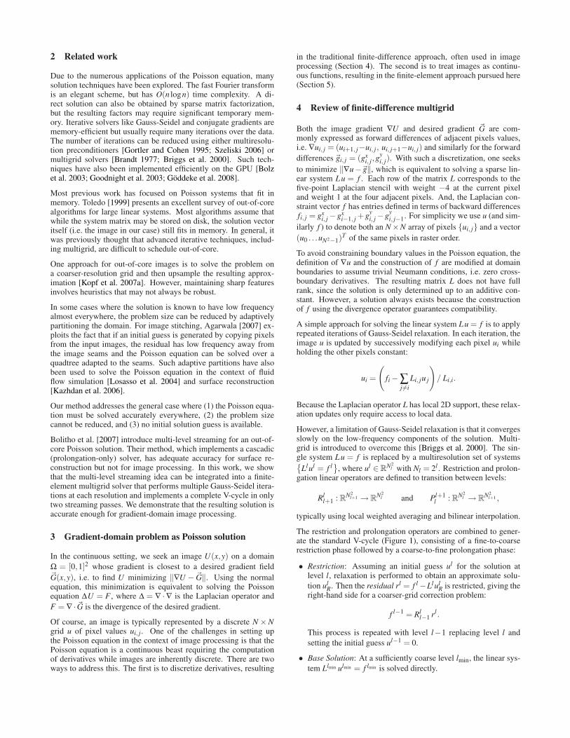
The restriction and prolongation operators are combined to gener-ate the standard V-cycle (Figure 1), consisting of a fine-to-coarserestriction phase followed by a coarse-to-fine prolongation phase:

• Restriction: Assuming an initial guess ul for the solution atlevel l, relaxation is performed to obtain an approximate solu-

tion ulR. Then the residual rl = f l−Llul

R is restricted, giving theright-hand side for a coarser-grid correction problem:

f l−1 = Rll−1 rl .

This process is repeated with level l−1 replacing level l and

setting the initial guess ul−1 = 0.

• Base Solution: At a sufficiently coarse level lmin, the linear sys-

tem Llmin ulmin = f lmin is solved directly.

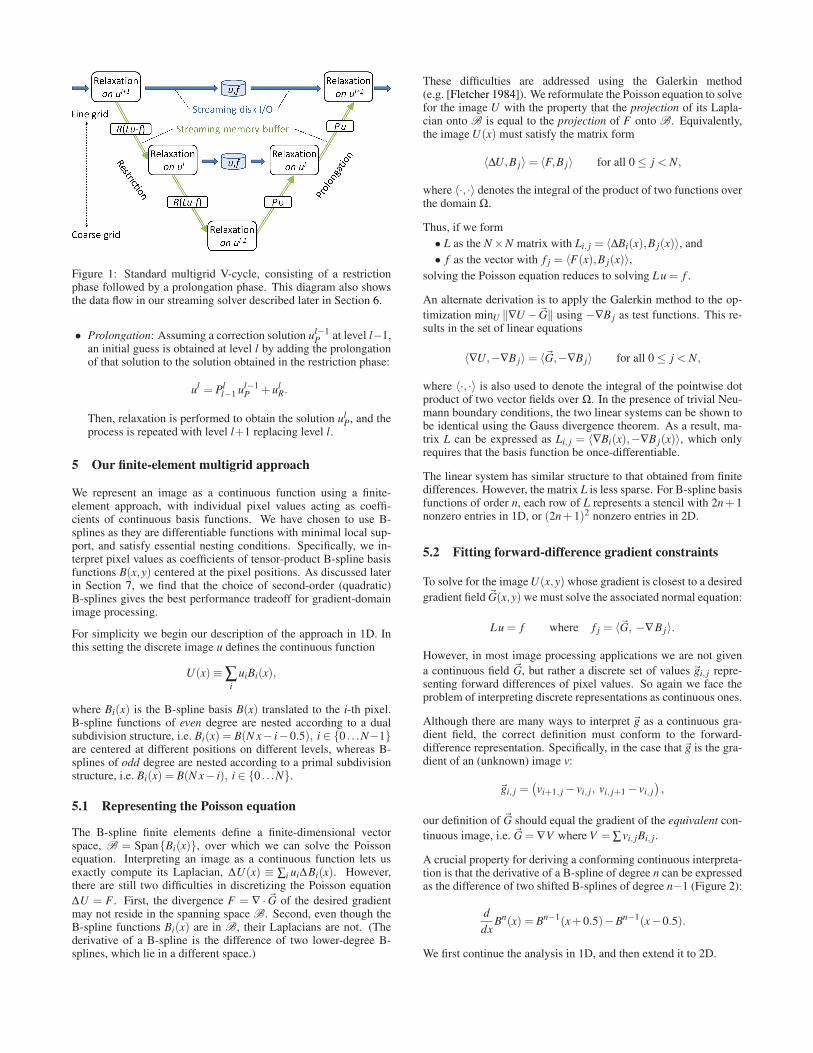
Figure 1: Standard multigrid V-cycle, consisting of a restrictionphase followed by a prolongation phase. This diagram also showsthe data flow in our streaming solver described later in Section 6.

• Prolongation: Assuming a correction solution ul−1P at level l−1,

an initial guess is obtained at level l by adding the prolongationof that solution to the solution obtained in the restriction phase:

ul = Pll−1 ul−1

P +ulR.

Then, relaxation is performed to obtain the solution ulP, and the

process is repeated with level l+1 replacing level l.

5 Our finite-element multigrid approach

We represent an image as a continuous function using a finite-element approach, with individual pixel values acting as coeffi-cients of continuous basis functions. We have chosen to use B-splines as they are differentiable functions with minimal local sup-port, and satisfy essential nesting conditions. Specifically, we in-terpret pixel values as coefficients of tensor-product B-spline basisfunctions B(x,y) centered at the pixel positions. As discussed laterin Section 7, we find that the choice of second-order (quadratic)B-splines gives the best performance tradeoff for gradient-domainimage processing.

For simplicity we begin our description of the approach in 1D. Inthis setting the discrete image u defines the continuous function

U(x)≡∑i

uiBi(x),

where Bi(x) is the B-spline basis B(x) translated to the i-th pixel.B-spline functions of even degree are nested according to a dualsubdivision structure, i.e. Bi(x) = B(N x− i−0.5), i ∈ 0 . . .N−1are centered at different positions on different levels, whereas B-splines of odd degree are nested according to a primal subdivisionstructure, i.e. Bi(x) = B(N x− i), i ∈ 0 . . .N.

5.1 Representing the Poisson equation

The B-spline finite elements define a finite-dimensional vectorspace, B = SpanBi(x), over which we can solve the Poissonequation. Interpreting an image as a continuous function lets usexactly compute its Laplacian, ∆U(x) ≡ ∑i ui∆Bi(x). However,there are still two difficulties in discretizing the Poisson equation

∆U = F . First, the divergence F = ∇ · ~G of the desired gradientmay not reside in the spanning space B. Second, even though theB-spline functions Bi(x) are in B, their Laplacians are not. (Thederivative of a B-spline is the difference of two lower-degree B-splines, which lie in a different space.)

These difficulties are addressed using the Galerkin method(e.g. [Fletcher 1984]). We reformulate the Poisson equation to solvefor the image U with the property that the projection of its Lapla-cian onto B is equal to the projection of F onto B. Equivalently,the image U(x) must satisfy the matrix form

〈∆U,B j〉= 〈F,B j〉 for all 0≤ j < N,

where 〈·, ·〉 denotes the integral of the product of two functions overthe domain Ω.

Thus, if we form

• L as the N×N matrix with Li, j = 〈∆Bi(x),B j(x)〉, and

• f as the vector with f j = 〈F(x),B j(x)〉,

solving the Poisson equation reduces to solving Lu = f .

An alternate derivation is to apply the Galerkin method to the op-

timization minU ‖∇U − ~G‖ using −∇B j as test functions. This re-sults in the set of linear equations

〈∇U,−∇B j〉= 〈~G,−∇B j〉 for all 0≤ j < N,

where 〈·, ·〉 is also used to denote the integral of the pointwise dotproduct of two vector fields over Ω. In the presence of trivial Neu-mann boundary conditions, the two linear systems can be shown tobe identical using the Gauss divergence theorem. As a result, ma-trix L can be expressed as Li, j = 〈∇Bi(x),−∇B j(x)〉, which onlyrequires that the basis function be once-differentiable.

The linear system has similar structure to that obtained from finitedifferences. However, the matrix L is less sparse. For B-spline basisfunctions of order n, each row of L represents a stencil with 2n+1nonzero entries in 1D, or (2n+1)2 nonzero entries in 2D.

5.2 Fitting forward-difference gradient constraints

To solve for the image U(x,y) whose gradient is closest to a desired

gradient field ~G(x,y) we must solve the associated normal equation:

Lu = f where f j = 〈~G, −∇B j〉.

However, in most image processing applications we are not given

a continuous field ~G, but rather a discrete set of values ~gi, j repre-senting forward differences of pixel values. So again we face theproblem of interpreting discrete representations as continuous ones.

Although there are many ways to interpret ~g as a continuous gra-dient field, the correct definition must conform to the forward-difference representation. Specifically, in the case that ~g is the gra-dient of an (unknown) image v:

~gi, j =(

vi+1, j− vi, j, vi, j+1− vi, j

)

,

our definition of ~G should equal the gradient of the equivalent con-

tinuous image, i.e. ~G = ∇V where V = ∑vi, jBi, j .

A crucial property for deriving a conforming continuous interpreta-tion is that the derivative of a B-spline of degree n can be expressedas the difference of two shifted B-splines of degree n−1 (Figure 2):

d

dxBn(x) = Bn−1(x+0.5)−Bn−1(x−0.5).

We first continue the analysis in 1D, and then extend it to 2D.

Figure 2: Given a B-spline of degree n (blue), its derivative (red)can be expressed as the difference of two offset B-splines of degreen−1 (dashed green), as shown here for n=1,2.

1D case Recall that the discrete signal v expresses a continuousfunction in terms of quadratic B-splines: V (x) = ∑i vi B2

i (x), where

B2i (x) is centered in the middle of the i-th lattice cell.

To compute the derivative of V we observe that:

∇V (x) = N ·∑i

(

B1i (x)−B1

i+1(x))

vi

= N ·∑i

B1i+1(x)(vi+1− vi) = N ·∑

i

B1i+1(x)gi.

Thus, even though we are not given the original image V , we cancompute its derivative from the forward-difference representationby interpreting the values gi as coefficients of first-order B-splines.

Using this interpretation, we can directly compute the Laplacianconstraints on the right-hand side:

f j =⟨

∇V (x), −∇B2j(x)⟩

=−N ·∑i

gi

⟨

B1i+1(x),

d

dxB2

j(x)

⟩

.

2D case Recall that in the 2D case, the discrete array v defines acontinuous function using tensor products of quadratic B-splines:V (x,y) = ∑i, j vi, j B2

i (x)B2j(y). As above, we obtain

∇V (x,y) = N ·

(

∑i, j

B1i+1(x)B2

j(y)gxi, j, ∑

i, j

B2i (x)B1

j+1(y)gyi, j

)

.

And again, even though we are not given the original image V , wecan compute its gradient from the forward-difference representa-tion by interpreting the values ~gi, j as coefficients of mixed tensorproducts of first- and second-order B-splines.

Using this interpretation, we can directly compute the Laplacianconstraints on the right hand side:

fi, j = − N ·∑s,t

gxs,t

⟨

B1s+1(x),

d

dxB2

i (x)

⟩

⟨

B2t (y), B2

j(y)⟩

− N ·∑s,t

gys,t

⟨

B2s (x), B2

i (x)⟩

⟨

B1t+1(y),

d

dyB2

j(y)

⟩

.

Note that the inner products defining the Laplacian constraints arenonzero only if |s−i|, |t− j| ≤ 2, so the computation can be ex-pressed using two 5×5 stencils. Also, these stencils can be pre-computed and are constant within the domain interior.

For trivial Neumann boundary conditions, the B-spline basis func-tions must have zero derivatives at the domain boundaries x = 0,1.This is easy to achieve by modifying the bases using reflection, asB2

i (x)← B2i (x)+ B2

i (−x)+ B2i (1− x) which also preserves essen-

tial nesting properties. The B-splines used to represent derivativesare modified accordingly to have trivial Dirichlet conditions usingskew reflection, as B1

i (x)← B1i (x)−B1

i (−x)−B1i (1− x).

5.3 Defining the multigrid operators

B-splines are an effective multigrid basis for two reasons. First,they provide nested subspaces under grid subdivision, ensuring thatsolutions found at coarser resolutions can be (losslessly) realizedin the finer resolution bases. Second, their local support allows re-laxation and prolongation to be efficiently computed with compactstencils [Christara and Smith 1997].

Using B-splines in a multigrid setting, the prolongation operatorbecomes the linear map nesting B-splines at resolution N in thespace of B-splines at resolution 2 ·N. By duality, the restrictionoperator is defined as the transpose of the prolongation operator.

Thus, for quadratic B-splines in 1D, prolongation matrices P have

local weights 14 (3 1) and 1

4 (1 3) on alternating rows; the rows

of restriction matrices R have weights 14 (1 3 3 1); and, rows of

Laplacian matrices L have weights 16 (1 2 −6 2 1).

For bi-quadratic B-splines, the local 2D stencils for prolongation,restriction, and the Laplacian are respectively:

1

16

(

9 33 1

)

,1

16

(

1 3 3 13 9 9 33 9 9 31 3 3 1

)

, and1

360

1 14 30 14 114 52 −12 52 1430 −12 −396 −12 3014 52 −12 52 141 14 30 14 1

.

6 Streaming multigrid solver

Traditional implementations of multigrid perform restriction, pro-longation, and relaxation iterations as separate passes, and there-

fore traverse the vectors ul and f l at the various levels many times.While each operation is computationally fast, especially for thesmall stencils of finite-difference schemes, such an approach is slowfor out-of-core images. Also, it may hinder performance even forin-memory images due to lack of cache locality. Indeed, Bolz etal. [2003] and Goodnight et al. [2003] both report that their CPUand GPU multigrid implementations are bandwidth-limited.

Our insight is to perform all operations as streaming computationsto maintain a small working set, and to group together as manycomputations as possible to minimize the number of data passesand thereby reduce memory and disk bandwidth. Our plan is three-fold. First, we implement the Gauss-Seidel solver so that all ofits updates occur in one streaming pass. Second, we perform re-striction and prolongation between levels in a streaming fashion.Finally, we interleave all multigrid operations across levels so thatdata can be transferred directly between the multiresolution solverswithout having to be stored temporarily (to memory or disk).

Temporally blocked relaxation We perform k iterations ofGauss-Seidel relaxation as a single streaming operation. This islargely inspired by the works of [Pfeifer 1963; Douglas et al. 2000].They show that, with careful attention to data-dependencies, severalfinite-difference Gauss-Seidel updates can be performed togetherby maintaining a moving block/tile of data values in the L1 cache.

We have found that the cache prefetcher in the Intel Core 2 proces-sor, which automatically reads sequentially accessed data from theL2 to the L1 cache, is efficient enough that we can use a similarstrategy to advance a window spanning entire rows of the image.The idea is to apply relaxation updates on all image pixels k timesby processing pixels in a moving window tall enough to respect datadependencies. As this window sweeps down the image, its pixelsare updated in “counter-current” order, as shown in Figure 3.

In adapting this approach to the second-order finite-element setting,we must ensure that two properties are satisfied. First, when updat-ing the pixels in row j, pixels in rows j−2, . . . , j+2 must be

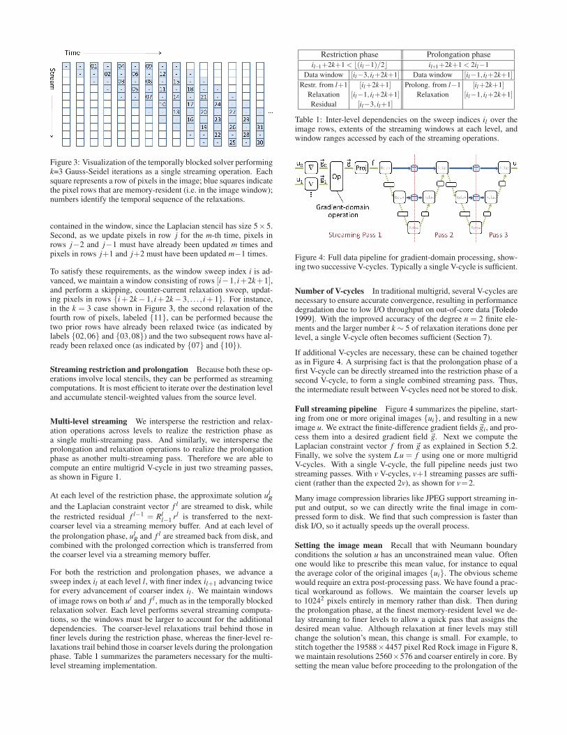
Figure 3: Visualization of the temporally blocked solver performingk=3 Gauss-Seidel iterations as a single streaming operation. Eachsquare represents a row of pixels in the image; blue squares indicatethe pixel rows that are memory-resident (i.e. in the image window);numbers identify the temporal sequence of the relaxations.

contained in the window, since the Laplacian stencil has size 5×5.Second, as we update pixels in row j for the m-th time, pixels inrows j−2 and j−1 must have already been updated m times andpixels in rows j+1 and j+2 must have been updated m−1 times.

To satisfy these requirements, as the window sweep index i is ad-vanced, we maintain a window consisting of rows [i−1, i+2k+1],and perform a skipping, counter-current relaxation sweep, updat-ing pixels in rows i + 2k− 1, i + 2k− 3, . . . , i + 1. For instance,in the k = 3 case shown in Figure 3, the second relaxation of thefourth row of pixels, labeled 11, can be performed because thetwo prior rows have already been relaxed twice (as indicated bylabels 02,06 and 03,08) and the two subsequent rows have al-ready been relaxed once (as indicated by 07 and 10).

Streaming restriction and prolongation Because both these op-erations involve local stencils, they can be performed as streamingcomputations. It is most efficient to iterate over the destination leveland accumulate stencil-weighted values from the source level.

Multi-level streaming We intersperse the restriction and relax-ation operations across levels to realize the restriction phase asa single multi-streaming pass. And similarly, we intersperse theprolongation and relaxation operations to realize the prolongationphase as another multi-streaming pass. Therefore we are able tocompute an entire multigrid V-cycle in just two streaming passes,as shown in Figure 1.

At each level of the restriction phase, the approximate solution ulR

and the Laplacian constraint vector f l are streamed to disk, while

the restricted residual f l−1 = Rll−1 rl is transferred to the next-

coarser level via a streaming memory buffer. And at each level of

the prolongation phase, ulR and f l are streamed back from disk, and

combined with the prolonged correction which is transferred fromthe coarser level via a streaming memory buffer.

For both the restriction and prolongation phases, we advance asweep index il at each level l, with finer index il+1 advancing twicefor every advancement of coarser index il . We maintain windows

of image rows on both ul and f l , much as in the temporally blockedrelaxation solver. Each level performs several streaming computa-tions, so the windows must be larger to account for the additionaldependencies. The coarser-level relaxations trail behind those infiner levels during the restriction phase, whereas the finer-level re-laxations trail behind those in coarser levels during the prolongationphase. Table 1 summarizes the parameters necessary for the multi-level streaming implementation.

Restriction phase Prolongation phase

il−1+2k+1 < ⌊(il−1)/2⌋ il+1+2k+1 < 2il−1

Data window [il−3, il+2k+1] Data window [il−1, il+2k+1]

Restr. from l+1 [il+2k+1] Prolong. from l−1 [il+2k+1]

Relaxation [il−1, il+2k+1] Relaxation [il−1, il+2k+1]

Residual [il−3, il+1]

Table 1: Inter-level dependencies on the sweep indices il over theimage rows, extents of the streaming windows at each level, andwindow ranges accessed by each of the streaming operations.

Figure 4: Full data pipeline for gradient-domain processing, show-ing two successive V-cycles. Typically a single V-cycle is sufficient.

Number of V-cycles In traditional multigrid, several V-cycles arenecessary to ensure accurate convergence, resulting in performancedegradation due to low I/O throughput on out-of-core data [Toledo1999]. With the improved accuracy of the degree n = 2 finite ele-ments and the larger number k∼ 5 of relaxation iterations done perlevel, a single V-cycle often becomes sufficient (Section 7).

If additional V-cycles are necessary, these can be chained togetheras in Figure 4. A surprising fact is that the prolongation phase of afirst V-cycle can be directly streamed into the restriction phase of asecond V-cycle, to form a single combined streaming pass. Thus,the intermediate result between V-cycles need not be stored to disk.

Full streaming pipeline Figure 4 summarizes the pipeline, start-ing from one or more original images ui, and resulting in a newimage u. We extract the finite-difference gradient fields~gi, and pro-cess them into a desired gradient field ~g. Next we compute theLaplacian constraint vector f from ~g as explained in Section 5.2.Finally, we solve the system Lu = f using one or more multigridV-cycles. With a single V-cycle, the full pipeline needs just twostreaming passes. With v V-cycles, v+1 streaming passes are suffi-cient (rather than the expected 2v), as shown for v=2.

Many image compression libraries like JPEG support streaming in-put and output, so we can directly write the final image in com-pressed form to disk. We find that such compression is faster thandisk I/O, so it actually speeds up the overall process.

Setting the image mean Recall that with Neumann boundaryconditions the solution u has an unconstrained mean value. Oftenone would like to prescribe this mean value, for instance to equalthe average color of the original images ui. The obvious schemewould require an extra post-processing pass. We have found a prac-tical workaround as follows. We maintain the coarser levels upto 10242 pixels entirely in memory rather than disk. Then duringthe prolongation phase, at the finest memory-resident level we de-lay streaming to finer levels to allow a quick pass that assigns thedesired mean value. Although relaxation at finer levels may stillchange the solution’s mean, this change is small. For example, tostitch together the 19588×4457 pixel Red Rock image in Figure 8,we maintain resolutions 2560×576 and coarser entirely in core. Bysetting the mean value before proceeding to the prolongation of the

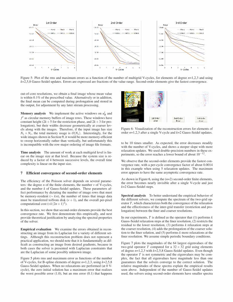
Figure 5: Plot of the rms and maximum errors as a function of the number of multigrid V-cycles, for elements of degree n=1,2,3 and usingk=2,5,8 Gauss-Seidel updates. Errors are expressed are fractions of the value range. Second-order elements give the fastest convergence.

out-of-core resolutions, we obtain a final image whose mean valueis within 0.1% of the prescribed value. Alternatively or in addition,the final mean can be computed during prolongation and stored inthe output, for adjustment by any later stream processing.

Memory analysis We implement the active windows on ulR and

f l as circular memory buffers of image rows. These windows haveconstant height (2k+5 for the restriction phase, and 2k+3 for pro-longation), but their widths decrease geometrically at coarser lev-els along with the images. Therefore, if the input image has sizeNx ×Ny, the total memory usage is O(Nx). Interestingly, for thewide images shown in Section 9, it would be more memory-efficientto sweep horizontally rather than vertically, but unfortunately thisis incompatible with the row-major ordering of image file formats.

Time analysis The amount of work at each multigrid level is lin-ear on the image size at that level. Because the system size is re-duced by a factor of 4 between successive levels, the overall timecomplexity is linear on the input size.

7 Efficient convergence of second-order elements

The efficiency of the Poisson solver depends on several parame-ters: the degree n of the finite elements, the number v of V-cycles,and the number k of Gauss-Seidel updates. These parameters af-fect performance by dictating the number of image rows that mustbe memory-resident (∼ k n), the number of times that image datamust be transferred to/from disk (v + 1), and the overall per-pixelcomputational cost (vk (2n+1)2).

In this section, we show that second-order elements provide the bestconvergence rate. We first demonstrate this empirically, and nextprovide theoretical justification by analyzing the spectral propertiesof the solver.

Empirical evaluation We examine the errors obtained in recon-structing an image from its Laplacian for a variety of different set-tings. Although this reconstruction problem does not represent apractical application, we should note that it is fundamentally as dif-ficult as constructing an image from desired gradients, because inboth cases the solver is presented with Laplacian constraints thatare the Laplacian of some possibly unknown image.

Figure 5 plots rms and maximum error as functions of the numberof V-cycles, for B-spline elements of degree n=1,2,3, using k=2,5,8Gauss-Seidel updates. When no relaxations are performed (at 0 V-cycle), the zero initial solution has a maximum error that realizesthe worst possible error (1.0), but an rms error (0.1) that happens

Figure 6: Visualization of the reconstruction errors for elements oforder n=1,2,3 after a single V-cycle and k=2 Gauss-Seidel updates.

to be 10 times smaller. As expected, the error decreases steadilywith the number of V-cycles, and shows a steeper slope with morerelaxation updates. We used double-precision numbers in these ex-periments, so the error reaches a lower bound of about 10−12.

We observe that the second-order elements provide the fastest con-vergence rate, with a per-cycle convergence factor of about 0.0014in this example when using 5 relaxation updates. The maximumerror appears to have the same asymptotic convergence rate.

As shown in Figure 6, using the (n=2) second-order finite elements,the error becomes nearly invisible after a single V-cycle and justk=2 Gauss-Seidel steps.

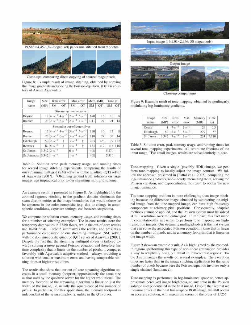
Spectral analysis To better understand the empirical behavior ofthe different solvers, we compute the spectrum of the two-grid op-erator T , which characterizes both the convergence of the relaxationand the effectiveness of the inter-grid transfer (restriction and pro-longation) between the finer and coarser resolutions.

In our experiments, T is defined as the operator that (1) performs kGauss-Seidel relaxation steps at the finer resolution, (2) restricts theresidual to the lower resolution, (3) performs k relaxation steps atthe coarser resolution, (4) adds the prolongation of the coarser solu-tion to the finer solution, and (5) performs k more relaxations at thefiner resolution. We assume simple periodic boundary conditions.

Figure 7 plots the magnitudes of the 64 largest eigenvalues of thetwo-grid operator T computed for a 32× 32 grid using elementsof degree n=1,2,3 with k=2,5,8 Gauss-Seidel updates. Even thoughthe operator T is not symmetric and the eigenvalues may be com-plex, the fact that all eigenvalues have magnitude less than oneguarantees that the solvers converge to the correct solution. Therelative magnitudes of these spectra explain the empirical resultsseen above. Independent of the number of Gauss-Seidel updatesused, the solvers using second-order elements have smaller spectra

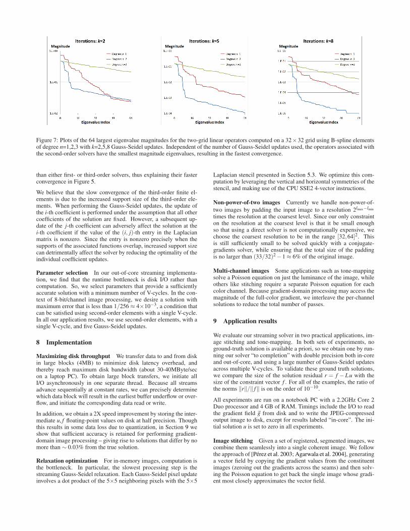
Figure 7: Plots of the 64 largest eigenvalue magnitudes for the two-grid linear operators computed on a 32×32 grid using B-spline elementsof degree n=1,2,3 with k=2,5,8 Gauss-Seidel updates. Independent of the number of Gauss-Seidel updates used, the operators associated withthe second-order solvers have the smallest magnitude eigenvalues, resulting in the fastest convergence.

than either first- or third-order solvers, thus explaining their fasterconvergence in Figure 5.

We believe that the slow convergence of the third-order finite el-ements is due to the increased support size of the third-order ele-ments. When performing the Gauss-Seidel updates, the update ofthe i-th coefficient is performed under the assumption that all othercoefficients of the solution are fixed. However, a subsequent up-date of the j-th coefficient can adversely affect the solution at thei-th coefficient if the value of the (i, j)-th entry in the Laplacianmatrix is nonzero. Since the entry is nonzero precisely when thesupports of the associated functions overlap, increased support sizecan detrimentally affect the solver by reducing the optimality of theindividual coefficient updates.

Parameter selection In our out-of-core streaming implementa-tion, we find that the runtime bottleneck is disk I/O rather thancomputation. So, we select parameters that provide a sufficientlyaccurate solution with a minimum number of V-cycles. In the con-text of 8-bit/channel image processing, we desire a solution withmaximum error that is less than 1/256≈ 4×10−3, a condition thatcan be satisfied using second-order elements with a single V-cycle.In all our application results, we use second-order elements, with asingle V-cycle, and five Gauss-Seidel updates.

8 Implementation

Maximizing disk throughput We transfer data to and from diskin large blocks (4MB) to minimize disk latency overhead, andthereby reach maximum disk bandwidth (about 30-40MByte/secon a laptop PC). To obtain large block transfers, we initiate allI/O asynchronously in one separate thread. Because all streamsadvance sequentially at constant rates, we can precisely determinewhich data block will result in the earliest buffer underflow or over-flow, and initiate the corresponding data read or write.

In addition, we obtain a 2X speed improvement by storing the inter-mediate u, f floating-point values on disk at half precision. Thoughthis results in some data loss due to quantization, in Section 9 weshow that sufficient accuracy is retained for performing gradient-domain image processing – giving rise to solutions that differ by nomore than ∼ 0.03% from the true solution.

Relaxation optimization For in-memory images, computation isthe bottleneck. In particular, the slowest processing step is thestreaming Gauss-Seidel relaxation. Each Gauss-Seidel pixel updateinvolves a dot product of the 5×5 neighboring pixels with the 5×5

Laplacian stencil presented in Section 5.3. We optimize this com-putation by leveraging the vertical and horizontal symmetries of thestencil, and making use of the CPU SSE2 4-vector instructions.

Non-power-of-two images Currently we handle non-power-of-

two images by padding the input image to a resolution 2lmax−lmin

times the resolution at the coarsest level. Since our only constrainton the resolution at the coarsest level is that it be small enoughso that using a direct solver is not computationally expensive, wechoose the coarsest resolution to be in the range [32,64]2. Thisis still sufficiently small to be solved quickly with a conjugate-gradients solver, while ensuring that the total size of the paddingis no larger than (33/32)2−1≈ 6% of the original image.

Multi-channel images Some applications such as tone-mappingsolve a Poisson equation on just the luminance of the image, whileothers like stitching require a separate Poisson equation for eachcolor channel. Because gradient-domain processing may access themagnitude of the full-color gradient, we interleave the per-channelsolutions to reduce the total number of passes.

9 Application results

We evaluate our streaming solver in two practical applications, im-age stitching and tone-mapping. In both sets of experiments, noground-truth solution is available a priori, so we obtain one by run-ning our solver “to completion” with double precision both in-coreand out-of-core, and using a large number of Gauss-Seidel updatesacross multiple V-cycles. To validate these ground truth solutions,we compare the size of the solution residual r = f − Lu with thesize of the constraint vector f . For all of the examples, the ratio ofthe norms ‖r‖/‖ f‖ is on the order of 10−10.

All experiments are run on a notebook PC with a 2.2GHz Core 2Duo processor and 4 GB of RAM. Timings include the I/O to readthe gradient field ~g from disk and to write the JPEG-compressedoutput image to disk, except for results labeled “in-core”. The ini-tial solution u is set to zero in all experiments.

Image stitching Given a set of registered, segmented images, wecombine them seamlessly into a single coherent image. We followthe approach of [Perez et al. 2003; Agarwala et al. 2004], generatinga vector field by copying the gradient values from the constituentimages (zeroing out the gradients across the seams) and then solv-ing the Poisson equation to get back the single image whose gradi-ent most closely approximates the vector field.

19,588×4,457 (87-megapixel) panorama stitched from 9 photos

Close-ups, comparing direct copying of source image pixels

Figure 8: Example result of image stitching, obtained by copyingthe image gradients and solving the Poisson equation. (Data is cour-tesy of Aseem Agarwala.)

Image Size Rms error Max error Mem. (MB) Time (s)

name (MP) SM QT SM QT SM QT SM QT

Streaming in-core solver

Beynac 12 4·10−5 4·10

−5 2·10−4 5·10

−3 670 16 10 8

Rainier 23 2·10−5 6·10

−5 2·10−4 4·10

−3 1311 27 21 14

Streaming out-of-core solver

Beynac 12 4·10−5 4·10

−5 3·10−4 5·10

−3 190 16 17 8

Rainier 23 3·10−5 6·10

−5 3·10−4 4·10

−3 110 27 33 14

Edinburgh 50 2·10−5 † 3·10

−4 † 203 123 79 122

Redrock 87 5·10−5 † 4·10

−4 † 133 112 118 118

St. James 3,342 2·10−4 6·10

−4 408 5,270

St. James(log) 3,342 1·10−4 1·10

−3 408 5,310

Table 2: Solution error, peak memory usage, and running timesfor several image stitching experiments, comparing the results ofour streaming multigrid (SM) solver with the quadtree (QT) solverof Agarwala [2007]. †Obtaining ground truth solutions on largeimages was impractical prior to our streaming multigrid scheme.

An example result is presented in Figure 8. As highlighted by thezoomed regions, stitching in the gradient domain eliminates theseam discontinuities at the image boundaries that would otherwisebe apparent in the color composite (e.g. due to change in atmo-spheric conditions, exposure settings, etc. between snapshots).

We compute the solution errors, memory usage, and running timesfor a number of stitching examples. The in-core results store thetemporary data values in 32-bit floats, while the out-of-core resultsuse 16-bit floats. Table 2 summarizes the results, and presents aperformance comparison of our streaming multigrid (SM) solverwith the domain-specific quadtree (QT) solver of Agarwala [2007].Despite the fact that the streaming multigrid solver is tailored to-wards solving a more general Poisson equation and therefore hastime complexity that is linear on the number of pixels, it comparesfavorably with Agarwala’s adaptive method – always providing asolution with smaller maximum error, and having comparable run-ning times at higher resolutions.

The results also show that our out-of-core streaming algorithm op-erates in a small memory footprint, approximately the same sizeas that used by the quadtree solver for the higher resolutions. Thememory footprint of the streaming algorithm is linear on just thewidth of the image, i.e. usually the square-root of the number ofpixels. In particular, for this application, the memory footprint isindependent of the seam complexity, unlike in the QT solver.

Input image (16,950×2,956; 50 megapixels)

Output image

Close-up comparisons

Figure 9: Example result of tone-mapping, obtained by nonlinearlymodulating log-luminance gradients.

Image Size Rms Max Memory Time

name (MP) error error (MB) (s)

Ocean† 1 7·10−5 2·10

−3 29 0.3

Edinburgh 50 2·10−3 5·10

−3 279 37

St. James 3,342 3·10−4 2·10

−3 224 2,710

Table 3: Solution error, peak memory usage, and running times forseveral tone-mapping experiments. All errors are fractions of theinput range. †For small images, results are solved entirely in-core.

Tone-mapping Given a single (possibly HDR) image, we per-form tone-mapping to locally adjust the image contrast. We fol-low the approach presented in [Fattal et al. 2002], computing thelog-luminance gradients, non-linearly attenuating them, solving thePoisson equation, and exponentiating the result to obtain the newimage luminance.

The tone mapping problem is more challenging than image stitch-ing because the difference image, obtained by subtracting the origi-nal image from the tone-mapped image, can have high-frequencycomponents at arbitrary pixel positions. Consequently, adaptivemethods cannot be applied, and the Poisson system must be solvedat full resolution over the entire grid. In the past, this fact madeit computationally infeasible to perform tone mapping on high-resolution images. Our streaming multigrid solver is the first systemthat can solve the associated Poisson equation in time that is linearon the number of pixels, and in a memory footprint that is linear onthe image width.

Figure 9 shows an example result. As is highlighted by the zoomed-in regions, performing this type of non-linear attenuation providesa way to adaptively bring out detail in low-contrast regions. Ta-ble 3 summarizes the results on several examples. The executiontimes are faster than in the image stitching application for the samenumber of pixels because here the Poisson equation involves only asingle channel (luminance).

Tone-mapping is performed in log-luminance space to better ap-proximate perceived image brightness, so any error in the Poissonsolution is exponentiated in the final image. Despite the fact that wemeasure errors in the final linear-space RGB image, we still obtainan accurate solution, with maximum errors on the order of 1/255.

(a) Mosaic of 643 input photographs with differing exposures

(b) Result of stitching the images in linear RGB space

(c) Result of stitching the images in log-RGB space

(d) Result of tone-mapping (c) in log-luminance space

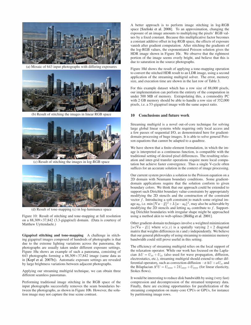
Figure 10: Result of stitching and tone-mapping at full resolutionon a 88,309×37,842 (3.3-gigapixel) domain. (Data is courtesy ofMatthew Uyttendaele.)

Gigapixel stitching and tone-mapping A challenge in stitch-ing gigapixel images composed of hundreds of photographs is thatdue to the extreme lighting variations across the panorama, thephotographs are usually taken under different exposure settings.Figure 10a shows an example of such a panorama, consisting of643 photographs forming a 88,309×37,842 image (same data asin [Kopf et al. 2007b]). Automatic exposure settings are revealedby large brightness variations between adjacent photographs.

Applying our streaming multigrid technique, we can obtain threedifferent seamless panoramas.

Performing traditional image stitching in the RGB space of theinput photographs successfully removes the seam boundaries be-tween the photographs, as shown in Figure 10b. However, the solu-tion image may not capture the true scene contrast.

A better approach is to perform image stitching in log-RGBspace [Szeliski et al. 2008]. To an approximation, changing theexposure of an image amounts to multiplying the pixels’ RGB val-ues by a fixed constant. Because this multiplicative factor becomesa constant additive offset in log-RGB space, the effects of exposurevanish after gradient computation. After stitching the gradients ofthe log-RGB values, the exponentiated Poisson solution gives theHDR image shown in Figure 10c. We observe that the rightmostportion of the image seems overly bright, and believe that this isdue to saturation in the source photographs.

Figure 10d shows the result of applying a tone-mapping operationto convert the stitched HDR result to an LDR image, using a secondapplication of the streaming multigrid solver. The error, memorysize, and execution time are shown in the last row of Table 3.

For this example dataset which has a row size of 88,000 pixels,our implementation can perform the entirety of the computation inunder 500 MB of memory. Extrapolating this, a commodity PCwith 2 GB memory should be able to handle a row size of 352,000pixels, i.e. a 53-gigapixel image with the same aspect ratio.

10 Conclusions and future work

Streaming multigrid is a novel out-of-core technique for solvinglarge global linear systems while requiring only local access anda few passes of sequential I/O, as demonstrated here for gradient-domain processing of huge images. It is able to solve general Pois-son equations that cannot be adapted to a quadtree.

We have shown that a finite-element formulation, in which the im-age is interpreted as a continuous function, is compatible with thetraditional setting of desired pixel differences. The resulting relax-ation and inter-grid transfer operations require more local compu-tation but achieve faster convergence. Thus a single V-cycle oftensuffices for an accurate solution in the context of image processing.

Our current system provides a solution to the Poisson equation on a2D domain with Neumann boundary conditions. Some gradient-domain applications require that the solution conform to givenboundary colors. We think that our approach could be extended tosupport such Dirichlet boundary value-constraints by appropriatelymodifying the 2D stencils and the construction of the constraintvector f . Introducing a soft constraint to match some original im-age u0, i.e. min‖∇u−~g‖2 +λ‖u−u0‖

2, may also be achievable bymodifying the 2D stencils and letting u0 contribute to f . Support-ing Dirichlet boundaries with irregular shape might be approachedusing a method akin to web-splines [Hollig et al. 2001].

Other gradient-domain techniques involve a weighted minimization‖w(∇u−~g)‖ where w(x,y) is a spatially varying 2× 2 diagonalmatrix that weights differences in x and y independently. We believethat our general philosophy of using streaming to minimize memorybandwidth could still prove useful in this setting.

The efficiency of streaming multigrid relies on the local support ofthe relaxation operator. While our work has focused on the Lapla-cian ∆U = Uxx +Uyy (also used for wave propagation, diffusion,electrostatics, etc.), streaming multigrid should extend to other dif-ferential operators, such as convection-diffusion−ε ∆U +aUx, andthe Bilaplacian ∆2U = Uxxxx +2Uxxyy +Uyyyy (for linear elasticity,Stokes flows).

It would be interesting to reduce disk bandwidth by using (very fast)compression and decompression of the streamed temporary data.Finally, there are exciting opportunities for parallelization of thestreaming computation on many-core CPUs or GPUs, for instanceby partitioning image rows.

Acknowledgments

We are very grateful to Aseem Agarwala and Matt Uyttendaele forsharing their aligned panorama images. We also thank Ketan Dalaland Bill Bolosky for valuable advice on implementing fast asyn-chronous I/O.

References

AGARWALA, A., DONTCHEVA, M., AGRAWALA, M., DRUCKER,S., COLBURN, A., CURLESS, B., SALESIN, D., AND COHEN,M. 2004. Interactive digital photomontage. ACM Transactionson Graphics (SIGGRAPH ’04), 294–302.

AGARWALA, A. 2007. Efficient gradient-domain compositingusing quadtrees. ACM Transactions on Graphics (SIGGRAPH’07).

AGRAWAL, A., RASKAR, R., NAYAR, S. K., AND LI, Y. 2005.Removing photography artifacts using gradient projection andflash-exposure sampling. ACM Transactions on Graphics (SIG-GRAPH ’05), 828–835.

BAE, S., PARIS, S., AND DURAND, F. 2006. Two-scale tone man-agement for photographic look. ACM Transactions on Graphics(SIGGRAPH ’06).

BOLITHO, M., KAZHDAN, M., BURNS, R., AND HOPPE, H.2007. Multilevel streaming for out-of-core surface reconstruc-tion. In Symposium on Geometry Processing, 69–78.

BOLZ, J., FARMER, I., GRINSPUN, E., AND SCHRODER, P. 2003.Sparse matrix solvers on the GPU: Conjugate gradients andmultigrid. ACM Transactions on Graphics (SIGGRAPH ’03),917–924.

BRANDT, A. 1977. Multi-level adaptive solutions to boundary-value problems. Mathematics of Computation 31, 333–390.

BRIGGS, W., HENSON, V., AND MCCORMICK, S. 2000. A Multi-grid Tutorial. Society for Industrial and Applied Mathematics.

CHRISTARA, C., AND SMITH, B. 1997. Multigrid and multilevelmethods for quadratic spline collocation. BIT 37, 4, 781–803.

DOUGLAS, C., HU, J., KOWARSCHIK, M., RUDE, U., AND

WEISS, C. 2000. Cache optimization for structured and un-structured grid multigrid. Electronic Transactions on NumericalAnalysis 10, 21–40.

FATTAL, R., LISCHINKSI, D., AND WERMAN, M. 2002. Gradientdomain high dynamic range compression. In ACM SIGGRAPH,249–256.

FINLAYSON, G., HORDLEY, S., AND DREW, M. 2002. Removingshadows from images. In European Conference on ComputerVision, 129–132.

FLETCHER, C. 1984. Computational Galerkin Methods. Springer.

GODDEKE, D., STRZODKA, R., MOHD-YUSOF, J., MC-CORMICK, P., WOBKER, H., BECKER, C., AND TUREK, S.2008. Using GPUs to improve multigrid solver performance ona cluster. Intnl. J. of Computational Science and Engineering.

GOODNIGHT, N., WOOLLEY, C., LEWIN, G., LUEBKE, D., AND

HUMPHREYS, G. 2003. A multigrid solver for boundary valueproblems using programmable graphics hardware. In Proc. ofGraphics Hardware, 102–111.

GORTLER, S., AND COHEN, M. 1995. Variational modeling withwavelets. In Symposium on Interactive 3D Graphics, 35–42.

HOLLIG, K., REIF, U., AND WIPPER, J. 2001. Weighted extendedB-spline approximation of Dirichlet problems. SIAM Journal onNumerical Analysis 39, 442–462.

HORN, B. 1974. Determining lightness from an image. ComputerGraphics and Image Processing 3, 277–299.

KAZHDAN, M., BOLITHO, M., AND HOPPE, H. 2006. Poissonsurface reconstruction. In Symposium on Geometry Processing,73–82.

KOPF, J., COHEN, M., LISCHINSKI, D., AND UYTTENDAELE,M. 2007. Joint bilateral upsampling. ACM Transactions onGraphics (SIGGRAPH ’07).

KOPF, J., UYTTENDAELE, M., DEUSSEN, O., AND COHEN, M.2007. Capturing and viewing gigapixel images. ACM Transac-tions on Graphics (SIGGRAPH ’07).

LEVIN, A., ZOMET, A., PELEG, S., AND WEISS, Y. 2004. Seam-less image stitching in the gradient domain. In European Con-ference on Computer Vision, 377–389.

LOSASSO, F., GIBOU, F., AND FEDKIW, R. 2004. Simulating wa-ter and smoke with an octree data structure. ACM Transactionson Graphics (SIGGRAPH ’04), 457–462.

MCCANN, J., AND POLLARD, N. 2008. Real-time gradient-domain painting. ACM Transactions on Graphics (SIGGRAPH’08).

PEREZ, P., GANGNET, M., AND BLAKE, A. 2003. Poisson imageediting. ACM Transactions on Graphics (SIGGRAPH ’03), 313–318.

PFEIFER, C. 1963. Data flow and storage allocation for the PDQ-5program on the Philco-2000. Communications of the ACM 6, 7,365–366.

SZELISKI, R., UYTTENDAELE, M., AND STEEDLY, D. 2008.Fast Poisson blending using multi-splines. Tech. Rep. MSR-TR-2008-58, Microsoft Research.

SZELISKI, R. 2006. Locally adapted hierarchical basis precon-ditioning. ACM Transactions on Graphics (SIGGRAPH ’06),1135–1143.

TOLEDO, S. 1999. A survey of out-of-core algorithms in numer-ical linear algebra. In External Memory Algorithms and Visual-ization, J. Abello and J. S. Vitter, Eds. American MathematicalSociety Press, Providence, RI, 161–180.

WEISS, Y. 2001. Deriving intrinsic images from image sequences.In International Conference on Computer Vision, 68–75.