STREAM: The Stanford Data StreamManagement System

Arvind Arasu, Brian Babcock, Shivnath Babu, John Cieslewicz, MayurDatar, Keith Ito, Rajeev Motwani, Utkarsh Srivastava, and Jennifer Widom

Department of Computer Science, Stanford UniversityContact author: widom@cs.stanford.edu

1 Introduction

Traditional database management systems are best equipped to run one-time queries over finite stored data sets. However, many modern applicationssuch as network monitoring, financial analysis, manufacturing, and sensor net-works require long-running, or continuous, queries over continuous unboundedstreams of data. In the STREAM project at Stanford, we are investigatingdata management and query processing for this class of applications. As partof the project we are building a general-purpose prototype Data Stream Man-agement System (DSMS), also called STREAM, that supports a large class ofdeclarative continuous queries over continuous streams and traditional storeddata sets. The STREAM prototype targets environments where streams maybe rapid, stream characteristics and query loads may vary over time, andsystem resources may be limited.

Building a general-purpose DSMS poses many interesting challenges:

• Although we consider streams of structured data records together withconventional stored relations, we cannot directly apply standard relationalsemantics to complex continuous queries over this data. In Sect. 2, wedescribe the semantics and language we have developed for continuousqueries over streams and relations.

• Declarative queries must be translated into physical query plans that areflexible enough to support optimizations and fine-grained scheduling deci-sions. Our query plans, composed of operators, queues, and synopses, aredescribed in Sect. 3.

• Achieving high performance requires that the DSMS exploit possibilitiesfor sharing state and computation within and across query plans. In ad-dition, constraints on stream data (e.g., ordering, clustering, referentialintegrity) can be inferred and used to reduce resource usage. In Sect. 4,we describe some of these techniques.

2 Arasu et al.

• Since data, system characteristics, and query load may fluctuate over thelifetime of a single continuous query, an adaptive approach to query exe-cution is essential for good performance. Our continuous monitoring andreoptimization subsystem is described in Sect. 5.

• When incoming data rates exceed the DSMS’s ability to provide exactresults for the active queries, the system should perform load-shedding byintroducing approximations that gracefully degrade accuracy. Strategiesfor approximation are discussed in Sect. 6.

• Due to the long-running nature of continuous queries, DSMS administra-tors and users require tools to monitor and manipulate query plans as theyrun. This functionality is supported by our graphical interface describedin Sect. 7.

Many additional problems, including exploiting parallelism and supportingcrash recovery, are still under investigation. Future directions are discussed inSect. 8.

2 The CQL Continuous Query Language

For simple continuous queries over streams, it can be sufficient to use a re-lational query language such as SQL, replacing references to relations withreferences to streams, and streaming new tuples in the result. However, ascontinuous queries grow more complex, e.g., with the addition of aggrega-tion, subqueries, windowing constructs, and joins of streams and relations,the semantics of a conventional relational language applied to these queriesquickly becomes unclear [3]. To address this problem, we have defined a for-mal abstract semantics for continuous queries, and we have designed CQL, aconcrete declarative query language that implements the abstract semantics.

2.1 Abstract Semantics

The abstract semantics is based on two data types, streams and relations,which are defined using a discrete, ordered time domain Γ :

• A stream S is an unbounded bag (multiset) of pairs 〈s, τ〉, where s is atuple and τ ∈ Γ is the timestamp that denotes the logical arrival time oftuple s on stream S.

• A relation R is a time-varying bag of tuples. The bag of tuples at timeτ ∈ Γ is denoted R(τ), and we call R(τ) an instantaneous relation. Notethat our definition of a relation differs from the traditional one which hasno built-in notion of time.

The abstract semantics uses three classes of operators over streams andrelations:

STREAM: The Stanford Data Stream Management System 3

Fig. 1. Data types and operator classes in abstract semantics.

• A relation-to-relation operator takes one or more relations as input andproduces a relation as output.

• A stream-to-relation operator takes a stream as input and produces arelation as output.

• A relation-to-stream operator takes a relation as input and produces astream as output.

Stream-to-stream operators are absent—they are composed from operators ofthe above three classes. These three classes are “black box” components of ourabstract semantics: the semantics does not depend on the exact operators inthese classes, but only on generic properties of each class. Figure 1 summarizesour data types and operator classes.

A continuous query Q is a tree of operators belonging to the above classes.The inputs of Q are the streams and relations that are input to the leafoperators, and the output of Q is the output of the root operator. The outputis either a stream or a relation, depending on the class of the root operator.At time τ , an operator of Q logically depends on its inputs up to τ : tuples ofSi with timestamps ≤ τ for each input stream Si, and instantaneous relationsRj(τ ′), τ ′ ≤ τ , for each input relation Rj . The operator produces new outputscorresponding to τ : tuples of S with timestamp τ if the output is a stream S,or instantaneous relation R(τ) if the output is a relation R. The behavior ofquery Q is derived from the behavior of its operators in the usual inductivefashion.

2.2 Concrete Language

Our concrete declarative query language, CQL (for Continuous Query Lan-guage), is defined by instantiating the operators of our abstract semantics.Syntactically, CQL is a relatively minor extension to SQL.

Relation-to-Relation Operators in CQL

CQL uses SQL constructs to express its relation-to-relation operators, andmuch of the data manipulation in a typical CQL query is performed usingthese constructs, exploiting the rich expressive power of SQL.

4 Arasu et al.

Stream-to-Relation Operators in CQL

The stream-to-relation operators in CQL are based on the concept of a slidingwindow [5] over a stream, and are expressed using a window specificationlanguage derived from SQL-99:

• A tuple-based sliding window on a stream S takes an integer N > 0 asa parameter and produces a relation R. At time τ , R(τ) contains the Ntuples of S with the largest timestamps ≤ τ . It is specified by followingS with “[Rows N].” As a special case, “[Rows Unbounded]” denotes theappend-only window “[Rows ∞].”

• A time-based sliding window on a stream S takes a time interval ω as aparameter and produces a relation R. At time τ , R(τ) contains all tuplesof S with timestamps between τ − ω and τ . It is specified by following Swith “[Range ω].” As a special case, “[Now]” denotes the window withω = 0.

• A partitioned sliding window on a stream S takes an integer N and a set ofattributes {A1, . . . , Ak} of S as parameters, and is specified by following Swith “[Partition By A1,...,Ak Rows N].” It logically partitions S intodifferent substreams based on equality of attributes A1, . . . , Ak, computesa tuple-based sliding window of size N independently on each substream,then takes the union of these windows to produce the output relation.

Relation-to-Stream Operators in CQL

CQL has three relation-to-stream operators: Istream, Dstream, and Rstream.Istream (for “insert stream”) applied to a relation R contains 〈s, τ〉 whenevertuple s is in R(τ) − R(τ − 1), i.e., whenever s is inserted into R at time τ .Dstream (for “delete stream”) applied to a relation R contains 〈s, τ〉 whenevertuple s is in R(τ − 1) − R(τ), i.e., whenever s is deleted from R at time τ .Rstream (for “relation stream”) applied to a relation R contains the 〈s, τ〉whenever tuple s is in R(τ), i.e., every current tuple in R is streamed at everytime instant.

Example CQL Queries

Example 1. The following continuous query filters a stream S:

Select Istream(*) From S [Rows Unbounded] Where S.A > 10

Stream S is converted into a relation by applying an unbounded (append-only)window. The relation-to-relation filter “S.A > 10” acts over this relation, andthe inserts to the filtered relation are streamed as the result. CQL includes anumber of syntactic shortcuts and defaults for convenience, which permit theabove query to be rewritten in the following more intuitive form:

STREAM: The Stanford Data Stream Management System 5

Select * From S Where S.A > 10

Example 2. The following continuous query is a windowed join of two streamsS1 and S2:

Select * From S1 [Rows 1000], S2 [Range 2 Minutes]Where S1.A = S2.A And S1.A > 10

The answer to this query is a relation. At any given time, the answer relationcontains the join (on attribute A with A > 10) of the last 1000 tuples of S1with the tuples of S2 that have arrived in previous 2 minutes. If we preferinstead to produce a stream containing new A values as they appear in thejoin, we can write “Istream(S1.A)” instead of “*” in the Select clause.

Example 3. The following continuous query probes a stored table R based oneach tuple in stream S and streams the result.

Select Rstream(S.A, R.B) From S [Now], R Where S.A = R.A

Complete details of CQL including syntax, semantic foundations, syntacticshortcuts and defaults, equivalences, and a comparison against related con-tinuous query languages are given in [3].

3 Query Plans and Execution

When a continuous query specified in CQL is registered with the STREAMsystem, a query plan is compiled from it. Query plans are composed of op-erators, which perform the actual processing, queues, which buffer tuples (orreferences to tuples) as they move between operators, and synopses, whichstore operator state.

3.1 Operators

Recall from Sect. 2 that there are two fundamental data types in our querylanguage: streams, defined as bags of tuple-timestamp pairs, and relations,defined as time-varying bags of tuples. We unify these two types in our imple-mentation as sequences of timestamped tuples, where each tuple additionallyis flagged as either an insertion (+) or deletion (−). We refer to the tuple-timestamp-flag triples as elements.

Streams only include + elements, while relations may include both +and − elements to capture the changing relation state over time. Queues log-ically contain sequences of elements representing either streams or relations.Each query plan operator reads from one or more input queues, processesthe input based on its semantics, and writes any output to an output queue.Individual operators may materialize their relational inputs in synopses (seeSect. 3.3) if such state is useful.

6 Arasu et al.

Name Operator Type Description

select relation-to-relation Filters elements based on predicate(s)project relation-to-relation Duplicate-preserving projectionbinary-join relation-to-relation Joins two input relationsmjoin relation-to-relation Multiway join from [22]union relation-to-relation Bag unionexcept relation-to-relation Bag differenceintersect relation-to-relation Bag intersectionantisemijoin relation-to-relation Antisemijoin of two input relationsaggregate relation-to-relation Performs grouping and aggregationduplicate-eliminate relation-to-relation Performs duplicate elimination

seq-window stream-to-relation Implements time-based, tuple-based,and partitioned windows

i-stream relation-to-stream Implements Istream semanticsd-stream relation-to-stream Implements Dstream semanticsr-stream relation-to-stream Implements Rstream semantics

Table 1. Operators used in STREAM query plans.

The operators in the STREAM system that implement the CQL languageare summarized in Table 1. In addition, there are several system operatorsto handle “housekeeping” tasks such as marshaling input and output andconnecting query plans together. During execution, operators are scheduledindividually, allowing for fine-grained control over queue sizes and query la-tencies. Scheduling algorithms are discussed later in Sect. 4.3.

3.2 Queues

A queue in a query plan connects its “producing” plan operator OP to its“consuming” operator OC . At any time a queue contains a (possibly empty)collection of elements representing a portion of a stream or relation. Theelements that OP produces are inserted into the queue and buffered thereuntil they are processed by OC .

Many of the operators in our system require that elements on their inputqueues be read in nondecreasing timestamp order. Consider, for example, awindow operator OW on a stream S as described in Sect. 2.2. If OW receivesan element 〈s, τ, +〉 and its input queue is guaranteed to be in nondecreasingtimestamp order, then OW knows it has received all elements with timestampτ ′ < τ , and it can construct the state of the window at time τ − 1. (If times-tamps are known to be unique it can construct the state at time τ .) If, onthe other hand, OW does not have this guarantee, it can never be sure it hasenough information to construct any window correctly. Thus, we require allqueues to enforce nondecreasing timestamps.

Mechanisms for buffering tuples and generating heartbeats to ensure non-decreasing timestamps, without sacrificing correctness or completeness, arediscussed in detail in [17].

STREAM: The Stanford Data Stream Management System 7

3.3 Synopses

Logically, a synopsis belongs to a specific plan operator, storing state that maybe required for future evaluation of that operator. (In our implementation,synopses are shared among operators whenever possible, as described laterin Sect. 4.1.) For example, to perform a windowed join of two streams, thejoin operator must be able to probe all tuples in the current window on eachinput stream. Thus, the join operator maintains one synopsis (e.g., a hashtable) for each of its inputs. On the other hand, operators such as selectionand duplicate-preserving union do not require any synopses.

The most common use of a synopsis in our system is to materialize thecurrent state of a (derived) relation, such as the contents of a sliding win-dow or the relation produced by a subquery. Synopses also may be used tostore a summary of the tuples in a stream or relation for approximate queryanswering, as discussed later in Sect. 6.2.

Performance requirements often dictate that synopses (and queues) mustbe kept in memory, and we tacitly make that assumption throughout thischapter. Our system does support overflow of these structures to disk, al-though currently it does not implement sophisticated algorithms for minimiz-ing I/O when overflow occurs, e.g., [20].

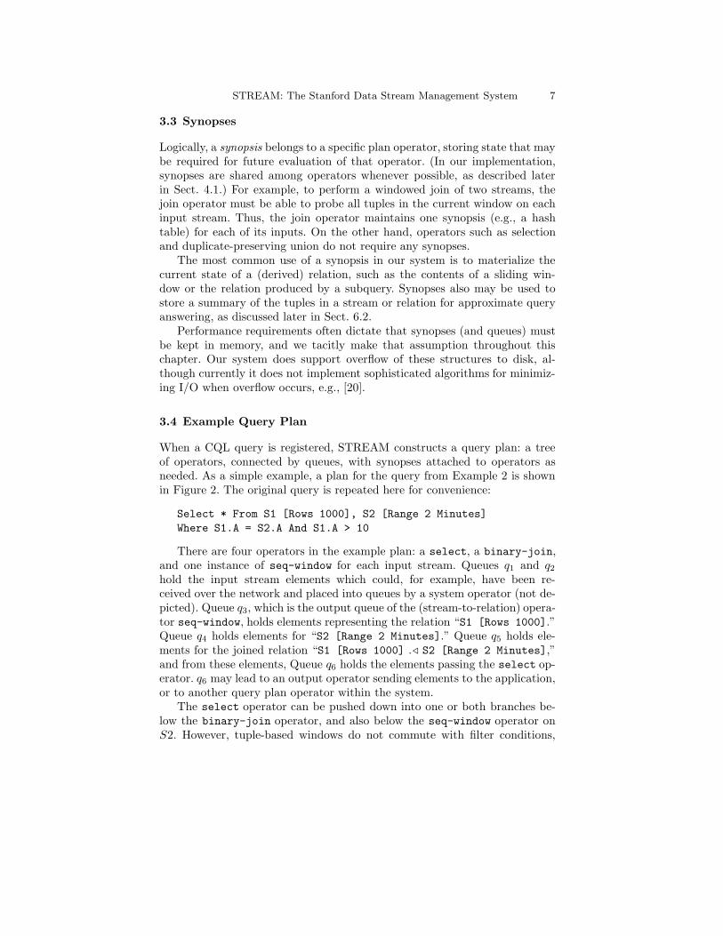
3.4 Example Query Plan

When a CQL query is registered, STREAM constructs a query plan: a treeof operators, connected by queues, with synopses attached to operators asneeded. As a simple example, a plan for the query from Example 2 is shownin Figure 2. The original query is repeated here for convenience:

Select * From S1 [Rows 1000], S2 [Range 2 Minutes]Where S1.A = S2.A And S1.A > 10

There are four operators in the example plan: a select, a binary-join,and one instance of seq-window for each input stream. Queues q1 and q2

hold the input stream elements which could, for example, have been re-ceived over the network and placed into queues by a system operator (not de-picted). Queue q3, which is the output queue of the (stream-to-relation) opera-tor seq-window, holds elements representing the relation “S1 [Rows 1000].”Queue q4 holds elements for “S2 [Range 2 Minutes].” Queue q5 holds ele-ments for the joined relation “S1 [Rows 1000] ./ S2 [Range 2 Minutes],”and from these elements, Queue q6 holds the elements passing the select op-erator. q6 may lead to an output operator sending elements to the application,or to another query plan operator within the system.

The select operator can be pushed down into one or both branches be-low the binary-join operator, and also below the seq-window operator onS2. However, tuple-based windows do not commute with filter conditions,

8 Arasu et al.

Fig. 2. A simple query plan illustrating operators, queues, and synopses.

and therefore the select operator cannot be pushed below the seq-windowoperator on S1.

The plan has four synopses, synopsis1–synopsis4. Each seq-window op-erator maintains a synopsis so that it can generate “−” elements when tuplesexpire from the sliding window. The binary-join operator maintains a syn-opsis materializing each of its relational inputs for use in performing joins withtuples on the opposite input, as described earlier. Since the select operatordoes not need to maintain any state, it does not have a synopsis.

Note that the contents of synopsis1 and synopsis3 are similar (as are thecontents of synopsis2 and synopsis4), since both maintain a materializationof the same window, but at slightly different positions of stream S1. Sect. 4.1discusses how we eliminate such redundancy.

3.5 Query Plan Execution

When a query plan is executed, a scheduler selects operators in the plan toexecute in turn. The semantics of each operator depends only on the times-tamps of the elements it processes, not on system or “wall-clock” time. Thus,the order of execution has no effect on the data in the query result, although itcan affect other properties such as latency and resource utilization. Schedulingis discussed further in Sect. 4.3.

Continuing with our example from the previous section, the seq-windowoperator on S1, on being scheduled, reads stream elements from q1. Supposeit reads element 〈s, τ, +〉. It inserts tuple s into synopsis1, and if the window

STREAM: The Stanford Data Stream Management System 9

is full (i.e., the synopsis already contains 1000 tuples), it removes the earliesttuple s′ in the synopsis. It then writes output elements into q3: the element〈s, τ, +〉 to reflect the addition of s to the window, and the element 〈s′, τ,−〉to reflect the deletion of s′ as it exits the window. Both of these events oc-cur logically at the same time instant τ . The other seq-window operator isanalogous.

When scheduled, the binary-join operator reads the earliest elementacross its two input queues. If it reads an element 〈s, τ, +〉 from q3, then itinserts s into synopsis3 and joins s with the contents of synopsis4, generatingoutput elements 〈s·t, τ, +〉 for each matching tuple t in synopsis4. Similarly,if the binary-join operator reads an element 〈s, τ,−〉 from q3, it generates〈s·t, τ,−〉 for each matching tuple t in synopsis4. A symmetric process occursfor elements read from q4. In order to ensure that the timestamps of its outputelements are nondecreasing, the binary-join operator must process its inputelements in nondecreasing timestamp order across both inputs.

Since the select operator is stateless, it simply dequeues elements fromq5, tests the tuple against its selection predicate, and enqueues the identicalelement into q6 if the test passes, discarding it otherwise.

4 Performance Issues

In the previous section we introduced the basic architecture of our query pro-cessing engine. However, simply generating the straightforward query plansand executing them as described can be very inefficient. In this section, we dis-cuss ways in which we improve the performance of our system by eliminatingdata redundancy (Sect. 4.1), selectively discarding data that will not be used(Sect. 4.2), and scheduling operators to most efficiently reduce intermediatestate (Sect. 4.3).

4.1 Synopsis Sharing

In Sect. 3.4, we observed that multiple synopses within a single query plan maymaterialize nearly identical relations. In Figure 2, synopsis1 and synopsis3

are an example of such a pair.We eliminate this redundancy by replacing the two synopses with light-

weight stubs, and a single store to hold the actual tuples. These stubs imple-ment the same interfaces as non-shared synopses, so operators can be oblivi-ous to the details of sharing. As a result, synopsis sharing can be enabled ordisabled on the fly.

Since operators are scheduled independently, it is likely that operatorssharing a single synopsis store will require slightly different views of the data.For example, if queue q3 in Figure 2 contains 10 elements, then synopsis3

will not reflect these changes (since the binary-join operator has not yetprocessed them), although synopsis1 will. When synopses are shared, logic in

10 Arasu et al.

Fig. 3. A query plan illustrating synopsis sharing.

the store tracks the progress of each stub, and presents the appropriate view(subset of tuples) to each of the stubs. Clearly the store must contain theunion of its corresponding stubs: A tuple is inserted into the store as soon asit is inserted by any one of the stubs, and it is removed only when it has beenremoved from all of the stubs.

To further decrease state redundancy, multiple query plans involving sim-ilar intermediate relations can share synopses as well. For example, supposethe following query is registered in addition to the query in Sect. 3.4:

Select A, Max(B) From S1 [Rows 200] Group By A

Since sliding windows are contiguous in our system, the window on S1 in thisquery is a subset of the window on S1 in the other query. Thus, the samedata store can be used to materialize both windows. The combination of thetwo query plans with both types of sharing is illustrated in Figure 3.

4.2 Exploiting Constraints

Streams may exhibit certain data or arrival patterns that can be exploitedto reduce run-time synopsis sizes. Such constraints can either be specifiedexplicitly at stream-registration time, or inferred by gathering statistics overtime [6]. (An alternate and more dynamic technique is for the streams tocontain punctuations, which specify run-time constraints that also can beused to reduce resource requirements [21].)

STREAM: The Stanford Data Stream Management System 11

As a simple example, consider a continuous query that joins a streamOrders with a stream Fulfillments based on attributes orderID and itemID,perhaps to monitor average fulfillment delays. In the general case, answeringthis query precisely requires synopses of unbounded size [2]. However, if weknow that all elements for a given orderID and itemID arrive on Orders beforethe corresponding elements arrive on Fulfillments, then we need not maintaina join synopsis for the Fulfillments operand at all. Furthermore, if Fulfillmentselements arrive clustered by orderID, then we need only save Orders tuplesfor a given orderID until the next orderID is seen.

We have identified several types of useful constraints over data streams.Effective optimizations can be made even when the constraints are not strictlymet by defining an adherence parameter, k, that captures how closely a givenstream or pair of streams adheres to a constraint of that type. We refer tothese as k-constraints:

• A referential integrity k-constraint on a many-one join between streamsdefines a bound k on the delay between the arrival of a tuple on the “many”stream and the arrival of its joining “one” tuple on the other stream.

• An ordered-arrival k-constraint on a stream attribute S.A defines a boundk on the amount of reordering in values of S.A. Specifically, given anytuple s in stream S, for all tuples s′ that arrive at least k + 1 elementsafter s, it must be true that s′.A ≥ s.A.

• A clustered-arrival k-constraint on a stream attribute S.A defines a boundk on the distance between any two elements that have the same value ofS.A.

We have developed query plan construction and execution algorithms thattake stream constraints into account in order to reduce synopsis sizes at queryoperators by discarding unnecessary state [9]. The smaller the value of k foreach constraint, the more state that can be discarded. Furthermore, if anassumed k-constraint is not satisfied by the data, our algorithm produces anapproximate answer whose error is proportional to the degree of deviation ofthe data from the constraint.

4.3 Operator Scheduling

An operator consumes elements from its input queues and produces elementson its output queue. Thus, the global operator scheduling policy can have alarge effect on memory utilization, particularly with bursty input streams.

Consider the following simple example. Suppose we have a query planwith two operators, O1 followed by O2. Assume that O1 takes one time unitto process a batch of n elements, and it produces 0.2n output elements perinput batch (i.e., its selectivity is 0.2). Further, assume that O2 takes one timeunit to operate on 0.2n elements, and it sends its output out of the system.(As far as the system is concerned, O2 produces no elements, and therefore

12 Arasu et al.

its selectivity is 0.) Consider the following bursty arrival pattern: n elementsarrive at every time instant from t = 0 to t = 6, then no elements arrive fromtime t = 7 through t = 13.

Under this scenario, consider the following scheduling strategies:

• FIFO scheduling: When batches of n elements have been accumulated,they are passed through both operators in two consecutive time units,during which no other element is processed.

• Greedy scheduling: At any time instant, if there is a batch of n elementsbuffered before O1, it is processed in one time unit. Otherwise, if thereare more than 0.2n elements buffered before O2, then 0.2n elements areprocessed using one time unit. This strategy is “greedy” since it givespreference to the operator that has the greatest rate of reduction in totalqueue size per unit time.

The following table shows the expected total queue size for each strategy,where each table entry is a multiplier for n.

Time 0 1 2 3 4 5 6 AvgFIFO scheduling 1.0 1.2 2.0 2.2 3.0 3.2 4.0 2.4Greedy scheduling 1.0 1.2 1.4 1.6 1.8 2.0 2.2 1.6

After time t = 6, input queue sizes for both strategies decline until they reach0 after time t = 13. The greedy strategy performs better because it runs O1

whenever it has input, reducing queue queue size by 0.8n elements each timestep, while the FIFO strategy alternates between executing O1 and O2.

However, the greedy algorithm has its shortcomings. Consider a plan withoperators O1, O2, and O3. O1 produces 0.9n elements per n input elements inone time unit, O2 processes 0.9n elements in one time unit without changingthe input size (i.e., it has selectivity 1), and O3 processes 0.9n elements inone time unit and sends its output out of the system (i.e., it has selectivity0). Clearly, the greedy algorithm will prioritize O3 first, followed by O1, andthen O2. If we consider the arrival pattern in the previous example then ourtotal queue size is as follows (again as multipliers for n):

Time 0 1 2 3 4 5 6 AvgFIFO scheduling 1.0 1.9 2.9 3.0 3.9 4.9 5.0 3.2Greedy scheduling 1.0 1.9 2.8 3.7 4.6 5.5 6.4 3.7

In this case, the FIFO algorithm is better. Under the greedy strategy,although O3 has highest priority, sometimes it is “blocked” from runningbecause it is preceded by O2, the operator with the lowest priority. If O1, O2

and O3 are viewed as a single block, then together they reduce n elementsto zero elements over three units of time, for an average reduction of 0.33nelements per unit time—better than the reduction rate of 0.1n elements O1

provides. Since the greedy algorithm considers individual operators only, itdoes not take advantage of this fact.

STREAM: The Stanford Data Stream Management System 13

Fig. 4. Adaptive query processing.

This observation forms the basis of our chain scheduling algorithm [4]. Ouralgorithm forms blocks (“chains”) of operators as follows: Start by markingthe first operator in the plan as the “current” operator. Next, find the blockof consecutive operators starting at the “current” operator that maximizesthe reduction in total queue size per unit time. Mark the first operator fol-lowing this block as the “current” operator and repeat the previous step untilall operators have been assigned to chains. Chains are scheduled accordingto the greedy algorithm, but within a chain, execution proceeds in FIFO or-der. In terms of overall memory usage, this strategy is provably close to theoptimal “clairvoyant” scheduling strategy, i.e., the optimal strategy based onknowledge of future input [4].

5 Adaptivity

In long-running stream applications, data and arrival characteristics of streamsmay vary significantly over time [13]. Query loads and system conditionsmay change as well. Without an adaptive approach to query processing, per-formance may drop drastically over time as the environment changes. TheSTREAM system includes a monitoring and adaptive query processing in-frastructure called StreaMon [10].

StreaMon has three components as shown in Figure 4(a): an Executor,which runs query plans to produce results, a Profiler, which collects andmaintains statistics about stream and plan characteristics, and a Reoptimizer,which ensures that the plans and memory structures are the most efficient forcurrent characteristics. In many cases, we combine the profiler and executorto reduce the monitoring overhead.

The Profiler and Reoptimizer are essential for adaptivity, but they competefor resources with the Executor. We have identified a clear three-way tradeoffamong run-time overhead, speed of adaptivity, and provable convergence to

14 Arasu et al.

good strategies if conditions stabilize. StreaMon supports multiple adaptivealgorithms that lie at different points along this tradeoff spectrum.

StreaMon can detect useful k-constraints (recall Sect. 4.2) in streams andexploit them to reduce memory requirements for many continuous queries.In addition, it can adaptively adjust the adherence parameter k based on theactual data in the streams. Figure 4(b) shows the portions of StreaMon’s Pro-filer and Reoptimizer that handle k-constraints, referred to as k-Mon. Whena query is registered, the optimizer notifies the profiler of potentially usefulconstraints. As the executor runs the query, the profiler monitors the inputstreams continuously and informs the reoptimizer whenever it detects a changein a k value for any of these constraints. The reoptimizer component adaptsto these changes by adding or dropping constraints used by the executor andadjusting k values used for memory allocation.

StreaMon also implements an algorithm called Adaptive Greedy (or A-Greedy) [7], which maintains join orders adaptively for pipelined multiwaystream joins, also known as MJoins [22]. Figure 4(c) shows the portionsof StreaMon’s Profiler and Reoptimizer that comprise the A-Greedy algo-rithm. Using A-Greedy, StreaMon monitors conditional selectivities and or-ders stream joins to minimize overall work in current conditions. In addition,StreaMon detects when changes in conditions may have rendered current or-derings suboptimal, and reorders in those cases. In stable conditions, the or-derings converged on by the A-Greedy algorithm are equivalent to those se-lected by a static Greedy algorithm that is provably within a cost factor < 4of optimal. In practice, the Greedy algorithm, and therefore A-Greedy, nearlyalways finds the optimal orderings.

In addition to adaptive join ordering, we use StreaMon to adaptively addand remove subresult caches in stream join plans, to avoid recomputation ofintermediate results [8]. StreaMon monitors costs and benefits of candidatecaches, selects caches to use, allocates memory to caches, and adapts over theentire spectrum between stateless MJoins and cache-rich join trees, as streamand system conditions change.

Currently we are in the process of applying the StreaMon approach tomake even more aspects of the STREAM system adaptive, including sharingof synopses and subplans, and operator scheduling.

6 Approximation

In many applications data streams can be bursty, with unpredictable peaksduring which the load may exceed available system resources, especially if nu-merous complex queries have been registered. Fortunately, for many streamapplications (e.g., in many monitoring tasks), it is acceptable to degrade ac-curacy gracefully by providing approximate answers during load spikes [18].

There are two primary ways in which a DSMS may be resource-limited:

STREAM: The Stanford Data Stream Management System 15

• CPU-limited (Sect. 6.1) – The data arrival rate may be so high that thereis insufficient CPU time to process each stream element. In this case, thesystem may approximate by dropping elements before they are processed.

• Memory-limited (Sect. 6.2) – The total state required for all registeredqueries may exceed available memory. In this case, the system may selec-tively retain some state, discarding the rest.

6.1 CPU-Limited Approximation

CPU usage can be reduced by load-shedding—dropping elements from queryplans and saving the CPU time that would be required to process them tocompletion. We implement load-shedding by introducing sampling operatorsthat probabilistically drop stream elements as they are input to the queryplan.

The time-accuracy tradeoffs for sampling are more understandable forsome query plans than others. For example, if we know a few basic statisticson the distribution of values in our streams, probabilistic guarantees on the ac-curacy of sliding-window aggregation queries for a given sampling rate can bederived mathematically, as we will show in below. However, in more complexqueries—ones involving joins, for example—the error introduced by samplingis less clear and the choice of error metric may be application-dependent.

Suppose we have a set of sliding-window aggregation queries over the inputstreams. A simple example is:

Select Avg(Temp) From SensorReadings [Range 5 Minutes]

If we have many such queries in a CPU-limited setting, our goal is to samplethe inputs so as to minimize the maximum relative error across all queries.(As an extension, we can weight the relative errors to provide “quality-of-service” distinctions.) It follows that we should select sampling rates suchthat the relative error is the same for all queries. Assume that for a givenquery Qi we know the mean µi and standard deviation σi of the values we areaggregating, as well as the window size Ni. These statistics can be collectedby the profiler component in the StreaMon architecture (recall Sect. 5). Wecan use the Hoeffding inequality [16] to derive a bound on the probability δthat our relative error exceeds a given threshold εmax for a given samplingrate. We then fix δ at a low value (e.g., 0.01) and algebraically manipulatethis equation to derive the required sampling rate Pi [6]:

Pi =1

εmax

√σ2

i + µ2i

2Niµ2i

log2δ

Our load-shedding policy solves for the best achievable εmax given theconstraint that the system, after inserting load-shedders, can keep up withthe arrival of elements. It then adds sampling operators at various points inthe query plan such that effective sampling rate for a query Qi is Pi.

16 Arasu et al.

6.2 Memory-Limited Approximation

Even using our scheduling algorithm that minimizes memory devoted toqueues (Sect. 4.3), and our constraint-aware execution strategy that mini-mizes synopsis sizes (Sect. 4.2), if we have many complex queries with largewindows (e.g., large tuple-based windows, or any size time-based windowsover rapid data streams), memory may become a constraint. Spilling to diskmay not be a feasible option due to online performance requirements.

In this scenario, memory usage can be reduced at the cost of accuracyby reducing the size of synopses at one or more operators. Incorporating awindow into a synopsis where no window is being used, or shrinking theexisting window, will shrink the synopsis. Note that if sharing is in place(Sect. 4.1), then modifying a single synopsis may affect multiple queries.

Reducing the size of a synopsis generally tends to also reduce the sizesof synopses above it in the query plan, but there are exceptions. Consider aquery plan where a sliding-window synopsis is used by a duplicate-eliminationoperator. Shrinking the window size can increase the operator’s output rate,leading to an increase in the size of “later” synopses. Fortunately, most ofthese cases can be detected statically when the query plan is generated, andthe system can avoid reducing synopsis sizes in such cases.

There are other methods for reducing synopsis size, including maintaininga sample of the intended synopsis content (which is not always equivalentto inserting a sample operator into the query plan), using histograms [19] orwavelets [12] when the synopsis is used for aggregation or even for a join,and using Bloom filters [11] for duplicate elimination, set difference, or setintersection. In addition, synopsis sizes can be reduced by lowering the kvalues for known k-constraints (Sect. 4.2). Lower k values cause more state tobe discarded, but result in loss of accuracy if the constraint does not hold forthe assumed k. All of these techniques share the property that memory use isflexible, and it can be traded against precision statically or dynamically.

See Sect. 8.3 for discussion on future directions related to approximation.

7 The STREAM System Interface

In a system for continuous queries, it is important for users, system admin-istrators, and system developers to have the ability to inspect the systemwhile it is running and to experiment with adjustments. To meet these needs,we have developed a graphical query and system visualizer for the STREAMsystem. The visualizer allows the user to:

• View the structure of query plans and their component entities (operators,queues, and synopses). Users can view the path of data flow through eachquery plan as well as the sharing of computation and state within the plan.

STREAM: The Stanford Data Stream Management System 17

Fig. 5. Screenshot of the STREAM visualizer.

• View the detailed properties of each entity. For example, the user caninspect the amount of memory being used (for queue and synopsis entities),the current throughput (for queue and operator entities), selectivity ofpredicates (for operator entities), and other properties.

• Dynamically adjust entity properties. These changes are reflected in thesystem in real time. For example, an administrator may choose to increasethe size of a queue to better handle bursty arrival patterns.

• View monitoring graphs that display time-varying entity properties suchas queue sizes, throughput, overall memory usage, and join selectivity,plotted dynamically against time.

A screenshot of our visualizer is shown in Figure 5. The large pane atthe left displays a graphical representation of a currently selected query plan.The particular query shown is a windowed join over two streams, R and S.Each entity in the plan is represented by an icon: the ladder-shaped iconsare queues, the boxes with magnifying glasses over them are synopses, thewindow panes are windowing operators, and so on. In this example, the userhas added three monitoring graphs: the rate of element flow through queuesabove and below the join operator, and the selectivity of the join.

The upper-right pane displays the property-value table for a currentlyselected entity. The user can inspect this list and can alter the values of someof the properties interactively. Finally, the lower-right pane displays a legendof entity icons and descriptions for reference.

Our technique for implementing the monitoring graphs shown in Fig-ure 5 is based on introspection queries on a special system stream called

18 Arasu et al.

SysStream. Every entity can publish any of its property values at any timeonto SysStream. When a specific dynamic monitoring task is desired, e.g.,monitoring recent join selectivity, the relevant entity writes its statistics pe-riodically on SysStream. Then a standard CQL query, typically a windowedaggregation query, is registered over SysStream to compute the desired con-tinuous result, which is fed to the monitoring graph in the visualizer. Usersand applications can also register arbitrary CQL queries over SysStream forcustomized monitoring tasks.

8 Future Directions

At the time of writing we plan to pursue the following general directions offuture work.

8.1 Distributed Stream Processing

So far we have considered a centralized DSMS model where all processingtakes place at a single system. In many applications the stream data is actu-ally produced at distributed sources. Moving some processing to the sourcesinstead of moving all data to a central system may lead to more efficient useof processing and network resources. Many new challenges arise if we wish tobuild a fully distributed data stream system with capabilities equivalent toour centralized system.

8.2 Crash Recovery

The ability to recover to a consistent state following a system crash is a keyfeature of conventional database systems, but has yet to be investigated fordata stream systems. There are some fundamental differences between DBMSsand DSMSs that play important role in crash recovery:

• The notion of consistent state in a DBMS is defined based on transac-tions, which are closely tied to the conventional one-time query model.ACID transactional properties do not map directly to the continuous queryparadigm.

• In a DBMS, the data in the database cannot change during down-time. Incontrast, many stream applications deliver data to the DSMS from outsidesources that do not stop generating data while the system is down, possiblyrequiring the DSMS to “catch up” following a crash.

• In a DBMS, queries underway at the time of a crash may be forgotten—it isthe responsibility of the application to restart them. In contrast, registeredcontinuous queries are part of the persistent state of a DSMS.

STREAM: The Stanford Data Stream Management System 19

These differences lead us to believe that new mechanisms are needed for crashrecovery in data stream systems. While logging of some type and perhapseven some notion of transactions may form a component of the solution, newtechniques will be required as well.

8.3 Improved Approximation

Although some aspects of the approximation problem have already been ad-dressed (see Sect. 6), more work is needed to address the problem in its fullgenerality. In the memory-limited case, work is needed on the problem of sam-pling over arbitrary subqueries, computing “maximum-subset” as opposed tosampling approximations, and maximizing accuracy over multiple weightedqueries. In the CPU-limited case, we need to address a broader range ofqueries, especially considering joins. Finally, we need to handle situationswhen the DSMS may be both CPU and memory-limited.

A significant challenge related to approximation is developing mechanismswhereby the system can indicate to users or applications that approximation isoccurring, and to what degree. The converse is also important: mechanisms forusers to indicate acceptable degrees of approximation. As one step in the latterdirection, we are developing extensions to CQL that enable the specification of“approximation guidelines” so that the user can indicate acceptable tolerancesand priorities.

8.4 Relationship to Publish-Subscribe Systems

In a publish-subscribe (pub-sub) system, e.g., [1, 14, 15], events may be pub-lished continuously, and they are forwarded by the system to users who haveregistered matching subscriptions. Clearly we can map a pub-sub system toa DSMS by considering publications as streams and subscriptions as continu-ous queries. However, the techniques we have developed so far for processingcontinuous queries in a DSMS have been geared primarily toward a relativelysmall number of independent, complex queries, while a pub-sub system haspotentially millions of simple, similar queries. We are exploring techniques tobridge the capabilities of the two: From the pub-sub perspective, provide asystem that supports a more general model of subscriptions. From the DSMSperspective, extend our approach to scale to an extremely larger number ofqueries.

References

1. M. K. Aguilera, R. E. Strom, D. C. Sturman, M. Astley, and T. D. Chandra.Matching events in a content-based subscription system. In Proc. of the 18thAnnual ACM Symp. on Principles of Distributed Computing, pages 53–61, May1999.

20 Arasu et al.

2. A. Arasu, B. Babcock, S. Babu, J. McAlister, and J. Widom. Characterizingmemory requirements for queries over continuous data streams. ACM Trans.on Database Systems, 29(1):1–33, Mar. 2004.

3. A. Arasu, S. Babu, and J. Widom. The CQL Continuous Query Language:Semantic Foundations and Query Execution. Technical report, Stanford Uni-versity, Oct. 2003. http://dbpubs.stanford.edu/pub/2003-67.

4. B. Babcock, S. Babu, M. Datar, and R. Motwani. Chain: Operator schedulingfor memory minimization in data stream systems. In Proc. of the 2003 ACMSIGMOD Intl. Conf. on Management of Data, pages 253–264, June 2003.

5. B. Babcock, S. Babu, M. Datar, R. Motwani, and J. Widom. Models and issuesin data stream systems. In Proc. of the 21st ACM SIGACT-SIGMOD-SIGARTSymp. on Principles of Database Systems, pages 1–16, June 2002.

6. B. Babcock, M. Datar, and R. Motwani. Load shedding for aggregation queriesover data streams. In Proc. of the 20th Intl. Conf. on Data Engineering, Mar.2004.

7. S. Babu, R. Motwani, K. Munagala, I. Nishizawa, and J. Widom. Adaptiveordering of pipelined stream filters. In Proc. of the 2004 ACM SIGMOD Intl.Conf. on Management of Data, June 2004.

8. S. Babu, K. Munagala, J. Widom, and R. Motwani. Adaptive caching forcontinuous queries. Technical report, Stanford University, Mar. 2004. http:

//dbpubs.stanford.edu/pub/2004-14.9. S. Babu and J. Widom. Exploiting k-constraints to reduce memory overhead

in continuous queries over data streams. Technical report, Stanford University,Nov. 2002. http://dbpubs.stanford.edu/pub/2002-52.

10. S. Babu and J. Widom. StreaMon: an adaptive engine for stream query process-ing. In Proc. of the 2004 ACM SIGMOD Intl. Conf. on Management of Data,June 2004. Demonstration description.

11. B. H. Bloom. Space/time trade-offs in hash coding with allowable errors. Com-munications of the ACM, 13(7):422–426, July 1970.

12. K. Chakrabarti, M. N. Garofalakis, R. Rastogi, and K. Shim. Approximatequery processing using wavelets. In Proc. of the 26th Intl. Conf. on Very LargeData Bases, pages 111–122, Sept. 2000.

13. J. Gehrke (ed). Data stream processing. IEEE Computer Society Bulletin ofthe Technical Comm. on Data Engg., 26(1), Mar. 2003.

14. F. Fabret, H-. A. Jacobsen, F. Llirbat, J. Pereira, K. A. Ross, and D. Shasha.Filtering algorithms and implementation for very fast publish/subscribe. InProc. of the 2000 ACM SIGMOD Intl. Conf. on Management of Data, pages115–126, May 2001.

15. R. E. Gruber, B. Krishnamurthy, and E. Panagos. READY: A high performanceevent notification system. In Proc. of the 16th Intl. Conf. on Data Engineering,pages 668–669, Mar. 2000.

16. W. Hoeffding. Probability inequalities for sums of bounded random variables.Journal of American Statistical Society, 58(301):13–30, March 1963.

17. U. Srivastava and J. Widom. Flexible time management in data stream systems.In Proc. of the 23rd ACM SIGACT-SIGMOD-SIGART Symp. on Principles ofDatabase Systems, June 2004.

18. N. Tatbul, U. Cetintemel, S. B. Zdonik, M. Cherniak, and M. Stonebraker. Loadshedding in a data stream manager. In Proc. of the 29th Intl. Conf. on VeryLarge Data Bases, pages 309–320, Sept. 2003.

STREAM: The Stanford Data Stream Management System 21

19. N. Thaper, S. Guha, P. Indyk, and N. Koudas. Dynamic multidimensionalhistograms. In Proc. of the 2002 ACM SIGMOD Intl. Conf. on Management ofData, pages 428–439, June 2002.

20. D. Thomas and R. Motwani. Caching queues in memory buffers. In Proc. ofthe 15th Annual ACM-SIAM Symp. on Discrete Algorithms, Jan. 2004.

21. P. A. Tucker, D. Maier, T. Sheard, and L. Fegaras. Exploiting punctuationsemantics in continuous data streams. IEEE Trans. on Knowledge and DataEngg., 15(3):555–568, May 2003.

22. S. Viglas, J. F. Naughton, and J. Burger. Maximizing the output rate of multi-way join queries over streaming information sources. In Proc. of the 29th Intl.Conf. on Very Large Data Bases, pages 285–296, Sept. 2003.