STRATIFICATION DYNAMICS AND GRAVITATIONAL … burau, & stacey: circulation stratification dynamics...

MONISMITH, BURAU, & STACEY: CIRCULATION

STRATIFICATION DYNAMICS AND GRAVITATIONAL CIRCULATION IN NORTHERN SAN FRANCISCO BAY

STEPHEN MONISMITH, JON R. BURAU AND MARK STACEY

Environmental Fluid Mechanics Laboratory Stanford University, Stanford CA 94305-4020

In this paper we discuss field observations and modeling results examining the connection between flow-induced stratification and gravitational circulation. We present simultaneous ADCP and top and bottom salinity records collected by the USGS showing that density-driven flows are highly inter- mittent, with strong gravitational circulation accompanying stratification episodes. Tidal variations in gravitational circulation appear to be linked to tide-induced vertical mixing and to the strain-induced periodic stratification (SIPS) that i s typically found in Northern San Francisco Bay. Results obtained using a ID water column model suggest that there exists a critical condition where tidal mixing is unable to overcome the creation of stratification by advection. Variability of observed stratification i s better explained by a parameter which explicitly considers SIPS, and thus which depends explicitly on the longitudinal salinity gradient, than i t i s by a similar parameter based on flow.

The tides and tidal currents in San Francisco Bay are extremely energetic. At the Golden Gate, sea level can change as much as 2.6 m in - 6 hours on a spring tide. Because of the geometry of the Bay, these elevations can drive maximal tidal currents in the channels ofSan Francisco Bay in the range of 50 to 200 c d s (Cheng & Gartner 1984). The magnitude of the energy input by the tides sets the stage for most of the transport and mixing processes that provide the dominant linkage between physical forcing, e.g., river flow, and biological response, e.g., annual primary production by phytoplankton.

Biologically relevant transport and mixing processes include those associated with vertical turbulent mixing (i.e., over depth), horizontal advection (e.g., landward or seaward) or dispersion by some combination of mixing and advection (Fischer etal. 1979). Reviews ofhorizontal dispersion mechanisms associated with tides, e.g., depth-averaged Eulerian residual currents or by wave-induced transport in San Francisco Bay can be found in Walters et al. (1985). In this paper we focus on stratification dynamics and gravitational circulation, with particular attention to northern San Francisco Bay (see Fig. 1). We focus on stratification because rates of vertical mixing can be much smaller in the presence of stratification than in an homogeneous water column (see e.g., Abraham 1988 or Ivey & lmberger 1992). Hence, biological processes that are affected by vertical exchanges should be dependent on water column stability. We examine gravitational circulation, flows driven by baroclinic pressure gradients, because they are thought to be a primary influence on the longitudinal transport of organisms (Herbold et al. 1992), and on the formation of the Estuarine Turbidity Maximum (ETM -see below). The pairing of gravitational circulation with stratification is not an arbitrary choice: as we will discuss below, the two are strongly connected. Moreover, both are likely

123

SAN FRANCISCO BAY: THE ECOSYSTEM MONISMITH, BURAU, & STACEY: CIRCULATION

2 0 3

L

to be directly influenced by the buoyancy input provided by Delta inflow to the Bay, and thus to represent a means by which inflows to the Bay might influence ecological processes.

Before presenting our observations, in $2 we attempt to make the case that dynamics of density stratification are relevant to ecological processes in San Francisco Bay, both directly, and through their influence on gravitational circulation. In $3 we use simultaneous observations of salinity and velocity structure to show that gravitational circulation and stratification are, in fact, strongly linked to each other and to the tides, with flow playing a somewhat secondary role. We pursue this coupling using a one-dimensional model of salinity and velocity structure in $4, finding that there appears to be a critical condition, which can be described using a parameter, Ri,, determined by the tides and by the longitudinal structure of the salinity field, which separates episodes of strong, persistent stratification, intense gravitational circulation and substantial upstream salt flux, from periods in which all of these are relatively weak. We summarize and discuss our findings in $5 .

2. DENSITY STRATIFICATION IN SAN FRANCISCO BAY 2.1. Linkage of stratification and primary production by phytoplankton In seeking to explain his observations of spring phytoplankton blooms in South

San Francisco Bay, where sufficiently strong benthic grazing appeared to be available to consume any and all primary production, and equally, where there was no obvious nutrient limitation to suppress blooms, Cloern (1982) hypothesized that density stratification was the key. When stratification was present, as is usually the case in the spring, the benthos and the photic zone were de-coupled, thus permitting phytoplankton growth unhindered by benthic grazing. In the summer and autumn, when the water column is usually un-stratified, the abundant population of benthic filter-feeders could consume whatever phytoplankton biomass that might be produced.

Examining a 10 year record of phytoplankton biomass, Cloern( 1992) found that most blooms coincided with the period of weakest tides in the spring. To examine this connection he developed a one-dimensional (vertical) phytoplankton model that incorporated tidally-derived vertical using an eddy mixing coefficient that varied with the spring-neap tidal cycle. When this coefficient was small (mixing was weak), blooms could be produced.

Koseff et al. (1993) refined this model, building in direct effects of stratification on vertical mixing (albeit in an ad-hoc fashion), and including tidal as well as neap-spring variations i n mixing that were dircctly coupled to tidal currents (using formulae given in, e.g., Fischer el al. 1979). They also presented a scaling analysis that shows how bloom formation in homogeneous water columns depended on the relationship between the time scale for growth, the time scale for consumption and the time scale for vertical mixing of the water column. As suggested by scaling, they were never able to produce blooms when they used values of tidal currents and rates of benthic grazing typical for South SF Bay. However, reductions in

124 125


vertical mixing due to stratificationwere sufficient to permit bloom formation, both because of de-coupling the water column and the benthos, and because of reduction of respiratory losses of phytoplankton biomass due to retention of biomass in the photic zone. However, once stratification was removed (reflecting the persistent effects ofvertical mixing), and mixing coefficients were reset to their homogeneous values, the blooms disappeared, thus reinforcing the view that blooms and stratification episodes were intimately connected.

Videgar et al. (1993) extended the Koseff et al. (1993) model to include explicit modeling of turbulence (using the model described in $4) and to include separate shoal and channel water columns that obeyed local water column balances but that also exchange fluid horizontally. Again stratification was found to be crucial to bloom formation, although horizontal exchange was also important (see Jassby et al., this volume).

More generally, one can surmise that any biological or geo-chemical process can be altered by variations in vertical mixing, e.g., by altering coupling between the water column and the bed, or by altering the light climate seen by phytoplankton cells, will be influenced by stratification.

2.2. The Estuarine Turbidity Maximum (ETM) A second case where buoyancy effects are important to biologically relevant

transport is that of the estuarine turbidity maximum (ETM). Considerable ecological value has been attached to the ETM that often is found in Suisun Bay in the spring (Arthur & Ball 1979; Kimmerer 1992). As it often described, the ETM is the transition zone between Eulerian residuals that are directed seawards at all depths (in the channel), and a region of “estuarine circulation” in which flow at depth is directed landwards and flow at the surface is seawards ( (Hansen & Rattray 1966; Arthur & Ball 1979). As Jay & Musiak (1994b) point out, this Eulerian picture must be treated with some caution because Stokes drift (wave) transport can be important, implying that Lagragian (particle) motions can be significantly different from Eulerian ones.

From the mean Eulerian flow field picture, it can be inferred that in this transition region, mean vertical velocities can be sufficiently large to counter the sinking of some sediment or phytoplankton particles thus causing them to be retained in the resulting turbidity maximum (Schubel 1968, Peterson et al. 1975; Arthur & Ball 1979). Along with elevated levels of turbidity and relatively high concentrations of phytoplankton biomass (which are to be expected according to this conceptual model), zooplankton and larval fishes are often abundant there (see eg . , Kimmerer 1992).

However, the ETM is typically also the boundary between stratified and unstratified parts of the estuary. Geyer (1993b) carried out calculations suggesting that the effect of stratification in the downstream part of the ETM on turbulent mixing was much more important in maintaining a turbidity maximum than was the mean flow pattern. Thus, the structure and function of the ETM also depends on stratification as well as on baroclinic pressure gradients.

2.3. Stratification, gravitational circulation and SIPS The linkage between stratification and gravitational circulation is quite strong.

Gravitational circulation represents a balance between 0 (PTgH) baroclinic pressure gradients and 0 (v,UH-*) frictional forces. Here p is the coefficient of saline expansivity, r is the longitudinal salinity gradient (which is assumed to be constant), H is the fluid depth, vt is an eddy viscosity, and U is the induced residual velocity. Equating these two we find that

U-- PQH3 vt

If the flow is not stratified, vt - Cb U,, H (Prandle 1989, and so

In the absence of stratification, we should expect a factor of 4 variation in gravitational circulation between the weakest and strongest observed currents due to a factor of 2 variation in U associated with the spring-neap cycle (Walters .& Gartner 1985; Smith et al. 1991), and due to a factor of 2 variation in G caused by flow variations (Jassby el al. 1995). Variations in stratification can induce much larger variations in U: For example a factor of 10 reduction in vt-’ from its neutral value would not be unusual (see Ivey & Imberger 1991), giving a factor of 10 variation in U. Because salinity stratification in the northern reach is typically stronger in the winter and spring when Delta outflow is larger (Conomos 1979), it seems reasonable to expect that gravitational circulation should be stronger in the winter than in the summer. Indeed, this is the basis for the assumption that spring river flows are important to the dispersal of larval fish in the northern reach (Herbold et al. 1992).

The strong coupling between stratification and gravitational circulation can be enhanced through the process known as Strain Induced Periodic Stratification “SIPS” (Simpson et al. 1990; Nunes-Vaz & Lennon 1991 ; Nunes-Vaz & Simpson 1994; Sharples et al. 1994). The underlying physics are simple in concept: Tidal flows will be sheared because of bottom friction; in the presence of an horizontal salinity gradient this shear will alternately develop and remove stratification. To see how this works in its simplest fashion, we consider the ID balance for the local salinity, S(z, t):

(3)

If the horizontal salinity gradient, r, is independent of depth, the time rate of change of the vertical salinity gradient will be

a r)- at az (4)

Given that r is negative (salinity decreases with x = distance from the Golden

126 127


Gate), stable salinity stratification dS/dz < 0 will develop whenever aU/az < 0. In an homogeneous boundary layer flow this will occur on the ebb; in a stratified flow it can happen on the ebb or on the flood if, as is often observed, the lower part of the water column turns before the upper layer. Moreover, if the flow stratifies, the upper layer will accelerate relative to the lower layer, enhancing the stratification that develops (Jay & Musiak 1994a; Monismith & Fong 1995).

During the flood in an homogeneous flow, dU/& > 0 and salinity stratification will decrease or be eliminated since a water column with dS/& > 0 is unstable. Gravitational circulation also tends to increase stratification since it transports salty water upstream at depth and fresher surface water downstream. Turbulent mixing can significantly influence the development of stratification during SIPS. Stratifi- cation can only form on the ebb if the stratifying effects of advection can overcome the effects of mixing associated with bottom and internally-generated turbulence (Abraham 1988). Therefore, variations in stratification naturally arise through neap-spring variations in the rate ofproduction of kinetic energy by barotropic tidal currents (Simpson et al. 1990; Nunes Vaz et al. 1989).

Based on this discussion, we expect salinity stratification and gravitational circulation to depend on Delta outflow (which alters the longitudinal salinity gradient) and on the tides. The dependence on Delta outflow and tides has been parameterized using the Estuarine Richardson number (Fischer et al. 1979)

RiE = - PS@Q ( 5 ) rn?lns

where W = the estuary width at a given section (which is constant), Q is the flow of freshwater, and SO is ocean salinity. RiE is thought to be a good bulk parameter, irrespective of the detailed physical processes involved, for measuring salinity intrusion; it is intended to quantify the stratifying effect of the input buoyancy flux on salt transport (Abraham 1988). As such, it is also a candidate for predicting flow-induced stratification. As we will discuss below, in fact, it appears that baroclinic currents and tidal variations in stratification are more directly linked to variations in the things that affect SIPS, ix . , tidal velocities, and the strength of the longitudinal salinity gradient, than to flow per se.

In summary, if we are interested in stratification (because of its effects on vertical mixing) or in gravitational circulation (because of its importance to horizontal transport), it appears wc must focus on their coupling. We can hypothesize that stratification and gravitational circulation intensity are linked through vertical mixing-induced changes in stratification and through periodic straining of the salinity field. It is this coupling we pursue in $3 and $4 below.

3. OBSERVATIONS OF STRATIFICATION AND SHEAR IN CARQUINEZ STRAIT

3.1. Background The geometry of the region of interest, the Northern Reach of San Francisco

Bay is indicated in figure 1. It consists of a several sub-embayments, San Pablo

Bay and Suisun Bay that consist ofnarrow, deep ( - 10 m) channels incised through a series of relatively broad, shallow ( - 2 m) shoals, and between several islands (Fig. I). San Pablo Bay and Suisun Bay are connected by a relatively deep (20 m), channel, Carquinez Strait that curves significantly and has relatively little shoal.

General reviews describing the how tides and the seasonal variations in flow affect salinity in the Northern Reach have been presented in Walters & Gartner (1985) and Denton & Hunt (1985). As would be expected, high salinities are seen in summer and early fall when flows from the Delta into the Bay are low and low salinities are seen the northern reach when flows can be high, typically in winter and spring. One notable feature of the dependence of the salinity field on flow is that it appears that depth-averaged salinities and top-bottom salinity differences are related to the ratio of the distance from the Golden Gate to X2, the distance to the point in the channel where the bottom salinity is 2 ppt (Fig. 2a - taken from Jassby et al. 1995). Upstream of X;! there is little salinity gradient and little stratification, whereas downstream the opposite is true (Fig. 2b). Because X2 depends on flow (magnitude and history), it can be used as a general indicator of the response of the salinity field to flow’.

3.2 Salinity, Flow and ADCP data The observations we discuss are a set of 15 minute top and bottom salinity

records from the USGS station at Wickland Oil at the western end of Carquinez Strait from the 13th of February to the 14th of March, 1991. This data, which also included Dayflow (inflow of water from the Delta into the Bay) estimates, was provided for us by the USGS California District Office in Sacramento2. The salinity data are taken at the USGS Wickland station (Fig. 1) which has been in operation, almost continuously, since 1988. Estimates ofX2 were taken from the time series used by Jassby et af. (1995) that is based on Bureau of Reclamation shore station salinity data.

Along with salinity data, we will also discuss velocity data from an Acoustic Doppler Current Profiler (ADCP) deployment in the western end of Carquinez Strait near Wickland Oil from December 1990 to March 1991. These data were acquired using a 1.2 MHz narrow band RDI ADCP taking an average velocity profile with lm resolution (Gartner et al. 1995). In discussing these data it must be borne in mind that the ADCP cannot measure the whole of the velocity profile; it misses the region extending from the bottom to about 1 in above the transducer, as well as the top 3 mof the water column (Burau et al. 1993). In all ofthe data shown below, negative streamwise velocities are seaward and positive velocities are landward.

Overall, this data set shows the response of the salinity and velocity fields to two spring-neap tidal cycles and to a single flow event in which the flow increased from a baseline value of approximately 100 m3/s to a peak ofabout I200 m3/s (Fig. 3a). In response to these tidal and flow conditions, mean salinities varied from 11

I This does not hold for flow events like the flood of February 1986 which resulted in salinities considerably less than those that would be inferred from figure 2a (R.T. Cheng, pers. commun. 1992).

Thisdataset wasgenerouslyassembled for us by Rick Oltmann ofthe USGS CalifomiaDistrict Office..

128 129

SAN FRANCISCO BAY: THE ECOSYSTEM

40 a

0.5 1.0 1.5 2.0 0.0

x/F?

b 15

0.5 1 .o 1.5 2.0 0.0

x / x , FIGURE 2. (a) Depth-averaged salinity as a function ofX/X2 for 1990-1992, where Xis

the distance along the channel from the Golden Gate, and X2 is the cstimatcd distance to where the bottom salinity is 2 psu (after Jassby et al. 1995); (b) Top-bottom salinity difference as a function of Xlx, for 1990-1992 (after Jassby et aI. 1995).

to 25 psu (psu = practical salinity unit = ppt), top bottom salinity differences varied from 0 to 9 psu, and X2 varied from 76 to 93 km (Fig. 3b).

At the start ofthis period, flows were low, and tidally averaged salinities increase slightly, probably reflecting the latter phases of the recovery of the salinity field after a small flow event of 600 m3/s between 800 and 1000 hours (prior to the period


a 200 , 1250

v

3

-100

t 1000

750

500 2

250

3-

-200 I I I I 1000 1200 1400 1600 1800

Time (h) b

30 100

95

90 20

Q $ 15 mi v

75 - 10 70

65 5

0 60

85 x m - N

-9

1000 1200 1400 1600 1800 Time (h)

FIGURE 3. (a) Depth-averaged velocity at Wickland as measured by the ADCP (-), and Dayflow estimate of Delta Outflow (+); (b) depth-averaged salinity at Wickland (-), top-bottom salinity difference (- - -), and estimated X2 (+). In these plots, time is given in hours elapsed since midnight January 1st.

of interest). During this recovery, X2 moves slightly upstream. As expected, the salinity field responds directly to flow, with both the top and bottom salinities dropping in response to the flow event that starts at 1400 hours. This appears to reflect the downstream migration of the salinity field as measured by a reduction in Xz.

Large tidal variations in salinity are evident throughout the record. For example, the 6 psu fluctuation seen circa 1200 hours are the result of 15 km tidal displace- ments in the presence of a mean longitudinal salinity gradient we would estimate to be 0.4 psu/km. As noted by Smith & Cheng (1987), salinity and velocity tend to be nearly 90 degrees out of phase in Suisun Bay, reflecting the dominant influence of advection on salinity. Stratification does not directly respond to flow (Fig. 3b). Periodic stratification develops between 1250 and 1350 hours despite the fact that flow remains constant; what changes is the tides. The strongest stratification

130 131


16 2 a

appears 25 hours after the peak in Dayflow at 1530 hours, and again appears to coincide with a neap-spring change in character of the tides from semi-diumal to nearly diurnal.

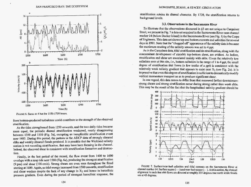
The connection between tidal motions and stratification can be more clearly seen in Figs. 4-6, a sequence of plots of top-bottom salinity difference and the square of the depth-averaged velocity (Figs. 4a to 6a), and of the streamwise velocity component for 3 depth cells, zl, z7, and 213, that are 3 m, 9 in, and 15 m above the bottom respectively (Fig. 4b to 6b). In these figures we have also marked periods in which the top-bottom shear is negative; it is during these times that shear should act to create stratification (see eq. 4). In all of these plots, it appears that negative shear is not sufficient for stratification to develop; instead low tidal energy, indicative of weak turbulent mixing, and negative shear are both important.

For example, the sequence of 5 diurnal stratification events that start at 1220 hours (Fig. 4a) all commence in periods when mixing is weak and shear is

16 2 a

-1

-2

1150 1200 1250 1300 1350

Time (h)

100 VI .. 6 Y x o v

.- - -100

1150 1200 1250 1300 1350

Time (h)

FIGURE 4. Conditions observed between 1150 and 1350 hours in Carquinez Strait: (a) Top-bottom salinity difference (- - -), depth-averaged velocity squared (-), and sign of top bottom shear (dots) - when shear is negative sign is set to 1, otherwise zero; (b) Velocities measured by ADCP 3 m, 9 m, and 15 m above the bed.

132

1350 1400 1450 1500 1550

Time (h) b

100 - m \

!3 Y x o v

.d " d

-100 I ' I I .

1350 1400 1450 1500 1550

Time (h)

FIGURE 5. Same as 4 but for 1350-1550 hours.

stabilizing. This coincides with alternate weak ebbs. Showing the importance of vertical mixing, the stratification disappears during each of the subsequent strong ebbs despite the fact that these ebbs could, via the SIPS mechanism, lead to stratification formation rather than destruction. This pattern in tidal mixing led to a predominantly diurnal stratification cycle. During this period of time there was little change in Q or in X2, hence all of the modulation in stratification was associated with variations in the barotropic tide.

Figure 4b shows the development of large tidally varying shears, mainly on the ebbs, with flood shears generally much weaker. This is what Jay & Musiak (1994a) would refer to as ebb-flood asymmetry. Even the weakest ebb shears offer considerable potential for producing stratification. If we assume an M2 varying sinusoidal shear with a peak value of 0.5 m/s and a longitudinal gradient of 0.4 psu/km, we can calculate that in the 6 hours starting at 1220 hours, tidal straining could create a salinity difference of about 3 psu, slightly less than the 4 psu observed. It seems likely that the difference here is the upper 3 m of the water column the ADCP does not see. This region could contain significant shear, and since it is hrther removed

133


stratification retains its diurnal character. By 1730, the stratification returns to background levels.

3.3. Observations in the Sacramento River To illustrate that the observations discussed in $3 are not unique to Carquinez

Strait, we present in Fig. 7 a data set acquired in the Sacramento River near channel marker 14 (below Decker Island) in the Sacramento River (see Fig. 1) by the Corps of Engineers. This data set shows top and bottom currents and salinities for several days in 1991. Note that the “chopped off’ appearance of the salinity data is because the maximum reading of the salinity sensors was set to 4 ppt.

As in the Carquinez data, tidal stratification and de-stratification, along with the concomitant development of sizeable top-bottom shear, are evident. As before, stratification and shear are associated mainly with ebbs. Given the relatively low salinities seen at this site, ie. , bottom salinities in the range of 1 to 4 ppt, the small degree of stratification that forms (a few tenths of a ppt) is consistent with the relatively weak salinity gradient that appears to exist near X2 (see Fig. 2a). It is impressive that even this degree ofstratification is sufficient to dramatically modify vertical momentum transport so as to produce significant shear.

In one regard, this data seems to differ from that measured farther downstream: strong shears and strong stratification occur during strong rather than weak ebbs. This may be the result of the fact that the longitudinal salinity gradient should be

Time (h)

200 ;

-200 .I 1650 1700 1750 1550 1600

Time (h)

FIGURE 6. Same as 4 but for 1550-1750 hours.

from bottom-produced turbulence could contribute to the strength of the observed stratification.

As the tides strengthened from 1250 onwards, and the two daily tides became more equal, the periodic diurnal stratification weakened, nearly disappearing between 1350 and 1550 (Fig. Sa), excepting an inexplicable stratification event near 1485. During this period, the pattern in the ADCP data of strongly sheared ebbs and weakly sheared floods persisted. It is possible that the Wickland salinity station is not recording stratification, that may have been forming in the channel. Indeed, the observed shear is consistent with stratification formation and destruction.

Finally, in the last period of the record, the flow event from 1400 to 1600 overlaps with a neap tide near 1580 (Fig. 6a), producing the strongest stratification (9 psu) and shear (100 c d s ) . Strong shears are even seen throughout the flood starting at 1600. Again, as tidal energy increased from 1580 onwards, stratification and shear weaken despite the lack of any change in X2 and hence in baroclinic pressure gradient. Even during the period of strongest baroclinic response, the

134

133 133.5 1 k Ih.5 135 1i5.5 1;6 Days

FIGURE 7. Surfacehear-bed salinities and tidal currents on the Sacramento River at channel marker 14. Surface sensor (-- -)and near-bed sensor (-). At this station, the channel alignment is such that ebb flows are directed at roughly 235 degrees true north while floods are at 45 degrees.

135


much stronger during the strong ebb at this location because salinities are higher at the end of flood, and hence so are horizontal salinity gradients.

3.4. Analysis of Carquinez ADCP data using Principal Components Analysis The dynamic nature of the vertical velocity shear is well illustrated through the

use of principle components analysis (PCA). PCA is a multivariate statistical method that separates a set of (observed) time series into a number of orthogonal (independent) spatial functions, or principle components, each of which has an associated amplitude, varying in time (see Kundu & Allen 1976; Walters & Gartner 1985). It has been widely used in oceanography to extract the behavior of different modes of motion or fluctuation from observations of currents, water levels, salinities, etc.

The relative importance of each of the principal components is expressed as a percent of the variance of the original data set explained by each component. The original data time series can be reconstructed by a linear combination of the amplitude of each principle component at that depth, multiplied by the appropriate temporally-varying amplitude. PCA is most useful when a physically relevant mode can be identified, since then it can be used to define the time behavior of that mode (Kundu & Allen’s 1976). Thus, as we will see below, the separation of baroclinic (gravitational circulation) and barotropic (tides) flows need not be defined by temporal filtering. As we will demonstrate below this is especially important when examining gravitational circulation, which appears to fluctuate in strength diurnally and semi-diurnally, and thus is not, strictly speaking, as is commonly assumed, a subtidal phenomenon.

To analyze ADCP data, complex PCA (Preisendorfer 1988) must be used: The horizontal velocity vector in a given bin is split into a real part, the streamwise velocity, U, and an imaginary part, the transverse velocity, V, i.e., we from the complex velocity Q as:

where z, is the velocity in the ith bin. The rest of the analysis proceeds as with a single set of time series, albeit with complex covariance matrices, rather than real ones, yielding complex structures for the principal components, i.e., structures that have both transverse and streamwise variability. Without detailing the specific mathematical manipulations, the result is that we write Q as:

Q(zi ,f) = U(z, ,f) + i V(zi ,f), (6)

m

Q (zi>t) = C Arn(t) 0 rn(zi> (7) m= 1

where A , the complex amplitude of the mth mode and 0,,,, the complex vertical structure function for the mth mode, are calculated from the n x n covariance matrix formed with Q.

The Carquinez Strait ADCP data set yielded suitable time series of velocity in 14 bins, accordingly, PCA gave 14 eigenfunctions (n = 14). According to the “scree” test which examines the way in which the variance explained depends on mode number (Preisendorfer 1988), the first three of these are statistically signifi-


*O L 15

- v ti 10 N

5

0

-0.5 0.0 0.5 1 .o 1.5 Velocity

FIGURE 8. Shapes of the first two principal components of ADCP velocity data froin Carquinez Strait, FebruarylMarch 1991: PCI ( ) U(z), (+) V(z); PC2 (*) U(z), (x ) V(z). U and V for PC2 have been offset by 0.75 units for clarity.

cant. The vertical structure of the first two principal components which result are displayed in Fig. 8. The first principal component, PC1 has the boundary-layer appearance one would expect for the barotropic tide and rotates a little with depth, presumably due to curvature in Carquinez Strait (Geyer 1993). The velocity shear seen in PCl is somewhat larger than would be expected for an homogeneous boundary layer, suggesting that this mode is influenced by stratification. Although it too turns with depth, the second principal component, PC2, has the classic profile of gravitational circulation, with two counterflowing layers. The first component accounts for 97.5% of the variance in the ADCP data while the second component accounts for nearly 80% of the remaining variance. Clearly, these two components define the flow,

The time dependence for PCI and PC2 are given in Fig. 9 where it can be seen that both modes oscillate semi-diurnally. A comparison of the time series of PCl amplitude with harmonic predictions made for nearby station C24 shows that the amplitude of PCl is predictable (a linear relation can be fit withR2 = 0.95) and thus that PCI is the barotropic tide.

While the vertical structure of PC2 appears to be that which would be expected for gravitational circulation, its time variation is different in that it fluctuates tidally rather than slowly responding to changes in longitudinal salinity gradient or tidal energy. However, confirming the fact that it accounts for the non-boundary-layer portion of the top-bottom shear, the low frequency variability of PC2 tracks that of AU = U(z13) - U(z1). This is illustrated in Fig. 10 where a 30 h moving-average smoothing has been applied to both these variables to remove tidal variations. The correspondence of the smoothed AU and PC2 time series offers strong support for

136 137


200 I I I I I MONISMITH, BURAU, & STACEY: CIRCULATION

,--. ? 100 5 - - 0 5 -- -100 3

I

I I I

Time (h)

I I 1800

-200 1 1400 1600 1000 1200

75 . I I

. . . . I I -50 1 I I 1800 1400 1600 1000 1200

Time (h)

I I I I I

I I I I

1800 -60

1400 1600 1000 1200 Time (h)

I I I

1600 1800 1200 1400 1000 Time (h)

FIGURE 9. Time series of PCI and PC2 amplitudes for ADCP data from Carquinez Strait, Februaryhlarch 1991: (a) PC~:u(zl~, t); (b) Pc~:V(zli, t); (c) PC~:U(ZI~, t); (d) PC2: v(zl3, t).

h

2 a v

0

-10

-20

-30

-40

-SO

h

v

. - - 1000 1100 1200 1300 1400 1500 1600 1700 1800

Time (h)

FIGURE 10. Subtidal behavior of: AS (x); U2(zli,t) multiplied by 1.92 to show correspondence to AU (+); and PC2 (-).

our interpretation of PC;, as a gravitational circulation mode. Most importantly, as we discussed in $1, the connection between AS, also smoothed to remove tidal variations, and PC2, is striking. When ASis large, PC2, i.e., gravitational circulation is strong; conversely, when AS is small, gravitational circulation is weak.

To examine how the barotropic and baroclinic flows behave at the tidal time scale, we focus separately on three periods during the flow: the first neap tide from hours 1 195- 1295 (neap I), the spring tide from hours 1370- I470 (spring) and the second neap tide from hours 1545- 1645 (neap 2). These are given as Fig. 1 I a, 1 1 b, and 1 Ic respectively.

Neap l(ll95-1295) During this period, the first principal component displays the strong diurnal

inequality that characterizes neap barotropic tides in this part of San Francisco Bay at this time of year. (Cheng & Gartner 1984) At the same time, the baroclinic flow consists of a series of “pulses” of exchange flows (in the streamwise direction only -the same pulsing does not appear in the cross-channel direction). PC2 tends to “turn on” for periods ranging from 1 or 2 hours to as many as 5 hours. During these pulses, the surface current is strongly down-estuary, at as much as 35 cmds, implying similarly intense up-estuary flows near the bottom. These pulses seem to extend from near the maximum ebb tide to just after the start of the flood tide.

In terms of SIPS, we would expect that when turbulent mixing is weak, a stratified water column will be produced during ebbs that then will destratify during the ensuing flood. The strong pulses of baroclinic flow which begin during the weak ebbs (at hours 1220, 1245, and 1270) thus should be coincident with stratification. During the strong ebb tides (at hours 1210, 1235, 1260, and 1285), the behavior of the baroclinic flow alters and displays a “double-pulse” behavior.

138 139


160

0

$ -160

m‘

h

--. v - Y

-320 v ...

-480

-640 1250 1275 1200 1225

Time (h) 75

50 0 c

m % 25 2 5 -160

160

- --.

c v v - 0 0 3 q -320 .. -. m

v) v

v 4

-25

-50

-480

-640 1400 1425 1450 1375

Time (h) 75

50

m N-

25 2 6 -160

160

0 c h --.

c v v h h

Y m 0 0 3 $ -320 .. VI v

v

-25 -480

-50 -640

1575 1600 1625 1550 Time (h)

FIGURE 11. (a) U(zl,,t) induced by PCI (---) and PC2 (-) during first neap tide in ADCP record; (b) U(zl3,t) induced by PC1 (---)and PC2 (-) during first spring tide in ADCP record; (c) U(zl3,t) induced by PCI (---)and PC2 (-) during second neap tide in ADCP record. Note that this neap tide followed a flow event of 1200 m3/s.

When the barotropic tide accelerates, the baroclinic flow turns on briefly, then turns off as the barotropic tide nears its maximum, and the water column becomes well-mixed.

During the ensuing barotropic deceleration, the baroclinic flow again turns on and continues to act until the following flood tide. Just as above, we can hypothesize that tidal straining of the density field plays an integral role in establishing this behavior. As the flow begins to ebb, tidal straining begins to stratify the water column; as in the weak ebb case, the resulting stratification allows the baroclinic exchange flow to develop. In this case, however, the flow continues to accelerate, producing increased mixing, until the stratification is broken down, thus shutting off the baroclinic flow. Turbulent mixing prevents stratification from forming through the maximum ebb. Then, during the deceleration, turbulent mixing decreases, and tidal straining again stratifies the water column, resulting in a reap- pearance of the baroclinic flow. The net result is the double-pulse behavior which is seen near hours 1210, 1235, 1260, and 1285.

Spring (1370-1470)

During the spring tide we show the tides have uniform strength on ebb and flood (about 13O/s) and there is no diurnal inequality evident (except slightly weak ebbs at hours 1370 and 1395). The result ofthis stronger, sustained barotropic forcing is a marked change in the behavior of the second principal component. Instead of sustained pulses ofbaroclinic flow, the time behavior ofthe exchange flow consists of a series of “spikes” (particularly after hour 1410 when the barotropic tide becomes truly symmetric). The spikes ofbaroclinic flow differ from the pulses seen during the neap tide both in timing and duration. While the baroclinic flow pulscs lasted several hours during the neap tide, during the spring tide they tend to appear and disappear in less than an hour. Further, the spikes tend to occur as the barotropic tide turns from ebb to flood, rather than just after the maximum ebb.

Again the interaction of the density stratification with turbulent mixing is central: During spring tides, energetic barotropic flows keep the water column from becoming significantly stratified and thus gravitational circulation remains weak. The observed positive and negative spiking of PC2 is the result of a difference in phase between different parts of the water column, largely due to the differential effects of bottom friction acting on a stratified water column (Monismith & Fong 1995).

Neap 2 (1545-1645) As during the first neap tide, PCI displays a strong diurnal inequality during the

second neap period. The time series ofthe PC2 is characterized by a series of pulses that are much stronger than those seen during the first neap. In fact, the strongest pulse (just after hour 1585) results in a surface velocity ofabout 50 c d s . A surface velocity of this magnitude would correspond to a bottom velocity of about 41 cmk, or a top-bottom velocity difference of 91 cids. Clearly, the effect of stratification that follows the freshwater flow event in this period has been to intensify and prolong the pulses of baroclinic flow.

This event emphasizes the nonlinearity inherent to SIPS: the strong pulse of

140 141


exchange flow near hour 1585 also acts to rapidly stratify the water column. Taking a value of 90 cm/s for the top-bottom velocity difference, and a typical horizontal salinity gradient of 0.5 p s m , the strong pulse of exchange flow at hour 1585 would stratify the water column at a rate of 1.6 psu/hr. The pulse lasted for several hours, resulting in a top-bottom salinity difference which was probably greater than 5 psu. In fact according to Fig. 6, the maximum stratification was approximately 8 psu at 1590 hours. The ensuing flood did not break down this stratification and the level of stratification at the beginning of the next ebb was not zero; thus the double pulse behavior seen in the first neap was replaced by a single pulse of longer duration. The increased intensity and persistence of the exchange flow is what leads to the strong shear evident even after low-pass filtering.

3.5. The Creation of Residual Gravitational Circulation The mean flow recorded by the ADCP is shown in Fig. 12 along with a cubic

fit to the mean flow described by the theoretical shape given (for example) in Prandle (1991) (Le., eq. 2) and calculated assuming that r = 0.46 psdkm, a net specific discharge of 0.3 m2/s, and a vertical eddy viscosity vt = 3.7 x 10-3 m2/s.

While the fit to theory appears good, both the discharge and nt were adjusted to give a best fit (the latter as in Lung & O’Connor 1984). The specific discharge is roughly twice as large as what would be calculated by dividing the average flowrate (300 m3/s) by the local width (2000 m). This is not too serious a discrepancy given that this purely Eulerian analysis doesn’t account for the inwards Stokes drift flow (Jay 1991), and even the Eulerian mean flow need not be distributed uniformly across the cross section (Fischer 1972).

However, the eddy viscosity appears to be roughly 10 times smaller than would

Velocity (m/s)

FIGURE 12. Time-averaged velocity profile measured by ADCP ( 0 ) in Carquinez Strait for February/March 1991 compared with theoretical profile for gravitational circulation (-).


3.0 8.0 ,

1000 1200 1400 1600 1800 Time(h)

8.0 , I 15

, I-

0.0 -5 1000 1200 1400 1600 1800

Time@)

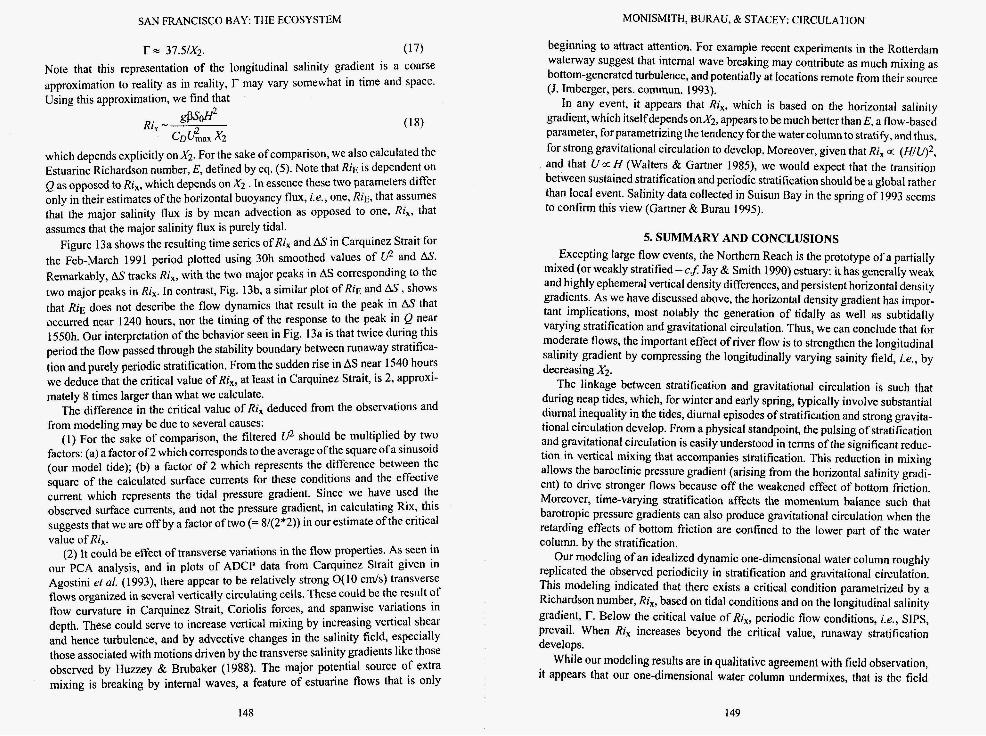
number, Ri, (----), and AS (-); (b) Estuarine Richardson number, RiE (---), and AS (-).

have been predicted using the standard formula for the depth-averaged viscosity (Prandle 1991) based on the fluid depth and on the rms tidal current. It is possible that this reduction is the averaged effect ofthe time-varying stratification, however, the stratification correction Uncles et al. (1990) used for modeling flows in the Tamar only gives a factor of two reduction in mixing rates when applied to this data set, leaving a substantial discrepancy.

Alternatively, the ADCP data itself makes the case that the gravitational flow

FIGURE 13. Time variations of stratification and stability parameters: (a) SIPS Richardson

142 143


is highly unsteady, behavior that is entirely consistent with the underlying physics. Thus, as we have seen above, variations in salinity stratification, vertical shear and gravitational circulation are all intertwined. Two key pieces of this puzzle are the stabilizing effect of stratification on turbulence and the creation and destruction of stratification by differential advection. The net effect is periodic stratification that is similar to but not quite identical to that which would be expected from the SIPS model advanced by Simpson and his colleagues. Accompanying this periodic stratification are periods of intense gravitational circulation. Looking at subtidal variability, when several strong stratification events occur sequentially, the concomitant gravitational circulation pulses appear as a sustained period of gravitational circulation.


4. MODELING STRATIFICATION DYNAMICS 4.1. Model Philosophy

To model the stratification response of the northern reach to flow and tide variations one can either proceed by applying a full three-dimensional hydrodynamic model (i.e., Casulli & Cheng 1992) or by simplifying the flow in some way. The flow to be calculated can be simplified by averaging over the width of the estuary; Ford et al. (1990) presented such model which they applied with some success to the northern reach.

A third alternative is one in which streamwise variations in all flow properties (excepting salinity) are eliminated and the dynamics of a complex three-dimensional estuary are reduced to that appropriate to a single hypothetical water column (Nunes-Vaz & Simpson 1994). This approach, which we pursue, represents a dynamic version of the steady state analytical theories that have traditionally been used to describe these flows.

4.2. The Model We used Blumberg et al. (1992)’s model, referred to hereafter as the BMY

model3, to calculate water column structure. Rather than use parametric representation of turbulent mixing processes like billowing, etc. (Monismith & Fong 1995), this model uses formal turbulence closure to obtain eddy mixing coefficients and so close the mean momentum and salt equations. As in other ID models (e.g., Simpson & Sharples 1992, Nunes-Vaz & Simpson 1994), the flow is assumed to be homogenous in both horizontal directions, thus eliminating gradients of every- thing except pressure and salinity in the x directions. If we neglect rotation, we have two equations for the two unknowns:

\ I To model SIPS, we have included streamwise advection of the salt field in the

’ This code was graciously provided to us by Dr. Alan Blumberg of Hydroqual, Inc.

144

salt balance using a value of r that is constant. In contrast, Sharples et al. ( I 994) found it necessary to use time and depth-dependent values of r to qualitatively reproduce stratification in the York River Estuary. The eddy mixing coefficients K,, and Ks are solved for using the Mellor-Yamada level 2.5 turbulence closure (Mellor & Yamada 1982) which defines them in terms of the turbulence length scale, L, and turbulence velocity scale, q, and two empirical constants, C,,, and C, as

( 9 4 (9b)

K, = C,qL Ks = C,qL

Two more transport equations must be solved for q and L; these are based on approximation of exact equations for transport of the Reynolds stresses.

The Mellor-Yamada level 2.5 closure is widely used in modeling coastal and estuarine flows; it is thought to be reasonably effective for describing effects of stratification on turbulence (Blumberg et al. 1992). However, in the form we use, there is an additional significant buoyancy modification. The master length scale L is subject to the stratification limit prescribed by Galperin et al. (1988):

& S 0.53

where N is the buoyancy frequency. This incorporates the well-known tendency of stratified turbulence to limit the vertical length scale ofturbulence to be no larger than the Ozmidov scale

L - - O - ( i 3 r

where e is the rate of turbulence \ / dissipation - q3/L (see Turner 1973).

The one-dimensional model requires that the pressure gradient be specified. While in principle this could be done using pressure gradients derived from a 2D circulation model like that described in Smith & Cheng (l987), we split the pressure gradient into two components. The first oscillates with period of 12 hours (approximately the M2 tide) and is the same as used by Monismith & Fong (1995). For reference sake this is:

\ / The second component, the baroclinic pressure gradient, drives gravitational

circulation; it is derived from the longitudinal salinity gradient. It has two components, one associated with the direct effect of the longitudinal salinity gradient, the other with the surface expression of the baroclinic pressure gradient. The combination of is:

145


where CD is the bottom drag coefficient. Note that in the Blumberg et al. (1 992) implementation of the Mellor-Yamada closure, CD is not specified, instead a bottom roughness zo is given. In general, CD depends on the height to which it is referenced. For example in our calculations if u* is related to the depth averaged tidal velocity, we find CD = 0.002.

The horizontal buoyancy flux that drives stratification formation is

Equating these two estimates (assuming a constant efficiency of conversion of TKE to potential energy - see Ivey & Imberger 1991) we expect that the non-dimensional stratification parameter

(17) Bstrat - gPrUmaxH2

where z = 0 is the bottom, z = H is the free surface. The free parameter a is used to adjust the tidally averaged flow in the model (Simpson & Sharples 1991).

The full set of equations are advanced in time using central differences in space and time, with a smoothing function used to eliminate temporal oscillations (see Blumberg & Mellor 1987). To model the Carquinez Strait data, we used a water column of 20 m discretized in 10 cm vertical increments. We found by experimen- tation that a time step of approximately 3 minutes was needed to give results that were independent of time step. The bottom roughness, ZO, which must be specified, was set to 1 cm. Adjustment of the flow to the given initial conditions were taken care of by allowing the flow to “spin-up” for one tidal cycle. This meant running the model so as to allow turbulence fields to develop and for the mean velocity profiles to adjust to the applied pressure gradients and mixing coefficient distribu- tions before we allowed the salt field to evolve. Once the flow was initialized, we ran the code to simulate 30 tidal cycles, or 15 days.

4.3. Model Results Initially (and rather naively), we chose U,,, = 0.75 m / s (although as seen in the

ADCP data it could easily be more during spring tides ) and r = 0.5 ppt/km. With these parameters specified we ran the code for different values of a. Depending on the choice of a, the water column went into one of three states: When a was set for a strong river flow, the water column would become completely fresh and the resulting flow would show a net outward flow superposed on the tidal oscillations. When a was set for a strong “negative” river flow (salt water moving upstream), the water column would become completely saline (match the ocean salinity). The third state, one of zero net flow, a condition that must be determined by repeatedly running the model, was a completely stratified regime, with completely fresh water flowing out at the surface and ocean water flowing in at the bottom. Apparently, the tidally-produced mixing energy was not sufficient to break down the stratification induced by the baroclinic motions.

However, by repeatedly running the model with different values of Urn,, , r, and H, it became evident that it was possible for the tidally produced turbulent mixing to balance the stratifying effects of and create periodic stratification. Empirically we found that boundary between periodic stratification and the “two- layer” estuary was determined by the expression

which has a simple physical interpretation: At the threshold velocity, we expect that the tidal generation of turbulent kinetic energy (TKE), say &ides, exactly balances the buoyancy flux, Bstrat, associated with the stratifying effects of baroclinic forcing (Abraham 1988):

u,,, = 0.12Hr”2 (14)

Etides - &rat (15)

The rate of creation of turbulent kinetic energy (TKE) by the barotropic tides will vary as:

Etides - cD&ax (16)

determines the boundary between flow states. Using our model runs, and assuming that CD = 0.002, we find a critical value ofRix = 0.25. When Ri, is greater than this O(1) constant, tidal energy is not sufficient to overcome the stratifying effects of baroclinic pressure gradients, tidal straining and frictional shears; accordingly, the water column will stratify. On the other hand, when it is subcritical, our model predicts that tidal mixing will be able to eliminate stntification caused by tidal straining and by the baroclinically forced mean flow.

4.4. Comparison of Model Results to Observations The model runs and scaling analysis we discuss above suggest that during

particularly strong tides, tidally produced turbulence should be able to overcome the stratifying effects of longitudinal variations in density and weak periodic stratification should appear. Conversely, when the tides are “weak” (in the sense defined by eq. 18 ), the tendency to create stratification will win out, possibly creating stratification that is not broken down during flood tides, and thus which strengthens during successive ebbs.

In our idealized model, this is the route to a “river-over-ocean” estuary. In reality, this scenario is not completed for several reasons:

( I ) r is a function of mean salinity (see Fig. 2a) -hence the assumption that r is does not depend on position in the water column or on time breaks down;

(2) We omit the effects of cross-sectional, i.e., shoal-channel, variability that could provide, in effect, additional vertical mixing (Huzzey & Brubaker 1988);

(3) More generally, dispersion due to horizontal variability of tidal currents (Zimmerman 1986; Fischer et al. 1979) will also tend to act to maintain salinities at intermediate values- i.e., the ID model can not represent the full salt balance that determines r.

Nonetheless, we can hypothesize that Ri, is a good parameter for delineating stratification behavior. We tested this hypothesis using the 1991 Carquinez Strait field data discussed in $3. We first interpolated the salinity, velocity, flow and& data to a common timebase with 1 hour increments. X2 is required in order to calculate Rix as a function of time since using figure 2b,

146 147


beginning to attract attention. For example recent experiments in the Rotterdam waterway suggest that internal wave breaking may contribute as much mixing as bottom-generated turbulence, and potentially at locations remote from their source (J. Imberger, pers. commun. 1993).

In any event, it appears that Ri,, which is based on the horizontal salinity gradient, which itselfdepends on&, appears to be much better than E, a flow-based parameter, for parametrizing the tendency for the water column to stratify, and thus, for strong gravitational circulation to develop. Moreover, given that Ri, oz ( H / Q 2 , and that U a H (Walters & Gartner 1985), we would expect that the transition between sustained stratification and periodic stratification should be a global rather than local event. Salinity data collected in Suisun Bay in the spring of 1993 seems to confirm this view (Gartner & Burau 1995).

I-0 37.5/X2. (17)

Note that this representation of the longitudinal salinity gradient is a coarse approximation to reality as in reality, may vary somewhat in time and space. Using this approximation, we find that

Ri, - gPS0H2 (18) C D U L x2

which depends explicitly on&. For the sake of comparison, we also calculated the Estuarine Richardson number, E, defined by eq. (5). Note that RiE is dependent on Q as opposed to Ri,, which depends on X2 . In essence these two parameters differ only in their estimates of the horizontal buoyancy flux, i .e., one, RiE, that assumes that the major salinity flux is by mean advection as opposed to one, Ri,, that assumes that the major salinity flux is purely tidal.

Figure 13a shows the resulting time series ofRi, and AS in Carquinez Strait for the Feb-March 1991 period plotted using 30h smoothed values of U2 and AS. Remarkably, AS tracks Ri,, with the two major peaks in AS corresponding to the two major peaks in Ri,. In contrast, Fig. 13b, a similar plot of RiE and A S , shows that R ~ E does not describe the flow dynamics that result in the peak in AS that occurred near 1240 hours, nor the timing of the response to the peak in Q near 1550h. Our interpretation ofthe behavior seen in Fig. 13a is that twice during this period the flow passed through the stability boundary between runaway stratification and purely periodic stratification. From the sudden rise in AS near 1540 hours we deduce that the critical value of Ri,, at least in Carquinez Strait, is 2, approximately 8 times larger than what we calculate.

The difference in the critical value of Ri, deduced from the observations and from modeling may be due to several causes:

( I ) For the sake of comparison, the filtered U2 should be multiplied by two factors: (a) a factor of 2 which corresponds to the average ofthe square of a sinusoid (our model tide); (b) a factor of 2 which represents the difference between the square of the calculated surface currents for these conditions and the effective current which represents the tidal pressure gradient. Since we have used the observed surface currents, and not the pressure gradient, in calculating Rix, this suggests that we are off by a factor of two (= 8/(2*2)) in our estimate of the critical value of Ri,.

(2) It could be effect of transverse variations in the flow properties. AS seen in our PCA analysis, and in plots of ADCP data from Carquinez Strait given in Agostini et al. (1993), there appear to be relatively strong O( 10 c d s ) transverse flows organized in several vertically circulating cells. These could be the result of flow curvature in Carquinez Strait, Coriolis forces, and spanwise variations in depth. These could serve to increase vertical mixing by increasing vertical shear and hence turbulence, and by advective changes in the salinity field, especially those associated with motions driven by the transverse salinity gradients like those observed by Huzzey & Brubaker (1988). The major potential source of extra mixing is breaking by internal waves, a feature of estuarine flows that is only

5. SUMMARY AND CONCLUSIONS Excepting large flow events, the Northern Reach is the prototype of a partially

mixed (or weakly stratified - c$ Jay & Smith 1990) estuary: it has generally weak and highly ephemeral vertical density differences, and persistent horizontal density gradients. As we have discussed above, the horizontal density gradient has important implications, most notably the generation of tidally as well as subtidally varying stratification and gravitational circulation. Thus, we can conclude that for moderate flows, the important effect of river flow is to strengthen the longitudinal salinity gradient by compressing the longitudinally varying sainity field, i .e., by decreasing Xz.

The linkage between stratification and gravitational circulation is such that during neap tides, which, for winter and early spring, typically involve substantial diurnal inequality in the tides, diurnal episodes of stratification and strong gravitational circulation develop. From a physical standpoint, the pulsing of stratification and gravitational circulation is easily understood in terms of the significant reduction in vertical mixing that accompanies stratification. This reduction in mixing allows the baroclinic pressure gradient (arising from the horizontal salinity gradient) to drive stronger flows because off the weakened effect of bottom friction. Moreover, time-varying stratification affects the momentum balance such that barotropic pressure gradients can also produce gravitational circulation when the retarding effects of bottom friction are confined to the lower part of the water column. by the stratification.

Our modeling of an idealized dynamic one-dimensional water column roughly replicated the observed periodicity in stratification and gravitational circulation. This modeling indicated that there exists a critical condition parametrized by a Richardson number, Ri,, based on tidal conditions and on the longitudinal salinity gradient, r. Below the critical value of Ri,, periodic flow conditions, i .e., SIPS, prevail. When Ri, increases beyond the critical value, runaway stratification develops.

While our modeling results are in qualitative agreement with field observation, it appears that our one-dimensional water column undermixes, that is the field

148 149


seems to be more strongly mixed than our model would lead us to expect. This could be the result of ignoring the mixing effects of internal waves, or, given that turbulence closures like that which we use tend to overmix, it the most likely source of the discrepancy arises through our neglect oftransverse flow variations like those observed by Huzzey & Brubaker (1988) or Simpson & Turrell(1986).

This mismatch of observations and modeling is not new. In their original modelingofLiverpool Bay, Simpson & Sharples (1991) were forced to use stronger currents in their model than they had observed in order to reproduce observed salinity stratifications. Applying several turbulence closures of varying sophistica- tion and finding results that depended on the closure used, Nunes-Vaz & Siinpson (1994) make the case that SIPS provides a tough test for any turbulence modeling. Thus, if three-dimensional hydrodynamic models of the type described by Casulli and Cheng (1992) are to be employed with any predictive skill in northcrn San Francisco Bay, it seems likely that turbulence models capable of accurately representing the effects of stratification on vertical mixing will be required.

What are the implications of the behavior discussed above for the transport of sediment or organisms? Given that sediment concentrations, for example, fluctuate tidally, it is conceivable that the actual rate of sediment transport is very much different from what one would calculate using mean velocities and mean concentrations. For example, if sediment concentrations were in phase with tidal currents, i.e., peak concentrations occur at or near peak velocities, little sediment would be transported in the fashion that is assumed to maintain the ETM, since gravitational crrculation and sediment concentrations would be nearly out of phase.

More generally, if we attempt to postulate circulation patterns that might exchange fluid particles (or organisms) between the shoals and channels of the Northern Reach, we must bear in mind the fact that the gravitational circulation pattern might only be operating for a part of the tidal cycle. One can imagine that a parcel of water leaving the shoals might be carried into a stratified, ebbing water column in the channel, and thus be transported relatively far downstream during the gravitational circulation pulse. At the end of the stratified period, this parcel of water would be mixed with salty water flowing landward underneath it. Regions of the shoals that exchanged fluid in this manner might be expected to have shorter residence times than those for which water parcels entered the channel during phases of the tide when the water column in the channel is not stratified.

Finally, when thinking about any process that depends on rates of vertical mixing, it is important to consider tidal and subtidal variabiliq of stratification. Unlike the simple models of decaying stratification considered in Koseff et a/. (1993), it may be necessary to consider a SIPS state as the basic flow configuration for, e.g. , phytoplankton modeling (J. Koseff, pers. commun. 1995).

ACKNOWLEDGEMENTS This work was supported by the EPA San Francisco Estuary Project and by the

Interagency Ecological Studies Program. We acknowledge the support provided by NSF through grant CTS-89583 14 to SGM and support from the US Geological

Survey to JRB. We also recognize the generous gift of computer equipment from Silicon Graphics. George Nichol of the Corps of Engineers provided the Sacra- mento River data at channel marker 14. The authors thank Ralph Cheng, Jeff Gartner, Pete Smith and Jeffrey Koseff for their help and advice. Finally, SGM thanks Vincenzo Casulli for hosting him in excellent style in Trento, Italy while he finished this paper.

REFERENCES Abraham, G. ( I 988). Turbulence and mixing in stratified tidal flow. Pagcs 149- 180 i n J.

Dronkers and W. van Leussen, eds., Physical Processes in Estuaria. Springer-Verlag., New York, NY.

Agostini, D., J. Evans, F. Wen, and P. Smith. (1993). Visualization and analysis of multi-dimensional velocity measurements in Carquinez Strait, California. Pages 1096- llOlin H. W. Shen, S. T. Su, & F. Wen, eds., Hydraulic Engineering '93, vol. 2. American SOC. Civil Eng., New York, NY.

Armor, C. A., and P. L. Herrgesell. (1985). Distribution and abundance of fishes in the San Francisco Bay Estuary between 1980 and 1982. Pages 21 1-227 in J. E. Cloern & F. H. Nichols, eds., Temporal Dynamics ofan Estuary: San Francrsco Bay. Junkers, Hingam, MA.

Arthur, J. F., and M. D. Ball. (1979). Factors influencing the entrapment of suspended material in the San Francisco Bay Estuary. Pages 143-174 in T. J. Conomos, ed., San Francisco Buy. The Urbanized Estuary. Pacific Division, American Association for the Advancement of Science, San Francisco, CA.

Blumberg, A. F., B. Galperin, and D. J. O'Connor. (1992). Modeling vertical structure of open channel flows .lour. Hydrol. Div.. American SOC. Civil Eng. 118: 1 119-1 134.

Blumberg, A. F., and G. L. Mellor. (1987). A description of a three-dimensional coastal ocean circulation model. Pages 1-16 in N. S. Heaps, ed., Three Dimensional Coastal Ocean Models. American Geophysical Union, Washington, DC.

Burau, J. R., M. R. Simpson, and R. T. Cheng. (1993). Tidal and Residual Currents Measured by an Acoustic Doppler Current Profiler at the West End of Carquiiiez Strait. San Francisco Bay, Calfornia, March to November 1988. US. Geol. SUN. Water Resour. Inv. Rept. 92-4064. 76 pp.

Casulli, V., and R. T. Cheng. (1 992). Semi-implicit finite difference methods for three-dimensional shallow water flow. lnternat Jour. Num. Methods in Fluids 15:629-648

Cheng, R. T., and J. W. Gartner. (1 984). Tides, tidaland residual currents in San Fr-anci.sco Bay, Cali$ornia- Resultsofmeasurements. Part 1 . U.S. Geol. SUN. Water Resour. Inv. Rept. 84-4339.72 pp.

Cloern, J. E. (1982). Does benthos control phytoplankton biomass in south San Francisco Bay? Marine Ecol. Progr. Ser. 9:191-202.

Cloern, J. E. (1991). Tidal stirring and phytoplankton bloom dynamics in an estuary. Jour. Marine Res. 49:203-221.

Conomos, T. J. (1979). Properties and circulation of San Francisco Bay waters. Pagcs 143-174 in T. J. Conomos, ed., San Francisco Bay: The Urbanized Estuary. Pacific Division, American Association for the Advancement of Science, San Francisco, CA.

Denton, R. A., and J. R. Hunt. (1986). Currents in San Francisco Bay-Final Report. Hydrol. and Coastal Eng., Dept. Civil Eng., Univ. California, Berkeley. Tech. Rept.

Fischer, H. B. (1972). Mass transport mechanisms in partially stratified estuaries. Jour. Fluid. Mech. 53:671-687.

Fischer, H. B., E. J. List, J. Imberger, R. C. Y. Koh, and N. H. Brooks. (1979). Mixing in Inland and Coastal Waters. Academic Press, New York, NY. 483 pp.

UCB/HEL-86/0 1.

150 151


Ford, M., J. Wang, and R. T. Cheng. (1990). Predicting thevertical structure of tidal current and salinity in San Francisco Bay, California. Wafer Resour. Res.26: 1027-1045

Galperin, B., and L. H. Kantha, S. Hassid, and A. Rosati. (1988). A quasi-equilibrium turbulent energy model for geophysical flows. Jour. Atmos. Sci. 4555-62.

Gartner J. W., M. R. Simpson, and R. N. Oltmann. (1995). Velocity Measurernerzts by Acoustic Doppler Current Profiler and Conventional Current Meters in Suisun Bay, San Pablo Bay, and Carquinez Strait, California, 1990-1991. U.S. Geol. Surv. Water Resour. Inv. Rept. (in press)

Gartner J. W. and J. R. Burau. (1995). Report offield measurements during a salt balance study an Suisun Bay, California, 1992-1993. U S . Geol. Surv. Water Resour. Inv. Rept. (in press)

Geyer, W. R. (1993a). Three-dimensional tidal flow around headlands. Jour. Geophys. Res. (Oceans) 98:955-966.

Geyer, W. R. (1993b). The importance of suppression of turbulence by stratification on the estuarine turbidity maximurn. Estuaries 16:113-125.

Hanscn. D. V.. and M. Rattray, Jr. (1966). New dimensions in estuary classification. Lirnnoi.


Oceanogr. 11.3 19-326. Herbold, B., A. D. Jassby, and P. B. Moyle. (1992). Status and Trends Report on Aquatrc

Resources in the San Francisco Estuary. Report to the EPA San Francisco Estuary Project. 257 pp.

Huzzey, L. M. and J. M. Brubaker. (1988). The formation of longitudinal fronts in a coastal plain estuary. Jour. Geophys. Res. (Oceans) 93: 1329-1 334.

hey, G. N. and J. Imberger. (1991). On the nature of turbulence in a stratified fluid. Part 1 : The energetics of mixing. Jour. Phys. Oceanogr. 2 1:650-658.

Jassby, A. D., W. M. Kimmerer, S. G. Monismith, C. Armor, J. E. Cloern, T. M. Powell, J. Schubel, and T. Vendlinski. (1995). Isohaline position as a habitat indicator for estuarine resources: San Francisco Bay-Delta, California, U.S.A. Eco1,Applications. 5:272-289.

Jassby, A. D., J. R. Koseff, and S. G. Monismith. (1995 [1996]). Processes underlying phytoplankton variability in San Francisco Bay. Pages 325-349 in T. Hollibaugh, ed., Son Francisco Bay: The Ecosystem. Pacific Division, American Association for the Advancement of Science, San Francisco, CA.

Jav. D. A. (1991). Estuarine salt conservation: A Lagrangian approach. Estuarine Coastal ShelfSci. 32547-565.

Jay, D. A,, and J. D. Musiak. (1995a). Internal tidal symmetry in channel flows: Origins and consequences. In: C. Pattiaratchi, ed., Mixing Processes in Estuaries and Coastal Seas. American Geophys. Union. (in press).

Jav. D. A.. and J. D. Musiak. (1995b). Particle trapping in estuarine tidal flows. Jour. - ,I

Geophys. Res. (Oceans) (in press). Jay, D. A,, and J. D. Smith. (1990). Residual circulation in shallow estuaries 2.Weakly

stratified and Dartially mixed, narrow estuaries. Jour. Geophys. Res. (Oceans) 95(cl): 713-748.

Kimmerer, W. M. (1992). An Evaluation of Existing Data in the Entrapment Zone of the San Francisco Bay Estuary. Interagency Ecol. Studies Program for the Sacramento-San Joaquin Estuary Tech. Rept. 33.49 pp.

Koseff, J. R., J. K. Holen, S. G.Monismith, and J. E. Cloern. (1993). The effects of vertical mixing and benthic grazing on phytoplankton populations in shallow turbid estuaries. Jour. Marine Res. 5 i:1-26:

quency current fluctuations near the Oregon coast. Jour. Phys. Oceanogr. 6: 18 1-199. Kundu, P. K., and J. S. Allen. (1976). Some three-dimensional characteristics of low-fre-

Lung, W. S., and D. J. O'Connor. (1984). Two-dimensional mass transport in estuaries. Jour. Hydrol. Eng. 110:1340-1357.

geophysical fluid problems. Rev. Geophys. Space Phys. 20:85 1-875. Mellor, G. L., and T. Yamada. (1982). Development of a turbulence closure model for

Monismith, S. G, and Fong, D. A. (1995). A simple model of mixing in stratified tidal flows. Jour. Geophys. Res. (Oceans) (in press).

Nunes Vaz R. A. and G. W. Lennon. (1991). Modulation ofestuarine stratification and mass flux at tidal frequencies. Pages 505-520 in B. B. Parker, ed., Tidal Hvdrodynamics. Wiley Interscience, New York, NY.

Nunes Vaz R. A. and J. R. Simpson. (1994). Turbulence closure modeling of estuarine stratification. Jour. Geophys. Res. (Oceans) 99:16143-16160.

Nunes Vaz, R. A., G. W. Lennon and J. R. de Silva Samarasinghe. (1989). The negative role of turbulence in estuarine mass transport. Estuarine Coastal ShelfSci. 28:36 1-377.

Prandle, D. ( I 985). On salinity regimes and the vertical structure ofresidual flows in narrow tidal estuaries. Estuarine Coastal ShelfSci. 20:6 15-635.

Prandle, D. (1991). Tides in estuaries and embayments (review). Pages 125-152 in B. B. Parker, ed., Tidal Hydrodynamics. Wiley Interscience, New York, NY.

Preisendorfer, R. W. (1 988). Principal Component Analysis in Meteorology and Oceanog- raphy. Elsevier, New York, NY. 425 pp.

Schubel, J. R. (1968). Turbiditymaximum ofnorthem ChesapeakeBay. Science 161:1013- 1015.

Sharples, J., J. H. Simpson, and J. M. Brubaker. (1994). Observations and modelling of periodic stratification in the Upper York River Estuary, Virginia. Estuarine Coastal ShelfSci. 3 8:30 1 -3 1 2.

Simpson, J. H., and J. Sharples. (1991). Dynamically-active models in the prediction of estuarine stratification. Pages 101-1 13 in D. Prandle, ed., Dynamics and Exchanges in Estuaries and the Coastal Zone. Springer-Verlag, New York, NY.

Simpson J. H., J. Brown, J. Matthews, and G. Allen. (1990). Tidal straining,density currents, and stirring in the control of estuarine stratification. Estuaries 13:125-132.

Simpson, J. H., and W. R. Turrell. (1986). Convergent fronts in the circulation of tidal estuaries. Pages 139-152 in D. A. Wolfe, ed., Estuarine Variability. Academic Press, New York, NY.

Smith L. H., and R. T. Cheng. (1987). Tidal and tidally averaged circulation characteristics of Suisun Bay, California. Water Resour. Res. 23:143-155.

Smith, P. E., R. T. Cheng, J. R. Burau, and M. R. Simpson. (1991). Gravitational circulation in a tidal strait. Pages 429-434 in R. M. Shane, ed., Hydraulic Engineering 1991. American SOC. Civil Eng., New York, NY.

Turner, J. S. (1973). Buoyancy Effects in Fluids. Cambridge Univ. Press, Cambridge, UK. 368 pp.

Uncles, R. J., J. A. Stephens, and M. L. Barton. (1991). Observations of fine-sediment concentrations and transport in the turbidity maximum region of an estuary. Pages 10 1 - 1 13 in D. Prandle, ed., Dynamics and Exchanges in Estuaries and the Coastal Zone. Springer Verlag, New York, NY.

Vidergar, L. L., J. R. Koseff, and S. G. Monismith. (1993). Numerical models of phytoplankton dynamics for shallow estuaries. Pages 1628-1634 in H. W. Shen, S. T. Su, & F. Wen, eds., Hydraulic Engineering '93, vol. 2. American SOC. Civil Eng., New York, NY.

Walters R. A., and J. W. Gartner. (1985). Subtidal sea level and current variations In the northern reach of San Francisco Bay. Estuarine Coast. ShelfSci. 2 1: 17-32.

Zimmerman, J. T. F. (1986). The tidal whirlpool: A review of horizontal dispersion by tidal and residual currents. Netherlands Jour. Sea Res. 20: 133-154.

152 153

SAN FRANCISCO BAY AND ENVIRONS This is a portion of a NASA Landsat Thematic Mapper digital image recorded on

June 20, 1990 from an altitude of approximately 675 km. (Color infrared composite of bands 4,3, and 1; contrast sketched; scene identifier 52302-18061, pathhow 44-34.)

Each pixel has a resolution of approximately 30 m. Image provided courtesy of William Acevedo of NASA and Richard Smith of the U.S. Geological Survey.

I

SEVENTY-FIFTH ANNUAL MEETING of the PACIFIC DIVISION/AMERICAN ASSOCIATION FOR THE ADVANCEMENT OF SCIENCE

I held at SAN FRANCISCO STATE UNIVERSITY, SAN FRANCISCO, CALIFORNIA June 19-24, 1994


With Reference to the Influence of Man Further Investigations into the Natural History of San Francisco Bay and Del

__

Ita

Editor James T. Hollibaugh

Romberg Tiburon Center San Francisco State University

San Francisco, Calqomia 1996

STRATIFICATION DYNAMICS AND GRAVITATIONAL … burau, & stacey: circulation stratification dynamics...

Documents

Transcript of STRATIFICATION DYNAMICS AND GRAVITATIONAL … burau, & stacey: circulation stratification dynamics...