
Strategy Meets Evolution: Games Suppliers and Producers Play
26
STRATEGY MEETS EVOLUTION : GAMES SUPPLIERS AND PRODUCERS PLAY Brishti Guha 1 Singapore Management University Abstract Final goods producers, who may be intrinsically honest (a behavioral type) or opportunistic (strategic), play a repeated game of imperfect information with suppliers of an input of variable (and non-verifiable) quality. Returns to cheating are increasing in the proportion of intrinsically honest producers. If producers compete for another scarce input, adverse selection reduces this proportion enough to enforce universal honesty, whether at a high or a low quality equilibrium. This mechanism limits the proportion of behavioral types in the population of producers over a wide range of parameters: despite their inability to compete with opportunists, they are not wholly wiped out due to the strategic response of input suppliers. Moreover, in equilibrium, opportunists must replicate the behavioral type’s behavior. Thus competition curtails the presence of the behavioral type but increases the incidence if its behavior. If a labor market, where skilled and unskilled labor coexist, is also endogenized, an honest equilibrium with both high and low quality will generally be reached; however an exclusively high quality equilibrium with unemployment of unskilled labor is also possible. JEL Classification : C7, D8, J4. Keywords: Moral hazard, evolution, strategic response, repeated games, skill. 1 The School of Economics and Social Sciences, Singapore Management University, 90 Stamford Road, Singapore 178903. I began work on this paper while at the Department of Economics, Princeton University. I would like to acknowledge helpful input from Ashok Guha. 1
Transcript of Strategy Meets Evolution: Games Suppliers and Producers Play
STRATEGY MEETS EVOLUTION :
GAMES SUPPLIERS AND PRODUCERS PLAY
Brishti Guha1
Singapore Management University
Abstract
Final goods producers, who may be intrinsically honest (a behavioral type) or
opportunistic (strategic), play a repeated game of imperfect information with suppliers of
an input of variable (and non-verifiable) quality. Returns to cheating are increasing in
the proportion of intrinsically honest producers. If producers compete for another scarce
input, adverse selection reduces this proportion enough to enforce universal honesty,
whether at a high or a low quality equilibrium. This mechanism limits the proportion of
behavioral types in the population of producers over a wide range of parameters: despite
their inability to compete with opportunists, they are not wholly wiped out due to the
strategic response of input suppliers. Moreover, in equilibrium, opportunists must
replicate the behavioral type’s behavior. Thus competition curtails the presence of the
behavioral type but increases the incidence if its behavior. If a labor market, where
skilled and unskilled labor coexist, is also endogenized, an honest equilibrium with both
high and low quality will generally be reached; however an exclusively high quality
equilibrium with unemployment of unskilled labor is also possible.
JEL Classification : C7, D8, J4.
Keywords: Moral hazard, evolution, strategic response, repeated games, skill.
1The School of Economics and Social Sciences, Singapore Management University, 90 Stamford Road, Singapore 178903. I began work on this paper while at the Department of Economics, Princeton University. I would like to acknowledge helpful input from Ashok Guha.
1

1. Introduction
Recent theory has been divided on the merits of continuing to assume that all
economic agents are perfectly rational, where rationality is defined as following fully
optimizing behavior. Accordingly, there has been no dearth of studies modeling some
form of bounded rationality. In particular, two main alternatives to “strategic” or “fully
optimizing” behavior were developed – evolutionary game theory and adaptive
heuristics. In the former, agents follow a fixed “outcome-independent” strategy :
different proportions of agents in the population follow different strategies and evolution
“selects” the best strategy – or set of strategies - over time, subject to “mutations” –
random changes or transitions in the strategy followed. In the latter, agents are not
perfectly rational but may use a simple rule (for example, one based on regret matching –
see Hart (2005)) to determine whether to switch to an alternative strategy.
Our paper attempts to fill a gap in this literature by focusing on the interaction
between strategic optimizing types and types following a behavioral rule, when both
types belong to a class of agents playing a repeated game against agents of another class
(who, for simplicity, are all assumed to be rational). We apply our analysis to a problem
of moral hazard between input suppliers, who supply inputs of variable but non-verifiable
quality to final goods producers. Transfer prices for the inputs may be determined
through Nash bargaining, however, final producers have the option to cheat their
suppliers by falsely claiming that the input they had been supplied was of low quality,
thus paying a low price for a high-quality input. The population of final producers is
heterogeneous, with some intrinsically honest agents who always stick to honesty
irrespective of economic considerations, and some opportunistic producers who are
standard optimizing agents. Matching is the result of a search process, but once a match
is formed it can persist into future periods unless it is terminated either exogenously or
deliberately. We describe possible equilibria in three different models. All the models
have the common feature that suppliers can supply inputs of high quality (using skilled
labor at a wage ws) or low quality (using unskilled labor at a wage wu) to heterogeneous
producers (either intrinsically honest or opportunistic) who transform these inputs into
high or low quality products respectively which sell at prices PH and PL.
2
In our first model, we have exogenous wages and final prices, implying perfectly
elastic supply of all primary factors and perfectly elastic demand for all final products, as
in a small open economy (so that there is no competition between producers in the factor
or product markets).
In the second, wages and final prices are still exogenous, but production requires
an additional factor, working capital, which is in inelastic supply and for which producers
have to compete. The element of competition introduces the interaction between strategic
and behavioral agents, both of whom are playing against agents of another class.
Interestingly this mechanism serves to limit the proportion of behavioral types in the
population for a wide range of parameters. The behavioral types’ strategy is inferior, in
the relevant parameter space, and this leads to their downfall : however, the type is not
entirely wiped out, and this is due to the strategic response of input suppliers – the other
class of agents. What is more, in contrast to the first model, equilibria in this model
necessarily involve honesty – whether high or low quality is being supplied. Thus,
although the proportion of the behavioral type in the population goes down, their strategy
is now followed by every one. We therefore have a situation where, although “survival
of the fittest” operates, the strategies followed by the unfit may prevail in equilibrium,
due to the strategic interaction with other agents (input suppliers). Incorporation of the
channel of competition between producers changes behavior in equilibrium, and also
rules out multiple equilibria obtaining for the same parameter ranges that characterized
the first model – serving as an equilibrium selection device for the relevant range of
parameters.
In our third model, wages are endogenously determined by labor demand and
inelastic supplies of each labor skill, though final product prices remain exogenous (as
they would be in a small open economy). In general, we can show that a single
equilibrium obtains here where both high and low quality co-exist – with workers of both
skill levels being employed – but in some circumstances (if exogenous separations of
matches are very frequent, and agents are impatient) we may have an equilibrium in
which there is involuntary unemployment of unskilled labor, with only high quality being
supplied and produced in equilibrium.
3

Our paper thus relates to two of the three approaches in modeling agent behavior
mentioned above – fully optimizing behavior and a behavioral genotype. We do not deal
with adaptive heuristics. One strand of the related literature encompasses models of
repeated moral hazard between fully optimizing players. This is an extensive literature
and the ideas underlying it date at least as far back as Williamson (1979) and Grossman
and Hart (1986). One or two-sided prisoner’s dilemma models with scope for cheating
include those by Diamond (1991), Dixit (2003) and Greif (1993). Often, prisoner’s
dilemmas in large populations exhibit i.i.d random matching in such papers, in contrast to
our approach of allowing for persistent relationships, though a relationship may be
terminated either deliberately or due to exogenous reasons. Papers such as Gul (2001)
analyze hold-up problems and bargaining in a buyer-seller context, and this is also related
to our model.
Some papers (eg Dixit 2003) also contain some behavioral players in a two-sided
prisoner’s dilemma. However, there is no mechanism whereby the optimizing and the
behavioral players belonging to the same class of agents compete : as such the second
model in our paper, by introducing such a mechanism, lends itself to an evolutionary
interpretation – the force behind selection being an economic one. This brings us to
another relevant strand of literature, that on evolutionary game theory. Unlike standard
evolutionary models we emphasize the effect of strategic or optimizing agents on
behavioral types and on strategies that survive in a population. Moreover, the
mechanisms embedded in our second model as well as in our third model (which enables
us to characterize conditions in the labor market in a general equilibrium setting and to
predict in what circumstances involuntary unemployment of unskilled labor may emerge)
serve as equilibrium selection devices eliminating the possibility of multiple equilibria
for the same parameter values. So this links our work to the literature on equilibrium
selection (which includes Myerson (2004 ) ).
2. Model I : Perfectly Elastic Factor Supplies
2.1 Assumptions We assume that suppliers can supply inputs of high quality (using skilled labor at
a wage ws) or low quality (using unskilled labor at a wage wu) to heterogeneous
4

producers (either intrinsically honest or opportunistic) who transform these inputs into
high or low quality products respectively which sell at prices PH and PL .
For the purposes of this first model, wages of both types of labor are exogenously
fixed, all inputs are in perfectly elastic supply and hence there is no competition between
producers in the factor market. Throughout we assume that final good prices are
exogenous as in a small open economy. Moreover parameters are such that PH- ws> PL -
wu so that the total surplus (to be shared among each matched supplier and producer)
from high quality production is never lower than that associated with low quality
production.
There are M suppliers and N producers where M and N are large numbers and
M<N. Of the N producers, a proportion α is intrinsically honest.
Each period one supplier can be matched with only one producer, and vice versa.
Matching involves search by suppliers and producers who are on the market for new
matches : however those whose previous match has not been either deliberately or
exogenously terminated remain in the old relationship and do not enter the market. A
fraction 1-γ of all matches terminate exogenously (so that 1-γ is the probability of
exogenous separation).
Our assumption regarding informational structure throughout is that instances of
cheating are not public knowledge and are observed only by the cheated party.
Once a match occurs, the matched supplier and producer decide on a contract.
The non-verifiability of product quality makes any such contract incomplete. However,
contracts can be so designed as to make it feasible – though not necessarily profitable –
for either the producer or the supplier to cheat. If the producer has the option to decide
on the price he will pay after inspecting the input, he is insured against being cheated, but
has the opportunity himself of cheating by paying a low price for high quality. If he
surrenders this option and agrees to pay a fixed pre-negotiated price, he cannot cheat and
is vulnerable instead to cheating by the supplier, who could offer him low quality where
the contract specifies high. Nor can the producer protect himself against cheating by
threatening either to terminate the supply relationship or to pay a low price ever after.
Such threats have no punitive value: the dismissed supplier can enter the market
masquerading as someone exogenously separated and secure a new match with
5

probability one. Indeed, the supplier can himself dissolve the relationship to counter the
low-price threat immediately after collecting the pre-negotiated price and move on to
another “one-night stand”. Since the producer anticipates this, such contracts, even if
feasible, will never actually be concluded. We can focus therefore exclusively on
contracts where the producer has the right to decide whether to pay a high or a low price
after receiving the supply.
Apart from this angle, the contract must specify the transfer prices the supplier is
to be paid for high and low quality inputs. These are denoted by pH and pL respectively.
We assume Nash bargaining. If the transfer prices are contingent on the quality that the
producer claims to have received, they are not strictly implementable by law; however,
though input quality is non-verifiable, the transfer prices themselves as well as the fact of
input delivery are all legally verifiable, therefore suppliers have to be paid a minimum of
pL . If a producer cheats by making a false claim about input quality and accordingly
paying a low price, the supplier can retaliate by supplying the opportunistic producer low
quality ever after or even by deliberately terminating the relationship. In the latter event,
the producer has to search for a new partner. He is not necessarily branded as a cheat by
the mere fact of a severed relationship since there is a given probability 1-γ of an
exogenous separation. However, he faces an uncertain prospect q (which we endogenize)
of finding a new match in the next period.
The low quality price is determined with reference to the threat point of no
transaction (which yields a surplus of zero to each party). The Nash product (PL – pL)(pL
– wu) is maximized at pL = (PL + wu)/2. If the producer claims to have received low
quality, this is the price he must pay.
The contract can be sustained by two threats, termination and low-quality supply.
However, we need not consider the threat of low-quality supply and its impact on
producer behavior. If this is not as severe a threat as termination, a producer who can
withstand the termination threat will automatically be able to withstand the low-quality
threat as well. If, on the other hand, low-quality supply reduces the producer’s income
more than termination does, the producer, after cheating the supplier, can always dissolve
6

the partnership himself, thus rendering the low-quality threat irrelevant2. We shall
determine the parameter range over which termination is an effective threat.
Curiously however, in the parameter range where the contract is not
implementable, it may yet be concluded between supplier and producer in full knowledge
that it will not be generally implemented. We then have a cheating equilibrium:
suppliers provide high quality, are cheated by all opportunistic producers, whom they
replace by a newcomer in every period; however, the proportion of honest producers
who pay the suppliers pH is high enough for the latter to persist with the provision of high
quality.
2.2 Timing
In the beginning of each period, suppliers and producers who are on the market
for new matches search for a match, and if successful, enter into a relationship. Those not
on the market continue with their previous relationships.
Prior to production of the input, each matched agent bargains with his match,
determining the transfer prices to be paid for high or low-quality inputs. Then matched
suppliers supply either high or low quality (and hire skilled or unskilled labor
accordingly).
Each matched producer then takes possession of the input and decides what to pay
on the basis of quality. If a low quality input has been supplied, both honest and
opportunistic producers pay pL . If the input was of high quality, opportunistic producers
decide whether to deal honestly, paying pH, or to cheat, paying pL : intrinsically honest
producers pay pH.
Depending on the actual quality of the input supplied, matched producers then
produce a good of high or low quality. At the end of the period, suppliers may choose to
break off the relationship, in which case they and their separated partner both enter the
market for new matches in the next period. Or the match may terminate exogenously, in
which case the same outcome ensues. If neither occurs, both parties continue with the
relationship. The whole process is then repeated ad infinitum.
2 The payoff of a producer who has voluntarily terminated his partnership with a supplier is identical with that of one who has been punished by termination.
7

2.3 Strategies and Equilibria
Quality-contingent Nash bargaining prices are determined assuming that in each
match, a supplier and a producer equally divide the surplus (PH- ws) for high quality and
(PL - wu ) for low. Then the transfer prices are given by pH = 2
H sP w+ and pL = 2
L uP w+ .
We note that pH > pL given the assumption that PH- ws> PL - wu .
In the one-stage game opportunistic producers have a clear incentive to cheat
suppliers who supply them with a high quality input, paying them only pL – thus
appropriating cheating gains of pH-pL. If all producers were opportunistic, the suppliers’
best response would be to always supply low quality as this would give them a payoff of
pL – wu > pL – ws which they get from supplying high quality to producers who then
cheat them. However, some producers (a fraction α) are honest in our framework and
will pay pH if high quality is supplied. Hence, suppliers decide on what quality input to
supply based on their expectation over types in the population (they cannot ex-ante
distinguish opportunistic firms from honest ones) : they supply low quality iff
( ) (1 )( )H s L s L up w p w p wα α− + − − < −
or iff
2( )( )
s u s u
H L H L s u
w w w wp p P P w w
α − −< =
− − + −
given the Nash-bargaining determined values of the transfer prices. In this event they
are always paid pL and opportunistic producers do not get a chance to cheat. Otherwise,
they supply high quality, are cheated by opportunistic producers and are paid pH by
honest producers.
In the repeated game we allow for exogenous terminations and endogenize search
probabilities. Note that uncertain search and exogenous terminations imply that merely
observing that a producer’s previous matches had been terminated does not enable other
potential suppliers to identify him as a cheat.
Given our contract, only producers can cheat and the suppliers’ deterrent
strategies involve punishing a producer who cheats either by deliberately terminating the
relationship or by supplying low quality thereafter as long as the relationship lasts. We
8

examine the parameter ranges in which either of these threats enforces a high-quality
honest equilibrium. We then go on to describe two other kinds of equilibria that could
exist, depending on the parameter values. For some parameters multiple equilibria may
exist.
(1) A high-quality honest equilibrium : Every period, matches occur between suppliers
and producers who are both on the market. Let qH be the probability of a producer on
the market finding a match in an honest equilibrium. Once a match is formed it persists
unless it terminates exogenously. There is no cheating and therefore no punitive
separations. The number of earlier matches persisting into any given period is equal to :
M –(1 – γ)M = γM (1)
As suppliers constitute the short side of the market, all M suppliers can find matches but
of these matches a fraction 1 – γ terminate in each period, as indicated above. Therefore
the number of producers on the market equals the total number of producers N, less the
ones in matches that persist from earlier periods : or
N – γM (2)
while by a similar argument the number of suppliers on the market is
M – γM (3)
From (2) and (3), the probability of a producer on the market finding a match is:
(1 )H
MqN M
γγ
−=
− (4)
This endogenizes q in an honest equilibrium. qH is evidently decreasing in γ.
Equivalently, it is increasing in the probability of exogenous separation.
What conditions support an honest equilibrium? Recall that the effective off-
equilibrium threat is for a cheated supplier to terminate his relationship with the cheat.
This threat is costless for the supplier, as next period he is sure to find another match,
from whom he can expect a strictly higher payoff than from the cheat (even if other
opportunists also wanted to cheat, there is some probability that the new match will be
an intrinsically honest type). When will this threat be effective in deterring deviations by
producers? Let VH be the lifetime expected payoff of a matched producer in an honest
high-quality equilibrium, and let VHU be the payoff of an unmatched producer in this
equilibrium. Then
9

VH = (PH – pH) + δ{γVH + (1 – γ)VHU} (5)
The first bracketed term denotes the producer’s payoff from acting honestly in his current
match, while the term in braces shows that if the match terminates exogenously (with
probability (1- γ)) the producer gets the payoff of an unmatched producer, otherwise he
continues to get the payoff of a matched producer : his future expectation is discounted
by the discount factor δ. Now a producer whose match terminates exogenously finds a
new match with probability qH, where qH is given by (4) : otherwise, his
“unemployment” persists into the next period. Thus, we have
VHU = qHVH + (1 –qH)δVHU
Or
VHU = 1 (1 )
H
H
qqδ− −
VH (6)
Substituting (6) in (5) and simplifying,
VH = 1 (1 )( )(1 )(1 (1 )
HH H
H
qP pq
δδ δγ− −
−− − −
(7)
Let VD be the payoff to a deviant producer in this equilibrium. A deviant cheats and gets
PH-pL, but then the cheated supplier terminates the relationship. After this, the deviant
would have to search for a new match. So
VD = PH – pL + δqH Max(VD,VH)[1 + δ(1 – qH) + δ2(1 – qH)2 +..]
= PH-pL +1 (1 )
H
H
δδ− −
Max(VD, VH) (8)
The condition to rule out deviations is that
VD< VH
In this case,
VD = PH – pL+ 1 (1
H
H
qq )
δδ− −
VH < VH
Or
VH > [PH – pL]1 (1 )1
Hqδδ
− −−
(9)
Equivalently, from (7) and (9),
PH – pH > [PH – pL]{1 – δγ(1 – qH)} (10)
10

We have already argued that the threat of perpetual low-quality supply has no
independent force since the producer can circumvent it by dissolving the relationship
himself.
An honest equilibrium is thus ensured in the parameter range (10).
Now we focus on the termination threat and turn to the description of other
possible equilibria3. This leads us to :
(2) A “high quality cheating equilibrium”: This is an equilibrium where suppliers
always supply high quality but are paid the low price pL by all opportunistic types in spite
of the termination threat4. What are the conditions required to support such an
equilibrium?
We first examine the conditions that make it optimal for opportunistic producers
to always cheat when supplied with high quality (if they are supplied low quality, then of
course they have no opportunity to cheat). Suppose we are in an equilibrium where high
quality is being supplied and opportunistic producers are always cheating. Then in each
match, they make PH – pL – each instance of cheating is followed by immediate
termination of the relationship, followed by renewed cheating if and when a new match
is found. The number of matches from earlier periods persisting into the current period
is :
M – (1-γ)M – γ(1-α)M = αγM (11)
The third term being subtracted denotes the matches that were deliberately terminated
because the suppliers in question were cheated by opportunistic producers. Therefore,
the number of suppliers on the market is
M(1-αγ) (12)
While the number of producers on the market is N minus the number in matches
persisting from earlier periods, or 3 Reversion to supplying low quality forever in a repeated relationship is essentially the trigger strategy of resorting to the one-shot Nash equilibrium in a two player game. We wish to focus on the richness added to the model as a result of allowing for multiple suppliers and producers and uncertain search. As we shall show shortly, supplying low quality is the equilibrium strategy for some parameter ranges even when a termination threat constitutes the off-equilibrium punishment for cheating – however, for other parameter values, high quality may be supplied. 4 Of course, intrinsically honest producers never cheat their suppliers.
11

N- αγM (13)
So the probability of a producer on the market finding a match in this cheating
equilibrium is
qc = (1 )MN M
αγαγ−
− (14)
We note that qc > qH. Because of the greater number of terminations in a cheating
equilibrium, there are more suppliers on the market and this makes it easier for a
producer whose relationship has terminated to find a new match.
Denoting the opportunist’s payoff to following a cheating strategy by Vc,
Vc = [PH – pL][1 + δqc + δ2qc + ...]
= [PH – pL][1 + 1
cqδδ−
]
= [PH – pL][1 (1 )1
cqδδ
− −−
] (15)
For opportunistic producers to have no incentive to deviate from this strategy, we require
Vc to exceed VDc, which denotes the payoff of a deviant in a cheating equilibrium. A
one-time deviation consists of paying pH for high quality, so that barring exogenous
terminations, the relationship persists. Thus we require:
VDc = PH – pH + δγ Vc + δ(1 – γ)qcVc [1 + (1 – qc)δ + (1 – qc)2δ2 +..] < Vc
Or
VDc = PH – pH + δγ Vc + qcVc(1 )
1 (1 cq )δ γδ−
− − <Vc
Simplifying, this gives us:
[PH – pH] 1 (1 )(1 )(1 (1 ))
c
c
δδ δγ− −
− − − <Vc
or from (15),
PH – pH <[PH – pL]{1-δγ(1-qc)} (16)
(16) is the condition supporting a high quality cheating equilibrium on the producers’
side.
When will suppliers support this equilibrium by supplying high quality in spite of
the knowledge that all opportunistic producers might cheat ? The suppliers’ choice of
12

move depends on their expectation over intrinsically honest and opportunistic types : if α,
the proportion of intrinsically honest types, is above a threshold α* they may choose to
supply high quality, correctly anticipating that the probability of encountering a cheat is
low. We prove in the appendix that this threshold is given by
α * = 2( )1 (( ) ( ) {1 1
s u
L uH s L s
w wp wp w p wγ δγ δ
δγ δ δ1 ) }1
γ−
−− −− − − + − +
− − −
(17)
Thus, when opportunists have no incentive to deviate from cheating if supplied with high
quality, the supplier supplies high quality if and only if the fraction of intrinsically
honest producers is high enough, i.e when:
α > α * (18)
Both (16) and (18) must hold for a “high quality cheating equilibrium” to be supported.
A third alternative is :
(3) The low quality equilibrium : If (18) does not hold, but (16) does, suppliers have a
higher expected payoff from supplying low quality than from high quality – knowing that
if they supplied high quality, all opportunistic producers would have an incentive to
cheat them. Thus in this case all suppliers supply low quality and opportunistic
producers have no opportunity to cheat. The conditions supporting this equilibrium are
(16) and
α < α * (19)
Obviously, the same parameter values cannot support both a low quality
equilibrium and a high quality cheating equilibrium, as conditions (18) and (19) are
obverses of each other. Comparing conditions (16) and (10), and noting that qc > qH,
we see that if (16) does not hold, then (10) automatically does. In other words, if a
cheating equilibrium is impossible to sustain, an honest equilibrium is always possible.
This is not surprising when we consider that the penalty for a deviation in an honest
equilibrium is a period of uncertain search after being fired by the cheated supplier and
that the probability of being successful in this search is even lower in an honest
equilibrium than in a cheating equilibrium. If, on the other hand, (10) does not hold, so
that an honest equilibrium is not sustainable using the termination threat, (16)
13
automatically holds and a cheating equilibrium can exist provided α is high enough to
induce suppliers to supply high quality. If the danger of uncertain search is insufficient
to deter deviations from an honest equilibrium, the probability of a cheat’s being able to
find a match is certainly high enough to support cheating behavior when all other
opportunists are cheating and there are many more suppliers on the market.
There is also a range where it is possible for both (10) and (16) to hold. This is a
range of parameter values for which multiple equilibria are possible. If opportunists
thought that all other opportunists would be honest, no single one of them would have an
incentive for a profitable deviation – yet cheating might be profitable if all other
opportunists were cheating too. In this range co-ordination would determine which
particular equilibrium would obtain. If α < α*, suppliers might decide to supply low
quality from the outset, if they thought opportunistic producers were likely to co-ordinate
on a cheating equilibrium in the event of being supplied with high quality. If α > α*,
however, high quality would be supplied and then either an honest or a cheating
equilibrium is possible.
We can summarize equilibrium strategies in our first model thus:
1.The suppliers’ first move : If (16) does not hold – and by implication (10) does – then
suppliers supply high quality. If (16) holds, then suppliers supply high quality if α > α *
and low quality otherwise.
2.The producers’ first move : If (16) does not hold – and (10) does – then all producers
pay the suppliers pH for the high quality input. If (16) holds, and (10) does not,
opportunistic producers pay suppliers pL whether supplied with high or low quality :
intrinsically honest producers pay pH for high and pL for low quality. If both (16) and
(10) hold, and suppliers provide low quality, all producers pay pL, while if suppliers
provide high quality, either of two equilibria could result : in one, all producers pay pH :
in the other, only intrinsically honest producers do so while all opportunists pay pL.
3.The suppliers’ second move : If paid pH for high quality or pL for low quality, suppliers
continue their relationship with their match : otherwise, if paid pL for high quality, they
terminate it. They then repeat their first move – if necessary, with new producers.
14

4. The producers’ second move : Producers continue in their old relationship unless it
terminates and search for a new match if it does. They then repeat their first move with
old partners or any new matches : and if unmatched, they continue their search.
In terms of the parameters PH – pH, PH – pL , we have the following possibilities:
1.PH – pH > (PH – pL)[1 – δγ(1 – qc)] > (PH – pL)[1 – δγ(1 – qH)]: the region of high-
quality honest equilibrium.
2.PH – pH < (PH – pL)[1 – δγ(1 – qH)] < (PH – pL)[1 – δγ(1 – qc)] and α < α*: the region
of low-quality honest equilibrium.
3.PH – pH < (PH – pL)[1 – δγ(1 – qH)] < (PH – pL)[1 – δγ(1 – qc)] and α > α*: the region
of cheating equilibrium.
4.(PH – pL)[1 – δγ(1 – qc)] > PH – pH > (PH – pL) [1 – δγ(1 – qH)] : the region of multiple
equilibria.
An implication of this analysis is that opportunities for cheating are an increasing – albeit
discontinuously increasing – function of the level of honesty of the population of
producers. Cheating can prevail only if α exceeds a threshold : with fewer honest
producers, suppliers will be disinclined to supply high quality, so that the larger number
of opportunists will be denied any scope for cheating.
3. Model 2 : Competition, Adverse Selection and Effects on Evolution
3.1 The Mechanism
In this model, wages and product prices are still exogenous. However, there is
one factor, capital, which is in inelastic supply : there is competition for this in the factor
markets. Each unit of output has a fixed capital requirement of one unit in addition to its
intermediate input requirement. Let r stand for the opportunity cost of this capital. This
alters the Nash-bargaining determined expressions for the transfer prices to pH = ½[PH – r
+ ws] and pL = ½[PL – r + wu] . The analysis parallels that in the first model and we
have parallels to conditions (10) and (16) :
PH – r – pH > [PH – r – pL]{1-δγ(1-qH)} (10’)
and
15
PH – r – pH < [PH – r – pL]{1-δγ(1-qc)} (16’)
Conditions (18) and (19) remain as before as does the threshold α *.
Let us consider a situation where PH – r – pH < (PH – r – pL)[1 – δγ(1 – qH)] < (PH
– r – pL)[1 – δγ(1 – qc)] and α >α *. Comparing this to the account of the equilibrium
strategies in model 1, we see that by cheating, opportunistic producers would earn
profits of [PH – r – pL]1 (11
cq )δδ
− −−
while intrinsically honest producers would earn
[PH – r – pH] 1 (1 )(1 )(1 (1 ))
c
c
δδ δγ− −
− − −5. We can instantly see from the fact that condition
(16’) holds that opportunistic firms are making strictly higher profits as long as they
continue to pay investors the same r that honest firms are paying. Let us assume that
honest firms are paying the maximum rate of return, r , needed to equate their profits to
their opportunity cost. Then, if we assume that honest and opportunistic firms have the
same opportunity costs (perhaps because there are no profitable opportunities for
cheating outside the industry), opportunistic firms can offer a return up to r > r where
H
O H
PH – rH – pH = [PH – rO – pL]{1-δγ(1-qc)} (20)
The supply of funds being inelastic, firms offering a higher r succeed in attracting all the
capital. This is not only feasible, but also profitable for the firm, since its stock of capital
is the only constraint on its output and profits. Thus, opportunistic firms can drive the
less profitable honest firms out of business. But then no equilibrium is possible with α >
α * - as long as the proportion of intrinsically honest firms is higher than this, honest
firms will continue to be driven out of business by competition with opportunists who are
able to earn higher profits as a consequence of cheating. Therefore, in equilibrium α
cannot exceed α * and will be driven down to this proportion if it was initially higher. If,
however, α ≤ α * to start with, suppliers would offer low quality, opportunists would have
no opportunities for cheating; they would be forced willy-nilly to behave like honest
firms and would not therefore be able to lure away capital from the latter by offering
higher returns.
5 This is like the VH producers earn in an honest equilibrium, except that the relevant q is now higher – qc, not qH, as we are in a cheating equilibrium.
16

On the other hand, if (PH – r – pL)[1 – δγ(1 – qH)] < PH – r – pH < (PH – r – pL)[1
– δγ(1 – qc)], we are in the region corresponding to the “multiple equilibria” region of
Model 1 : suppliers would supply high quality, and opportunists would cheat or act
honest according to whether they expect other opportunists to cheat or act honest. If they
all act honest, all producers would make the same profits, so there would be no
destructive competition of the kind outlined above. If, however, they coordinate on a
cheating equilibrium, the opportunists would make a higher rate of profit than honest
producers if they pay the same r on their capital as the latter. They would then have the
incentive and the ability to raise their r above the maximum that the honest firm could
pay. Suppliers, knowing this, realize that the fraction of intrinsically honest producers
would be driven down to α* and so would only supply low quality, and producers would
accordingly be unable to cheat. This may in fact wipe out the multiplicity of equilibria as
suppliers, knowing that producers have an incentive to cheat, and also knowing that α
cannot exceed α* in equilibrium, supply low quality as long as PH – r – pH < (PH – r –
pL)[1 – δγ(1 – qc)]. This perforce results in a low quality equilibrium without cheating.
The motivation to supply high quality when cheating is possible is eliminated as the
proportion of intrinsically honest producers in equilibrium is no longer high enough.
This underscores the potential of the element of competition between producers for
capital to serve as a co-ordination device in the region of multiple equilibria.
Finally, if PH – r – pH > (PH – r – pL)[1 – δγ(1 – qC)] > (PH – r – pL)[1 – δγ(1 –
qH)], a high quality honest equilibrium is assured.
Thus in our second model, only two possible equilibria remain. If PH – r – pH >
(PH – r – pL)[1 – δγ(1 – qC)] > (PH – r – pL)[1 – δγ(1 – qH)], there is a high quality honest
equilibrium.6 Otherwise, a low quality equilibrium obtains, because even if the
proportion of intrinsically honest types started out high enough to induce suppliers to
supply high quality regardless of (16’) holding, competition would drive out enough
honest types to induce suppliers to supply low quality instead. Thus the market
mechanism of competition for capital drives out honest types and thereby eliminates
actual cheating behavior. As long as (16’) holds, opportunistic producers continue to
6 Note that the equilibrium probabilities of successful search may differ slightly from Model 1 because some intrinsically honest producers leave the market in some parameter ranges. This does not make a qualitative difference : the probabilities in Model 2 are derived in the appendix.
17

have an incentive to cheat; unfortunately for them, they get no opportunity to do so.
Adverse selection actually enforces an honest equilibrium.
3.2 Discussion
While this model thus compels honesty in equilibrium, in a wide range of
parameters (those where (16’) holds) it also sets an upper limit to the proportion of
intrinsically honest producers who can survive in the market. This limit is determined
endogenously by market parameters unrelated to the level of natural honesty of the
population of producers. In equilibrium, cheating is never observed, yet honesty is not
necessarily the best policy out of equilibrium.
Another counterintuitive aspect of this model is that expectations here have a self-
defeating, rather than a self-fulfilling, quality. If suppliers expect to encounter more
dishonesty among producers, this may well rule out dishonest behavior altogether. The
reason is that it induces suppliers to take defensive precautions so strong that producers
cannot cheat, much though they may want to.
While our first model was of a repeated game being played between two classes
of agents, where one class was heterogeneous in comprising of both “strategic” players
(opportunistic producers) as well as “behavioral players” (intrinsically honest ones), our
second model has gone beyond this to introduce a channel of competition within the same
class of agents, so that players following behavioral rules have to interact with those
following optimizing strategies, while both at the same time are playing a game against
another class of strategic agents – input suppliers. A purely economic channel serves to
drive out some behavioral players in parameter ranges where their behavioral rule is an
“unfit” or unprofitable strategy. This may be regarded as a type of selection determining
long run survival. There are a couple of twists to this evolutionary story7. The strategic
response of the other class of agents – input suppliers – limits the extent to which the
selection process can go : once there are few enough behavioral types in the population of
producers, suppliers change their behavior by supplying only low quality inputs so that
7 The rest of this paragraph refers to the case where (16’) holds so that selection through competition is not a moot issue.
18

all producers now make the same profits and weeding out of behavioral types stops.
Secondly, while unfit players (or some of them) are weeded out during selection : the
strategy followed by these unfit players grows in importance in the sense that every one
is now honest in equilibrium. This result contrasts with the traditional wisdom in
evolutionary games where the survival of a strategy followed by a type in the population
is more or less equated to the survival of the type. Our result differs due to the strategic
responses of input suppliers who change their behavior so as to eliminate opportunities
for cheating. In other words, their response alters the environment so that the strategy
followed by the “unfit” players becomes the only feasible one.
4. Model 3 : Endogenous Wages
In this model, we use a general equilibrium framework to endogenize wages of
skilled and unskilled labor (assumed to be elastically supplied at given wages in the first
two models). Here, labor types of different skills are in inelastic supply and their wages
are solely determined by demand. However, product prices PH and PL still remain
exogenous, as in a small open economy.
Model 2 shows that competition for capital reduces the proportion of honest
producers to a level where no opportunities for cheating remain. We either have a high-
quality honest equilibrium or a low quality equilibrium.
However, if both skilled and unskilled labor exist in the economy, neither of these
two options will be compatible with a full-employment labor market equilibrium. Excess
supply of one kind of labor or another can be avoided only if both high and low quality
coexist. Labor market equilibrium requires that
1. suppliers should be indifferent between supplying high and low quality;
2. the quality composition of supply should correspond to the skill composition of
labor;
3. producers who receive high quality supply should pay the high price and those
who receive low quality supply should pay the low price.
Conditions 1 and 3 imply that
pH – ws = pL – wu.
19
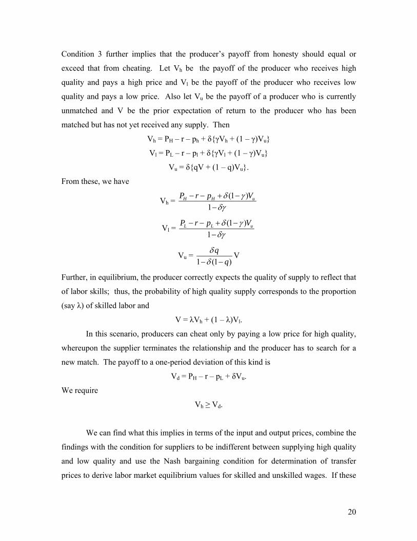
Condition 3 further implies that the producer’s payoff from honesty should equal or
exceed that from cheating. Let Vh be the payoff of the producer who receives high
quality and pays a high price and Vl be the payoff of the producer who receives low
quality and pays a low price. Also let Vu be the payoff of a producer who is currently
unmatched and V be the prior expectation of return to the producer who has been
matched but has not yet received any supply. Then
Vh = PH – r – ph + δ{γVh + (1 – γ)Vu}
Vl = PL – r – pl + δ{γVl + (1 – γ)Vu}
Vu = δ{qV + (1 – q)Vu}.
From these, we have
Vh = (1 )1
H H uP r p Vδ γδγ
− − + −−
Vl = (1 )1
L LP r p Vuδ γδγ
− − + −−
Vu = 1 (1
qq)
δδ− −
V
Further, in equilibrium, the producer correctly expects the quality of supply to reflect that
of labor skills; thus, the probability of high quality supply corresponds to the proportion
(say λ) of skilled labor and
V = λVh + (1 – λ)Vl.
In this scenario, producers can cheat only by paying a low price for high quality,
whereupon the supplier terminates the relationship and the producer has to search for a
new match. The payoff to a one-period deviation of this kind is
Vd = PH – r – pL + δVu.
We require
Vh ≥ Vd.
We can find what this implies in terms of the input and output prices, combine the
findings with the condition for suppliers to be indifferent between supplying high quality
and low quality and use the Nash bargaining condition for determination of transfer
prices to derive labor market equilibrium values for skilled and unskilled wages. If these
20

values are positive, such an equilibrium exists where labor of both skill levels is
employed. We do this calculation in the appendix to show that under certain conditions,
unskilled wages – and therefore skilled wages as well – can indeed be positive.
However, this is by no means a certainty.
Thus in general equilibrium, adjustments in the labor market will change wages
and transfer prices in such a way that we are at the border between a high quality honest
equilibrium and a low quality one : in fact, both high and low quality will in general co-
exist in equilibrium, as long as labor of both kinds exists in the economy, unless of course
the equilibrium wage for unskilled labor is negative – or, as may be easily generalized,
below a minimum subsistence requirement. In the latter case, the model will generate
unemployment. From our calculations in the appendix it is easy to show that
unemployment of unskilled labor becomes likely if the probability of exogenous
separations is very high or if agents are very impatient, as in these circumstances the
unskilled labor wage consistent with employment of both types of labor in general
equilibrium becomes too low to be feasible (in this case, negative).
5. Conclusion
We have applied three models to the analysis of repeated interactions between
homogeneous (optimizing) input suppliers and heterogeneous final goods producers (who
can be either optimizing, or can follow the behavioral rule of always being honest) where
input quality is non-verifiable, producers face uncertain search and deliberate termination
of a match constitutes the main threat against cheating. There is absence of collective
information or memory about cheating. Unlike many other papers, we do not consider
random i.i.d matches every period, but allow relationships to persist in the absence of
exogenous separation or deliberate termination. In our first model, all factors are in
elastic supply and wages and product prices are exogenous : we characterize conditions
supporting (a) a high-quality honest equilibrium, (b) a high-quality equilibrium where
opportunists cheat, (c) a low-quality equilibrium, and (d) a region of multiple equilibria.
We show that returns to cheating are increasing in the proportion of behavioral players in
the population of producers. In our second model, we introduce competition between
21

producers for an inelastic factor, working capital. We show that in many parameter
ranges this generates adverse selection, eliminating some (but not all) behavioral players
– but while limiting the proportion of intrinsically honest players, the strategic response
of input suppliers ensures that universal honesty is enforced. This provides an example
of what happens when strategic and behavioral players belonging to the same class of
agents compete while simultaneously playing a game against another class of agents.
While some “unfit” players may be weeded out, the strategy of these unfit players
becomes universally prevalent owing to the strategic response of the other class of agents.
This response also limits the extent to which “selection” is allowed to operate : not all
behavioral types are eliminated. We also argued that the presence of this channel of
competition could serve as an equilibrium selection device eliminating the multiplicity of
equilibria which obtained for some parameter ranges in the first model. In the second
model, cheating never takes place in equilibrium, and we have either a high quality
honest equilibrium or one with low quality. In our third model, we endogenize wages of
skilled and unskilled labor whose supply we assume to be inelastic so that the wages are
demand-determined. We showed that in general both types of labor are employed in
general equilibrium which constitutes a border between high and low quality equilibria –
both high and low quality are supplied and produced in equilibrium and there is no
cheating. However, if exogenous separation is likely or if agents are impatient, it is
possible to have involuntary unemployment of unskilled labor in general equilibrium so
that high quality alone is produced and only skilled labor is employed.
Appendix A : Calculation of the threshold α*
Given that opportunistic producers have an incentive to cheat (i.e, (16) holds), when
suppliers observe producers on the market, the conditional probability they assign to
such a producer’s honesty is given by (1 )1α γ
αγ−
−. The numerator shows the probability
that the producer is an honest type whose match terminated exogenously (all producers
whose matches were deliberately terminated are of course opportunistic). The
denominator shows the probability of a producer’s being on the market. Now we denote
by V(HQ) the supplier’s payoff to following the strategy of offering high quality:
22

(1 ) (1 ) 1( ) [ ( )] [ ( )]1 1 1 1
H sL s
p wV HQ V HQ p w V HQα γ δ γ α δαγ δγ δ αγ
−− − −= + + − +
− − − −
= 2
(1 )( )1[ ][(1 )(1 ) (1 ) (1 )(1 ) 1
H sL s
p w (1 )( ]p wα γδ ααγ δ αδ γ δ α δ δγ
− −−+ − −
− − − − − − − −
By offering low quality, on the other hand, suppliers get:
V(LQ) = (1 )1 1 1
L u L up w p wδ γδγ δ− −−
+− − −δγ
where the first term simply shows that the supplier gets the low quality payoff if the
match does not break off exogenously, and the second term shows that if the match
breaks off exogenously in any future period, the supplier again gets the low quality
payoff in a new match. This simplifies to
V(LQ) = 1L up w
δ−−
Thus whenever (18) holds, a supplier supplies high quality if and only if V(HQ)
exceeds V(LQ). This happens for a threshold level of α given by
α * = 2( )1 (( ) ( ) {1 1
s u
L uH s L s
w wp wp w p wγ δγ δ
δγ δ δ1 ) }1
γ−
−− −− − − + − +
− − −
(19)
Appendix B : Equilibrium probability of successful search in Model 2
In our second model, some intrinsically honest producers may leave the market in case α
started out being higher than *α and if parameters were such that opportunistic
producers had an incentive to cheat. In this case, let d be the number of honest producers
who “die” or leave the market as a result of competition. Now d solves
*N dN dα α−
=−
where N was the initial number of producers, and α the initial fraction of intrinsically
honest producers. Then in equilibrium, where we necessarily have honesty, the relevant
probability of successful search is now given by
23

(1 )H
MqN d M
γγ
−=
− −
However, if α started out being lower than *α , no “deaths” owing to competition take
place and the probability of successful search remains the same as the Hq of Model 1.
The same is true if parameters are such that a high quality honest equilibrium is sure to
obtain and no one has an incentive to cheat – as there is no destructive competition in this
case either.
Appendix C : Derivation of Wages Consistent with General Equilibrium (Model 3)
with both types of labor being employed
We write Ph for PH – r and Pl for PL – r in order to slightly simplify the notation. For
opportunistic producers not to want to cheat when supplied high quality, we require
(1 )1
h H Uh d
P p VV V Ph L Up Vδ γ δδγ
− + −= ≥ = −
−+
L
Simplifying, this amounts to
( ) (1 )h L U HP p V p pδγ δγ δ− ≥ − + −
Substituting for the transfer prices, using
,2 2
h s lH L
P w P wp p u+ += =
we get
( ) (( ) (1 )2 2 2
l u h l s uh U
P w P P w wP Vδγ δγ δ )− + −− − ≥ − + (A1)
But we also have
H s L up w p w− = −
Or
2 2h s l uP w P w− −
=
h l sP P w w⇒ − = − u . (A2)
Also
24

2 2h s l u
h H lP w P wP p P pL− −
− = = = − (A3)
From (A2),
.( ) (1 )2 2
l uh
P wP Vδγ δγ δ− − ≥ − + −U h lP P (A4)
From (A3),
.h lV V V= =
So
{( ) / 2} (1 )[ ]1 (1 ) 1 (1 ) 1
h h sU
qV P w VqVq q
Uδ δ γδδ δ δγ
− + −= =
− − − − −
or
((1 )(1 ) 2
h sU
P wqVq
)δδ δ δγ
−=
− + − (A5)
From (A4), (A5) and (A2), 2 ( )( )
2 2 2[1 ]l u l u
h hP w q P wP P
qδ γδγ
δ δγ−
− − ≥ + −+ − lP
Solving, 2 2 2 2 2 2[2 2 3 2 ] [2 2 4 2 2 ]
(1 )l h
uq q P q qw δ δγ δ γ δ γ δ δγ δ γ δ γ
δγ δγ+ − − + − + − − +
≤−
P
wu can be positive only if the right hand side of the above inequality is positive. This
requires that
Pl2(1 )qδ δγ
δγ+ − – Ph
2(1 ) 2qδ δγδγ
+ − > 0
Or Pl/Ph > 2(1 ) 22(1 )
δ δγδ δγ
+ −+ −
= 1 – 2(1 )q
δγδ δγ+ −
.
The right hand side of this inequality is decreasing in δ and γ and increasing in q. For a
given configuration of product prices, a positive wu is likelier the lower the exogenous
separation probability and the lower the discount rate and the prospect of finding a new
match in the next period (the latter being in turn an increasing function of the separation
probability). A positive wu in equilibrium implies of course full employment of
unskilled, as well as skilled, labor. Conversely an equilibrium with involuntary
25

unemployment of unskilled labor is more likely if the probability of exogenous separation
is very high or if agents are very impatient.
s u hw w P Pl= + −
or 2 2 2 2 2 2[2 2 4 2 2 ] [2 2 5 2 3 ]
(1 )l h
sq q P q qw δ δγ δ γ δ γ δ δγ δ γ δ γ
δγ δγ+ − − + − + − − +
≤−
P
References
Axelrod, R (1984) : The Evolution of Cooperation. New York. Basic Books.
Diamond, Douglas (1991): “Monitoring and Reputation : the Choice between Bank
Loans and Directly Placed Debt”, Journal of Political Economy,99: 689-721.
Dixit, Avinash (2003) : “On Modes of Economic Governance”, Econometrica, 71(2) :
449-481.
Greif, Avner (1993) : “Contract Enforceability and Economic Institutions in Early Trade :
the Maghribi Traders’ Coalition”, American Economic Review, 83(3) : 525-548.
Grossman, Sanford and Oliver Hart (1986) : “The Costs and Benefits of Ownership : a
Theory of Vertical and Lateral Integration”, Journal of Political Economy, 94 (4): 691-
719.
Guha, Brishti (2005) : “Games Suppliers and Producers Play : Upstream and
Downstream Moral Hazard with Unverifiable Input Quality”, chapter 4 in Malfeasance
and the Market : Essays in Corporate Cheating , PhD thesis, Princeton University.
Gul, Faruk (2001) : “Unobservable Investment and the Hold-up Problem”, Econometrica,
69(2) : 343-376.
Hart, Sergiu (2005) : “Adaptive Heuristics”, Econometrica, 73(5) : 1401-1430.
Maynard-Smith, John (1982) : Evolution and the Theory of Games. Cambridge
University Press, Cambridge.
Myerson, Roger (2004) : “Justice, Institutions and Multiple Equilibria”, Chicago Journal
of International Law, 5 : 91-107.
Samuelson, Larry (1997) : Evolutionary Games and Equilibrium Selection. Cambridge,
Massachusetts. MIT Press.
Williamson, Oliver (1975) : “Markets and Hierarchies : Analysis and Antitrust
Implications”, The Free Press,
26