Strategic Segmentation of Industrial Markets - Gatton College of

Hydrol. Earth Syst. Sci., 17, 665–678, 2013www.hydrol-earth-syst-sci.net/17/665/2013/doi:10.5194/hess-17-665-2013© Author(s) 2013. CC Attribution 3.0 License.

EGU Journal Logos (RGB)

Advances in Geosciences

Open A

ccess

Natural Hazards and Earth System

Sciences

Open A

ccess

Annales Geophysicae

Open A

ccess

Nonlinear Processes in Geophysics

Open A

ccess

Atmospheric Chemistry

and Physics

Open A

ccess

Atmospheric Chemistry

and Physics

Open A

ccess

Discussions

Atmospheric Measurement

Techniques

Open A

ccess

Atmospheric Measurement

Techniques

Open A

ccess

Discussions

Biogeosciences

Open A

ccess

Open A

ccess

BiogeosciencesDiscussions

Climate of the Past

Open A

ccess

Open A

ccess

Climate of the Past

Discussions

Earth System Dynamics

Open A

ccess

Open A

ccess

Earth System Dynamics

Discussions

GeoscientificInstrumentation

Methods andData Systems

Open A

ccess

GeoscientificInstrumentation

Methods andData Systems

Open A

ccess

Discussions

GeoscientificModel Development

Open A

ccess

Open A

ccess

GeoscientificModel Development

Discussions

Hydrology and Earth System

SciencesO

pen Access

Hydrology and Earth System

Sciences

Open A

ccess

Discussions

Ocean Science

Open A

ccess

Open A

ccess

Ocean ScienceDiscussions

Solid Earth

Open A

ccess

Open A

ccess

Solid EarthDiscussions

The Cryosphere

Open A

ccess

Open A

ccess

The CryosphereDiscussions

Natural Hazards and Earth System

Sciences

Open A

ccess

Discussions

Modelling monthly precipitation with circulation weather types fora dense network of stations over Iberia

N. Cortesi1,2, R. M. Trigo 2,3, J. C. Gonzalez-Hidalgo1,4, and A. M. Ramos2,5

1University of Zaragoza, Department of Geography, Zaragoza, Spain2University of Lisbon, CGUL, IDL, Lisbon, Portugal3Universidade Lusofona, Faculdade de Ciencias e Engenharias, Lisboa, Portugal4Instituto Universitario Ciencias Ambientales (IUCA), University of Zaragoza, Zaragoza, Spain5University of Vigo, Ephyslab, Vigo, Spain

Correspondence to:J. C. Gonzalez-Hidalgo ([email protected])

Received: 30 March 2012 – Published in Hydrol. Earth Syst. Sci. Discuss.: 4 June 2012Revised: 8 January 2013 – Accepted: 23 January 2013 – Published: 13 February 2013

Abstract. Precipitation over the Iberian Peninsula (IP) ishighly variable and shows large spatial contrasts between wetmountainous regions to the north, and dry regions in the in-land plains and southern areas. In this work, we modelled therelationship between atmospheric circulation weather types(WTs) and monthly precipitation for the wet half of the year(October to May) using a 10 km grid derived from a high-density dataset for the IP (3030 precipitation series, overallmean density one station each 200 km2). We detected twospatial gradients in the relationship between WTs and pre-cipitation. The percentage of monthly precipitation explainedby WTs varies from northwest (higher variance explained) tosoutheast (lower variance explained). Additionally, in the IPthe number of WTs that contribute significantly to monthlyprecipitation increase systematically from east to west. Gen-erally speaking, the model performance is better to the westthan to the east where the WTs approach produce the lessaccurate results. We applied the WTs modelling approach toreconstruct the long-term precipitation time series for threemajor stations of Iberia (Lisbon, Madrid, Valencia).

1 Introduction

Understanding precipitation variability is crucial for a num-ber of reasons, namely: to assess recent significant climatetrends and predictions, to calibrate regional models, to quan-tify changes in the hydrological cycle and to develop na-tional and regional water planning. However, precipitation

variability is difficult to assess because precipitation is oneof the climate elements with highest variability at temporaland spatial scale. This explains the generalised recommen-dation of using high density precipitation database for re-gional analyses (Auer et al., 2005; Brunetti et al., 2006). InEurope one of the most interesting areas to study precipita-tion variability is the Iberian Peninsula (IP) because of itslatitudinal location (between tropical and mid-latitudes), itswestern position contrasting between two water bodies (At-lantic ocean and Mediterranean Sea), and also because thedisposition of the main relief chain in central and western ar-eas is West-East, while to the East the relief is North-South.Thus, precipitation in the IP exhibits high variability at spa-tial and temporal domains (de Castro et al., 2005; de Luis etal., 2008).

In the IP precipitation presents the largest concentra-tion from October to May, mainly due to the baroclinicsynoptic-scale perturbations moving eastward from the At-lantic Ocean, although meso-scale convective systems canalso be responsible for high rainfall rates in the eastern halfof the Iberian Peninsula (Paredes et al., 2006; Garcıa-Herreraet al., 2005). In contrast, the scarce summer precipitation ismostly due to local factors and convective storms (Serranoet al., 1999). Furthermore, seasonal precipitation regimesin the IP exhibit a great variability, and dramatic changesduring the second half of the 20th century have been de-tected, mostly as a consequence of the significant decrease ofspring precipitation (de Luis et al., 2010). For these reasons,rainfall spatial variability in the IP is best detected using a

Published by Copernicus Publications on behalf of the European Geosciences Union.

666 N. Cortesi et al.: Modelling monthly precipitation with circulation weather types

spatially dense network of observations (Valero et al., 2009;Gonzalez-Hidalgo et al., 2009).

In recent years, significant efforts were made to reproduceprecipitation behaviour in Europe with a particular focus inthe IP from daily to seasonal scales (Spellman, 2000; Trigoand DaCamera, 2000; Goodess and Jones, 2002; Santos etal., 2005; Paredes et al., 2006; Lorenzo et al., 2008), us-ing an array of methods including circulation weather types(WTs). The usefulness of WTs classification has been in-vestigated for a wide range of applications in scientific do-mains, from climate to environmental areas such as air qual-ity and natural hazards, such as forest fires, floods, droughts,avalanches and storm lightning (e.g., Vicente-Serrano andLopez-Moreno, 2006; Demuzere et al., 2009; Prudhommeand Genevier, 2011; Kassomenos, 2010; Ramos et al., 2011).From an hydrological perspective, WTs classifications havebeen used for different purposes, including their relation withprecipitation (e.g., Hanggi et al., 2011; Andrade et al., 2011),extreme precipitation events (Mauran et al., 2010), forestgrowth (Pasho et al., 2011), drought (e.g., Fowler and Kilsby,2002; Fleig et al., 2011) and river discharge, including floods(e.g., Wilby, 1993; Auffray et al., 2011; Fowler et al., 2000).

The main objective of all circulation classificationschemes is to provide fast, objective and reproducible meth-ods for categorising the continuum of atmospheric circula-tion into a reasonable and manageable number of discreteclasses (types). Different methods exist for the classifica-tion of WTs, as was shown by Yarnal et al. (2001), Huth etal. (2008), and Phillip et al. (2010). These different method-ological approaches can be categorised by the kind of typedefinition they use that can range from pure statistical (e.g.,Cluster analysis and PCA) or dynamic based (e.g., intensityand direction of geostrophic wind and vorticity).

Regarding the use of WTs classification for downscaling,Bardossy and Pegram (2011) define procedures to give con-fidence in the interpretation of such rainfall estimates mod-elled by global circulation models (GCMs). They use cir-culation patterns to define quantile-quantile transforms be-tween observed and GCMs estimated rainfall in present cli-mate and to estimate the rainfall patterns in future scenar-ios. Wilby (1998) modelled low-frequency rainfall eventsby means of airflow indices, WTs classifications and frontalfrequencies. Distinct circulation weather type clusters wereidentified and used to construct a simplified model of dailyprecipitation amount. The model was calibrated against grid-ded data for the period 1970–1990 and used to reconstructdaily precipitation between 1875 and 1969 given the historicsequence of WTs.

In the Iberian Peninsula, Goodess and Palutikof (1998) de-veloped a Markov Chain model to reconstruct daily precipi-tation at 20 locations in Guadalentın Basin (SE Spain) using8 WTs as predictor variables. Trigo and DaCamara (2000)introduced a multiple regression model based on the threewettest WTs frequencies (the cyclonic, the south westerlyand the westerly types) as predictor variables to reconstruct

monthly winter rainfall totals for 18 key sites in Portugal.Spellman (2000) performed a stepwise regression analysison a catalogue of air flow indexes to estimate monthly meanrainfall amounts for IP. Goodess and Jones (2002) expandedthe regression model to include up to 14 circulation weather-types frequencies with a forward selection method based onthe F-test and applied to 20 Iberian stations. Finally, Santos etal. (2005) developed a K-mean cluster analysis over the firstthree principal components of the daily sea-level pressureweighted anomalies to isolate 5 weather regimes responsi-ble for the inter annual variability of monthly winter rainfallamounts.

However, all the above-mentioned works addressing thelink between monthly winter precipitation and atmosphericcirculation patterns relied on very low density observationnetworks to validate their models, typically less than 50 sta-tions for the whole IP. In this regard, it is perfectly reason-able to state that the spatial detail required for hydrolog-ical planning, soil erosion and many other purposes werenot well captured. Also spring, summer and autumn precip-itation variability have been less explored; notwithstandingOctober–May is the rainiest period in many areas in the IP(de Luis et al., 2010). In this sense, the recent developing ofa high density spatial database of monthly precipitation inthe IP combining Portugal and Spanish land (see Gonzalez-Hidalgo et al., 2011 and Lorenzo-Lacruz et al., 2011) pro-vides, for the first time, an opportunity to fill this gap andfacilitates the relationships between weather types and pre-cipitation totals at high spatial detail.

The research is conducted not on precipitation variabil-ity itself, but on the nature of its variability. Accordingly,the objective of this paper is twofold: firstly modelling therelationship between the monthly frequency of WTs andmonthly precipitation with the highest spatial detail availableat present in the IP; and secondly to show the usefulness ofsuch an approach in long-term precipitation reconstruction.This paper is the starting step in providing the opportunity ofextending the reconstruction of monthly precipitation for avery high density of stations as far back in time as 1850, be-cause catalogues of circulation weather types are now avail-able since then. These reconstructions at high spatial detailwould provide, in the near future, the long-term contextualframework of precipitation variability and trends in the IP,thus, allowing considering the recent changes of precipita-tion monthly distribution within a more global context fromthe middle of the 19th century. Therefore, while the maineffort of this paper is focused on the evaluation of modelsperformance during the 1948–2003 period, we will also as-sess the potential of this modelling approach by applying thevalidation with three of the longest series of monthly precip-itation available in the IP.

The paper is organised as follows: section 2 describes thedata, the circulation weather types used, the description ofthe model and the validation method. Section 3 analysesthe model performance and the relative contribution to total

Hydrol. Earth Syst. Sci., 17, 665–678, 2013 www.hydrol-earth-syst-sci.net/17/665/2013/

N. Cortesi et al.: Modelling monthly precipitation with circulation weather types 667

monthly precipitation by each WT. In Sect. 4, we apply themodel to reconstruct long-term precipitation for 3 stations(Lisbon, Madrid, Valencia). Finally, Sect. 5 contains a sum-mary of the main results and the concluding remarks.

2 Database, Weather Types and methods

2.1 Precipitation data

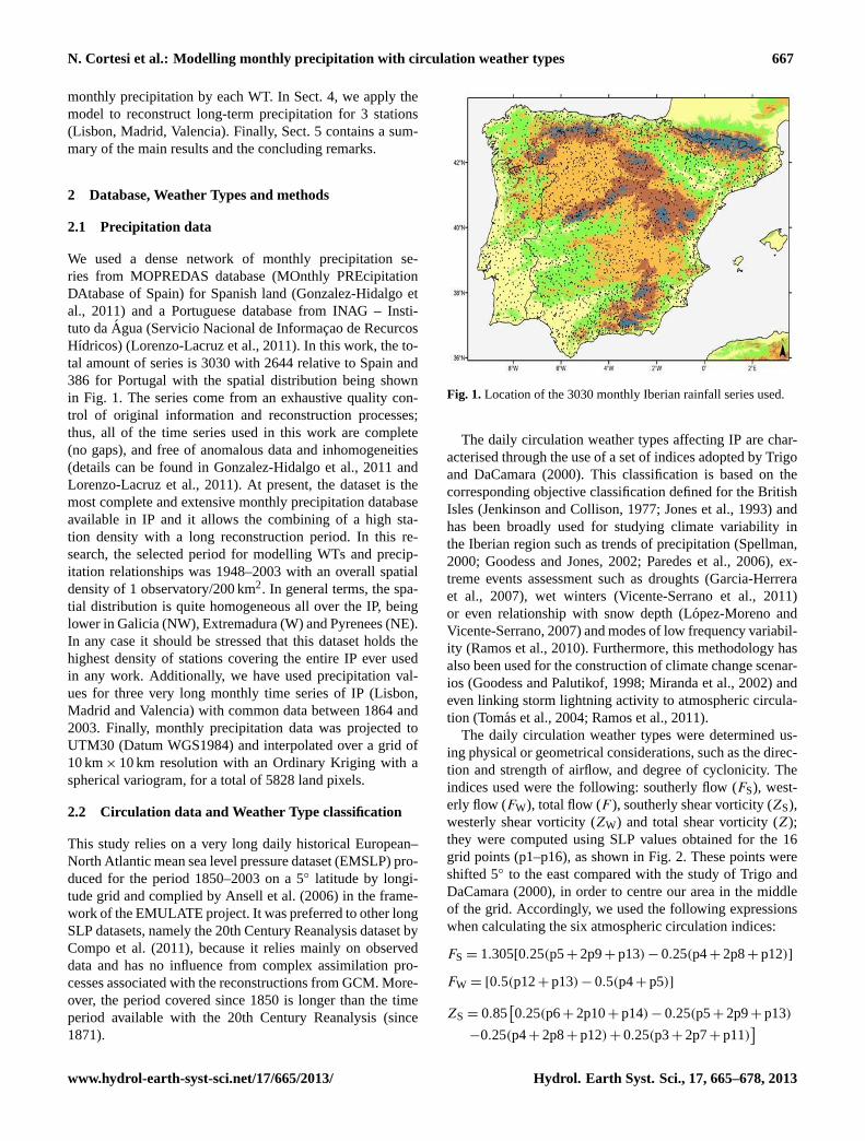
We used a dense network of monthly precipitation se-ries from MOPREDAS database (MOnthly PREcipitationDAtabase of Spain) for Spanish land (Gonzalez-Hidalgo etal., 2011) and a Portuguese database from INAG – Insti-tuto daAgua (Servicio Nacional de Informacao de RecurcosHıdricos) (Lorenzo-Lacruz et al., 2011). In this work, the to-tal amount of series is 3030 with 2644 relative to Spain and386 for Portugal with the spatial distribution being shownin Fig. 1. The series come from an exhaustive quality con-trol of original information and reconstruction processes;thus, all of the time series used in this work are complete(no gaps), and free of anomalous data and inhomogeneities(details can be found in Gonzalez-Hidalgo et al., 2011 andLorenzo-Lacruz et al., 2011). At present, the dataset is themost complete and extensive monthly precipitation databaseavailable in IP and it allows the combining of a high sta-tion density with a long reconstruction period. In this re-search, the selected period for modelling WTs and precip-itation relationships was 1948–2003 with an overall spatialdensity of 1 observatory/200 km2. In general terms, the spa-tial distribution is quite homogeneous all over the IP, beinglower in Galicia (NW), Extremadura (W) and Pyrenees (NE).In any case it should be stressed that this dataset holds thehighest density of stations covering the entire IP ever usedin any work. Additionally, we have used precipitation val-ues for three very long monthly time series of IP (Lisbon,Madrid and Valencia) with common data between 1864 and2003. Finally, monthly precipitation data was projected toUTM30 (Datum WGS1984) and interpolated over a grid of10 km× 10 km resolution with an Ordinary Kriging with aspherical variogram, for a total of 5828 land pixels.

2.2 Circulation data and Weather Type classification

This study relies on a very long daily historical European–North Atlantic mean sea level pressure dataset (EMSLP) pro-duced for the period 1850–2003 on a 5◦ latitude by longi-tude grid and complied by Ansell et al. (2006) in the frame-work of the EMULATE project. It was preferred to other longSLP datasets, namely the 20th Century Reanalysis dataset byCompo et al. (2011), because it relies mainly on observeddata and has no influence from complex assimilation pro-cesses associated with the reconstructions from GCM. More-over, the period covered since 1850 is longer than the timeperiod available with the 20th Century Reanalysis (since1871).

Figure_1. Location of the 3030 monthly Iberian rainfall series.

Fig. 1.Location of the 3030 monthly Iberian rainfall series used.

The daily circulation weather types affecting IP are char-acterised through the use of a set of indices adopted by Trigoand DaCamara (2000). This classification is based on thecorresponding objective classification defined for the BritishIsles (Jenkinson and Collison, 1977; Jones et al., 1993) andhas been broadly used for studying climate variability inthe Iberian region such as trends of precipitation (Spellman,2000; Goodess and Jones, 2002; Paredes et al., 2006), ex-treme events assessment such as droughts (Garcia-Herreraet al., 2007), wet winters (Vicente-Serrano et al., 2011)or even relationship with snow depth (Lopez-Moreno andVicente-Serrano, 2007) and modes of low frequency variabil-ity (Ramos et al., 2010). Furthermore, this methodology hasalso been used for the construction of climate change scenar-ios (Goodess and Palutikof, 1998; Miranda et al., 2002) andeven linking storm lightning activity to atmospheric circula-tion (Tomas et al., 2004; Ramos et al., 2011).

The daily circulation weather types were determined us-ing physical or geometrical considerations, such as the direc-tion and strength of airflow, and degree of cyclonicity. Theindices used were the following: southerly flow (FS), west-erly flow (FW), total flow (F ), southerly shear vorticity (ZS),westerly shear vorticity (ZW) and total shear vorticity (Z);they were computed using SLP values obtained for the 16grid points (p1–p16), as shown in Fig. 2. These points wereshifted 5◦ to the east compared with the study of Trigo andDaCamara (2000), in order to centre our area in the middleof the grid. Accordingly, we used the following expressionswhen calculating the six atmospheric circulation indices:

FS = 1.305[0.25(p5+ 2p9+ p13) − 0.25(p4+ 2p8+ p12)]

FW = [0.5(p12+ p13) − 0.5(p4+ p5)]

ZS = 0.85[0.25(p6+ 2p10+ p14) − 0.25(p5+ 2p9+ p13)

−0.25(p4+ 2p8+ p12) + 0.25(p3+ 2p7+ p11)]

www.hydrol-earth-syst-sci.net/17/665/2013/ Hydrol. Earth Syst. Sci., 17, 665–678, 2013


Figure_2. Location of the 16 grid points used to compute the vorticity and flow indices. Fig. 2.Location of 16 grid points used to compute the vorticity andflow indices.

ZW = 1.12[0.5(p15+ p16) − 0.5(p8+ p9)]

−0.91[0.5(p8+ p9) − 0.5(p1+ p2)]

F = (FS2+ FW2)1/2

Z = ZS+ ZW

The conditions established to define different types of cir-culation are the same as those imposed in Trigo and DaCa-mara (2000), and the following set rules were used:

1. Direction of flow was given by tan−1 (FW/FS), 180◦ be-ing added ifFW was positive. The appropriate directionwas computed using an eight-point compass, allowing45◦ per sector.

2. If | Z | < F , the flow is essentially straight and was con-sidered to be of a pure directional type (eight differentcases, according to the directions of the compass).

3. If | Z | > 2F , the pattern was considered to be of a purecyclonic type ifZ > 0, or of a pure anticyclonic type ifZ < 0.

4. If F < | Z | < 2F , the flow was considered to be of ahybrid type and was, therefore, characterised by bothdirection and circulation (8× 2 different types).

The indices and rules mentioned allow us to define 26 dif-ferent circulation Weather Types (WTs) at daily scale and forthe study period, grouped in three main classes: eight puredirectional types defined by their direction: N, NE, E, SE, S,SW, W and NW, two pure types controlled by the strengthof geostrophic vorticity (cyclonic C and anticyclonic A), andsixteen hybrid types (eight cyclonic and eight anticyclonicfor each direction (see Fig. 3). Unlike some other authors(Jenkinson and Collison, 1977; Jones et al., 1993), an un-classified class was not defined, opting to disseminate thefairly few cases (< 2 %) with possibly unclassified situationsamong the retained classes. This was done in order to solve

the problem of the sudden increase in the unclassified classduring summer for IP with Jenkinson and Collison’s methoddetected by Martin-Vide (2002) and caused by the domi-nant low-pressure summer gradient over IP (Hoinka and Cas-tro, 2003). Another weakness of Jenkinson and Collison’smethod is related to the absence of pressure data at otherlevel than SLP, which can cause to obtain a high frequencyof cyclonic days (both pure and hybrid) during the summermonths in some IP areas, as a consequence of frequent lowpressures at surface level during this season (Capel, 2000).Nevertheless, we found that this problem does not affect theIP when studied as a whole: summer frequencies for the com-bined 9 cyclonic WTs are always below 3 days per month.

For model performance it is often recommended to useclassifications with a smaller number of WTs, because in thiscase each predictor WT benefits of a higher number of daysper month potentially improving the reliability of their usein regression analyses. However, that was not the case in thiswork, thus, when we tried this approach with 8 directionalWTs and pure A and pure C (10 WTs) the resulting modelperformance, measured with the normalised MAE score (seeSect. 2.3), was 9.3; for 8 directional WTs, 8 cyclonic WTsand pure A and pure B (i.e., 18 WTs) it was found to be8.9; and finally the MAE with 26 WTs was 8.5. This meansthat 26 WTs improved the regression performance up to 8 %compared to what was achieved using 10 WTs only, so theclassification with 26 WTs was selected for all the followinganalysis.

2.3 The model

The analysis was applied individually to all 5828 Iberiangridded precipitation time series and for the autumn, winterand spring months (strictly speaking from October to May),because most IP precipitation falls within these months(roughly 80 %), and because absolute amounts of precipita-tion due to convective processes are relatively lower duringthe selected months. Moreover, the IP changes in summerrainfall cannot always be explained by changes in circula-tion, given that local factors play a major role (Mosmann etal., 2004). Interpolation of monthly precipitation was nec-essary because the spatial distribution of observations is notperfectly homogeneous over the IP. Finally, monthly analysiswas preferred, because seasonal behaviour often masks dif-ferent monthly behaviour in the IP precipitation (Serrano etal., 1999; Goodess and Jones, 2002; Gonzalez-Hidalgo et al.,2009; de Luis et al., 2010).

The model selected was a multiple linear regression(with a stepwise forward selection procedure) adapted fromthat of Trigo and DaCamara (2000) and of Goodess andJones (2002). It considers the monthly frequencies (as num-ber of days/month) of each of the 26 WTs as predictor vari-ables, and the corresponding vector of monthly rainfall totalsas the predicted variable along the study period 1948–2003(Eq. 1).



Year Observed WT1 WT2 WT26∣∣∣∣∣∣∣∣1948:

1949:

...

2003:

14901167...

1388

= α0 + α1 ·

914...

8

+ α2 ·

1712...

20

+ ... + α26

15...

3

(1)

with α0 ≥ 0 the constant term andα1...α26 ≥ 0 the coeffi-cients for the different WTs that represent their mean dailyrainfall amount (mm day−1).

The regression coefficients solve the non-negative least-squares problem min‖ Aα − α0 ‖, with α = (α1,...,α26) andA matrix of 26 column and 56 rows with the monthly WTfrequencies. Coefficients were constrained as non-negativebecause they physically represent the mean daily rainfallamount due to the correspondent WT (that is non-negativeby definition). The constant termα0 was also constrainedas non-negative, to reflect the rain amount due to other pro-cesses that can not be modelled by individual WTs. Up to amaximum of ten predictors were selected for individual pix-els.

We selected the stepwise forward selection procedure be-cause the model performance largely depends on the in-put variables (von Storch and Zwiers, 1999), and it ensuresthat only relevant predictors are incorporated into the regres-sion model. We followed this approach following Efroym-son (1960) because in our case there are a large number ofpotential explanatory variables and no underlying theory onwhich to base the predictor’s selection. The stepwise for-ward procedure also minimises the risk of over fitting ofWTs in the regression, separates noise from the dominanttemporal patterns of variability, and removes highly corre-lated predictor variables from the subset of predictors chosenfor a given grid point and month. Accordingly, the selectionof WTs was as follows: at each stepk in the process, wechecked if each new potential predictor (WTs) contributiondecreased the Root Mean Square Error or RMSE (see Wilks,2006, Chapter 6.4.3.) for the selected pixelp, monthm andregression stepk, as follows:

RMSE(p,m,k) =

√√√√√ n∑i=1

(Pi(p,m,k) − Oi(p,m))2

N(2)

with P andO being two vectors with the respectively pre-dicted and observed monthly precipitation values for all theN = 56 yr of the regression period (1948–2003). Remem-ber that the RMSE is a non-negative number that tends to0 when there is perfect agreement between reconstructionsand observations. If the regression residualsPi − Oi followa Gaussian distribution, the RMSE is also equal to the er-ror’s standard deviation of the reconstruction. The Shapiro-Wilk normality test applied to all grid points and monthsfound that the residuals are normally distributed only if theRMSE of the chosen pixel and month is low (about 40 % of5828· 8 months = 46 624 residual time series passed the test).

Figure_3. Composite map of the daily SLP average fields for the eight directional

weather types (NW, N, NE, E, SE, S, SW, W) and two vorticity weather types (C and

A). Hybrid types are not shown. Contour interval is 2 hPa.

Fig. 3. Composite map of the SLP fields for the eight directionalweather types (NW, N, NE, E, SE, S, SW, W), and two vorticityweather types (C and A). Hybrid types are not shown.

At the end of the selection of the best predictor WTs, asmall number of them (10 %) were still moderately corre-lated (r ≈ 0.4–0.6). Usually, to overcome multicollinearityproblems, “...whichever of the two high correlated WTs ispicked at a later regression step is omitted from the final setof predictor variables” (Goodess and Jones, 2002). However,to minimise multicollinearity without removing a priori anyWTs, we stopped the stepwise regression when the new vari-able introduced at a given stepk did not decrease the RMSEof at least one hundredth the mean monthly observed precip-itation in comparison to the RMSE of the previous stepk−1.This threshold is equivalent to improve the RMSE of 10 mmof precipitation when the mean monthly observed precipita-tion is 1000 mm (i.e., 1 %). In this way, any correlated WTsmay be excluded from the regression for some grid pointsif they do not improve the RMSE, but may be included inthe regression model relative to other pixels if they improvethe RMSE, even if we know that they are highly correlated.In brief, the proposed threshold value was chosen because atthe same time it minimised the numbers of predictors (reduc-ing over fitting and multicollinearity) without significantly



decreasing the model performance measured by the RMSEscore.

Even with minimised over fitting, multicollinearity canstill affect 1–2 predictor WTs, depending from month andgrid time series. Heteroscedasticity is also present and in-creases error variances for large precipitation values. Fur-thermore, for WTs that are not chosen as predictors, theirpredicted monthly rainfall amount is exactly zero mm, whilein reality they often contribute to a few mm of precipitation.On the contrary, selected predictor WTs have to also accountfor the rainfall contribution of the excluded WTs, resultingin an overestimation of their predicted precipitation. Finally,another poor feature of the predicted time series is the rel-atively under-prediction of interannual variability in easternIP, where for each month the predicted standard deviationsare significantly lower (up to ten time smaller) than observedfor the majority of time series (not shown, but with a spatialpattern similar to Fig. 4).

Model validation was performed by means of a leave-one-out cross validation over the regression period for all 5828grid time series of monthly precipitation of IP. Specifically,for each pixel and month the experiment was carried out wasas follows: one year of monthly precipitation data was ex-cluded, and then we estimated the model parameters for theremaining years and the predicted precipitation for the yeardiscarded was then calculated.

The use of the RMSE also as indicator of goodness ofmodel should be avoided, because it varies with variabilityin the squared errors, so it is impossible to discern the degreeto which the RMSE reflects average errors and to what ex-tent it reflects variability in the distribution of squared errors(Willmott and Matsuura, 2005 and 2006). Instead, we eval-uated the model performance with three error indexes: theMean Absolute Error (MAE), the Mean Bias Error (MBE)and theD of Willmott (also called “Index of Agreement”).MAE index is less sensitive to large reconstruction errorsthan the RMSE and describes the average error alone. It canrange from 0 to infinity and, of course, lower values are bet-ter. MBE provides relevant information about the averageover- or under-prediction, so it can assume also negative val-ues. Willmott’sD scales with magnitude of the variables, isbounded between 0 and 1 (perfect prediction), retains meaninformation and does not amplify outliers (Willmott, 1981,1982; Willmott et al., 2012). Computational forms of thethree indexes are given below:

MAE(pm) = O(p,m)−1

N−1N∑

i=1

|Pi(p,m) − Oi(p,m)| (3)

MBE(pm) = O(p,m)−1

N−1N∑

i=1

(Pi (p,m) − Oi (p,m)) (4)

D(p,m) =

N∑i=1

|Pi(p,m) − Oi(p,m)|

N∑i=1

(|Pi(p,m) − O(p,m)|+|Oi(p,m) − O(p,m)|)

(5)

WhereO is the mean monthly observed precipitation dur-ing the study period. Both MBE and MAE were normalisedfor O to compare values obtained for different pixels andmonths, while the form ofD in Eq. (5) is the modified Indexof Agreement suggested by Willmott et al. (1985), which ismuch less sensitive to outliers than the original formulation.

3 Results

3.1 Model validation

The results of the cross-validation analysis are shown in thefollowing set of Figs. 4 and 5 that focus on different aspectsof the evaluation procedure. The area with the lowest MAE-values (< 5 % ofO) is located to the northwest (north of Por-tugal and Spanish border, Fig. 4). Also low MAE-values be-tween 5 % and 10 % can be observed to the north, west andsouthwest except in April and May, when high values are re-stricted to the northern areas of Portugal, and surroundingareas of Spain. The highest values are found in the Mediter-ranean fringe although the area with MAE> 15 % varies be-tween months. It is interesting to notice that the Ebro basinto the northeast inland of IP usually exhibits moderate MAE-values ranging between 10 %–15 %. In general the spatialrange of MAE-values increases in April and May suggest-ing that spring precipitation depends more on local factorsthan on synoptic patterns of atmospheric circulation.

The obtained spatial pattern of MAE parameter suggeststhat the capacity of using regional atmospheric circulationto explain the Iberian precipitation regime decreases signifi-cantly along an axis predominately from northwest to south-east.

For each month, the distribution of the MBE is quite het-erogeneous and does not show any clear spatial pattern in theIP (figure not shown); normalised MBE is greater than±2 %only for 4.6 % of pixel-month pairs and greater than±5 %only for 0.4 % of cases.

The spatial distribution of Willmott’sD presents rela-tively similar results to those attained by MAE. In particu-lar theD scores obtained for the 5828 time series also re-veal a main gradient oriented NW–SE (Fig. 5). The highestD-values, corresponding to better model performance, are lo-cated along the Atlantic and northern Cantabric coast to thenorthwest (a maximum of 0.86 in December at Quinta For-mosa, north of Portugal), while the lowest D-values are foundon the Mediterranean coast (a minimum of 0.09 in Octoberat Tuejar, west of Valencia, Spain). During April and May,the areas with the lowest D-values spread along the southern



Figure 4. Spatial and temporal distribution of MAE of predicted rainfall amount for

each month from October to May normalized for the mean monthly observed

precipitation. Low percentages represent a better agreement between reconstruction and

observations.

Fig. 4. Spatial and temporal distribution of MAE of predicted rain-fall amount for each month from October to May normalised for themean monthly observed precipitation. Low percentages represent abetter agreement between reconstruction and observations.

coastland areas (Andalucıa) and the Ebro Valley up to theCantabric Coast.

A monthly comparison of the goodness of the predictionsfor the whole IP can be found in Table 1. Each of the threemonthly error indexes was averaged over all the 5828 IP pix-els. Although spatial information is lost, this table allowsidentifying which month is better reconstructed: Decem-ber (normalised MAE = 7.7 %, MBE = 0.0 % andD = 0.65),while February and May are the months with the poorest per-formance, having the highest MAE and lowerD index, re-spectively.

3.2 Number and type of predictor WTs

The spatial distribution of the number of predictors retained(i.e., WT) for the models are shown for each month in Fig. 6.A small number of time series (5 %) were modelled with onepredictor only; all of them are concentrated over the Mediter-ranean Coast. Time series with 2 predictors are spread over awider area (17 %), particularly in March. However, the most

Figure 5. Spatial and temporal distribution of D of Willmott applied to predicted and

observed precipitation for each month from October to May. High values near 1

represent a better agreement between reconstruction and observations. Fig. 5.Spatial and temporal distribution WillmottD applied to pre-dicted and observed precipitation for each month from October toMay. High values near 1 represent a better agreement between re-construction and observations.

Table 1. Global monthly normalised MAE, MBE and D indexesfrom October to May. Each index was averaged over all the 5828pixels.

Index Oct Nov Dec Jan Feb Mar Apr May

MAE 8.2 % 8.0 % 7.7 % 8.5 % 9.3 % 9.0 % 8.6 % 9.1 %MBE 0.1 % −0.2 % 0.0 % 0.1 % −0.2 % 0.4 % 0.0 % 0.2 %D 0.60 0.60 0.65 0.63 0.61 0.62 0.52 0.48

frequent time series are those characterised with 3 predictors(28 %), being homogeneously distributed all over IP. On theother side models requiring either 4 predictors (24 % of pix-els) or 5 predictors (15 %) tend to be clustered in the westernand central sectors of IP. Models with 6 predictors (6 %) areusually not found on the Mediterranean Coast, but are nu-merous in Portugal and Andalusia in southern Spain. Finally,models requiring up to 7 and 8 predictors (the 1 % and 0.2 %,respectively) are mostly confined to southern Portugal.

In general terms, there is a rough longitudinal spatial gra-dient in the number of WTs from West (more) to the East(less) (Fig. 7). Temporally, the mean number of WTs scores



Figure 6. Spatial and temporal distribution of the number of predictor WTs of the

regression model for each month from October to May. Fig. 6. Spatial and temporal distribution of the number of predictorWTs of the regression model for each month from October to May.

its maximum in October (3.9 WTs mean value), Novem-ber (3.8 WTs), December (3.6 WTs) and January (3.5 WTs),while the minimum value correspond to May (2 WTs),March (2.8 WTs) and April (2.9 WTs). Usually time serieswith a high number of WTs have lower MAE scores thanseries with few predictors.

For a given time series and month, the mean predictedrainfall amount of thei-esim WT can be obtained by mul-tiplying its regression coefficientαi in Eq. (1) for its meanmonthly frequency (as number of days in a month) duringthe study period 1948–2003. This value can be normalisedfor the mean observed precipitation to get the mean percent-age of WT predicted rainfall for the given pixel and month.Averaging these values for all the 5828 time series duringthe same month we obtain the mean monthly percentage ofmodelled precipitation by WT over all Iberian Peninsula, pre-sented in Table 2. Please note that columns do not sum to 100because we did not include the constant term and, addition-ally, because values are calculated dividing the amount (mm)

Table 2. Average estimated WT percentage contribution to totalmonthly Iberian precipitation during 1948–2003.

WT Oct Nov Dec Jan Feb Mar Apr May Mean

NE 1.1 0.9 0.2 0.0 0.4 1.2 0.8 0.2 0.6E 0.1 0.1 0.0 0.8 4.0 0.6 0.2 0.0 0.7SE 0.1 0.7 0.2 0.4 0.2 0.1 0.1 0.0 0.2S 3.7 0.6 0.3 0.5 0.7 0.1 0.0 2.4 1.0SW 8.1 7.3 15.9 18.9 14.6 8.8 6.0 3.3 10.4W 19.0 19.0 23.8 27.9 28.7 31.1 13.2 13.4 22.0NW 1.0 10.4 6.1 8.5 1.4 0.4 3.3 4.5 4.4N 3.2 1.2 0.9 2.6 1.6 6.9 0.9 8.1 3.2

Sum 36.3 40.2 47.4 59.6 51.6 49.2 24.5 31.9 42.5

C 11.5 12.7 9.9 18.1 2.6 13.4 23.2 20.9 14.0C.NE 1.6 0.1 1.5 0.0 0.0 1.4 3.5 2.3 1.3C.E 4.2 1.8 2.5 0.2 1.2 0.5 0.4 0.2 1.4C.SE 0.7 2.4 4.2 0.2 1.2 0.5 0.4 0.2 1.2C.S 0.7 3.4 0.2 0.1 0.1 1.0 0.0 0.3 0.7C.SW 2.7 6.3 3.2 1.1 4.1 1.6 0.4 0.1 2.4C.W 6.5 2.2 0.6 1.0 0.5 0.3 0.0 0.7 1.5C.NW 1.2 0.0 1.1 0.1 1.2 0.0 0.8 0.8 0.7C.N 0.3 0.5 0.4 0.0 3.0 0.0 0.0 0.2 0.6

Sum 29.4 29.4 23.6 20.7 13.4 18.4 29.3 25.9 23.8

A 0.1 0.0 0.0 0.0 0.0 0.1 0.0 0.0 0.0A.NE 0.8 0.0 0.0 0.1 0.0 0.0 0.6 1.5 0.4A.E 0.0 0.2 0.0 0.0 0.4 0.0 0.0 0.5 0.1A.SE 0.0 0.2 0.0 0.0 0.0 0.0 0.4 0.1 0.1A.S 0.0 0.0 0.0 0.0 0.2 0.5 0.5 0.0 0.2A.SW 0.0 0.0 0.1 0.6 0.2 0.1 0.0 0.0 0.1A.W 0.4 0.8 0.4 0.1 0.2 2.4 1.8 0.0 0.8A.NW 1.4 1.4 1.3 0.8 0.1 0.1 0.4 0.1 0.7A.N 0.1 0.7 0.4 0.1 0.2 0.0 0.7 0.0 0.3

Sum 2.7 3.1 2.3 1.7 1.3 3.1 4.4 2.2 2.7

Total 68.4 72.7 73.3 82.0 66.3 70.7 58.2 60.0 69.1

of precipitation predicted by the amount (mm) of precipi-tation observed. The percentage of relative contribution ofeach WT to the observed monthly precipitation varies con-siderably from pixel to pixel and from month to month. Theglobal monthly relative contribution of all WTs can be foundin the last row of Table 2. The highest global values are foundin January (82.0 %), the lowest in April (58.2 %). On av-erage, the global relative contribute of all 26 WTs to meanmonthly rainfall from October to May is about 69.1 %, andthe four wettest WTs contribute around 50 % to total monthlyprecipitation, namely the westerly (22.0 %), Pure Cyclonic(14.0 %), southwesterly (10.4 %) and northwesterly (4.4 %)(see column Mean of Table 2).

The contribution of westerly (W) weather types rise grad-ually from October to March and then decrease until April–May when the lowest values are reached; the same pattern isobserved with the southwesterly (SW), while the maximumis achieved in January. On the contrary, the contribution ofNW and N types shows high monthly oscillations from Octo-ber to May (maximum in November and May, respectively).Pure cyclonic (C) type is a special case because it dropsabruptly to 2.6 % in February, while during all other monthsit never falls below 9 % and maximum value are achieved inApril–May.



It is worth noting that on a monthly average, the 8 direc-tional WTs contribute to 42.5 % of total monthly precipita-tion, the 9 cyclonic WTs contribute to 23.8 %, while the 9 an-ticyclonic WTs only contribute 2.7 %. On the other hand, themaximum mean value relative contribution to total precipi-tation of directional WTs can be observed in winter months,while for cyclonic WTs this maximum contribution is locatedin spring or autumn months.

With the aim of summarising results, we present inFig. 7, the spatial distribution of relative WTs contributionto monthly precipitation. The mean value of the precipitationcontribution by the WTs identified by model, irrespectivelyof their number, suggests some interesting features at spatiallevel. In central, western and southwestern areas the meanvalue contribution of WTs to monthly precipitation is usu-ally over 70 %, and sometimes even above 90 %. However, ina few restricted areas less than 50 % of monthly precipitationis reproduced by the WTs based models, particularly alongthe Mediterranean coast, and inland areas such as the EbroBasin, particularly in February, April and May. A second in-teresting result can be appreciated in the northern mountain-ous sector of Iberia; this area is very humid, but the WTs onlyreproduce a maximum of 70 % of monthly precipitation thatcould be due to a systematic effect of mountain chain parallelto the coast enhancing a local forcing.

The spatial variation of the different WTs contribution tomonthly precipitation is high. We present an example for Jan-uary (Fig. 8) because this is the month in which the modelprediction achieves higher proportion of total precipitationby WTs (82.0 %).

During January the selected WTs vary greatly from re-gion to region. The W, SW and C types are the most spa-tially distributed and they contribute to a monthly precipi-tation over 10 % of monthly totals. The relevance of theircontribution extends over all areas with the exception of thenorthern coast, were the NW and N predictors are predom-inate with their anticyclonic counterparts (A.NW and A.N,not shown in Fig. 8), and Mediterranean fringe. The S typeis globally weaker, but strongly affects Mediterranean coast-land (Fig. 8). Pure Cyclonic (C) is the wettest of the cyclonictypes (Fig. 8) and has a strong influence (> 30 %) on precipi-tation in the northeast (Ebro Valley and Catalonia) and south-ern coastland of Andalucıa); it also contributes to a lesserextent (between 10–30 %) over extended areas of inland IP,but it does not contribute to the northwest (Galicia), northerncoastland and to the southeast (Fig. 8). The other cyclonicWTs contribute with a very low proportion of monthly pre-cipitation, do not show any clear spatial pattern, or have asmall influence on a limited area.

The majority of the anticyclonic types were rarely selectedas predictor WTs; only anticyclonic A.NW and A.N types re-veal a moderate contribution along the northern coast, whileanticyclonic A.SW contributes scarcely to rainfall in Galiciaand Andalusia (south of Spain).

Figure 7. Spatial and temporal distribution of the relative contribution of WTs to

monthly precipitation.

Fig. 7.Spatial and temporal distribution of the relative contributionof WTs to monthly precipitation.

4 An example of reconstruction of long term monthlyprecipitation in the IP

The regression model has been applied to three verylong monthly precipitation series of IP, specifically Lisbon,Madrid and Valencia, corresponding to a strong W–E lati-tudinal gradient conditions from oceanic (Lisbon), to conti-nental (Madrid) to Mediterranean coast (Valencia). Accord-ing to previous results obtained with the validation proce-dure (see Figs. 4 and 5) we ought to expect a good agree-ment between observed and reconstructed time series for Lis-bon and Madrid and to a lesser extent in Valencia. It shouldbe stressed that the seasonal cycle is not equal for thesethree stations with the precipitation regime in Lisbon show-ing a clear maximum during the winter months. In Madridthe precipitation regime is dominated by a symmetric bi-modal spring-autumn, while in Valencia, the bimodal rainfallregime exhibits a maximum during autumn.



Table 3. Normalised monthly MAE values for Lisbon, Madrid and Valencia stations measured for two different validation periods: 1948–2003 (same as calibration period) and 1864–1947. The percentage difference between the two validation periods appears in the third line ofeach station.

Lisbon Oct Nov Dec Jan Feb Mar Apr May

1948–2003 7.5 % 5.7 % 4.9 % 5.1 % 6.3 % 6.8 % 8.0 % 9.3 %1864–1947 7.5 % 6.5 % 5.5 % 5.8 % 6.6 % 7.4 % 8.8 % 10.5 %1 in % 0.1 % 13.4 % 12.3 % 14.8 % 4.4 % 7.9 % 9.2 % 12.7 %

Madrid Oct Nov Dec Jan Feb Mar Apr May

1948–2003 9.1 % 8.8 % 8.5 % 9.7 % 10.1 % 10.4 % 9.4 % 9.7 %1864–1947 10.4 % 8.9 % 9.3 % 11.5 % 11.1 % 13.3 % 11.0 % 9.5 %1 in % 15.3 % 1.6 % 8.5 % 18.4 % 10.1 % 28.8 % 17.2 %−2.1 %

Valencia Oct Nov Dec Jan Feb Mar Apr May

1948-2003 9.4 % 11.7 % 11.1 % 15.3 % 14.9 % 14.5 % 12.7 % 13.1 %1864–1947 8.3 % 15.2 % 11.4 % 14.7 % 16.4 % 17.1 % 13.2 % 14.4 %1 in % −11.7 % 29.2 % 2.7 % −3.8 % 10.1 % 18.2 % 3.8 % 10.6 %

Figure 8. Spatial and temporal relative contribution to total January precipitation for

NW, N, W, C, SW and S WTs.

Fig. 8.Spatial distribution of the relative contributes to total Januaryprecipitation for NW, N, W, C, SW and S WTs.

In Table 3, we show the normalised MAE scores calculatedfor the independent validation period 1864–1947 and com-pared these with normalised MAE scores obtained for thereference period (1948–2003) used for calibration and vali-dation purposes. The difference between the reference MAEand the MAE achieved during 1864–1947 was divided by thereference MAE, in order to compute the relative change (asa percentage of the MAE over the reference period.

Considering only the reference period 1948–2003, it is ev-ident that the normalised MAE score really improves fromeast to west, ranging from 15.3 % for Valencia in January,down to a minimum of 5.1 % for Lisbon in the same month.As expected the normalised MAE scores obtained for theindependent validation period (1864–1947) are higher (i.e.,worse) than scores for the reference period (1948–2003).

In order to compare observed and modelled values weshow (Fig. 9) the predicted and observed January values dur-ing the whole period (1864–2003) at Lisbon, Madrid andValencia stations. Lisbon station shows a good agreementeven during the first period 1864–1947. Madrid station showsa good agreement during the reference period 1948–2003,however, during 1864–1947 the MAE scores are higher. Va-lencia station always shows the highest MAE values, evenduring the reference period, so the model is not able to re-construct the rainfall in this area as is capable for inland andwestern IP, as already discussed. Finally, two of the three sta-tions (Lisbon and Madrid) show a general overestimation ofpredicted January precipitation during the second part of the19th century. Such overestimation could be totally or par-tially due to known bias in the EMSLP dataset during thesecond half of the 19th century, which increases the frequen-cies of some WTs for some months, particularly the south-westerly WT, one of the main rainfall contributors in IP.

The overall quality of the model can also be appreciatedvisually through the analysis of scatter-plots (Fig. 10) thatpresent observed vs. predicted precipitation for January andalso relative to the three observatories described above. Thefigure shows how the model achieves the best fit over thewesternmost station (Lisbon) declining as we move towardsthe central (Madrid) and the eastern (Valencia) stations.



Figure 9. January observed monthly precipitation (black line) and predicted precipitation (colour line) for the three long term stations of

Valencia, Madrid and Lisbon.

Fig. 9. January observed monthly precipitation (black line) and predicted precipitation (colour line) for the three long-term stations ofValencia, Madrid and Lisbon.

Figure 10. Scatterplot of January total precipitation between observed and modeled values (1948-2003) for Lisbon, Madrid and Valencia

Fig. 10.Scatterplot of January total precipitation between observed and modelled values (1948–2003) for Lisbon, Madrid and Valencia.

5 Discussion and conclusions

The circulation weather type classification devised by Trigoand DaCamara (2000) has been successfully applied as po-tential predictors of monthly precipitation in the IP after val-idation procedure over the 5828 Iberian grid points for the56 yr of the reference period (1948–2003). The results of theregression model show qualitative agreement with previousstudies (Goodess and Jones, 2002; Spellman, 2000; Trigoand DaCamara, 2000), and improved the spatial detail infor-mation. Thus, the first novelty of the present work is relatedwith the very high resolution achieved that improves all pre-vious efforts developed for the IP.

Using monthly data instead of daily presents both advan-tages and disadvantages. Beyond the first and more intuitiveadvantage of the higher density available with the monthlyprecipitation networks, monthly data also reduces the exist-ing uncertainties of the precipitation records, given the diffi-culty of having reliable and homogeneous daily precipitationdatasets. In our case, each monthly series is complete during

all the study period, so station density is constant in time, andhomogeneously distributed all over the IP, while for daily se-ries this is often a problematic issue. In particular, for the56 yr studied here (1948–2003), the number of available sta-tions with complete daily data over the entire IP is scarce andwithout a good coverage in many areas. However, we alsoknow that using monthly data has an important disadvantageof masking the spatial and temporal uncertainty associated toextreme events and very specific atmospheric configurations(e.g., Vicente-Serrano et al., 2009). Moreover, with a dailydataset it is not necessary to introduce a regression model tocalculate the values of WT mean daily rainfall amount rep-resented by theα1...α26 coefficients in Eq. (1), from whichall the predicted precipitation values are derived: they can bedirectly obtained from the observed daily data, without intro-ducing all the uncertainties typical of a regression model (dueto multicollinearity, heteroscedasticity, non-Gaussian residu-als, etc., see Sect. 2.3 for a detailed description).

As expected, the most accurate predictions are achieved inwestern locations of IP and there is a progressive decrease



in accuracy to the east, where spatial variability of rainfall isconsiderably higher and cannot be captured as well by thesemodels (Martın-Vide, 2001). This deficiency is partially dueto the fact that precipitation events are not entirely relatedwith synoptic scale atmospheric circulation, being also re-lated with small scale convective phenomena, orographiceffects, etc. This means that even in non-summer seasons,modelling outcomes along the Mediterranean fringe are ob-tained with less confidence in a well-defined area betweenmountain chain and coast line. Unfortunately this is an areawhere credible impact scenarios are of most value due to thegrowing mismatch between water resource supply and de-mand, and where human and economic activities are concen-trated in the Iberian Peninsula.

In general terms, the models achieve the best results whereprecipitation is more regular and more abundant (western ar-eas), and has less accuracy on the contrary (Mediterraneancoast). In this context, the precipitation variability that char-acterises the eastern Mediterranean coastal sector of IP is as-sociated to a very low number (1 or 2) of WTs. In this re-gard, past (and future) changes of monthly frequency of just1 or 2 WTs classes are bound to have a significant impact onprecipitation totals. On the other hand, the precipitation vari-ability observed in western sectors of IP is well reproducedby the model and appear to be related with a higher numberof WTs, thus, ensuring that the precipitation in this area isless susceptible to changes in frequency of just 1 or 2 classes.As a consequence, temporal changes in WTs responsible ofprecipitation affecting the Mediterranean coast would havemore dramatic effects than single changes in WTs affectingto the west.

The general results of the study reflect with high accuracya very well defined division of IP accordingly the WT anal-ysed, that were detected primarily at seasonal scale in Munozand Rodrigo (2006), i.e., the northern coastland, the Mediter-ranean fringe, including the Ebro basin and the central westareas, with different response to WT approach. In particu-lar over the Eastland areas the effects of SST of Mediter-ranean Sea, and also the increment of convective processes,with very local effects, could be one of the main reasons ofthe lower accuracy of the WT approach presented here. Thespatial distribution of main mountain chain seems to be a pri-marily factor of these distribution.

In addition, the regression model offers different possi-bilities of application. In this paper, it has been applied tothree very long monthly precipitation series of Iberia Penin-sula, specifically Lisbon, Madrid and Valencia for the 1864–1947, showing a strong West–East latitudinal gradient fromoceanic (Lisbon), to continental (Madrid) to Mediterraneancoast (Valencia) conditions with Lisbon having the betterperformance and Valencia the worst. It was shown, there-fore, that the use of WTs can be of added value when re-constructing precipitation time series particularly in specificareas of IP. Comparing EMSLP with other long daily SLPdatabase, such as the NCAR-NCEP or the 20th Century

Project, would help improving reconstruction accuracy by re-moving the EMSLP overestimation of some WT frequenciesduring the 2nd half of the 19th century. Other possible im-provement of the method could be achieved expanding dailySLP field to include also information given by geopoten-tial heights (although reducing the period for reconstructiongiven the lack of available data for the XIX century), or in-cluding as potential predictors pressure variables that are ob-tained in the Jenkinson and Collison classification (averagepressure, zonal flow, meridian flow, vorticity, etc.) and notonly the WT frequency series. We foresee the use of thesemodels in follow-up work in order to obtain monthly precip-itation at very high density since the beginning of 20th cen-tury, and locally from the 1850s with reasonable accuracy.

Acknowledgements.Contact Grant Sponsor Ministerio de Cienciae Innovacion Spanish Goverment), project Impactos Hidrologicosdel Calentamiento Global en Espana (HIDROCAES) (CGL2011-27574-C02-01). Nicola Cortesi is a FPI-PhD student supported byMinisterio de Cultura, (Spanish Goverment). Alexandre M. Ramoswas supported through Portuguese Science Foundation (FCT)through grant BD/46000/2008. Ricardo Trigo was supported byProject DISASTER – GIS database on hydro-geomorphologicdisasters in Portugal: a tool for environmental management andemergency planning (PTDC/CS-GEO/103231/2008), funded bythe Portuguese Foundation for Science and Technology (FCT).

Edited by: M. Werner

References

Andrade, C., Santos, J. A., Pinto, J. G., and Corte-Real, J.: Large-scale atmospheric dynamics of the wet winter 2009–2010 and itsimpact on hydrology in Portugal, Clim. Res., 46, 29–41, 2011.

Ansell, T., Jones, P. D., Allan, R. J., Lister, D., Parker, D. E.,Brunet-India, M., Moberg, A., Jacobeit, J., Brohan, P., Rayner,N., Aguilar, E., Alexandersson, H., Barriendos, M., Brazdil, R.,Brandsma, T., Cox, N., Drebs, A., Founda, D., Gerstengarbe,F., Hickey, K., Jonsson, T., Luterbacher, J., Nordli, O., Oesterle,H., Rodwell, M., Saladie, O., Sigro, J., Slonosky, V., Srnec, L.,Suarez, A., Tuomenvirta, H., Wang, X., Wanner, H., Werner, P.,Wheeler, D., and Xoplaki, E.: Daily mean sea level pressure re-constructions for the European – North Atlantic region for theperiod 1850–2003, J. Climate, 19, 2717–2742, 2006.

Auer, I., Bohm, R., Jurkovic, A., Orlik, A., Potzmann, R., Schoner,W., Ungersbock, M., Brunetti, M., Nanni, T., Maugeri, M.,Briffa, K., Jones, P., Epthymiadis, D., Mestre, O., Moisselin, J.M., Begert, M., Brazdill, R., Bochniker, O., Cegnar, T., Gajic-Capka, M., Zaninovic, K., Majstorovic, Z., Szalai, S., Szentim-rey, T., and Mercalli, L.: A new instrumental precipitation datasetfor greater Alpine region for the period 1800–2002, Int. J. Clima-tol., 25, 139–166, 2005.

Auffray, A., Clavel, A., Jourdain, S., Ben Daoud, A., Sauquet, E.,Lang, M., Obled, C., Panthou, G., Gautheron, A., Gottardi, F.,and Garcon, R.: Reconstructing the hydrometeorological sce-nario of the 1859 flood of the Isere river, Houille Blanche-RevueInternationale de l’eau, 1, 44–50, 2011.



Bardossy, A. and Pegram, G.: Downscaling precipitation using re-gional climate models and circulation patterns toward hydrology,Water Resour. Res., 47, W04505,doi:10.1029/2010WR009689,2011.

Brunetti, M., Maugeri, M., Monti, F., and Nanni, T.: Temperatureand precipitation variability in Italy in the last two centuries fromhomogenised instrumental time series, Int. J. Climatol., 26, 345–381, 2006.

Capel, J. J.: El clima de la Peninsula Iberica, Ariel, Barcelona, 2000.Compo, G. P., Whitaker, J. S., Sardeshmukh, P. D., Matsui, N., Al-

lan, R. J., Yin, X., Gleason, Jr. B. E., Vose, R. S., Rutledge, G.,Bessemoulin, P., Bronnimann, S., Brunet, M., Crouthamel, R. I.,Grant, A. N., Groisman, P. Y., Jones, P. D., Kruk, M. C., Kruger,A. C., Marshall, G. J., Maugeri, M., Mok, H. Y., Nordli, Ø., Ross,T. F., Trigo, R. M., Wang, X. L., Woodruff, S. D., and Worley, S.J.: The Twentieth Century Reanalysis Project, Q. J. R. Meteorol.Soc., 137, 1–28, 2011.

de Castro, M., Martin-Vide, J., and Alonso, S.: El clima de Espana:pasado, presente y escenarios de clima para el siglo XXI, in Im-pactos del cambio climatico en Espana, Ministerio Medio Ambi-ente, Madrid, 2005.

de Luis, M., Gonzalez-Hidalgo, J. C., Longares, L. A., andStepanek, P.: Regıımenes estacionales de la precipitacion en lavertiente mediterranea de la Penıınsula Iberica, in Cambio cli-matico regional y sus impactos, Asociacion Espanola de Clima-tologıa, Tarragona, 81–90, 2008.

de Luis, M., Brunetti, M., Gonzalez-Hidalgo, J. C., Longares, L.A., and Martin-Vide, J.: Changes in seasonal precipitation in theIberian Peninsula during 1946–2005, Global Planet. Change, 74,27–33, 2010.

Demuzere, M., Trigo, R. M., Vila-Guerau de Arellano, J., and vanLipzig, N. P. M.: The impact of weather and atmospheric cir-culation on O3 and PM10 levels at a rural mid-latitude site, At-mos. Chem. Phys., 9, 2695–2714,doi:10.5194/acp-9-2695-2009,2009.

Efroymson, M. A.: Multiple regression analysis. MathematicalMethods for Digital Computers, edited by: Ralston, A. and Wilf,H. S., Wiley, 1960.

Fleig, A. K., Tallaksen, L. M., Hisdal, H., and Hannah, D. M.: Re-gional hydrological drought in north-western Europe: linking anew Regional Drought Area Index with weather types, Hydrol.Process., 25, 1163–1179, 2011.

Fowler, H. J. and Kilsby, C. G.: A weather-type approach toanalysing water resource drought 10 in the Yorkshire region from1881 to 1998, J. Hydrol., 262, 177–192, 2002.

Fowler, H. J., Kilsby, C. G., and O’Connell, P. E.: A stochastic rain-fall model for the assessment of regional water resource systemsunder changed climatic condition, Hydrol. Earth Syst. Sci., 4,263–281,doi:10.5194/hess-4-263-2000, 2000.

Garcıa-Herrera, R., Hernandez, H., Paredes, D., Barriopedro, D.,Correoso, J. F., and Prieto, L.: A MASCOTTE-based character-ization of MCSs over Spain, 2000–2002, Atmos. Res., 73, 261–282, 2005.

Garcıa-Herrera, R., Paredes, D., Trigo, R. M., Trigo, I. F.,Hernandez, H., Barriopedro, D., and Mendes, M. T.: The out-standing 2004–2005 drought in the Iberian Peninsula: the asso-ciated atmospheric circulation, J. Hydrometeorol., 8, 483–498,2007.

Gonzalez-Hidalgo, J. C., Lopez-Bustins, J. A., Stepanek, P., Martin-Vide, J., and de Luis, M.: Monthly precipitation trends on theMediterranean fringe of the Iberian Peninsula during the 25 sec-ond half of the 20th century (1951–2000), Int. J. Climatol., 29,1415–1429, 2009.

Gonzalez-Hidalgo, J. C., Brunetti, M., and de Luis, M.: Anew tool for monthly precipitation analysis in Spain: MO-PREDAS database (Monthly precipitation trends December1945–November 2005), Int. J. Climatol., 31, 715–731, 2011.

Goodess, C. M. and Jones, P. D.: Links between circulation andchanges in the characteristics 30 of Iberian rainfall, Int. J. Clima-tol., 22, 1593–1615, 2002.

Goodess, C. M. and Palutikof, J. P.: Development of daily rainfallscenarios for southeast Spain using a circulation-type approachto downscaling, Int. J. Climatol., 18, 1051–1083, 1998.

Hanggi, P., Jetel, M., Kuttel, M., Wanner, H., and Weingartner, R.:Weather type-related trend analysis of precipitation in Switzer-land, Hydrol. Wasserbewirts., 55, 140–154, 2011.

Hoinka, K. P. and Castro, M.: The Iberian Peninsula thermal low, Q.J. Roy. Meteorol. Soc., 129, 1491–1511.doi:10.1256/qj.01.189,2003.

Huth, R., Beck, C., Philipp, A., Demuzere, M., Ustrnul, Z.,Cahynova, M., Kysely, J., and Tveito, O. E.: Classifications ofAtmospheric Circulation Patterns, Annals of the New York ofSci-ences, 1146, 105–152, 2008.

Jenkinson, A. F. and Collison, F. P.: An initial climatology of galesover the North Sea, Synoptic Climatology Branch Memorandum,No. 62, Meteorological Office, Bracknell, 1977.

Jones, P. D., Hulme, M., and Briffa, K. R.: A comparison of Lambcirculation types with an objective classification scheme, Int. J.Climatol., 13, 655–663, 1993.

Kassomenos, P.: Synoptic circulation control on wild fire occur-rence, Phys. Chem. Earth, 35, 544–552, 2010.

Lorenzo, M. N., Taboada, J. J., and Gimeno, L.: Links between cir-culation weather types and teleconnection patterns and their in-fluence on precipitation patterns in Galicia (NW Spain), Int. J.Climatol., 28, 1493–1505, 2008.

Lorenzo-Lacruz, J., Vicente-Serrano, S. M., Lopez-Moreno, J.I., Gonzalez-Hidalgo, J. C., and Moran-Tejeda, E.: The re-sponse of Iberian rivers to the North Atlantic Oscillation, Hy-drol. Earth Syst. Sci., 15, 2581–2597,doi:10.5194/hess-15-2581-2011, 2011.

Lopez-Moreno, J. I. and Vicente-Serrano, S. M.: Atmospheric cir-culation influence on the interannual variability of snowpack inthe Spanish Pyrenees during the second half of the twentieth cen-tury, Nord. Hydrol., 38, 33–44, 2007.

Kassomenos, P.: Synoptic circulation control on wild fire occur-rence, Phys. Chem. Earth, 35, 544–552, 2010.

Maraun, D., Rust, H. W., and Osborn, T. J.: Synoptic airflow andUK daily precipitation extremes: development and validation ofa vector generalised linear model, Extremes, 13, 133–153, 2010.

Martin-Vide, J.: Limitations of an objective weather-typing systemfor the Iberian Peninsula, Weather, 56, 248-250, 2001.

Martin-Vide, J.: Aplicacion de la clasificacion sinoptica de Jenk-inson y Collison a dıas de precipitacion torrencial en el estede Espana, in: La informacion climatica como herramienta degestion ambiental, edited by: Cuadrat, J. M., Vicente, S. M., andSaz, M. A., 123–127, 2002.


http://dx.doi.org/10.1029/2010WR009689

http://dx.doi.org/10.5194/acp-9-2695-2009

http://dx.doi.org/10.5194/hess-4-263-2000

http://dx.doi.org/10.1256/qj.01.189




Miranda, P., Coelho, F., Tome , A., and Valente, A.: 20th centuryPortuguese climate and climate scenarios, Climate Change inPortugal: Scenarios, Impacts and Adaptation Measures, SIAM,edited by: Santos, F. D., Forbes, K., and Moita, R., Gradiva, 27–83, 2002.

Mosmann, V., Castro, A., Fraile, R., and Dessens, J., and Sanchez,J. L.: Detection of statistically significant trends in the summerprecipitation of mainland Spain, Atmos. Res., 70, 43–53, 2004.

Munoz, D. and Rodrigo, F. S.: Seasonal rainfall variations in Spain(1912–2000) and their links to atmospheric circulation, Atmos.Res., 81, 94–110, 2006.

Paredes, D., Trigo, R. M., Garcıa-Herrera, R., and Trigo, I. F.:Understanding precipitation changes in Iberia in early spring:weather typing and storm-tracking approaches, J. Hydrometeo-rol., 7, 101–113, 2006.

Pasho, E., Camarero, J. J., de Luis, M., and Vicente-Serrano, S. M.:Spatial variability in large-scale and regional atmospheric driversof Pinus halepensis growth in eastern Spain, Agr. Forest Meteo-rol., 151, 1106–1119, 2011.

Philipp, A., Bartholy, J., Beck, C., Erpicum, M., Esteban, P., Fet-tweis, X., Huth, R., James, P., Jourdain, S., Kreienkamp, F.,Krenner, T., Lykoudis, S., Michalides, S. C., Pianko-Kluczynska,K., Post, P., Rasilla-Alvarez, D., Schiemann, R., Spekat, A., andTymvios, F. S.: Cost733cat – a database of weather and circula-tion type classifications, Phys. Chem. Earth, 35, 360–373, 2010.

Prudhomme, C. and Genevier, M.: Can atmospheric circulation belinked to flooding in Europe?, Hydrol. Process., 25, 1180–1190,2011.

Ramos, A. M., Lorenzo, M. N., and Gimeno, L.: Compatibility be-tween modes of low frequency variability and Circulation Types:a case study of the North West Iberian Peninsula, J. Geophys.Res., 115, D02113,doi:10.1029/2009JD012194, 2010.

Ramos, A. M., Ramos, R., Sousa, P., Trigo, R. M., Janeira, M., andPrior, V.: Cloud to ground lightning activity over Portugal and itsassociation with Circulation Weather Types, Atmos. Res., 101,84–101, 2011.

Santos, J. A., Corte-Real, J., and Leite, S. M.: Weather regimes andtheir connections to the winter rainfall in Portugal, Int. J. Clima-tol., 25, 33–50, 2005.

Serrano, A., Garcia, J. A., Mateos, V. L., Cancillo, M. L., and Gar-rido, J.: Monthly modes of 20 variation of precipitation over theIberian peninsula, J. Climate, 12, 2894–2919, 1999.

Spellman, G.: The use of an index-based regression model for pre-cipitation analysis on the Iberian Peninsula, Theor. Appl. Clima-tol., 66, 229–239, 2000.

Tomas, C., Pablo, F., and Soriano, F. L.: Circulation weather typesand cloud to ground flash density over Iberian Peninsula, Int. J.Climatol., 24, 109–123, 2004.

Trigo, R. M. and DaCamara, C. C.: Circulation weather types andtheir impact on the precipitation regime in Portugal, Int. J. Cli-matol., 20, 1559–1581, 2000.

Valero, F., Martın, M. L., Sotillo, M. G., Morata, A., and Luna,M. Y.: Characterization of the autumn Iberian precipitation fromlong term datasets: comparison between observed and hindcasteddata, Int. J. Climatol., 29, 527–541, 2009.

Vicente-Serrano, S. and Lopez-Moreno, J. I.: The influence of atmo-spheric circulation at different spatial scales on winter droughtvariability through a semi-arid climatic gradient in NortheastSpain, Int. J. Climatol., 26, 1427–1453, 2006.

Vicente-Serrano, S. M., Santiago Beguerıa, Lopez-Moreno, J. I., ElKenawy, A. M., and Angulo, M.: Daily atmospheric circulationevents and extreme precipitation risk in Northeast Spain: the roleof the North Atlantic Oscillation, Western Mediterranean Oscil-lation, and Mediterranean Oscillation, J. Geophys. Res.-Atmos.,114, D08106,doi:10.1029/2008JD011492, 2009.

Vicente-Serrano, S. M., Trigo, R. M., Liberato, M. L. R., Loopez-Morenom, J. I., Lorenzo-Lacruz, J., Beguerıa, S., Moran-Tejeda,H., and El Kenawy, A.: Extreme winter precipitation in theIberian Peninsula, 2010: anomalies, driving mechanisms and fu-ture projections, Clim. Res., 46, 51–65, 2011.

von Storch, H. and Zwiers, F. W.: Statistical analysis in climate re-search, Cambridge University Press, UK, 1999.

Wilby, R. L.: The influence of variable weather patterns on riverwater quantity and quality regimes, Int. J. Climatol., 13, 447–459, 1993.

Wilby, R. L.: Modelling low-frequency rainfall events using airflowindices, weather patterns and frontal frequencies, J. Hydrol., 213,380–392, 1998.

Wilks, D. S.: Statistical Methods in the Atmospheric Sciences:An Introduction, International Geophysics, Series 59, AcademicPress, St. Louis, Missouri, USA, 2006.

Willmott, C. J.: On the validation of models, Phys. Geogr., 2, 184–194, 1981.

Willmott, C. J.: Some comments on the evaluation of model perfor-mance, B. Am. Meteorol. Soc., 63, 1309–1313, 1982.

Willmott, C. J. and Matsuura, K.: Advantages of the mean absoluteerror (MAE) over the root mean square error (RMSE) in assess-ing average model performance, Clim. Res., 30, 79–82, 2005.

Willmott, C. J. and Matsuura, K.: On the use of dimensioned mea-sures of error to evaluate the performance of spatial interpolators,Int. J. Geogr. Inf. Sci., 20, 89–102, 2006.

Willmott, C. J., Ackleson, S. G., Davis, R. E., Feddema, J. J., Klink,K. M., Legates, D. R., O’Donnell, J., and Rowe, C. M.: Statisticsfor the evaluation of model performance, J. Geophys. Res., 90,8995–9005, 1985.

Willmott, C. J., Robeson, S. M., and Matsuura, K.: A refined in-dex of model performance, Int. J. Climatol., 32, 2088–2094,doi:10.1002/joc.2419, 2012.

Yarnal, B., Comrie, A. C., and Frakes, B., and Brown, D. P.: Devel-opments and prospects in synoptic climatology, Int. J. Climatol.,21, 1923–1950, 2001.


http://dx.doi.org/10.1029/2009JD012194

http://dx.doi.org/10.1029/2008JD011492

http://dx.doi.org/10.1002/joc.2419

Strategic Segmentation of Industrial Markets - Gatton College of

Documents

Transcript of Strategic Segmentation of Industrial Markets - Gatton College of