Strategic Relationships between Buyers and Sellers under ... · Strategic Relationships between...

Strategic Relationships between Buyers and Sellers under Uncertainty

Nagesh Murthy DuPree College of Management, Georgia Institute of Technology

755 Ferst Drive, Atlanta, GA 30332 [email protected]

404-894-4354

Milind Shrikhande J. Mack Robinson College of Business, Georgia State University

and Visiting Scholar, Federal Reserve Bank of Atlanta 1221 RCB, Department of Finance, University Plaza, Atlanta, GA 30303

[email protected] 404-651-2710

Ajay Subramanian* DuPree College of Management, Georgia Institute of Technology

755 Ferst Drive, Atlanta, GA 30332 [email protected]

404-894-4963

* We wish to thank Rajesh Chakrabarti, Cheol Eun, Jayant Kale, David Nachman, Mike Rebello, Husayn Shahrur, and Anand Venkateswaran for valuable comments and suggestions.


Abstract

We analyze strategic relationships between buyers and sellers in markets with relationship-specific

costs and exogenous dynamic uncertainty by investigating the scenario wherein a representative

buyer trades with two sellers in a different country. We show that under exchange rate uncertainty,

relationship-specific costs may either raise or lower competition and the level of prices in long-term

contracts between buyers and sellers. Low levels of exchange rate uncertainty facilitate competition

by allowing the sellers to co-exist. However, if the level of uncertainty is beyond a threshold, the

only viable equilibria are those where one of the sellers captures the market.

Key words : Strategic Relationships between Buyers and Sellers, Dynamic Uncertainty,

Relationship Specific Costs, International Trade

JEL Classification Codes: L11, D43, F10, C72

1


1. Introduction

One of the important themes in the industrial organization literature is the understanding of

how differences in the relative bargaining power of firms arise and affect their strategic relationships

(Tirole 1988). In particular, there is a well-developed body of literature that examines the role of

relationship-specific costs in influencing the relative bargaining power of buyers and sellers and the

resulting effect on their strategic relationships1. However, the extant literature has not fully explored

the impact of relationship-specific costs on buyer-seller strategic relationships in the presence of

some form of exogenous dynamic uncertainty (for example, exchange rate uncertainty when buyers

and sellers trade across different countries). Our paper analyzes the impact of such uncertainty on the

strategic relationships between buyers and sellers.

There are several economic scenarios where the interplay between both relationship-specific

costs and exogenous dynamic uncertainty significantly affects strategic relationships between buyers

and sellers.2 However, we focus on the scenario wherein buyers in one country trade with sellers in a

foreign country. Hence, both buyers and sellers are exposed to exchange rate uncertainty. An

investigation of this scenario is particularly relevant due to the dramatic acceleration in globalization

that has led to increasing trade between buyers and sellers in different countries.3 This scenario also

highlights the central economic issues we wish to address, that is, the impact of both relationship-

specific costs and exogenous dynamic uncertainty on the strategic relationships between buyers and

sellers.

1 See Klemperer (1995) for a survey of this literature. 2 Firms with multiple potential suppliers, banks that screen or monitor customers, consumers in search of the best bargain on a product, have to incur relationship-specific, sunk/set-up/search costs that are offset by lower variable costs. The prices quoted by the suppliers, loan payments made by bank customers, and prices of competing products are all affected by the presence of some form of exogenous, dynamic uncertainty. 3 According to the Worldwatch Institute (2002), world exports have increased 17-fold from 1950 to 1998 (from $311 billion to $5.4 trillion); volume of FDI has increased 15-fold since 1970 to $644 billion in 1998; and the number of transnational corporations has increased from 7000 in 1970 to 60,000 today. Total FDI flows of developed countries increased from $72 billion in 1981 to $369 billion in 1990 (Froot 1993).

2

We analyze this problem within a continuous time equilibrium framework that leads to

predictions about strategic relationships between buyers and sellers that are significantly different

from those in the extant literature. We show that, depending on the exchange rate volatility, the

presence of relationship-specific costs may either increase or decrease competition among sellers

and either increase or decrease the level of prices in a mature market.4 When exchange rate volatility

levels are low, multiple sellers may co-exist in the market, but the number of co-existing sellers in

equilibrium decreases with exchange rate volatility. This implies that seller concentration in the

foreign market increases with exchange rate volatility. We also demonstrate that if the exchange rate

volatility is above a critical level, the possibility of unrestrained tacit collusion among the sellers

may necessitate the imposition of price ceilings for trade to occur. Our results therefore show that

the interplay between relationship-specific costs and exchange rate uncertainty has a significant

impact on strategic relationships between buyers and sellers across different countries.

We obtain these results within a parsimonious framework that considers a single,

representative, risk-neutral buyer with two potential, risk-neutral sellers in a foreign country.

Specifically, we analyze equilibria of the three-player game between the buyer and the sellers where

the buyer incurs different relationship-specific sunk costs vis-à-vis these non- identical sellers that are

observable to both sellers. The buyer has a constant, inelastic demand for the product at any instant

of time and derives constant utility from each unit of the product. Either seller can completely fulfill

the buyer’s demand so that the buyer will not be in relationships with both sellers simultaneously.

The sellers’ strategies are to quote constant prices in their currency for each unit of a product (for

example, the sellers could be American firms selling to firms in another country with long-term

dollar-denominated contracts). 5 The buyer responds to the sellers’ quoted prices by choosing to be

4 We refer to a mature market as one where relationship-specific costs are already present (Klemperer 1995). 5 Joskow (1987) finds that in markets with significant relationship-specific costs, buyers and sellers both prefer to enter into long-term contracts ex ante and rely less on repeated negotiations over time and Carlton (1986) observes long-term rigidity in the prices of intermediate goods.

3

either out of the foreign market or in a relationship with one of the sellers whenever it is in the

foreign market at any instant of time.6

As a benchmark, we first consider the situation where there is only one seller in the foreign

market. We show that a trading equilibrium (where a relationship is established between the buyer

and the seller) exists only if the exchange rate volatility is below a threshold. If the volatility is

above this threshold, no trading equilibrium exists. The intuition for this result is that the seller is

faced with a tradeoff between quoting a lower price in its currency, thereby hastening the buyer’s

entry into a relationship with it, but obtaining lower profits in its currency when in business and

quoting a higher price, delaying the buyer’s entry, but obtaining higher profits. When the exchange

rate volatility is below a threshold, these effects balance each other at a finite price. However, when

the volatility is beyond this threshold, the second effect in the seller’s tradeoff predominates at any

finite price so that it quotes unbounded prices thereby precluding the buyer’s entry. This outcome

can be averted if a price ceiling is imposed on the seller. Our results are in sharp contrast with the

classical analysis of entry and exit under uncertainty (Dixit 1989). If the price quoted by the foreign

seller is exogenously fixed (in the seller’s currency) so that the seller does not behave strategically, it

can be shown that as exchange rate volatility increases, the domestic buyer behaving strategically

delays entry into the foreign market, but always enters it with positive probability (Dixit and Pindyck

1994).7

Next, we consider the scenario where there are two sellers in the foreign market. Given seller

prices, we show that the buyer’s switching option to switch between the sellers over time has

positive value if and only if the ratio of seller prices lies in a non-empty bounded interval that

depends on the relationship-specific costs and the exchange rate process. The existence of this non-

6 For example, the buyer could be a firm that resells the product at a constant price per unit in its domestic market and faces a constant demand per unit time for the product or it could be a consumer with a constant inelastic demand and constant utility for the product. 7 We assume here, of course, that the relationship-specific costs are lower than the maximum possible expected payoffs to the buyer from entering the foreign market so that entry into the foreign market is feasible for the buyer.

4

empty interval is therefore a necessary condition for switching equilibria where the sellers co-exist,

that is, each has a nonzero probability of being in business with the buyer over time. If the interval is

non-empty and the sellers have constant variable costs of production in their currency, we show that

a sufficient condition for the sellers to co-exist in any equilibrium with the buyer is that the ratio of

their variable costs lies within this interval. The intuition for this result is the following. Since each

seller quotes a constant price (in the sellers’ currency) to the buyer, neither can quote a price below

its variable cost. If the ratio of the sellers’ variable costs lies in the interval, then each seller can

prevent the other from capturing the market by quoting a price such that the buyer always obtains

positive value from switching between them.

One of our main analytical results is a demonstration of the existence of a critical exchange

rate volatility level above which the buyer’s switching option has zero value for all possible prices

quoted by the sellers. Therefore, above this level, the only viable equilibria are no-switching

equilibria where one of the sellers captures the market, that is, obtains all possible business with the

buyer. The level of prices when the seller with the relationship-specific cost advantage

(disadvantage) captures the market is typically higher (lower) than the level of prices if there were

no relationship-specific costs. Therefore, in the presence of exchange rate uncertainty, relationship-

specific costs may either raise or lower the level of prices. In the absence of uncertainty, one of the

two non- identical sellers, in general, captures the market. The presence of uncertainty makes co-

existence feasible, but this feasibility disappears when the volatility is too high. The intuition for this

result is as follows. With increasing exchange rate volatility, the buyer delays its entry into the

foreign market. Therefore, it spends too little time in the market where it makes profits with either

seller to exploit the potential tradeoff between the lower relationship-specific costs vis-à-vis one

seller and the lower variable costs vis-à-vis the other. Hence, the buyer will establish relationships

with only a single seller depending on the relationship-specific cost/variable cost tradeoff and the

5

exchange rate volatility. Extending our framework to the scenario with more than two sellers leads to

the conclusion that seller concentration in the foreign market increases with exchange rate volatility.

Von Weizsacker (1984) considers a framework with long-term constant price contracts

between buyers and sellers in the same country and concludes that relationship-specific costs

increase competition and lower the level of prices. On the other hand, Klemperer (1987a), Beggs

and Klemperer (1992), and Padilla (1995) use multi-period deterministic frameworks, where sellers

compete in each period, to conclude that, in general, relationship-specific costs raise the level of

prices in a mature market and relax competition. Our results that, in the presence of exchange rate

uncertainty, relationship-specific costs may either raise or lower competition and either raise or

lower the level of long-term prices in a mature market contrast with the above results. The fact that

the exchange rate volatility plays a crucial role in determining the actual equilibrium outcome (that

is, co-existence or market capture) and the corresponding level of prices is a new insight offered by

the explicit incorporation of dynamic uncertainty within our framework. 8

We demonstrate the viability of equilibria with both sellers co-existing or either seller

capturing the market even when the exchange rate volatility is so high that the buyer would not enter

the foreign market had it negotiated with only one seller (not subject to price ceilings). However, if

the sellers’ variable costs are “close” to each other, we show that the possibility of unrestrained tacit

collusion between the sellers may prevent the buyer’s entry into the foreign market unless there is an

exogenously imposed price ceiling. The intuition for this result is that when the sellers’ variable

costs are “close” to each other, one of them can potentially capture the market only by quoting a 8 Froot and Klemperer (1989) examine the effects of exchange rates on buyers and sellers in different countries by considering a two-period deterministic framework where a foreign and a domestic seller compete in each period. They show that foreign firms may either raise or lower their dollar export prices when the dollar appreciates temporarily. However, we differ from them not only in our framework, but also in the economic issues we address. They perform comparative static analyses of the expectations of changes in exchange rates on short-term prices in the buyer’s currency, but they do not consider dynamic exchange rate uncertainty. One of our goals is to examine how exchange rate volatility affects competition between foreign sellers and the long-term prices they quote in equilibrium. On the other hand, they are concerned with how the level of the exchange rate (rather than the level of its volatility) affects import prices. Moreover, they do not explicitly derive optimal pricing strategies of the sellers and are therefore not directly concerned with the investigation of actual equilibrium outcomes under different conditions.

6

price “close” to its variable cost. Therefore, both can potentially increase their expected profits by

accommodating each other in equilibrium. However, under increasing uncertainty, both prefer to

quote increasingly higher prices thereby delaying the buyer’s entry, but obtaining higher profits

when in business. This leads to tacit collusion. When the exchange rate volatility is beyond a

threshold, neither seller is satiated at a finite price. This leads to unrestrained tacit collusion and no

trading equilibrium exists unless price ceilings are imposed. Therefore, even with significant

competition in the foreign market, the intervention of a regulator may be required to ensure that

trade occurs9.

Klemperer (1987b) and Farrell and Shapiro (1988) also note the possibility of tacit collusion

whereas Padilla (1995) concludes that tacit collusion may be hard to sustain in equilibrium. These

papers consider deterministic frameworks where contracts between buyers and sellers are short-term.

Von Weizsacker (1984), whose framework considers long-term constant price contracts between

buyers and sellers, does not note the possibility of tacit collusion. We show that, under exchange rate

uncertainty, tacit collusion may occur with long-term contracts between buyers and sellers.

Moreover, we obtain the additional insight that exchange rate volatility beyond a critical threshold

may lead to unrestrained tacit collusion requiring the imposition of price ceilings for trade to occur.

Methodologically, our paper is related to the emerging literature that investigates strategic

irreversible investment under uncertainty in a multi-period or continuous time framework. This

literature was pioneered by Dixit (1989, 1991) and Dixit and Pindyck (1994). Trigeorgis (1996),

Grenadier (2000), and Huisman (2001) provide comprehensive surveys of this literature. The papers

in this stream of the literature have largely focused on the strategic behavior of sellers where the

demand is exogenously specified and the sellers are Cournot competitors. Moreover, they have

primarily investigated duopolistic timing games where two sellers strategically enter the market

9 Dixit (1991) analyzes the effects of price ceilings on irreversible investment in a framework where identical firms are in Cournot competition and the demand for their product is exogenously specified.

7

sequentia lly at possibly random times. A distinguishing feature of our framework is that both buyers

and sellers behave strategically. Moreover, in our model, the sellers are Bertrand competitors. This

entails the analysis of a three-player game between non-identical players that is very different from

the games considered so far in this stream of the literature.

The rest of the paper is organized as follows. Section 2 outlines the model used in our

analysis. In Section 3, we derive the optimal policies of the buyer for given seller prices. In Section

4, we analyze the equilibrium problem between the buyer and the sellers. Section 5 concludes and

indicates directions for future research. All detailed proofs appear in the Appendix.

2. The Model

We consider independent and identical buyers in a single country with two potential sellers,

seller 1 and seller 2, in a foreign country. The sellers’ production technologies have constant returns

to scale so that we may, without loss of generality, focus on a single, representative buyer. The risk-

neutral buyer has a constant, inelastic demand of 1 unit of the product per unit time and derives a

constant utility of 1 from each unit of the product. The sellers quote constant prices 21,QQ in their

own currency to the buyer.10 Therefore, the buyer and sellers are exposed to the uncertainty in the

foreign exchange rate (.)q that is assumed to evolve as follows11:

(2.1) )]()[()( tdBdttqtdq σµ += .

We assume that all agents are risk-neutral with uniform beliefs about the process (.)q , and

are discounted expected utility maximizers in their respective currencies. The price (per unit) of the

10 Von Weizsacker (1984) assumes constant price contracts and MacLeod and Malcomson (1993) show the efficiency of fixed-price contracts with exogenous switching costs. Both consider buyers and sellers in the same country. Farrell and Shapiro (1989) show that when there are relationship-specific setup costs and unobservable switching costs and sellers choose the price and quality of the product offered, long-term contracts may outperform short-term contracts. In our scenario, the presence of exchange rate uncertainty and the fact that buyers and sellers maximize expected profits in different currencies makes the analysis of the allocative efficiency of equilibria, especially the comparison between the efficiency of long-term and short-term contracts a nontrivial issue (see, for example, Adler and Dumas 1983). 11 (.)B is a Brownian motion defined on a filtered probability space ),,,( PFF tΩ .

8

product (.)p demanded by seller 2 in the buyer’s currency is given by (.)(.) 2qQp = and also evolves

as in (2.1) with drift µ and volatility σ . Therefore, the price per unit of the product demanded by

seller 1 is proportional to the price demanded by seller 2 and is given by pλ where 21 /QQ=λ . The

buyer incurs different relationship specific sunk costs 21 ,kk vis-à-vis sellers 1 and 2 respectively

each time it enters into relationships with the sellers with

(2.2) 210 kk <≤ ,

and these costs are common knowledge.12 Given this difference in relationship specific sunk costs,

seller 2 can compete with seller 1 only by quoting a lower price. Therefore, it suffices to consider

situations where the ratio of the seller prices λ satisfies

(2.3) 1>λ .

Remark 1: At this stage, we assume that the prices 21,QQ quoted by the sellers are exogenously

specified. In Section 4, these prices will be endogenously determined in equilibrium.

For simplicity of exposition, we assume throughout this paper that the sellers do not obtain

any portion of the relationship-specific costs 21,kk incurred by the buyer. We also assume that the

buyer does not bear an exit cost or penalty for exiting a relationship with a seller13. At any time t ,

the buyer may either be idle 14 (denoted by 0 ), in a relationship with seller 1 (denoted by 1) or in a

12 The differences in relationship-specific costs could arise, for example, due to seller attempts to differentiate themselves from each other, one of the sellers being more “developed” than the other, one of the sellers being the incumbent with whom the buyer has already established a relationship and the other being a potential entrant. Although we focus on identical buyers in this paper, it is easy to extend our framework to consider non-identical buyers, that is, different buyers have different pairs of relationship-specific costs vis -à-vis the sellers (Farrell and Shapiro 1989). If these costs are observable to the sellers, then they can quote different prices to different buyers so that our analysis of a representative buyer is without loss of generality. If the costs are unobservable (Farrell and Shapiro 1989), each seller quotes a price rationally responding to the distribution of buyer relationship-specific costs. 13 These can be easily incorporated within our framework without qualitatively affecting our results. We also assume that each seller has operations that are independent of its business with the buyer and that these continue regardless of whether it is in business with the buyer. 14 The idle state may also represent the scenario where the buyer has a domestic seller who charges a constant price in the buyer’s currency and with whom the buyer has no relationship-specific costs.

9

relationship with seller 2 (denoted by 2). We use the variable s to denote these three possibilities so

that s takes on values in the set 2,1,0 . The feasible policies of the buyer are given by

(2.4) ,...,, 21 ττ≡Γ

where nτ is an increasing sequence of −tF stopping times representing the instants at which the

buyer switches between the various states. The discounted expected utility of the buyer from

following policy Γ is given by (where A1 is the indicator of the set A )

(2.5)

.]))(1)(exp()exp([1

]))(1()exp()exp([1),(

1

1

22

0110

∫

∑ ∫+

+

−−+−−

+−−+−−=

=

∞

==Γ

i

i

i

i

dsspsk

dsspskEspU

is

iis

τ

τ

τ

τ

ββτ

λββτ

In the above, µβ > is the discount rate of the buyer, p is the initial price offered by seller 2, and 0s

is the initial state of the buyer. Each term in the summation above represents the total discounted

cash flows of the buyer from using either of the sellers over the time interval ),( 1+ii ττ . If it decides

to use either seller, it pays a relationship-specific sunk cost (either 1k or 2k ) and variable costs

(given by (.)p or (.)pλ ). The goal of the buyer is to choose its switching policy Γ so as to

maximize its discounted expected utility ΓU .15

Remark 2: Since the variable costs incurred by the buyer with the two sellers are proportional to

each other, the “state of the buyer” is described by the price p demanded by seller 2 and the value

15 In this paper, we consider the scenario wherein the buyer may re-enter the foreign market after exiting it. We can easily modify our framework to analyze the situation where the buyer, after exiting the foreign market from a relationship with either seller, does not re-enter it. Our main results and economic insights are not qualitatively affected. We can also consider the repeated game wherein the buyer, after exiting the foreign market from a relationship with either seller, must renegotiate with both sellers before re -entering the market. The sellers’ prices are constant (in their currency) between successive renegotiations, but may change after a renegotiation. Under alternative simplifying assumptions, we can show that our main results are again not qualitatively affected. We discuss this in more detail in Section 5.

10

of the variable s . For subsequent expositional convenience we shall refer to the buyer being in

“state 0, state 1 or state 2” as the buyer being idle, with seller 1 or with seller 2 respectively.

From (2.5), it is clear that at any time t , the optimal decision of the buyer does not depend on

time, but only on the current value of the variable s of the buyer and the price p demanded by seller

2. Therefore, it suffices to consider policies of the buyer that are described as follows:

(2.6) 200221121001 ,,,,, pppppp≡Λ

where ijp is the switching point for switching from state i to state j , i.e. ijp is the price of seller 2

at which the buyer will switch from state i to state j . We now observe that it is never optimal for

the buyer to switch from state 2 to state 1. Intuitively, when the buyer is in state 2, it has already

incurred a sunk cost 2k so it would be sub-optimal for the buyer to switch to state 1 paying an

additional sunk cost of 1k and obtaining a higher variable cost in return. It therefore suffices to

consider policies of the buyer that are described as follows:

(2.7) 3). (Case over time sellers both usemay buyer thei.e. ,,,,

2) (Case 2seller usesonly buyer thei.e. ,,1) (Case 1seller usesonly buyer thei.e. , ,

20121001

2002

1001

pppppppp

Since we have assumed that the buyer is initially in the idle state and the initial price 1>p , it

follows that in the Case 3 above, it suffices to consider policies where

(2.8) 10112 ≤≤ pp

i.e. the switching point from state 1 to state 2 is below the switching point from state 0 to state 1. If it

is optimal for the buyer to use both sellers over time, then our argument preceding (2.7) implies that

the buyer will only enter state 2 via state 1. Moreover, since it is clearly never optimal for the buyer

to switch into state 0 from state 1 or state 2 when its variable cost is favorable, it suffices to consider

policies where

(2.9) 1,1 1020 ≥≥ pp λ .

11

We denote the optimal value functions of the buyer, (i.e. the buyer’s optimal expected

utilities when it uses policies described by (2.7)) by 1221 ,, vvv respectively. The optimal value

function v of the buyer over all feasible policies is therefore given by

(2.10) ),,max( 1221 vvvv = .

For the sellers to co-exist, the buyer’s value function v must be equal to 12v and be strictly

greater than ),max( 21 vv so that its corresponding optimal policy must involve switching between

both sellers over time as described by Case 3 in (2.7). One of the goals of our paper is the

elucidation and characterization of the situations where the buyer will optimally switch between both

sellers over time and the corresponding implications for equilibria between the buyer and the sellers.

Functional Forms for the Value Functions

If u is the value function of a policy (not necessarily optimal) of the buyer, then it is well known

that u satisfies the following system of ordinary differential equations:

(2.11)

2 state in 0121

1 state in 0121

0 state in 021

22

22

22

=−+++−

=−+++−

=++−

puppuu

puppuu

uppuu

ppp

ppp

ppp

σµβ

λσµβ

σµβ

with appropriate boundary conditions for the transitions between different states. Any solution to the

system of equations above is of the form;

(2.12)

2 statein 1

)(

1 statein 1

)(

0 statein )(

11

11

11

µββ

µβλ

β

ηη

ηη

ηη

−−++=

−−++=

+=

−+

−+

−+

pFpEppu

pDpCppu

BpAppu

where FEDCBA ,,,,, are constants determined by the boundary conditions and −+11 ,ηη are the

positive and negative root respectively of the quadratic equation :

12

(2.13) 0)21

(21 222 =−−+ βσµσ xx .

We can now write down the functional forms for the value functions corresponding to the various

types of policies the buyer may choose. For the sake of brevity, we only illustrate the case where the

buyer uses policies where it switches between both sellers over time, i.e. Case 3 in (2.7). The other

situations follow as special cases. Using (2.12) we see that the value function of a policy

20101201 ,,, pppp is given by

(2.14)

2 state in isbuyer theand ;1

1 state in isbuyer theand ;1

0 state in isbuyer theand ;)(

2012

10121212

011212

1

11

1

ppp

pD

pppp

pCpB

pppApu

<−

−+=

<<−

−++=

>=

+

−+

−

µββ

µβλ

β

η

ηη

η

with the coefficients 12121212 ,,, DCBA determined by value matching (continuity) conditions at the

switching points. If )( 012 pv is the optimal value function of the buyer over the class of policies

where it may switch between both sellers over time, we have

(2.15) )(sup)( 012),,,(012 20101201pupv pppp= .

If the policy defined by 20101201 ,,, pppp is optimal within the class of policies where both sellers

are used, then 20101201 ,,, pppp are determined by additional smooth pasting or differentiability

conditions at the switching points.

The Value of the Switching Option

As stated earlier, the buyer holds the option of switching between the two sellers over time. It

is therefore interesting to determine the value of this switching option. We can use the notation

introduced above to define this value as follows:

(2.16) ))(),(max()(( Option Switching of Value 02010 pvpvpv −= ,

13

where 10 >p is the initial price demanded by seller 2. In the above equation,

))(),(),(max()( 01202010 pvpvpvpv = is the maximum value to the buyer from using both sellers and

))(),(max( 0201 pvpv is the maximum value from using only one of the two sellers. The switching

option of the buyer has strictly positive value if and only if there exists a solution ),,,( 20101201 pppp

of the value matching and smooth pasting conditions. The value of the switching option of the buyer

need not always be positive. We provide necessary and sufficient conditions on the sunk and

variable costs for the switching option value to be positive. The analysis of these conditions and an

examination of their relationship with viable equilibria between the buyer and the sellers is one of

the goals of the paper. This completes the formulation of the model.

3. Optimal Policies of the Buyer

In this section, we present our primary analytical results characterizing the optimal switching

policies of the buyer given its relationship-specific costs vis-à-vis the two sellers and the prices they

quote (in the sellers’ currency). This analysis is crucial to the consideration of equilibria of the game

between the buyer and the sellers where the sellers respond competitively by quoting prices to the

buyer. We derive explicit conditions on the relationship-specific costs and the sellers’ prices for the

buyer’s switching option to have strictly positive value. If the buyer’s switching option does not

have strictly positive value, it is optimal for the buyer to use only one of the two sellers whenever it

is in the foreign market.

Our primary interest is in the scenario where the relationship-specific cost incurred in using

seller 2 is larger than the relationship-specific cost incurred in using seller 1. For analytical

convenience, we assume that the sunk cost of using seller 1 is zero, i.e. 01 =k in the notation of the

previous section. We relax this assumption in our numerical simulations that illustrate the generality

14

of our analytical results. The optimal policies of the buyer are completely characterized in the

following theorem.

Theorem 3.1

a) For each 02 >k , there exists an interval of seller price ratios ),( maxmin λλ such that the buyer’s

optimal policies have the following form: If minλλ ≤ , the buyer will use seller 1 alone; if

maxmin λλλ << , the buyer will switch between both sellers over time; if maxλλ ≥ , the buyer will use

seller 2 alone. We may have maxmin λλ = in which case the buyer’s switching option has zero value

for all λ .

b) For each 1>λ , there exists an interval of relationship-specific costs ),( maxmin kk vis-à-vis seller 2

such that the buyer’s optimal policies have the following form: if min2 kk ≤ , the buyer will use seller

2 alone; if max2min kkk << , the buyer will switch between both sellers over time; if max2 kk ≥ , the

buyer will use seller 1 alone. We may have maxmin kk = in which case the buyer’s switching option

has zero value for all 2k .

Proof. The proof follows from the result of Proposition 3.1 later in the section.

The intuition for Theorem 3.1 is that for given relationship specific costs, if the seller price

ratio λ is very high, seller 1’s price is much higher than that of seller 2 so that the buyer is willing to

pay the higher relationship specific costs and use seller 2 alone. On the other hand, for 1=λ , i.e.

equal variable costs, the buyer will only use seller 1 due to the lower relationship specific costs.

Therefore, we would intuitively expect the existence of thresholds minλ and maxλ such that for

minλλ < , the buyer will only use seller 1, and for maxλλ > , the buyer will only use seller 2. In the

intermediate region, i.e. if maxmin λλλ << , the buyer will enter the market with seller 1 and switch to

seller 2 if the price becomes more favorable so that both sellers will be used over time. The intuition

for part b) of the theorem is analogous.

15

Although the existence of the thresholds maxmin ,λλ can be understood intuitively, the

conditions under which the interval ),( maxmin λλ is non-empty are not obvious. The non-emptiness of

the interval guarantees the existence of seller prices for which the optimal policies of the buyer

involve switching between the sellers over time. When the prices quoted by the sellers are

endogenously determined in equilibrium between the buyer and the sellers, the non-emptiness of the

interval is therefore, a necessary (but not sufficient) condition for the sellers to co-exist in

equilibrium with the buyer.

Analytical Characterization of Switching Interval

For each λ , let )( 01 pz λ denote the optimal value the buyer obtains from the class of policies

where it always enters the market with seller 1, but may optimally switch to seller 2 if the exchange

rate becomes more favorable. Since 01 =k , it is easy to show that the optimal policy within this class

must involve the buyer entering and exiting the market from a relationship with seller 1 when

λ/1(.) =p . However, the buyer may optimally switch to seller 2 if the process (.)p falls to a level

12p lower than λ/1 and exit the market from a relationship with seller 2 when (.)p rises to some

level 120 >p . The value function )( 01 pz λ has the functional form given by (2.14) with

λ/11001 == pp , and the entry and exit triggers 2012 , pp may be determined using value matching

and smooth pasting conditions. We denote the optimal value functions of the buyer from policies

where it only uses either seller 1 or seller 2 by )(),( 0201 pvpv λ respectively where the superscript in

)( 01 pv λ indicates the explicit dependence of the value function on the seller price ratio λ . The

following proposition characterizes the switching interval thresholds maxmin ,λλ and thereby proves

Theorem 3.1.

16

Proposition 3.1

a) ))()(:sup( 0201max pvpz >= λλλ

b) ),min( max0min λλλ = where ))()(:inf( 01010 pvpz λλλλ >=

Proof. In the Appendix.

We can use analogous arguments to characterize the interval ),( maxmin kk analytically and

prove part b) of Theorem 3.1. We shall omit these for the sake of brevity.

We have solved the buyer’s optimal switching problem numerically to obtain the optimal

value functions of the buyer. To illustrate the generality of our conclusions, we have considered

scenarios where both the relationship specific costs 21 ,kk are non-zero. Figures 1a and 1b

graphically illustrate the result of part a) of Theorem 3.1. From the figures, we see that minλ is the

point at which the buyer’s optimal value function from using seller 1 alone 1v equals the buyer’s

optimal value function over all feasible policies v while maxλ is the point at which the buyer’s value

function from using seller 2 alone 2v equals v . For minλλ ≤ and maxλλ ≥ , 1vv = and 2vv =

respectively and for maxmin λλλ << , ),max( 21 vvv > , so that the switching option of the buyer given

by (2.16) has strictly positive value. Figure 1b illustrates a scenario where the interval ),( maxmin λλ is

empty so that, depending on the value of λ , one of the two sellers always captures the market. In

this case, the value of the buyer’s switching option is zero for all values of λ .

Figures 2a and 2b graphically illustrate the intuition underlying part b) of Theorem 3.1. In

this case, for a fixed seller price ratio λ , the switching option of the buyer has strictly positive value

if and only if the relationship specific costs due to seller 2 lie in the interval ),( maxmin kk that may be

empty. In Figures 3a and 3b, we study the variation of the price triggers that define the stationary

optimal policies of the buyer. As described in the previous section, four price triggers, i.e. the price

17

where the buyer enters the market with seller 1, 01p , switches to seller 2, 12p , exits from seller 1,

10p , and exits from seller 2, 20p , come into play in the regions where the buyer’s switching option

has strictly positive value. In the regions where either seller 1 or seller 2 captures the market, only

the corresponding entry and exit price triggers 20021001 ,,, pppp appear.

Dependence of Buyer’s Switching Option on Exchange Rate Volatility

As discussed above, the buyer’s switching option having nonzero value for some values of

the sellers’ price ratio λ is a necessary condition for equilibria where both sellers co-exist. This

occurs if and only if the switching interval ),( maxmin λλ is nonempty. We now determine economic

conditions under which the buyer’s switching option has zero value by studying the variation of the

switching option value with exchange rate volatility. The following result shows that if the exchange

rate volatility is beyond a critical threshold, the buyer’s switching option has zero value for all

values of the sellers’ price ratio λ , that is, for all possible seller prices.

Proposition 3.2

There exists an exchange rate volatility level Tσ such that, for all values of the sellers’ price ratio

λ , the buyer’s switching option has zero value if Tσσ > . Hence, for Tσσ > , the only viable

equilibria are those where one of the sellers captures the market.


The intuition for this result is the following. The range of values of the exchange rate for

which it is profitable for the buyer to be in business with either seller is bounded. As the exchange

rate volatility increases, the buyer delays entry into the foreign market. Therefore, it spends less

time in the market where it makes profits with either seller to exploit the potential tradeoff between

the lower relationship-specific costs vis-à-vis seller 1 and the lower variable costs vis-à-vis seller 2.

Above a critical volatility level, the buyer spends too little time in the foreign market to justify

18

switching so that the tradeoff has zero value to the buyer. Therefore, the buyer will only establish

relationships with one seller over time. The seller who captures the market may be either one of the

two sellers. In the absence of uncertainty, one of the two sellers captures the market in general. The

presence of uncertainty makes their co-existence feasible, but this feasibility disappears if the level

of uncertainty is “too high”. Our framework may be extended to the scenario where the foreign

market is an oligopoly with multiple sellers. In this case, the result predicts that seller concentration

increases with exchange rate volatility, or that fewer sellers will co-exist in equilibrium.

Figures 4a-4c graphically illustrate these results (where 1k is chosen to be nonzero to

illustrate their generality). They show the variation of minλ and maxλ with the exchange rate

volatility σ for different values of 2k . The results clearly show that as the volatility σ is increased

ceteris paribus, there exists a threshold value *σ below which the switching interval ),( maxmin λλ is

non-empty and above which it becomes empty. 16 Therefore, the buyer’s switching option has

positive value for *σσ < and zero value for *σσ > .17

4. Equilibria between the Buyer and Sellers

In this section, we explicitly investigate equilibria of the game between the buyer and its

sellers incorporating the variable costs of the sellers. We assume that the relationship specific costs

21,kk the buyer incurs with the sellers are exogenously specified. However, the prices quoted by the

16 It is interesting to compare these results with those of Farrell and Shapiro (1989). The presence of exc hange rate uncertainty in our framework erodes the “lock-in” effect on buyers due to the incurrence of relationship-specific costs in developing sellers so that a buyer may always exit a relationship with a particular seller. However, we may extend their notion of “lock in” to refer to the situation where the buyer is always in business with a particular seller if it is in the foreign market. For low exchange rate volatilities, the non-emptiness of the buyer’s switching interval implies the viability of switching equilibria where the buyer is never locked in to a particular seller. However, if the volatility is above a critical threshold, the only viable equilibria are those where the buyer is locked in to one of the two sellers, that is, if the buyer is ever in the foreign market, it will only be with one of the sellers. 17 We may obtain analogous results for the switching regions ),( maxmin kk that we do not present for the sake of

brevity.

19

sellers (i.e. the buyer’s variable costs with either seller) are determined competitively. In the game

between the buyer and its sellers, the sellers’ strategies are to quote constant prices per unit of the

product in the sellers’ currency and the buyer’s response is to choose its optimal switching policy.

Each seller has constant variable costs of production (in the sellers’ currency) and therefore adopts a

“markup pricing” policy by quoting a price at a premium to its cost. We denote the variable costs of

the sellers by

(4.1) 0, 21 >CC ,

where seller 2’s costs may well exceed seller 1’s costs. The prices set by the two sellers are given by

21,QQ with 2211 , CQCQ >> . The sellers are risk-neutral and both have the same opportunity cost of

capital or discount rate 'β .

Equilibria between the Buyer and a Single Seller

As a benchmark, we first consider the case where there is a single foreign seller. This allows

us to evaluate the benefit derived by the buyer from negotiating with multiple sellers in the foreign

market. Moreover, this directly generalizes the classical analysis of the entry and exit decision of the

buyer (see, for example, Dixit 1989) to the case where the seller responds strategically to the buyer.

Moreover, in some situations, the equilibrium outcome of the two-seller game may reduce to that of

the one-seller game. We can state the following result that provides explicit conditions for the

existence of equilibrium between the buyer and the seller.

Proposition 4.1

a) If the buyer has only one potential seller in the foreign market, equilibrium exists where the buyer

and seller may establish a relationship if

(4.2) 2' σµβ >+

The buyer and seller will not establish a relationship, that is, the buyer will not enter the market, if

20

(4.3) 2' σµβ <+ .

b) If (4.3) holds and there is an exogenous price ceiling ceilQ on the prices the seller may quote, then

a trading equilibrium where the buyer and seller may establish a relationship exists where, if ceilQ is

sufficiently high, the seller quotes ceilQ .


The conditions (4.2) and (4.3) are independent of the relationship-specific costs of the buyer.

The intuition for this result is that the seller is faced with the tradeoff of either quoting a lower price

in its currency, thereby hastening the buyer’s entry into a relationship with it, but obtaining lower

profits in its currency or quoting a higher price, delaying the buyer’s entry, but obtaining higher

profits. When the exchange rate volatility is below a threshold, these effects balance each other at a

finite price. However, when the volatility is beyond this threshold, the second effect in the seller’s

tradeoff predominates at any finite price so that it quotes unbounded prices thereby precluding the

buyer’s entry. This outcome can be averted if a regulator imposes a price ceiling on the seller. In the

absence of strategic behavior by the seller, it is well known that the buyer delays its entry into a

relationship with the seller with increasing uncertainty but there is always a nonzero probability that

a relationship will be established (Dixit 1989). Incorporating strategic behavior by the seller alters

this result significantly.

The Structure of the Game between the Buyer and the Sellers

We begin by defining the structure of the game between the buyer and the sellers. The costs

of both sellers are common knowledge between all the players. The negotiating process begins at

time 0. At its discretion, the buyer first elicits a price quote from either one of the two sellers, and

then obtains a price quote from the other seller after revealing the first quote. Thus, we clearly have a

leader- follower game structure where one of the sellers is chosen as the leader and the other the

21

follower at the behest of the buyer. The sellers rationally anticipate the buyer’s optimal policies (as

determined in previous sections) in response to their quoted prices.

As we have seen in the previous sections, given prices 21,QQ quoted by the sellers, the

buyer’s optimal policy is either to use only one of the two sellers or to switch between the sellers

over time. Therefore, the equilibrium outcome of the game is capture of the market by either seller

or the co-existence of both sellers in the market. Alternatively, there may exist no equilibrium at all,

i.e. the buyer and the sellers may never reach an agreement in which case market failure occurs. We

shall now introduce some analytics essential to a detailed analysis of the game described above. The

sellers’ and buyer’s value functions given the seller prices and the initial value of the exchange rate

are denoted by )),0(,,()),0(,,( 212211 qQQVqQQV ))0(,,( 21 qQQV respectively. The buyer’s value

function V has been derived in earlier sections. We now derive the sellers' value functions that

depend on cash flows in the sellers’ currency.

The Value Functions of the Sellers

Given exogenous relationship-specific costs 21 ,kk and prices 21,QQ quoted by the sellers,

we have seen that both sellers co-exist in the buyer’s market if and only if max21min / λλ << QQ

where ),( maxmin λλ is the interval of seller price ratios where the buyer’s switching option has strictly

positive value. The optimal policies of the buyer are described by the entry and exit points

(expressed in terms of seller 2’s quoted price (.)2qQ )

)/(),/(),/(),/( 2120211021122101 QQpQQpQQpQQp ,

Thus, the entry, exit and switching points are functions of the ratio of seller prices 21 /QQ . When the

buyer uses only one of the two sellers, only the corresponding entry and exit price triggers appear.

22

We can now use standard arguments to show that the value functions )( ),( 21 pVpV of the

sellers as a function of the price p quoted by seller 2 in the buyer’s currency must satisfy the

following system of differential equations:

.2,1 state isbuyer the when;021

2,1 state isbuyer the when;021

2

222'

2

222'

∈=−+++−

∈=++−

iinCQdp

Vdp

dpdV

pV

inot indp

Vdp

dpdV

pV

iiii

i

iii

σµβ

σµβ

The first equation arises from the fact that the seller i obtains no cash flows when it is not in

business with the buyer and the second arises from the fact that the seller obtains cash flows at the

rate )( ii CQ − when it is in business with the buyer. For the sake of brevity, we indicate the

functional forms of the value functions only for the scenario where the buyer's policy involves

switching between both sellers, i.e. Case 3 in (2.7). Given the optimal policies of the buyer, the

sellers’ value functions are therefore given by

(4.4)

2 state in isbuyer theand )(;

1 state in isbuyer theand )()( ;

0 state in isbuyer theand )( ;)(

201

1210'11

11

0111

1

11

1

λ

λλβ

λ

ρ

ρρ

ρ

pppD

pppCQ

pCpB

pppApV

≤=

≥≥−

++=

≥=

+

−+

−

(4.5) 2 state in isbuyer theand )(;

1 stateor 0 state in isbuyer theand )( ;)(

20'22

2

1222

1

1

λβ

λ

ρ

ρ

ppCQ

pD

pppApV

≤−

+=

≥=+

−

with −+11 , ρρ being the positive and negative roots of (2.13) with β replaced by 'β and 21 /QQ=λ .

The value functions of the sellers ))0(,,( )),0(,,( 212211 qQQVqQQV may be discontinuous

functions of the arguments 21,QQ . The only possible discontinuities of the value functions are at the

indifference points where min21 / λ=QQ or max21 / λ=QQ . Due to the nature of the optimal policies of

23

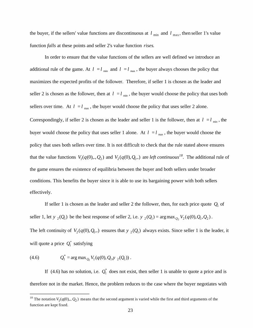
the buyer, if the sellers' value functions are discontinuous at minλ and maxλ , then seller 1's value

function falls at these points and seller 2's value function rises.

In order to ensure that the value functions of the sellers are well defined we introduce an

additional rule of the game. At minλλ = and maxλλ = , the buyer always chooses the policy that

maximizes the expected profits of the follower. Therefore, if seller 1 is chosen as the leader and

seller 2 is chosen as the follower, then at minλλ = , the buyer would choose the policy that uses both

sellers over time. At maxλλ = , the buyer would choose the policy that uses seller 2 alone.

Correspondingly, if seller 2 is chosen as the leader and seller 1 is the follower, then at minλλ = , the

buyer would choose the policy that uses seller 1 alone. At maxλλ = , the buyer would choose the

policy that uses both sellers over time. It is not difficult to check that the rule stated above ensures

that the value functions )),.,0(( 21 QqV and ,.)),0(( 12 QqV are left continuous18. The additional rule of

the game ensures the existence of equilibria between the buyer and both sellers under broader

conditions. This benefits the buyer since it is able to use its bargaining power with both sellers

effectively.

If seller 1 is chosen as the leader and seller 2 the follower, then, for each price quote 1Q of

seller 1, let )( 12 Qψ be the best response of seller 2, i.e. ),),0((maxarg)( 21212 2QQqVQ Q=ψ .

The left continuity of ,.)),0(( 12 QqV ensures that )( 12 Qψ always exists. Since seller 1 is the leader, it

will quote a price *1Q satisfying

(4.6) ))(,),0((maxarg 1211*1 1

QQqVQ Q ψ= .

If (4.6) has no solution, i.e. *1Q does not exist, then seller 1 is unable to quote a price and is

therefore not in the market. Hence, the problem reduces to the case where the buyer negotiates with

18 The notation )),.,0(( 21 QqV means that the second argument is varied while the first and third arguments of the function are kept fixed.

24

only a single seller, i.e. seller 2 in the foreign market. This provides additional motivation for our

detailed consideration of the one-seller scenario earlier in the section. Similarly, if seller 2 is chosen

as the leader and seller 1 the follower, then for each price quote 2Q of seller 2, let )( 21 Qψ be the

best response of seller 1, i.e. ),),0((maxarg)( 21121 1QQqVQ Q=ψ . The left continuity of

)),.,0(( 21 QqV ensures that )( 21 Qψ exists. Since seller 2 is the leader, it will quote a price *2Q

satisfying

(4.7) )),(),0((maxarg 2212*2 2

QQqVQ Q ψ= .

If *2Q does not exist, seller 2 is unable to quote a price so that seller 1 is the only seller in the market

and we are again in the single seller scenario discussed earlier. The buyer will choose seller 1 (seller

2) as the leader and seller 2 (seller 1) as the follower in equilibrium if and only if

)),(),0(()())(,),0(( *2

*21

*12

*1 QQqVQQqV ψψ <> .

Equilibria between the Buyer and Sellers

We can now state the following result that provides sufficient conditions for both sellers to

co-exist in any possible equilibrium with the buyer or for either seller to capture the market.

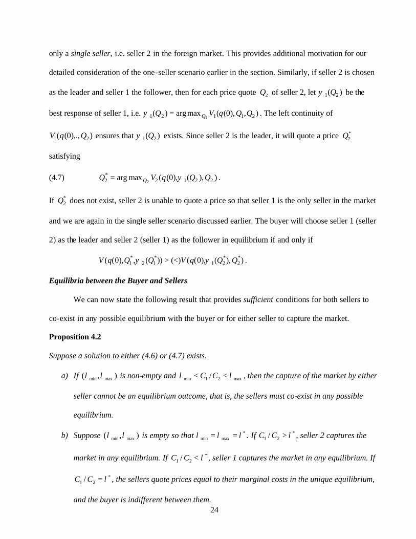
Proposition 4.2

Suppose a solution to either (4.6) or (4.7) exists.

a) If ),( maxmin λλ is non-empty and max21min / λλ << CC , then the capture of the market by either

seller cannot be an equilibrium outcome, that is, the sellers must co-exist in any possible

equilibrium.

b) Suppose ),( maxmin λλ is empty so that *maxmin λλλ == . If *

21 / λ>CC , seller 2 captures the

market in any equilibrium. If *21 / λ<CC , seller 1 captures the market in any equilibrium. If

*21 / λ=CC , the sellers quote prices equal to their marginal costs in the unique equilibrium,

and the buyer is indifferent between them.

25


The above proposition provides a precise connection between the analysis of the optimal

policies of the buyer presented in the previous sections and the equilibrium analysis of the present

section. We argued previously that the non-emptiness of the switching region ),( maxmin λλ is a

necessary but not sufficient condition for both sellers to co-exist in any possible equilibrium with the

buyer. For the sellers to co-exist in equilibrium with the buyer, the ratio of the prices they quote must

lie in the interval ),( maxmin λλ . The result of Proposition 4.2 a) says that if the costs of the sellers are

"aligned" so that their ratio lies within ),( maxmin λλ , then the ratio of the prices they quote in

equilibrium must also lie within ),( maxmin λλ . On the other hand, if ),( maxmin λλ is empty, then the

seller with the higher bargaining power (depending on whether *21 / λ>CC or *

21 / λ<CC ) captures

the market. However, as the following elementary result (whose proof we omit) shows, the level of

prices when seller 1 captures the market may be very different from the level when seller 2 captures

it.

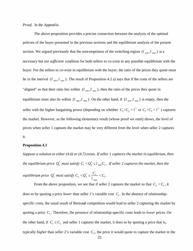
Proposition 4.3

Suppose a solution to either (4.6) or (4.7) exists. If seller 1 captures the market in equilibrium, then the equilibrium price *

1Q must satisfy 2min*11 CQC λ≤< . If seller 2 captures the market, then the

equilibrium price *2Q must satisfy 1

max

1*22 C

CQC <≤<

λ.

From the above proposition, we see that if seller 2 captures the market so that 12 CC < , it

does so by quoting a price lower than seller 1’s variable cost 1C . In the absence of relationship-

specific costs, the usual result of Bertrand competition would lead to seller 2 capturing the market by

quoting a price 1C . Therefore, the presence of relationship-specific costs leads to lower prices. On

the other hand, if 21 CC ≤ and seller 1 captures the market, it does so by quoting a price that is,

typically higher than seller 2’s variable cost 2C , the price it would quote to capture the market in the

26

absence of relationship-specific costs. Therefore, relationship-specific costs may either raise or

lower the level of prices depending on which seller captures the market.

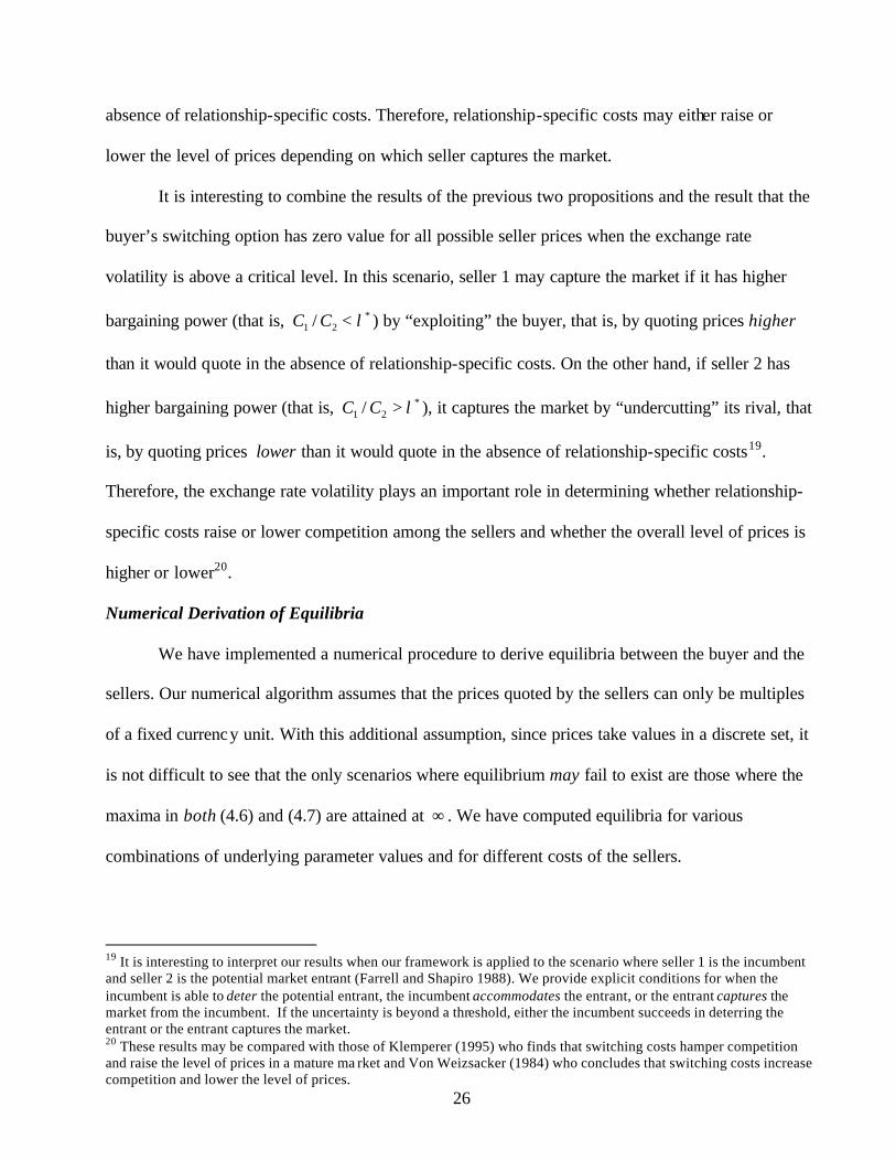
It is interesting to combine the results of the previous two propositions and the result that the

buyer’s switching option has zero value for all possible seller prices when the exchange rate

volatility is above a critical level. In this scenario, seller 1 may capture the market if it has higher

bargaining power (that is, *21 / λ<CC ) by “exploiting” the buyer, that is, by quoting prices higher

than it would quote in the absence of relationship-specific costs. On the other hand, if seller 2 has

higher bargaining power (that is, *21 / λ>CC ), it captures the market by “undercutting” its rival, that

is, by quoting prices lower than it would quote in the absence of relationship-specific costs19.

Therefore, the exchange rate volatility plays an important role in determining whether relationship-

specific costs raise or lower competition among the sellers and whether the overall level of prices is

higher or lower20.

Numerical Derivation of Equilibria

We have implemented a numerical procedure to derive equilibria between the buyer and the

sellers. Our numerical algorithm assumes that the prices quoted by the sellers can only be multiples

of a fixed currency unit. With this additional assumption, since prices take values in a discrete set, it

is not difficult to see that the only scenarios where equilibrium may fail to exist are those where the

maxima in both (4.6) and (4.7) are attained at ∞ . We have computed equilibria for various

combinations of underlying parameter values and for different costs of the sellers.

19 It is interesting to interpret our results when our framework is applied to the scenario where seller 1 is the incumbent and seller 2 is the potential market entrant (Farrell and Shapiro 1988). We provide explicit conditions for when the incumbent is able to deter the potential entrant, the incumbent accommodates the entrant, or the entrant captures the market from the incumbent. If the uncertainty is beyond a threshold, either the incumbent succeeds in deterring the entrant or the entrant captures the market. 20 These results may be compared with those of Klemperer (1995) who finds that switching costs hamper competition and raise the level of prices in a mature ma rket and Von Weizsacker (1984) who concludes that switching costs increase competition and lower the level of prices.

27

Equilibria with Cost Differentials

Figure 5 shows the variation of the equilibrium prices quoted by the sellers with the ratio of

the costs of the two sellers. The figure depicts all the three types of equilibria between the buyer and

the sellers: the region where seller 1 captures the market, an intermediate region where the sellers

co-exist when the costs are comparable and a third region where seller 2 captures the market.

Consistent with the result of Proposition 4.2, we note that both sellers co-exist when

max21min 09.1/04.1 λλ =<<= CC . However, as the figure indicates, the sellers may co-exist in

equilibrium even when 21 / CC does not lie in ),( maxmin λλ since the condition of Proposition 4.2 is a

sufficient but not necessary condition for co-existence. We notice that the level of prices quoted by

seller 1 when it captures the market is higher than the level of prices quoted by seller 2 when it

captures the market. This is consistent with the result of Proposition 4.3.

Figure 6 illustrates a scenario where the parameters chosen satisfy the condition (4.3).

Therefore, by the result of Proposition 4.1, in the monopolistic situation with a single seller, the

buyer would not enter the foreign market. When there are two potential sellers, the figure indicates

that there may be four possible outcomes: either seller capturing the market, both sellers co-existing

and, most interestingly, an intermediate region (where the costs of the two sellers are “close” to each

other) where the sellers quote infinite prices so that the buyer will not enter the foreign market. The

existence of equilibria with both sellers clearly shows that the buyer may enter the foreign market

when it negotiates with both sellers, that it would not otherwise have entered if it had negotiated with

only one seller. Interestingly, the equilibrium outcome may well be the capture of the market by

either seller. However, if the sellers’ costs are “close” to each other, the buyer enters the foreign

market only if there is an exogenously imposed ceiling on seller prices due to the possibility of

unrestrained tacit collusion between the sellers where the sellers prefer to accommodate each other

28

in equilibrium by quoting increasingly higher prices21. Thus, the intervention of a regulator may be

required to ensure that the buyer enters the foreign market.

Strategic Relationships with Relationship-Specific Costs and Exchange Rate Uncertainty

We will now combine all the results we have obtained to describe the effects of the interplay

between exchange rate uncertainty and differing relationship-specific costs on the strategic

relationships between the respective players.

First consider the monopolistic situation with a single seller. In the absence of exchange rate

uncertainty, we may see that if a trading equilibrium exists (conditional on the seller’s cost), the

seller quotes the monopoly price at which the buyer’s profits are zero. The seller, however, obtains

positive profits in general. In the presence of exchange rate uncertainty, the buyer and the seller both

possess “values of waiting” to enter into business. If the uncertainty is “low” (that is, condition (4.2)

of Proposition 4.1 holds), then equilibrium exists where, in general, both the buyer and the seller

obtain positive expected profits. However, if the uncertainty is “high” (that is, condition (4.3) of

Proposition 4.1 holds), the seller is never satiated at a finite price and the buyer will not enter the

foreign market unless there is an exogenously imposed ceiling on the prices the seller may quote.

Now consider the scenario where the buyer negotiates with both sellers. In the absence of

exchange rate uncertainty, we may see that the seller with the more favorable combination of its

variable costs and buyer relationship-specific costs, captures the market. In the presence of “low”

uncertainty (that is, (4.2) holds), we may have equilibria where either seller captures the market or

both sellers co-exist (as Figure 5 indicates) depending on the relative magnitudes of their respective

costs and the relationship-specific costs of the buyer. However, if the costs of the sellers are

“aligned” as in the hypothesis of Proposition 4.2, the sellers must co-exist in equilibrium with the

21 Therefore, one of the equilibrium outcomes may be tacit collusion. Farrell and Shapiro (1988) and Klemperer (1987a) both report the possibility of tacit collusion in markets with switching costs in frameworks where sellers compete in each period. We show that tacit collusion may occur with long-term contracts between buyers and sellers.

29

buyer. Therefore, the presence of relationship-specific costs and exogenous uncertainty may allow

both sellers to co-exist in equilibrium.

Finally, consider the situation where the exchange rate uncertainty is “high” (that is, (4.3)

holds). When the relationship-specific costs of the buyer vis-à-vis the sellers are different, the

switching option of the buyer may have positive value provided the exchange rate volatility is below

the critical threshold (Proposition 3.2) above which the buyer’s switching option has zero value. In

general, either seller may be able to quote a price that captures the market or both may choose to

quote prices in equilibrium that allow their co-existence. If the sellers’ costs are identical or very

“close” to each other, the market capture price for either seller, if one exists, would be very close to

its cost so that the seller would obtain low expected profits from capturing the market. The presence

of high uncertainty may therefore induce both sellers to accommodate each other wherein they quote

prices that allow their co-existence. However, very high uncertainty levels may induce both sellers to

quote increasingly higher prices thereby delaying the buyer’s entry into the market, but obtaining

higher profits when in business and this may lead to unrestrained tacit collusion by the sellers.

Hence, the buyer may not enter the foreign market when the sellers’ costs are “close” to each other

with differing relationship-specific costs as seen in Figure 6. The entry of the buyer is possible only

if a regulator imposes a price ceiling on the sellers.

If the sellers' costs are significantly different from each other and the buyer relationship-

specific costs are different, we may have equilibria where either seller captures the market or both

sellers co-exist even with high exchange rate volatilities as illustrated in Figure 6. However, as

Proposition 3.2 and Figures 4a, 4b, 4c illustrate, above the critical volatility level where the buyer’s

switching option has zero value, both sellers cannot co-exist in equilibrium regardless of their costs.

By the results of part b) of Proposition 4.2 and Proposition 4.3, seller 1 captures the market if it has

higher bargaining power by quoting a price that is typically higher than it would quote without

30

relationship-specific costs. On the other hand, if seller 2 has higher bargaining power, it captures the

market by quoting a price that is lower than it would quote without relationship-specific costs.

Therefore, the presence of relationship-specific costs and exogenous dynamic uncertainty

may either increase or decrease competition among the sellers and either increase or decrease the

level of prices. The complexity of the equilibrium dynamics between the buyer and the sellers

described above indicates that the presence of both differing relationship-specific costs and

exogenous uncertainty, causes very significant changes in the strategic relationships between the

respective players.

5. Summary and Conclusions

In this paper, we have proposed and investigated an equilibrium framework to analyze

strategic relationships between buyers and sellers in different countries exposed to exchange rate

uncertainty. An investigation of this scenario is particularly relevant due to the dramatic acceleration

in globalization over the past decade. Our objective was to analyze the impact of differences in the

relationship-specific costs of the buyers and exchange rate uncertainty on the relative bargaining

power of the respective players and the resulting effect on the nature of their strategic relationships.

We showed that the presence of relationship-specific costs may lead to various possible

equilibrium outcomes: switching equilibria where the sellers co-exist, no-switching equilibria where

either seller may capture the market, or tacit collusion between the sellers that may necessitate the

imposition of price ceilings to induce the entry of the buyer. The level of exchange rate uncertainty

plays a crucial role in determining the actual equilibrium outcome. Contrary to the extant literature,

we find that, in the presence of exchange rate uncertainty, relationship-specific costs may either raise

or lower competition and either raise or lower the level of prices in a mature market.

31

As mentioned in Section 2 (footnote 15), we may modify our framework to consider the

situation where the buyer, after exiting the foreign market from a relationship with either seller, must

renegotiate with both sellers before re-entering the market. The prices the sellers quote are constant

(in their currency) between successive renegotiations. For tractability, we may make alternative

simplifying assumptions.

One alternative is to assume that the buyer is myopic, that is, after each renegotiation, the

buyer responds to the sellers’ quoted prices by adopting a policy that maximizes its expected profits

till it exits the market without considering the profits it may derive as a result of future re-entries into

the market. Hence, each “round” of the renegotiation game is independent of other rounds. This may

be a reasonable description of the behavior of a buyer contemplating trade with foreign sellers where

the buyer’s relevant decision horizon ends at the time it exits the foreign market. The renegotiations

may occur at different values of the exchange rate that may be exogenously specified or

endogenously determined. After each renegotiation, the buyer adopts an entry, exit, and switching

policy assuming that it will not re-enter the foreign market once it has exited it. The sellers quote

prices rationally anticipating the buyer’s myopic policy. Each round of this renegotiation game is

now a straightforward modification of our existing framework to the scenario where the buyer does

not re-enter the foreign market after exiting it (see footnote 16). We can then show that the results of

this paper qualitatively apply to each round of this renegotiation game where the notions of market

capture and co-existence pertain to each round. The sellers’ quoted prices may now differ across

rounds of the game depending on the exchange rate levels at which renegotiation occurs.

Another alternative is to replace the assumption that the buyer is myopic with the assumption

that renegotiations may occur only when the exchange rate has a specific value. The value of the

exchange rate at which renegotiations may occur can be exogenous or can be chosen by the buyer.

This may be a reasonable description of the behavior of a buyer that contemplates entering a foreign

32

market and negotiates with foreign sellers only when the exchange rate is at a favorable level. For

example, once a buyer has exited a foreign market because the exchange rate is unfavorable, it is

reasonable to suppose that the buyer will contemplate re-entry and renegotiate with foreign sellers

only when the exchange rate returns to a favorable level. It may easily be seen, given the process

(2.1) for the exchange rate, that equilibria of this repeated game are renegotiation-proof, that is,

sellers quote constant prices in their currency that are never renegotiated. Our main results are not

qualitatively affected by this modification of our framework although the equilibrium prices the

sellers quote in this game are, in general, different from the equilibrium prices we obtain within the

framework assumed in this paper.

As discussed in the introduction (footnote 2), our model is applicable to other economic

scenarios. In this paper, we have considered the scenario where the buyer's profits are influenced by

the stochastic variation of its costs due to the sellers. It is easy to modify our model to investigate

economic scenarios where the costs are constant while the payoffs are stochastic. Such a model may

be appropriate in the investigation of the strategic behavior of a buyer that is investing in new

technology, incurring expenditure on research and development, training human capital, developing

natural resources, etc. In each case, the buyer may choose to dynamically incur different levels of

sunk costs (analogous to the "relationship specific" costs in our model) to obtain proportionally

higher random payoffs.

Several important issues can be considered in future research. We may easily extend our

framework to cons ider non-identical buyers, that is, different buyers may have different pairs of

relationship-specific costs vis-à-vis the sellers that may be unobservable to the sellers (see footnote

12). We can also include the possibility of new buyers entering the market periodically with the

sellers quoting different prices to new buyers (see, for example, Klemperer 1995, Farrell and Shapiro

1988). It would be interesting to consider the general dynamic game between the buyer and the

33

sellers where each seller may periodically change the price it quotes in response to actions by the

buyer and by the other seller. It would also be important to examine the influence of information

asymmetry amongst the players on the existence and nature of the equilibria between them.

References

Adler, M. and B. Dumas (1983). “International Portfolio Choice and Corporation Finance: A Synthesis,” Journal of Finance, 38(3), 925-984. Beggs, A. and P. Klemperer (1992). “Multiperiod Competition with Switching Costs,” Econometrica, 60, 651-666. Carlton, D. (1986). “The Rigidity of Prices,” The American Economic Review, 76, 637-658. Dixit, A. (1989). “Entry and Exit Decisions under Uncertainty,” Journal of Political Economy, 97(3), 620-638. Dixit, A. (1991). “Irreversible Investment with Price Ceilings,” Journal of Political Economy, 99, 541-557. Dixit, A. and R. Pindyck. (1994). Investment under Uncertainty. Princeton: Princeton University Press. Farrell, J. and C. Shapiro (1988). “Dynamic Competition with Switching Costs,” RAND Journal of Economics, 19, 123-137. Farrell, J. and C. Shapiro (1989). “Optimal Contracts with Lock-In,” The American Economic Review, 79(1), 51-68. Froot, K. (1993). “Foreign Direct Investment,” NBER Project Report, University of Chicago Press. Froot, K. and P. Klemperer (1989). “Exchange Rate Pass-Through when Market Share Matters,” The American Economic Review, 79(4), 637-654. Grenadier, S. (2000). Game Choices: The Intersection of Real Options and Game Theory, Risk Books. Huisman, K. (2001). Technology Investment: A Game Theoretic Real Options Approach, Kluwer Academic Publishing. Joskow, P. (1987). “Contract Duration and Relationship-Specific Investments: Empirical Evidence from Coal Markets,” The American Economic Review, 77(1), 168-185.

34

Klemperer, P. (1987a). “Markets with Consumer Switching Costs,” The Quarterly Journal of Economics, 102(2), 375-394. Klemperer, P. (1987b). “The Competitiveness of Markets with Consumer Switching Costs,” RAND Journal of Economics, 18, 138-150. Klemperer, P. (1995). “Competition when Consumers have Switching Costs: An Overview with Applications to Industrial Organization, Macroeconomics and International Trade,” Review of Economic Studies, 62(4), 515-539. MacLeod, B. and J. Malcomson (1993). “Investments, Holdup, and the Form of Market Contracts,” The American Economic Review, 83(4), 811-837. Padilla, A.J. (1995). “Revisiting Dynamic Duopoly with Consumer Switching Costs,” Journal of Economic Theory, 67(2), 520-530. Trigeorgis, L. (1996). Real Options, Managerial Flexibility and Strategy in Resource Allocation, MIT Press. Tirole, J. (1988). The Theory of Industrial Organization, MIT Press. Von Weizsacker, C. (1984). “The Costs of Substitution,” Econometrica, 52(5), 1085-1116. Worldwatch Institute (2002). “Globalization Straining Planet’s Health,” News Release.

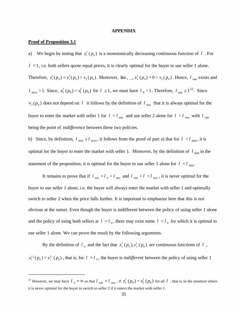
35

APPENDIX

Proof of Proposition 3.1

a) We begin by noting that )( 01 pz λ is a monotonically decreasing continuous function of λ . For

1=λ , i.e. both sellers quote equal prices, it is clearly optimal for the buyer to use seller 1 alone.

Therefore, )()()( 020110

11 pvpvpz >= . Moreover, )(0)(lim 0201 pvpz <=∞→

λλ . Hence, maxλ exists and

1max >λ . Since, )()( 0101 pvpz λλ = for 1≤λ , we must have 10 >λ . Therefore, 1min ≥λ 22. Since

)( 02 pv does not depend on λ it follows by the definition of maxλ that it is always optimal for the

buyer to enter the market with seller 1 for maxλλ < and use seller 2 alone for maxλλ > with maxλ

being the point of indifference between these two policies.

b) Since, by definition, maxmin λλ ≤ , it follows from the proof of part a) that for minλλ < , it is

optimal for the buyer to enter the market with seller 1. Moreover, by the definition of minλ in the

statement of the proposition, it is optimal for the buyer to use seller 1 alone for minλλ < .

It remains to prove that if max0min λλλ <= and maxmin λλλ << , it is never optimal for the

buyer to use seller 1 alone, i.e. the buyer will always enter the market with seller 1 and optimally

switch to seller 2 when the price falls further. It is important to emphasize here that this is not

obvious at the outset. Even though the buyer is indifferent between the policy of using seller 1 alone

and the policy of using both sellers at 0λλ = , there may exist some 0λλ > for which it is optimal to

use seller 1 alone. We can prove the result by the following arguments.

By the definition of 0λ and the fact that )(),( 0101 pvpz λλ are continuous functions of λ ,

)()( 010100 pvpz λλ = , that is, for 0λλ = , the buyer is indifferent between the policy of using seller 1

22 However, we may have ∞=0λ so that maxmin λλ = , if )()( 0101 pvpz λλ = for all λ , that is, in the situation where

it is never optimal for the buyer to switch to seller 2 if it enters the market with seller 1.

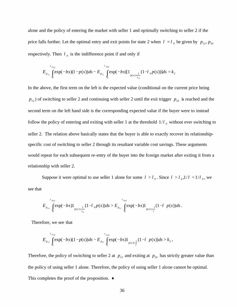
36

alone and the policy of entering the market with seller 1 and optimally switching to seller 2 if the

price falls further. Let the optimal entry and exit points for state 2 when 0λλ = be given by 2012 , pp

respectively. Then 0λ is the indifference point if and only if

200

1)(

0

))](1(1)[exp())(1)(exp(20

0

12

20

12kdsspsEdsspsE

pp

sppp =−−−−− ∫∫ ≤

λββτ

λ

τ

In the above, the first term on the left is the expected value (conditional on the current price being

12p ) of switching to seller 2 and continuing with seller 2 until the exit trigger 20p is reached and the

second term on the left hand side is the corresponding expected value if the buyer were to instead

follow the policy of entering and exiting with seller 1 at the threshold 0/1 λ without ever switching to

seller 2. The relation above basically states that the buyer is able to exactly recover its relationship-

specific cost of switching to seller 2 through its resultant variable cost savings. These arguments

would repeat for each subsequent re-entry of the buyer into the foreign market after exiting it from a

relationship with seller 2.

Suppose it were optimal to use seller 1 alone for some 0λλ > . Since 00 /1/1, λλλλ <> , we

see that

dsspsEdsspsEpp

spp

spp ))(1(1)exp())(1(1)exp(

20

12

20

0

12

01

)(0

01

)(λβλβ

τ

λ

τ

λ∫∫ −−>−−

≤≤.

Therefore, we see that

20

1)(0

))(1(1)exp())(1)(exp(20

12

20

12kdsspsEdsspsE

pp

sppp >−−−−− ∫∫ ≤λββ

τ

λ

τ

,

Therefore, the policy of switching to seller 2 at 12p and exiting at 20p has strictly greater value than

the policy of using seller 1 alone. Therefore, the policy of using seller 1 alone cannot be optimal.

This completes the proof of the proposition. ♦

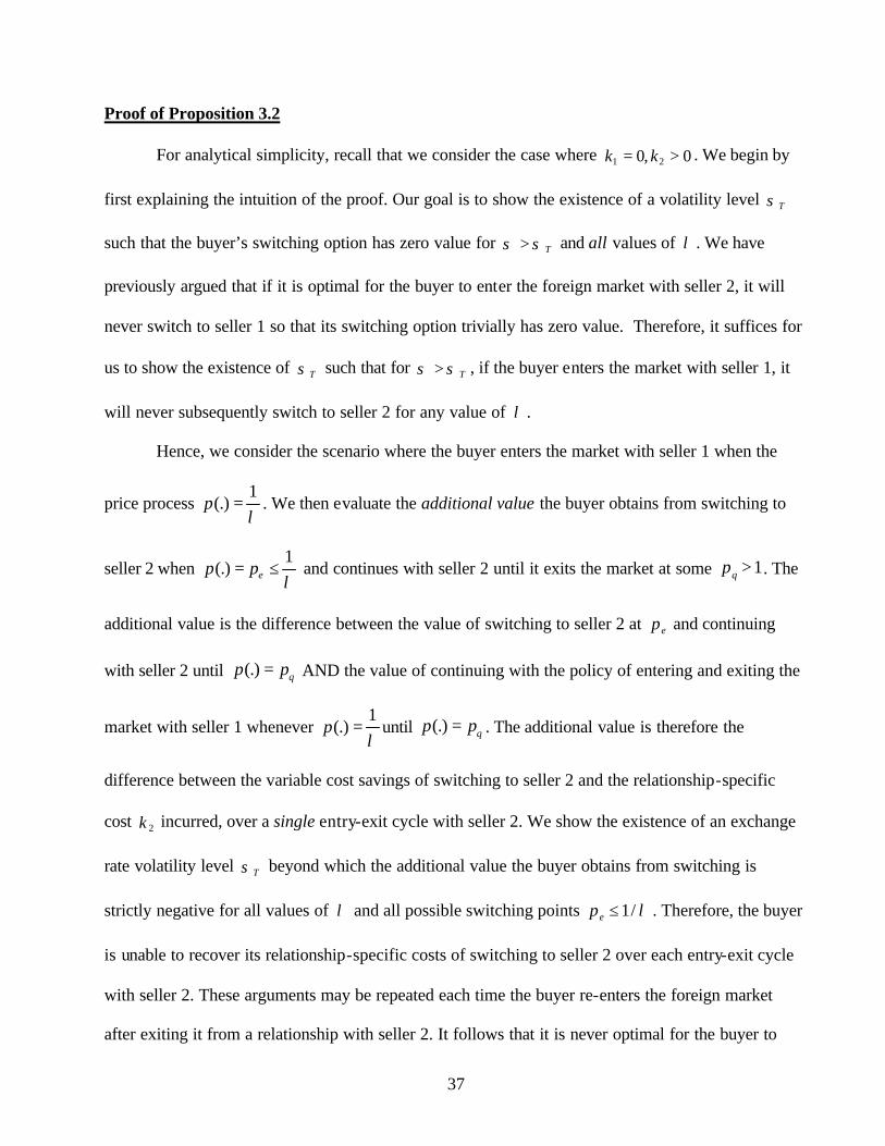
37


For analytical simplicity, recall that we consider the case where 0,0 21 >= kk . We begin by

first explaining the intuition of the proof. Our goal is to show the existence of a volatility level Tσ

such that the buyer’s switching option has zero value for Tσσ > and all values of λ . We have

previously argued that if it is optimal for the buyer to enter the foreign market with seller 2, it will

never switch to seller 1 so that its switching option trivially has zero value. Therefore, it suffices for

us to show the existence of Tσ such that for Tσσ > , if the buyer enters the market with seller 1, it

will never subsequently switch to seller 2 for any value of λ .

Hence, we consider the scenario where the buyer enters the market with seller 1 when the

price process λ1

(.) =p . We then evaluate the additional value the buyer obtains from switching to

seller 2 when λ1

(.) ≤= epp and continues with seller 2 until it exits the market at some 1>qp . The

additional value is the difference between the value of switching to seller 2 at ep and continuing

with seller 2 until qpp =(.) AND the value of continuing with the policy of entering and exiting the

market with seller 1 whenever λ1

(.) =p until qpp =(.) . The additional value is therefore the

difference between the variable cost savings of switching to seller 2 and the relationship-specific

cost 2k incurred, over a single entry-exit cycle with seller 2. We show the existence of an exchange

rate volatility level Tσ beyond which the additional value the buyer obtains from switching is

strictly negative for all values of λ and all possible switching points λ/1≤ep . Therefore, the buyer

is unable to recover its relationship-specific costs of switching to seller 2 over each entry-exit cycle

with seller 2. These arguments may be repeated each time the buyer re-enters the foreign market

after exiting it from a relationship with seller 2. It follows that it is never optimal for the buyer to

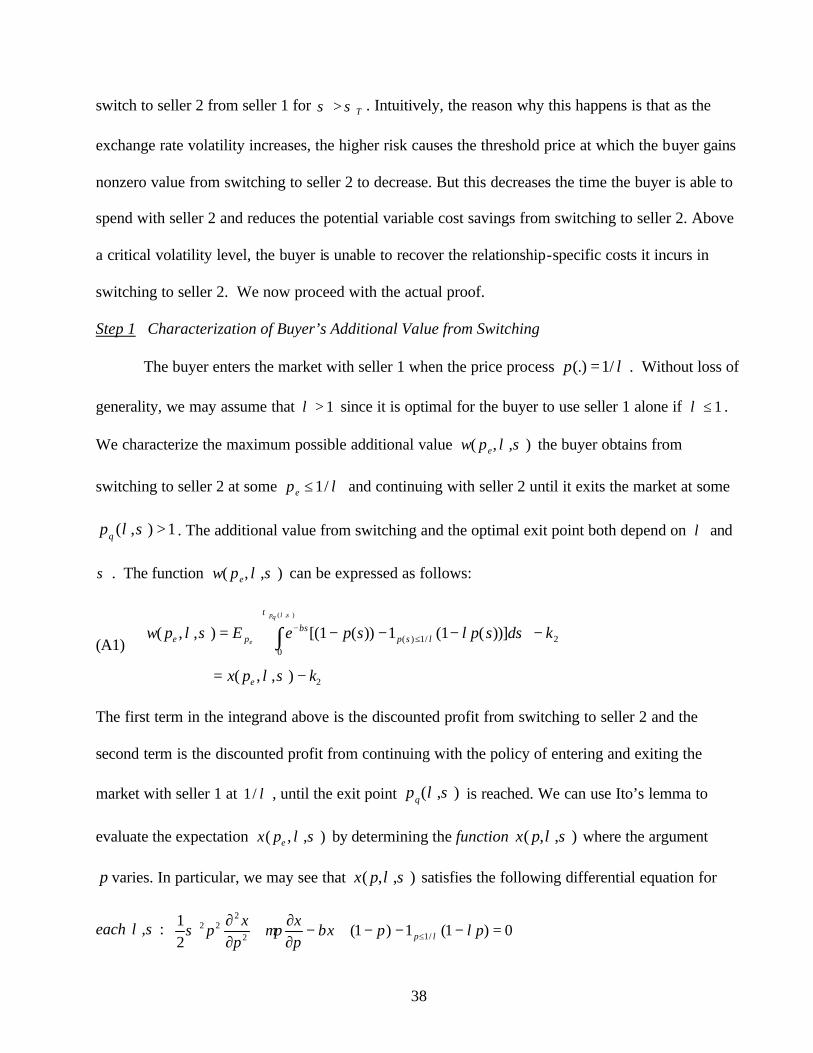
38

switch to seller 2 from seller 1 for Tσσ > . Intuitively, the reason why this happens is that as the

exchange rate volatility increases, the higher risk causes the threshold price at which the buyer gains

nonzero value from switching to seller 2 to decrease. But this decreases the time the buyer is able to

spend with seller 2 and reduces the potential variable cost savings from switching to seller 2. Above

a critical volatility level, the buyer is unable to recover the relationship-specific costs it incurs in

switching to seller 2. We now proceed with the actual proof.

Step 1 Characterization of Buyer’s Additional Value from Switching

The buyer enters the market with seller 1 when the price process λ/1(.) =p . Without loss of

generality, we may assume that 1>λ since it is optimal for the buyer to use seller 1 alone if 1≤λ .

We characterize the maximum possible additional value ),,( σλepw the buyer obtains from

switching to seller 2 at some λ/1≤ep and continuing with seller 2 until it exits the market at some

1),( >σλqp . The additional value from switching and the optimal exit point both depend on λ and

σ . The function ),,( σλepw can be expressed as follows:

(A1)

2

20

/1)(

),,(

))](1(1))(1[(),,(),(

kpx

kdsspspeEpw

e

sps

pe

qp

e

−=

−

−−−= ∫ ≤−

σλ

λσλσλτ

λβ

The first term in the integrand above is the discounted profit from switching to seller 2 and the

second term is the discounted profit from continuing with the policy of entering and exiting the

market with seller 1 at λ/1 , until the exit point ),( σλqp is reached. We can use Ito’s lemma to

evaluate the expectation ),,( σλepx by determining the function ),,( σλpx where the argument

p varies. In particular, we may see that ),,( σλpx satisfies the following differential equation for

each σλ , : 0)1(1)1(21

/12

222 =−−−+−

∂∂

+∂∂

≤ ppxpx

pp

xp p λβµσ λ

39

with the boundary conditions 0|),,(

,0),),,(( ),( =∂

∂= = σλ

σλσλσλ

qppq ppx

px . These arise from the fact

that ),,( σλpx attains its maximum possible value at ),( σλqpp = . From the above, we see that

),,( σλpx has the following functional form:

(A2)

),(for ; 0

),(/1for ;1

),(),(

/1for ;)1(

),(),,(

)()(

)(

11

1

σλ

σλλµββ

σλσλ

λµβ

λσλσλ

σηση

ση

q

q

pp

ppp

pCpB

pp

pApx

≥=

<≤−

−++=

<−−

+=

−+

+

In the above, )(),( 11 σηση −+ are the positive and negative roots of the quadratic equation (2.13)

where we have indicated their explicit dependence on the exchange rate volatility σ .

Step 2 Coefficients and Exit Point ),( σλqp

The coefficients above and the exit point ),( σλqp are obtained from value matching

(continuity) and smooth pasting (differentiability) conditions at the boundaries of the different

regions. We omit writing down these equations for the sake of notational brevity. We can solve these

equations after some tedious algebra to obtain the following equation for ),( σλqp :

(A3) )()())(1)(,()),()()(( 11)(

11 σηβµσησλβσλλβσµη ση +++ −=−+−−

qq pp

It is not difficult to check that there is exactly one root of the above equation that is greater than 1

and this is the required exit point.

Step 3 Properties of roots )(),( 11 σηση −+ and coefficients ),(),,( σλσλ BA

The coefficients ),(),,( σλσλ AB in (A2) are given by

(A4)

))(

)((

))()((),(),(

)),(())()()((

)(1)),((

))()(()(

),(

1

11

)(

)(1

11

1)(

11

1

1

11

µβββσµη

σησηλ

σλσλ

σλσησηµβ

σησλ

σησηβση

σλ

ση

σηση

−−

−+=

−−−

+−

=

−

−+

−−+

−−

−+

−

+

++

BA

ppB qq

40

We may easily check that the roots )(),( 11 σηση −+ of equation (2.13) have the following properties:

(A5) 0)(lim,1)(lim ,0)(,1)( 1111 ==<> −∞→

+∞→

−+ σησησηση σσ

From (A4) we see that

(A6) |)),((||))()()((

)(1||)),((||

))()(()(

||),(| )(1

11

1)(

11

1 11 σηση σλσησηµβ

σησλ

σησηβση

σλ++ −

−+

−−

−+

−

−−−

+−

≤ qq ppB

Since 1 and 1),( >> λσλqp and 1)(1 >+ ση , we see that 1)),(( and 1)),(( )(1)( 11 <<

++ −− σηση σλσλ qq pp .

Hence, from (A5) and (A6), we see that

(A7) µβ

σλσ −≤∞→

1|),(|lim B

where the inequality above holds uniformly in λ . We now see from (A1), (A2), (A4), (A5), (A7),

0)1(

)()1(

)1()

)()(

())()((

)())(,(lim

)1())(,(lim),,(lim),,(lim

2

21

11

)()(

2)(

2

11

1

<−−

−+

−−

=

−−

−+

−−

−+=

−−

−+=−=

−

−+∞→

∞→∞→∞→

++

+

kpp

kpp

pB

kp

pAkpxpw

ee

eee

eeee

µβλ

µβλ

µβλ

µβββσµη

σησηλ

σλ

µβλ

σλσλσλ

σηση

σ

σησσσ

Since λ1

≤ep so that 1≤epλ , we see that the inequality above holds uniformly in ]1,0[∈ep and

]1

,1[ep

∈λ . Since ),,( σλepw is a continuous function of its arguments, this clearly implies the

existence of an exchange rate volatility level Tσ beyond which the additional value of switching to

seller 2 from seller 1 is non-positive for all λ and all possible switching points λ/1≤ep . Since, as

we have noted earlier, it is sub-optimal for the buyer to switch to seller 1 after entering the market

with seller 2, it follows that the buyer’s switching option has zero value for Tσσ > . Therefore, for

Tσσ > , the buyer either only uses seller 1 or only seller 2 whenever it is in the foreign market. This

completes the proof. ♦

41


a) Without loss of generality, let us assume that the seller in the foreign market is seller 2. Given a

price quote 22 CQ ≥ of seller 2, the buyer’s long term stationary switching policies are to enter a

relationship with seller 2 when the price process (.)2qQ in the buyer’s currency hits a level 2ep and

to exit a relationship with seller 2 when the price process hits a level 2qp where 2

ep and 2qp depend

only on the sunk cost of using seller 2, i.e. 2k , the drift and volatility of the exchange rate process

and the buyer’s discount parameter β . Using standard dynamic programming arguments (see the

derivation of the value functions of the sellers in Section 4, especially equations (4.4) and (4.5)), we

may check that seller 2’s initial value function )(2 pV as a function of the initial price p in the

buyer's currency is given by

(A8) buyer the tosellsseller theand )0( if ))0((

idle isbuyer theand )0( if ))0(())0((

22'

222

22222

1

2

1

2

qQ

eQ

pqQCQ

qQD

pqQqQAqQV

<−

+=

≥=

+

−

βρ

ρ

where −+11 , ρρ are the positive and negative root of (2.13) with β replaced by 'β and the coefficients

above are determined by the following value matching conditions:

(A9) '

2222'

2222 1

2

1

2

1

2

1

2)()( ;)()(

ββρρρρ CQ

pDpACQ

pDpA qQqQeQeQ−

+=−

+=+−+−

From (A9), we easily see that

(A10) 0])()()()(

)()([

1111

11

2 2222

22

'22 >

−

−−= −+−+

++

ρρρρ

ρρ

βqeeq

eqQ

pppp

ppCQA since 22

eq pp >

The price quote *2Q is an equilibrium price if and only if seller 2’s value function is maximized at

*2Q , i.e. ))0((maxarg 22

*2 2

qQVQ Q= . From (A8), (A10), we see that

42

(A11) ]

)()()()(

)()([))0(())((lim

))0((lim))0((lim

1111

111

1

2

1

222

2222

22

2'22

222

−+−+

++−−

−

−

−−=

=

∞→

∞→∞→

ρρρρ

ρρρ

ρ

ρ

βqeeq

eqQ

QQQ

pppp

ppqQ

CQ

qQAqQV

])()()()(

)()([))0()(

)()((lim

1111

111

11

2 2222

22

'22

12

−+−+

++−

−−

−

−−=

+

∞→ ρρρρ

ρρρρρ

βqeeq

eqQ

pppp

ppq

QCQ

We now recall that −1ρ is the negative root of the equation 0

21

)21

( 222' =+−+− xxx σσµβ .

We see that 11 −>−ρ , i.e. –1 is less than both the roots of the above equation, if and only if the left

hand side above is positive when evaluated at 1−=x and this is exactly condition (4.3) of the

proposition. We therefore see that if (4.3) holds, 11 −>−ρ and we easily see from (A11) that

(A12) ∞=∞→ ))0((lim 222qQVQ

(A12) clearly implies that the seller is never satiated at a finite price so that the buyer will not enter

the foreign market. On the other hand, condition (4.2) is equivalent to 11 −<−ρ . In this case, it is

easy to see that equations (A8), (A9), (A11) imply that

0))0((lim))0((lim 2222 222== →∞→ qQVqQV CQQ

Since (.)2V is a continuous function, we see that its maximum exists and is attained at some *2Q

which is the required equilibrium price. Moreover, we can analytically determine the equilibrium

price *2Q from the explicit analytical expressions for (.)2V . Therefore, an equilibrium between the

buyer and the seller exists. This completes the proof of part a).

b) If there is an exogenously imposed ceiling ceilQ on seller prices, then the fact that ))0((2 qQV ceil is

finite clearly implies that the seller quotes a finite price in equilibrium that may be ceilQ if it is

sufficiently high. ♦

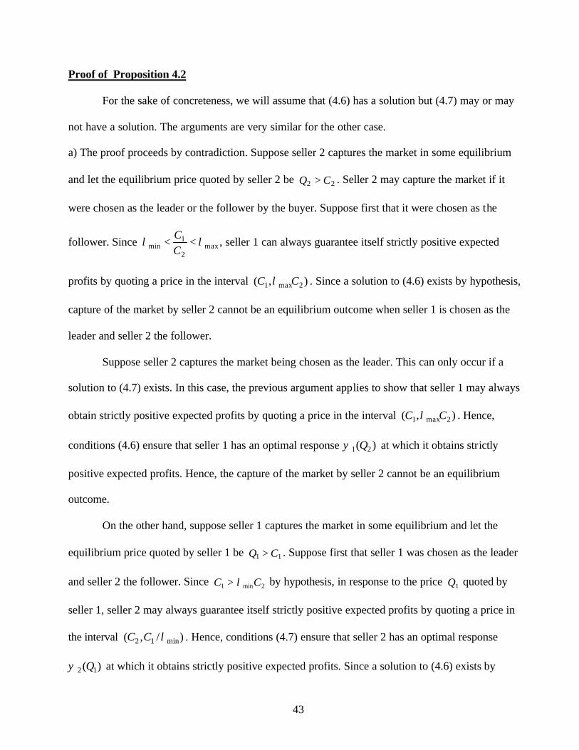
43


For the sake of concreteness, we will assume that (4.6) has a solution but (4.7) may or may

not have a solution. The arguments are very similar for the other case.

a) The proof proceeds by contradiction. Suppose seller 2 captures the market in some equilibrium

and let the equilibrium price quoted by seller 2 be 22 CQ > . Seller 2 may capture the market if it

were chosen as the leader or the follower by the buyer. Suppose first that it were chosen as the

follower. Since max2

1min λλ <<

CC

, seller 1 can always guarantee itself strictly positive expected

profits by quoting a price in the interval ),( 2max1 CC λ . Since a solution to (4.6) exists by hypothesis,

capture of the market by seller 2 cannot be an equilibrium outcome when seller 1 is chosen as the

leader and seller 2 the follower.

Suppose seller 2 captures the market being chosen as the leader. This can only occur if a

solution to (4.7) exists. In this case, the previous argument applies to show that seller 1 may always

obtain strictly positive expected profits by quoting a price in the interval ),( 2max1 CC λ . Hence,

conditions (4.6) ensure that seller 1 has an optimal response )( 21 Qψ at which it obtains strictly

positive expected profits. Hence, the capture of the market by seller 2 cannot be an equilibrium

outcome.

On the other hand, suppose seller 1 captures the market in some equilibrium and let the

equilibrium price quoted by seller 1 be 11 CQ > . Suppose first that seller 1 was chosen as the leader

and seller 2 the follower. Since 2min1 CC λ> by hypothesis, in response to the price 1Q quoted by

seller 1, seller 2 may always guarantee itself strictly positive expected profits by quoting a price in

the interval )/,( min12 λCC . Hence, conditions (4.7) ensure that seller 2 has an optimal response

)( 12 Qψ at which it obtains strictly positive expected profits. Since a solution to (4.6) exists by

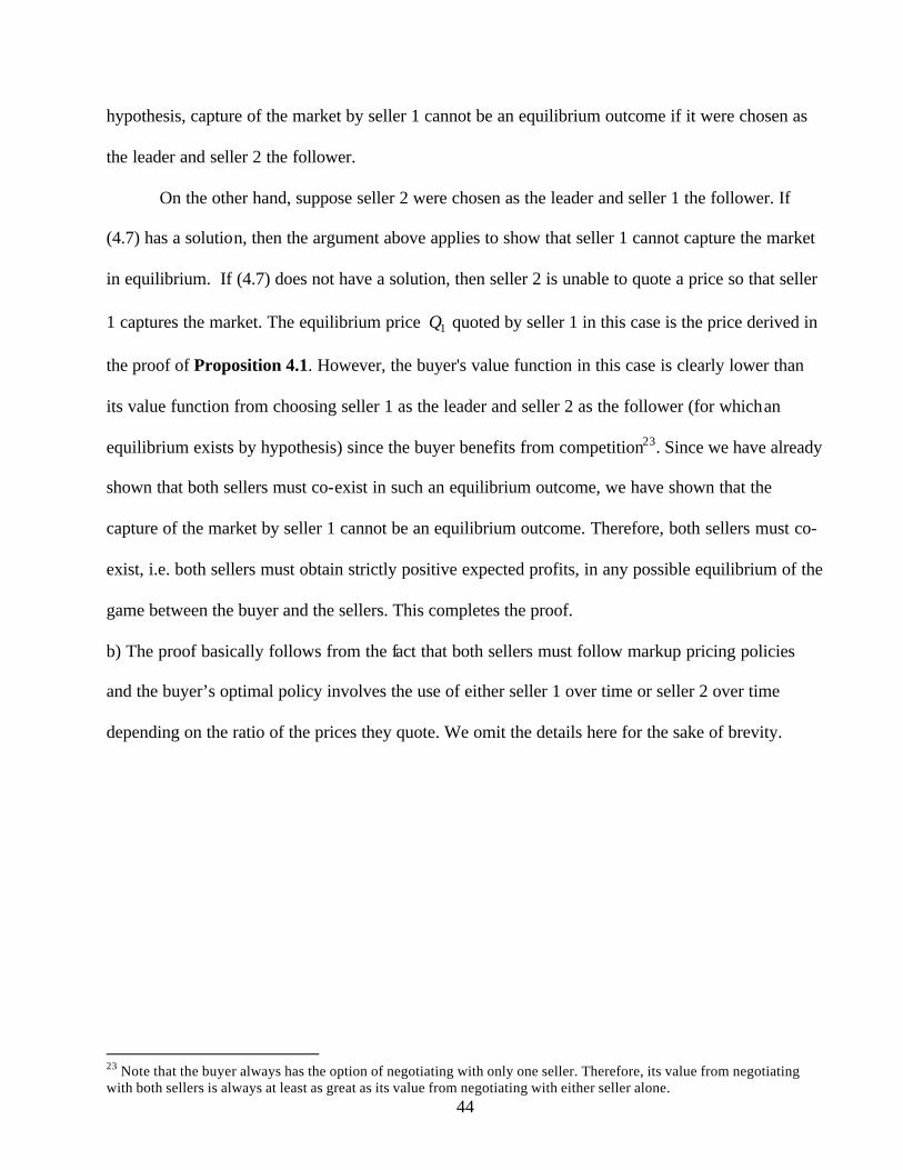
44

hypothesis, capture of the market by seller 1 cannot be an equilibrium outcome if it were chosen as

the leader and seller 2 the follower.

On the other hand, suppose seller 2 were chosen as the leader and seller 1 the follower. If

(4.7) has a solution, then the argument above applies to show that seller 1 cannot capture the market

in equilibrium. If (4.7) does not have a solution, then seller 2 is unable to quote a price so that seller

1 captures the market. The equilibrium price 1Q quoted by seller 1 in this case is the price derived in

the proof of Proposition 4.1. However, the buyer's value function in this case is clearly lower than

its value function from choosing seller 1 as the leader and seller 2 as the follower (for which an

equilibrium exists by hypothesis) since the buyer benefits from competition23. Since we have already

shown that both sellers must co-exist in such an equilibrium outcome, we have shown that the

capture of the market by seller 1 cannot be an equilibrium outcome. Therefore, both sellers must co-

exist, i.e. both sellers must obtain strictly positive expected profits, in any possible equilibrium of the

game between the buyer and the sellers. This completes the proof.

b) The proof basically follows from the fact that both sellers must follow markup pricing policies

and the buyer’s optimal policy involves the use of either seller 1 over time or seller 2 over time

depending on the ratio of the prices they quote. We omit the details here for the sake of brevity.

23 Note that the buyer always has the option of negotiating with only one seller. Therefore, its value from negotiating with both sellers is always at least as great as its value from negotiating with either seller alone.

Figure 1a (drift =0, beta = 0.025, initial price = 1.5, k1 = 0.01, k2 = 1.0, sigma = 0.1)

3.23.33.43.53.63.73.83.9

1.05 1.07 1.09 1.11 1.13 1.15 1.17 1.19

lambdaLambda_min = 1.05, Lambda_max = 1.13

Fir

m's

Val

ue

Fu

nct

ion

s

v

v1v2

Figure 1b (drift = 0, beta = 0.025, initial price = 1.5, k1 = 0.1, k2 =1.0, sigma = 0.1)

2.52.72.93.13.33.53.73.9

1.04 1.06 1.08 1.1 1.12 1.14

lambdaDegenerate Switching Region

Fir

m's

Val

ue

Fu

nct

ion

s

v

v1

v2

Figure 2a (mu = 0, beta = 0.025, k1 = 0.01, initial price = 1.5, sigma = 0.15, lambda = 1.1)

7

7.2

7.4

7.6

7.8

8

0.5 0.7 0.9 1.1 1.3 1.5

k2kmin = 0.5, kmax = 1.2

Fir

m V

alu

e F

un

ctio

ns

v

v1

v2

Figure 2b (mu = 0, beta = 0.025, k1 = 0.01, initial price =1.5, sigma = 0.15, lambda = 1.7)

3.5

4

4.5

5

5.5

5 6 7 8 9

k2Degenerate Switching Region

Firm

Val

ue F

unct

ions

vv1v2

Figure 3a (mu = 0, beta = 0.025, initial price = 1.5, k1 = 0.01, k2 = 1.0, sigma = 0.1)

0

0.5

1

1.5

1 1.05 1.1 1.15 1.2 1.25 1.3

lambdaLambda_min = 1.07, lambda_max = 1.13

Pri

ce T

rig

ger

s p01

p12

p10p20

Figure 3b (mu = 0, beta = 0.025, initial price = 1.5, sigma = 0.15, lambda = 1.1)

0

0.5

1

1.5

0 0.5 1 1.5 2

k2kmin = 0.5, kmax = 1.1

Pri

ce T

rig

ger

s

p01

p12

p10

p20

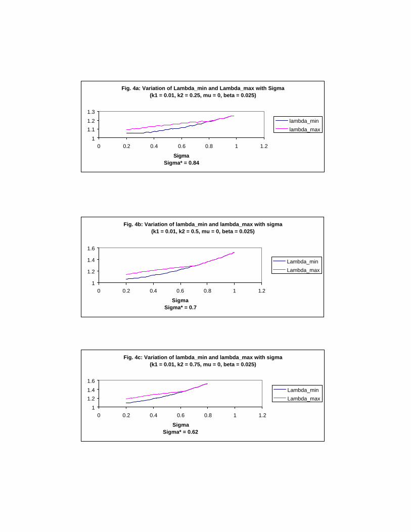
Fig. 4a: Variation of Lambda_min and Lambda_max with Sigma(k1 = 0.01, k2 = 0.25, mu = 0, beta = 0.025)

1

1.1

1.2

1.3

0 0.2 0.4 0.6 0.8 1 1.2

SigmaSigma* = 0.84

lambda_min

lambda_max

Fig. 4b: Variation of lambda_min and lambda_max with sigma(k1 = 0.01, k2 = 0.5, mu = 0, beta = 0.025)

1

1.2

1.4

1.6

0 0.2 0.4 0.6 0.8 1 1.2

SigmaSigma* = 0.7

Lambda_min

Lambda_max

Fig. 4c: Variation of lambda_min and lambda_max with sigma(k1 = 0.01, k2 = 0.75, mu = 0, beta = 0.025)

1

1.2

1.4

1.6

0 0.2 0.4 0.6 0.8 1 1.2

SigmaSigma* = 0.62

Lambda_min

Lambda_max

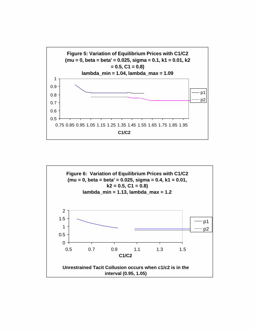
Figure 6: Variation of Equilibrium Prices with C1/C2 (mu = 0, beta = beta' = 0.025, sigma = 0.4, k1 = 0.01,

k2 = 0.5, C1 = 0.8)lambda_min = 1.13, lambda_max = 1.2

0

0.5

1

1.5

2

0.5 0.7 0.9 1.1 1.3 1.5C1/C2

Unrestrained Tacit Collusion occurs when c1/c2 is in the interval (0.95, 1.05)

p1

p2

Figure 5: Variation of Equilibrium Prices with C1/C2 (mu = 0, beta = beta' = 0.025, sigma = 0.1, k1 = 0.01, k2

= 0.5, C1 = 0.8)lambda_min = 1.04, lambda_max = 1.09

0.5

0.6

0.7

0.8

0.9

1

0.75 0.85 0.95 1.05 1.15 1.25 1.35 1.45 1.55 1.65 1.75 1.85 1.95

C1/C2

p1

p2

Strategic Relationships between Buyers and Sellers under ... · Strategic Relationships between...

Documents

Transcript of Strategic Relationships between Buyers and Sellers under ... · Strategic Relationships between...