Strategic implications of counter-geoengineering: clash or cooperation? Daniel Heyen, Joshua Horton, Juan Moreno-Cruz December 2018 Centre for Climate Change Economics and Policy Working Paper No. 345 ISSN 2515-5709 (Online) Grantham Research Institute on Climate Change and the Environment Working Paper No. 313 ISSN 2515-5717 (Online)

This working paper is intended to stimulate discussion within the research community and among users of research, and its content may have been submitted for publication in academic journals. It has been reviewed by at least one internal referee before publication. The views expressed in this paper represent those of the authors and do not necessarily represent those of the host institutions or funders.

The Centre for Climate Change Economics and Policy (CCCEP) was established by the University of Leeds and the London

School of Economics and Political Science in 2008 to advance public and private action on climate change through

innovative, rigorous research. The Centre is funded by the UK Economic and Social Research Council. Its third phase

started in October 2018 with seven projects:

1. Low-carbon, climate-resilient cities

2. Sustainable infrastructure finance

3. Low-carbon industrial strategies in challenging contexts

4. Integrating climate and development policies for ‘climate compatible development’

5. Competitiveness in the low-carbon economy

6. Incentives for behaviour change

7. Climate information for adaptation

More information about CCCEP is available at www.cccep.ac.uk

The Grantham Research Institute on Climate Change and the Environment was established by the London School of

Economics and Political Science in 2008 to bring together international expertise on economics, finance, geography, the

environment, international development and political economy to create a world-leading centre for policy-relevant

research and training. The Institute is funded by the Grantham Foundation for the Protection of the Environment and the

Global Green Growth Institute. It has six research themes:

1. Sustainable development

2. Finance, investment and insurance

3. Changing behaviours

4. Growth and innovation

5. Policy design and evaluation

6. Governance and legislation

More information about the Grantham Research Institute is available at www.lse.ac.uk/GranthamInstitute

Suggested citation:

Heyen D, Horton J and Moreno-Cruz J (2018) ‘Strategic implications of counter-geoengineering: clash or cooperation?’

Centre for Climate Change Economics and Policy Working Paper 345/Grantham Research Institute on Climate Change and

the Environment Working Paper 313. London: London School of Economics and Political Science

Strategic Implications of Counter-Geoengineering:

Clash or Cooperation? ∗

Daniel Heyen†

Chair of Integrative Risk Management and EconomicsETH Zurich

Joshua HortonJohn A. Paulson School of Engineering and Applied Sciences

Harvard University

Juan Moreno-CruzSchool of Environment, Enterprise and Development

University of Waterloo

December 10, 2018

Abstract

Solar geoengineering has received increasing attention as an option to temporar-ily stabilize global temperatures. A key concern is that heterogeneous preferencesover the optimal amount of cooling combined with low deployment costs may al-low the country with the strongest incentive for cooling, the so-called free-driver,to impose a substantial externality on the rest of the world. We analyze whetherthe threat of counter-geoengineering technologies capable of negating the climaticeffects of solar geoengineering can overcome the free-driver problem and tilt thegame in favor of international cooperation. Our game-theoretical model of countrieswith asymmetric preferences allows for a rigorous analysis of the strategic inter-action surrounding solar geoengineering and counter-geoengineering. We find thatthe free-driver outcome becomes unstable once counter-geoengineering is available,but not always with benign effects. The presence of counter-geoengineering leadsto either a climate clash where countries engage in a non-cooperative escalation ofopposing climate interventions (negative welfare effect), a moratorium treaty wherecountries commit to abstain from either type of climate intervention (indeterminatewelfare effect), or cooperative deployment of solar geoengineering (positive welfareeffect). We show that the outcome depends crucially on the degree of asymmetry intemperature preferences between countries.

∗We gratefully acknowledge funding from the ESRC Centre for Climate Change Economics and Policyand Grantham Foundation for the Protection of the Environment and thank the organisers of the HarvardSolar Geoengineering Research Residency. D.Heyen gratefully acknowledges support from the GermanResearch Foundation (DFG), grant HE 7551/1. Moreno-Cruz acknowledges support from the CanadaResearch Chairs program. This paper has benefited substantially from discussions and comments at thefollowing events: seminars at FEEM Milan and the Institute for Science, Innovation and TechnologyOxford; the EAERE 2017 conference in Athens, Climate Engineering Conference CEC 17 in Berlin,EENR 2018 workshop in Orleans, WCERE 2018 conference in Gothenburg and the GRI workshop atLSE.†Corresponding author. dheyen@ethz.ch

1

Keywords: climate intervention; solar geoengineering; counter-geoengineering; free-driver; strategic conflicts; game theory; cooperation; externality; global warming;international environmental agreementsJEL Codes: Q54; H41; D62; D02; D74.

2

Strategic Implications of Counter-Geoengineering:

Clash or Cooperation?

December 10, 2018

Abstract

Solar geoengineering has received increasing attention as an option to temporar-ily stabilize global temperatures. A key concern is that heterogeneous preferencesover the optimal amount of cooling combined with low deployment costs may al-low the country with the strongest incentive for cooling, the so-called free-driver,to impose a substantial externality on the rest of the world. We analyze whetherthe threat of counter-geoengineering technologies capable of negating the climaticeffects of solar geoengineering can overcome the free-driver problem and tilt thegame in favor of international cooperation. Our game-theoretical model of countrieswith asymmetric preferences allows for a rigorous analysis of the strategic inter-action surrounding solar geoengineering and counter-geoengineering. We find thatthe free-driver outcome becomes unstable once counter-geoengineering is available,but not always with benign effects. The presence of counter-geoengineering leadsto either a climate clash where countries engage in a non-cooperative escalation ofopposing climate interventions (negative welfare effect), a moratorium treaty wherecountries commit to abstain from either type of climate intervention (indeterminatewelfare effect), or cooperative deployment of solar geoengineering (positive welfareeffect). We show that the outcome depends crucially on the degree of asymmetry intemperature preferences between countries.

Keywords: climate intervention; solar geoengineering; counter-geoengineering; free-driver; strategic conflicts; game theory; cooperation; externality; global warming;international environmental agreementsJEL Codes: Q54; H41; D62; D02; D74.

1 Introduction

One option for addressing climate change that is gaining increased attention is Solar

Geoengineering (SG), also known as Solar Radiation Management (SRM) (National

Research Council 2015). SG aims at (partially) compensating the global warming caused

by increased atmospheric levels of greenhouse gases by either releasing cooling particles in

the stratosphere (stratospheric aerosol injection) or modifying marine cloud reflectivity

(marine cloud brightening). While an optimally designed and implemented SG scheme

appears to have the potential to reduce global temperature damages (Moreno-Cruz et al.

2012; Keith and MacMartin 2015; National Research Council 2015), there are concerns

that SG’s potential benefits are reduced and possibly even reversed in a decentralized

world of international ’anarchy’. A key fear is that presumably low deployment costs

1

(McClellan et al. 2012; Smith and Wagner 2018) together with asymmetric preferences

over the optimal global temperature change (Heyen et al. 2015) may result in unilateral

SG deployment that harms the rest of the world (Horton 2011; National Research Council

2015; Pasztor et al. 2017). This has been termed the “free-driver” problem (Weitzman

2015).1

Against this backdrop of potentially welfare deteriorating strategic incentives sur-

rounding a potentially beneficial technology, a recent paper (Parker et al. 2018) explores

the idea of counter-geoengineering (CG), or a set of technologies that would give coun-

tries threatened by or subject to the free-driver’s whims a tool for quickly negating what

they regard as harmful SG. While states opposed to unilateral SG could impose a variety

of indirect costs (such as trade sanctions) on a free-driver in an effort to halt deploy-

ment (Horton 2011), CG would entail a direct response intended to curb such behavior.

In principle, CG could be either ’neutralizing’ (e.g. injecting a base to counteract the

sulphate aerosols most commonly considered for SG) or ’countervailing’ (e.g. the release

of a warming agent such as difluoromethane to reverse the effects of SG particles). The

reason why the availability of such CG capabilities might prove beneficial is obviously

not because further global warming is globally desirable; rather, the very availability

of CG might deter the free-driver from unilateral SG deployment and instead promote

international cooperation on climate interventions. If CG has this potential to steer

climate technology use to overall beneficial levels, then there is a case for countries to

invest in CG today as a deterrent to future unilateral SG use.

The present paper provides a first rigorous analysis of the strategic effects of intro-

ducing SG and CG into an otherwise standard model of climate economics. We regard

SG and CG as two separate and contrasting forms of climate intervention. With this

understanding, we model climate intervention (via either SG or CG) as a public good

game: the operational costs of any climate intervention are borne only by the deploy-

ing country, whereas the resulting global temperature change affects all countries. The

latter is captured by a non-monotonic benefit function that exhibits an optimal level

of global temperature change. A key assumption in our model is that countries dis-

agree about the optimal temperature change and therefore their preferred amount of

climate intervention. We give countries two distinct options for cooperation. The first

is a deployment treaty where countries jointly decide on the climate intervention that

maximizes the coalition’s overall payoff. The second option, which constitutes one of

the novel contributions of the present paper, is a moratorium treaty. In a moratorium,

an idea often raised in the geoengineering debate (Parker 2014; Victor 2008; Zurn and

1The ’free-driver’ terminology emphasizes two things: first, the public good nature of interventionsin the global climate, i.e. non-excludability and non-rivalry; and second, the potential for a single actorto get in the ’driver seat’ (due to low deployment costs) and shape the global climate as she wishes, incontrast to the well-known ’free-rider’ problem (Stavins 2011). To emphasize heterogeneous preferences,Weitzman (2015) also refers to SG as a ’public gob’, that is, a public good or bad, depending on theamount deployed.

2

Schafer 2013; Parson and Keith 2013), countries commit themselves to abstain from any

form of climate intervention. As usual, we assume each country individually determines

its willingness to cooperate by comparing payoffs under alternative treaties to the non-

cooperative outcome. We study how CG affects the incentives to cooperate by analyzing

the game first when only SG is available and hence climate intervention is restricted to

cooling; and second when CG is also available and countries are able to cool or warm.

Despite this parsimonious setting, our model delivers a rich set of findings. In the

absence of CG, if countries are sufficiently different in their preferred temperature, the

non-cooperative outcome is a free-driver equilibrium. If countries have similar preferred

temperatures, then the non-cooperative outcome is a free-rider equilibrium. In both

cases, cooperation incentives are overall weak: The moratorium treaty is never supported

by both countries and therefore unstable, and the deployment treaty is only stable for

a relatively small set of parameter constellations. The effect of introducing CG is to

render the free-driver equilibrium unstable: those who regard the free-driver’s cooling as

excessive now have a tool to counteract it, and they use it. Absent the opportunity to

cooperate, this results in a ’climate clash’, an escalation of cooling by SG and warming

by CG that typically has no winners and is overall sharply detrimental. If cooperation is

an option, however, this bleak outlook of CG in a non-cooperative world may encourage

countries to work together. In particular, the free-driver, typically unwilling to cooperate

in the absence of CG, may be ready to compromise on the amount of climate intervention.

Yet cooperation is not assured, and the outcome might still be a destructive climate clash.

And even if cooperation does occur, it might take the form of a moratorium, which

could be worse than the free-driver outcome if climate damages are sufficiently high.

The outcome depends crucially on the degree of asymmetry in temperature preferences

between countries.

Our paper contributes to two strands of the literature. The first is the emerging liter-

ature on strategic interaction and governance surrounding solar geoengineering (Klepper

and Rickels 2014; Horton 2011; Barrett et al. 2014; Barrett 2014). We make three specific

contributions to this literature. The first pertains to research on non-cooperative geo-

engineering outcomes under different types of asymmetry (Moreno-Cruz 2015; Manoussi

and Xepapadeas 2017; Manoussi et al. 2018; Urpelainen 2012; Weitzman 2015; Heyen

2016). These papers, with the exception of Weitzman (2015) and Heyen (2016), focus on

asymmetry in terms of heterogeneous side-effects or different levels of uncertainty but

maintain the assumption that countries’ preferences regarding the desired climate out-

come are perfectly aligned. Our work advances this literature by putting heterogeneous

preferences over the global average temperature center-stage. We believe that this source

of asymmetry is crucial to capture the idea of excessive SG, frequently referred to as

’free-driving’.2 Second, we extend Weitzman (2015) and Heyen (2016) in several ways,

2Emmerling and Tavoni (2017) interpret free-driving as over-provision relative to the cooperative(global first-best) solution. This is why free-driving in their sense can also occur in settings with sym-

3

most importantly by adding the option of CG. The first paper that has put CG center-

stage is Parker et al. (2018). We advance their analysis by using a richer and calibrated

game-theoretical model (also see Appendix C on the timing of the non-cooperative game)

and by studying incentives for cooperation. Third, cooperation incentives surrounding

SG have been studied by Millard-Ball (2012) and Ricke et al. (2013). We extend this

literature in two ways: first, we study heterogeneous preferences over the global tem-

perature and show that cooperation incentives crucially depend on the degree to which

countries disagree about the desired climate. Second, we introduce CG and demonstrate

that CG significantly alters countries’ incentives to cooperate.

The second strand of the literature we contribute to is the environmental economics

literature on public goods, externalities and cooperation, see for instance Barrett (1994)

and Finus (2008). Despite the dominant approach of considering symmetric players,

the subtle and important role of heterogeneity in strategic environmental settings has

been noted and emphasized (Barrett 2001; McGinty 2007; Finus and McGinty 2018).

In this context our paper makes three innovations. First, following Weitzman (2015)

and Heyen (2016) we allow for the over-provision of a public good by modelling non-

monotonic benefit functions with heterogeneous optimal levels, a feature not present

in other asymmetric public good settings; in contrast to Weitzman (2015), however,

we include deployment costs, which gives rise to much richer findings, and situate this

discussion in a standard public-good setting with a smooth benefit function. The second

innovation of our paper is to consider CG, which essentially allows agents to make

‘negative’ contributions to a public good, an aspect that may be of more general interest

in future research beyond geoengineering. Finally, the third contribution of our paper to

the environmental economics literature on public goods and cooperation is to introduce a

moratorium treaty, i.e. we give agents the option to jointly abstain from contributions to

the public good altogether. This form of cooperation, which has not received attention

in the literature – unsurprising in light of the focus on symmetric settings – may be

of general interest for the analysis of strategic interaction of agents with asymmetric

preferences, in particular when side-payments are not available.

We proceed as follows. Sec. 2 presents the model components in detail, with a focus

on the case of two countries. Sec. 3 analyzes the deployment stage, in particular the

non-cooperative outcomes both with and without CG; these non-cooperative outcomes

are the reference points for countries when choosing whether to cooperate, discussed

in Sec. 4. Sec. 5 calibrates the model. We then present two robustness checks: Sec.

6 relaxes the assumption that SG and CG have the same cost structure and Sec. 7

generalizes from two to n countries. Sec. 8 concludes.

metric preferences because countries do not account for the externalities caused by SG.

4

2 The Model

In our model two countries with asymmetric preferences decide on climate intervention

levels, i.e. changes to global temperatures using either SG or CG. Initially we assume

SG and CG are symmetric in terms of costs, but we relax that assumption in section 6.

The general case with n countries is covered in section 7. Because changes to global tem-

peratures affect every country, we model climate intervention as a public good provision

game.

2.1 Timing of Events

Figure 1 gives a graphical representation of the two stages of the game. In the first

stage the two countries can cooperate by forming a climate intervention treaty. The two

available options are a moratorium treaty, in which the countries commit themselves to

deploy neither SG nor CG, and a deployment treaty, in which the countries within the

coalition commit themselves to choose technology levels so as to maximize the coalition’s

sum of payoffs. By definition, the deployment treaty implements the climate intervention

that maximizes global welfare. If neither treaty comes into effect, countries in the second

period choose their climate intervention levels simultaneously and non-cooperatively.3 In

order to assess the game-changing potential of CG we contrast two cases. First, the ‘SG

only’ case when CG is not available and hence climate interventions are restricted to

cooling. We then compare this with the ‘CG available’ case in which countries have the

option to increase or decrease global mean temperatures. The non-cooperative outcome

depends on whether CG is available or not, and this will in turn have implications for

the attractiveness of the treaties.

2.2 Definitions and Assumptions

Climate intervention levels gi ∈ R, i = A,B, are measured in terms of the resulting

temperature change. The global average temperature under climate change T0 – the

status quo temperature countries face when making their climate intervention choice –

is normalized to zero, T0 = 0.4 Hence, the change in global average temperature T due

to climate intervention is

T = gA + gB. (1)

We assume that costs and benefits are quadratic (Barrett 1994; McGinty 2007; Finus

3We consider the simultaneous game structure to be the most realistic representation of non-cooperative interaction on climate intervention and therefore deviate from the sequential order in Parkeret al. (2018). A detailed discussion of the time structure of our model can be found in Appendix C.

4This temperature includes the effects of any previous mitigation efforts. We do not model mitigationexplicitly. The reason is that we are interested in the strategic interaction surrounding SG and CGthat can be expected to unfold on a fairly short timescale: climate interventions would have an almostimmediate temperature response effect, whereas the effects of mitigation need much longer to materialize.

5

1. TREATY 2. DEPLOYMENT

A

B + −

+ −

Moratorium Treaty

Deployment Treaty

A B

A

B + −

+ −

A B

A

B + −

+ −

A

B + −

+ −

CG available

SG only

Non-cooperative

Figure 1: Timing of the game, illustrated for two countries labelled A and B. In the first stagethe countries decide whether to cooperate via a moratorium treaty (countries commit to deployneither SG nor CG) or a deployment treaty (countries commit to implement the coalition’s op-timal climate intervention). If neither treaty comes into effect, countries choose their technologylevels (non-positive in the ‘SG only’ case, any level in the ‘CG available’ case) non-cooperatively.

and Rubbelke 2013; Diamantoudi and Sartzetakis 2006; Heyen 2016).5 The costs are

C(gi) =c

2g2i , i = A,B (2)

with c > 0.6 We assume for simplicity that SG and CG have the same country-

independent cost structure. The general case with asymmetric cost structures for SG

and CG is covered in Section 6. The climate benefits are

Bi(T ) = − b2

(Ti − T )2 , i = A,B (3)

with b > 0.7 We define the benefit-cost parameter θ = b/c. In contrast to operational

costs which are private, the benefit function B reflects the public good nature of the

climate intervention: Benefits depend on the global average temperature T and hence

5The calibration in Sec. 5 justifies this assumption.6For the analysis within a public good framework it is crucial to focus on those costs that are borne by

each country individually. In the context of a climate intervention these are the direct operational costsof modifying the global climate. Indirect costs that are climate-related are captured within the non-monotonic benefit function B. Indirect costs not related to climate indicators, e.g. health impacts fromsulfur particles, are not incorporated in our simple model; including them would likely only strengthenour results as they add another source of external effects, see the discussion in section 8. The costfunction (2) captures that the deployment costs a country has to bear are convex in that country’s levelof geoengineering deployment but is not able to capture that deployment costs may also be affected bydeployment by others.

7Here we make the simplifying assumption that countries assess climate outcomes using temperatureas a proxy for all indicators of climate change. Of course, these simplification comes with limitationsand in section 8 we discuss the role of indicators other than temperature.

6

on the climate intervention levels of both countries. The benefits are highest at T = Ti

which justifies calling Ti country i’s preferred temperature. For a country that suffers

from climate change, which is the typical situation, Ti < 0.

Country i’s payoff under the climate intervention profile g = (gi)i=A,B is

πi(g) = Bi(T )− C(gi) . (4)

A central component of the model is to allow for different Ti and hence heterogeneous

preferences over the optimal amount of climate intervention.8 Without loss of generality

let TA ≤ TB. Accordingly, from now on A is the country that favours relatively strong

deployment of SG, whereas country B prefers moderate cooling or no cooling at all. We

define the mean optimal temperature change T = TA+TB2 and write

TA = T −∆ , TB = T + ∆, where ∆ =TB − TA

2. (5)

We refer to ∆ as the asymmetry parameter which equals the standard deviation of the

optimal temperature changes TA and TB. For ∆ = 0, both countries agree on how much

the climate ought to change; the higher ∆, the higher the disagreement between the two

countries in terms of how to set the global thermostat.9 One of the advantages of this

definition of ∆ is that it can easily be extended to the general n country case that we

discuss in section 7.

Regarding the overall desirability of some amount of SG, we assume that at the time

countries consider a climate intervention through SG (or CG), past efforts at mitigation

and ’negative emissions’ such as bioenergy with carbon capture and storage (BECCS)

have proved insufficient to curb temperatures.

Assumption 1. The world without any climate intervention is on average too warm,

T < 0.

In particular, TA < 0. We do not impose assumptions on TB, so country B might

prefer a warmer climate, TB > 0.

8It is worth emphasizing that our model’s approach to capture heterogeneity in terms of differentoptimal levels of a public good is novel. With the exception of Weitzman (2015) and Heyen (2016), thetypical focus in the literature has been to assume the same optimal level of the public good but differentslopes of the marginal benefit function (e.g. McGinty 2007).

9A simple illustrative example provides evidence that countries may prefer different global averagetemperatures. Assume country A and country B to have pre-industrial temperatures of 16◦C and 10◦C,respectively. Further assume that climate change increases temperatures in both countries by 3◦C. Theclimate impact literature suggests that growth rates are maximal for a certain universal, i.e. country-independent, temperature; Burke et al. (2015) find growth rates to follow a quadratic inverted U shapewith a maximum at around 13◦C. If country A and country B both regard 13◦C as their optimaltemperature, then we have in our notation TA = −6◦C and TB = 0◦C, resulting in ∆ = 3◦C. Such auniversal optimal temperature, even if countries’ preferences are only partially determined by it, providesa strong argument for heterogeneous preferences over climate intervention in a world of heterogeneousbaseline temperatures.

7

2.3 The Decision to Enter a Treaty

We model a climate intervention treaty in line with the literature on international envi-

ronmental agreements (e.g. Barrett 1994, 2001; Finus 2008). Instead of joint decisions

on emission abatement levels, countries in a coalition here jointly decide on climate in-

tervention levels. In the first type of treaty, the deployment treaty, countries choose

the amount of SG that maximizes the coalition’s total payoff, i.e. the sum of payoffs

across its members. One of the innovations of our paper is to allow for a second type

of treaty, the moratorium treaty. Here, the countries commit themselves to abstain

from climate interventions altogether, gi = 0. One reason to consider this additional

type of treaty is the importance of a moratorium in the geoengineering debate (Victor

2008; Parker 2014); furthermore, the aspect of winners and losers is particularly pro-

nounced in the present paper and a moratorium treaty – by definition less appealing

than a deployment treaty in terms of the sum of payoffs – might possibly be attractive

due to its distributional implications.

In this context it is important to note that we do not include side payments (also

known as transfers) in our model. The importance of side payments in increasing the at-

tractiveness of cooperation has often been noted, especially for countries with asymmet-

ric preferences (McGinty 2007; Barrett 2001).10 Yet we often observe that international

treaties designed to overcome domestic interests face strong opposition and that side

payments in particular are often seen as politically unacceptable (Gampfer et al. 2014;

Diederich and Goeschl 2017). This suggests that studying incentives for cooperation

that do not rely on transfers is an important benchmark. The deployment treaty and

moratorium treaty are two specific, yet salient, forms of cooperation in the absence of

transfers.

We model a country’s choice regarding treaty participation as the submission of a

ranked ordering of the country’s preference over the three possible outcomes, i.e. the

non-cooperative outcome, the deployment treaty and the moratorium treaty. Stability

of a treaty is defined relative to the non-cooperative outcome. With only two countries,

the condition for a coalition to be stable reduces to internal stability, i.e. whether both

countries want to be a member of the coalition compared to the non-cooperative Nash

solution. Furthermore, with only two countries it does not make a difference whether

the coalition is modelled as an open membership game, in which a country can enter a

coalition without the other members’ invitation, or an exclusive club, where access to a

coalition is conditional on the members’ consent Ricke et al. (2013). See section 7 for a

treatment of the case with n countries. Note that coalitions that are stable in the ‘SG

only’ scenario need not be stable under the ‘CG available’ case, and vice versa.

As we will show below, the deployment and moratorium treaty can both be stable at

10Indeed, in the absence of negotiation and transaction costs, it is well known that transfer schemesexist to ensure that the socially optimal configuration makes each party better off (Coase 1960).

8

the same time. While equilibrium selection is not a focus of our paper, we aim to make

the analysis in the n = 2 case as easy to follow as possible and hence make the following

tie-breaking assumption.

Assumption 2 (Tie-breaking rule). If both treaties are stable, i.e. if both countries are

willing to enter either of the two treaties, then the one most preferred by both countries

comes into effect if there is such a clear ordering; if countries disagree on the preferred

order, we assume that the moratorium treaty comes into effect.

The rationale for this tie-breaking rule is that the status quo of non-deployment may

be a focal point, for instance because an error of geoengineering ’commission’ is assumed

to be worse than an error of geoengineering ’omission’ (Weitzman 2015). We will see

below that equilibrium selection has a significant impact on the analysis.

We proceed with the equilibrium analysis. We first discuss the non-cooperative

equilibria, the fallback option when none of the treaties comes into effect. The relative

attractiveness of the non-cooperative case, in turn, determines countries’ willingness to

enter the moratorium and/or deployment treaty.

3 Optimal Deployment and Non-cooperative Equilibria

We solve the equilibrium via backward induction and thus begin our description with

the climate intervention deployment stage. The countries simultaneously choose gi ∈ R,

i = A,B. In the ‘SG only’ case, deployment is restricted to cooling, gi ≤ 0. When CG

is available, any temperature level gi ∈ R is feasible.11

3.1 Global Optimum

We denote by (g∗∗i )i=A,B the socially optimal configuration that maximizes global welfare

π(g) = πA(g) + πB(g). The solution to this problem following standard procedure is

g∗∗i =2θ

4θ + 1T , i = A,B . (6)

It is efficient that both countries deploy the same amount of solar geoengineering due to

the homogeneous cost structure. Owing to T < 0 (Assumption 1), the socially optimal

deployment scheme features SG deployment by both countries. Whether CG is available

or not has, therefore, no implications for the socially optimal deployment profile. It is

straightforward to see that (6) increases in the benefit-cost ratio θ.

11The absence of an upper limit on the level of CG corresponds to ’countervailing’ CG (Parker et al.2018), e.g. the release of a potent GHG. The maximal amount of ’neutralizing’ CG, in contrast, would bea function of the deployed SG level. We find that CG levels are smaller than SG levels, see below, so thatin the context of the present paper it is inconsequential whether we understand CG as countervailing orneutralizing.

9

3.2 Non-cooperative equilibria

The first step in determining the non-cooperative Nash equilibria is to calculate the

best response functions. The conceptually simplest case is when CG is available and

hence gi ∈ R unrestricted. In this case, the best response of country i to the other

country’s climate intervention level g−i is characterized by the first-order condition

dπi(gi; g−i)/dgi = 0. In the ‘SG only’ case, we also need to check whether the non-

positive constraint binds. We get the best response function

gi(g−i) =

min{

θθ+1 (Ti − g−i) , 0

}SG only

θθ+1 (Ti − g−i) CG available

(7)

Figure 2 shows how the best response functions depend on the asymmetry ∆.

gB

-4 -3 -2 -1 0 1 2

g A

-4

-3

-2

-1

0

1

2

gA

(gB

)

gB

(gA

)

(a) ∆ = 0 ◦C

gB

-4 -3 -2 -1 0 1 2

g A

-4

-3

-2

-1

0

1

2

gA

(gB

)

gB

(gA

)

(b) ∆ = 0.4 ◦C

gB

-4 -3 -2 -1 0 1 2

g A

-4

-3

-2

-1

0

1

2

gA

(gB

)

gB

(gA

)

(c) ∆ = 0.8 ◦C

gB

-4 -3 -2 -1 0 1 2g A

-4

-3

-2

-1

0

1

2

gA

(gB

)

gB

(gA

)

(d) ∆ = 1.2 ◦C

Figure 2: Best response functions (country A in red, country B in blue) for different asymmetrylevels ∆. In all plots θ = 2 and T = −2 ◦C. The solid lines and dashed lines show the bestresponse functions without CG and with CG, respectively. The unfilled circle indicates thesocially optimal benchmark (g∗∗A , g

∗∗B ). The asymmetry threshold is ∆ = 0.4 ◦C, see (8). For

∆ > ∆ the equilibrium outcome, indicated by a filled black circle, depends on whether CG isavailable or not.

We now summarize non-cooperative equilibria in the ‘SG only’ and ‘CG available’

scenarios and hence determine the game-changing effect of CG in the absence of coop-

eration possibilities. We define the asymmetry threshold

∆ := − 1

2θ + 1T . (8)

The asymmetry threshold plays an important role in the following discussion, as it helps

explain which equilibria obtain under different conditions.

Proposition 1 (Game-changing potential of CG. Non-cooperative equilibria). There is

a unique Nash equilibrium and the outcome depends on parameter settings and whether

CG is available:

(i) The ‘SG only’ case. For low levels of asymmetry, ∆ < ∆, both countries engage

10

in SG. We refer to this outcome as the free-rider equilibrium,

g∗A =θ

2θ + 1T − θ∆ < 0 , g∗B =

θ

2θ + 1T + θ∆ < 0 . (9)

For high levels of asymmetry, ∆ ≥ ∆, only country A deploys SG. We refer to this

outcome as the free-driver equilibrium,

g∗A =θ

θ + 1TA , g∗B = 0 . (10)

(ii) The ‘CG available’ case. For low levels of asymmetry, ∆ < ∆, there is no incentive

to deploy CG. The unique equilibrium is therefore the free-rider outcome (9).

For high levels of asymmetry, ∆ ≥ ∆, country A cools and, simultanouesly, country

B warms. We refer to this outcome as the climate clash equilibrium,

g∗A =θ

2θ + 1T − θ∆ < 0 , g∗B =

θ

2θ + 1T + θ∆ ≥ 0 . (11)

(iii) The transformation from free-driver to climate clash is always detrimental for

country A and detrimental for country B iff θ > 1+√

52 . The transformation is

unambiguously detrimental in terms of overall welfare.

Proof. See appendix A.

Figure 3 shows climate intervention levels for both countries under the non-cooperative

equilibria as a function of the asymmetry level ∆. For comparison we include the total

SG level under the moratorium treaty (i.e. zero) and the deployment treaty. The free-

driver SG level (solid purple line) depends on country A’s optimal temperature change

TA but not on TB and hence the cooling intensifies as the asymmetry level ∆ increases.

The total temperature change in the climate clash (solid red line) matches the free-rider

level (solid orange line) and is independent of the asymmetry level ∆, but is the result

of ever diverging SG and CG levels (dashed and dot-dashed red lines) by country A and

country B respectively.12

The free-rider equilibrium is a well-known outcome in the literature; in particular,

the symmetric case ∆ = 0 is of this type. The more interesting outcome in the ‘SG

only’ case is the free-driver equilibrium. The terminology is from Weitzman (2015) who

develops the concept of over-provision of a public good in a setting without deployment

costs and with a specific kinked utility function. Our definition coincides with the one in

Heyen (2016). The defining characteristic of the free-driver equilibrium is that cooling is

excessive from country B’s perspective, T ≤ TB, and country A is essentially in control

of the global thermostat. This excessive cooling does not necessarily imply that country

12The total deployment level in the climate clash is independent of the level of asymmetry if and onlyif SG and CG have the same cost structure, see section 6.

11

Asymmetry "0 0.5 1 1.5 2 2.5 3

Clim

ate

inte

rven

tion

(°C

)

-3

-2

-1

0

1Moratorium TreatyDeployment TreatyFree RiderFree DriverClimate Clash

Figure 3: Climate intervention levels of the non-cooperative equilibria as a function of the asym-metry ∆. The parameter settings are as in Figure 2, i.e. θ = 2 and T = −2 ◦C. The vertical lineis at the asymmetry threshold ∆. The dashed and dot-dashed lines represent the deploymentby country A and country B, respectively, while the solid lines show net levels. For compari-son we include the total climate intervention levels under the moratorium treaty (zero) and thedeployment treaty (the total level is twice the amount in (6)).

B is worse off relative to a world without any climate intervention. Importantly for our

analysis, the free-driver equilibrium becomes unstable once CG is available. Country B

now has a tool to counter the over-provision of the public good, and due to zero marginal

costs (at the point of non-deployment), country B uses this tool. The best response of

country A, in turn, is to increase its SG efforts. The only reason why SG and CG levels

are bounded in this escalation equilibrium is the convexity of the cost function.

This section has demonstrated that CG renders the free-rider equilibrium unstable,

replacing it with a climate clash. This game-changing effect is overall detrimental as

countries waste significant resources on SG and CG. But can CG play a more positive

role in the context of cooperation? The next section is dedicated to this question.

4 Incentives for Cooperation

This section analyzes the incentives to cooperate on climate intervention via either a

deployment treaty or a moratorium treaty. We begin with the ‘SG only’ case in section

4.1 and cover the ‘CG available’ case in section 4.2. All findings are illustrated in Figure

4.

12

4.1 Cooperation incentives when only SG is available

The non-cooperative deployment equilibria derived in the previous section (cf. Propo-

sition 1) are the appropriate reference points when countries are deciding whether they

are willing to cooperate by entering a moratorium or deployment treaty. We start with

the low asymmetry case where non-cooperation would result in the free-rider outcome.

Proposition 2 (Cooperation incentives in the ‘SG only’ case. Low asymmetry, ∆ < ∆).

Country A prefers the deployment treaty over the free-rider equilibrium irrespective of

the level of asymmetry ∆. Country B however prefers the deployment treaty only when

0 ≤ ∆ < ∆FreeRiderMax , which is therefore the region where the deployment treaty comes into

effect. Both countries prefer the non-cooperative free-rider to the moratorium treaty.

Proof. The algebraic expression for ∆FreeRiderMax ≤ ∆ and derivations are in Appendix

A.

That neither country finds the moratorium treaty attractive is intuitive as both

countries engage in SG in the non-cooperative equilibrium, indicating that they find SG

valuable even under these non-cooperative conditions; to completely abstain from SG

in a moratorium treaty then must be unattractive. The reason why country A prefers

the deployment treaty to the non-cooperative free-rider outcome is cost-sharing. The

disadvantage from having to compromise with country B on SG deployment levels is,

due to the relatively aligned preferences in low asymmetry settings, small compared to

the gain from splitting deployment costs. Country B opposes the deployment treaty

for asymmetry levels above ∆FreeRiderMax since the final temperature outcome in the non-

cooperative free-rider equilibrium is close to country B’s optimal level TB (matching this

level exactly at ∆ = ∆) and country A shoulders the main part of deployment cost. In

other words, country B is free-riding on country A’s SG deployment. We will see below

that country B’s opposition to the deployment treaty also extends into the free-driver

and climate clash region.

We move on to the case of high asymmetry, where the non-cooperative outcome

would be the free-driver equilibrium.

Proposition 3 (Cooperation incentives in the ‘SG only’ case. High asymmetry, ∆ ≥ ∆).

(i) Country A prefers the free-driver equilibrium to the moratorium treaty throughout

and prefers the deployment treaty over the free-driver equilibrium if ∆ < ∆SGMax.

(ii) Country B opts for the moratorium treaty when ∆ > ∆SGMorat and prefers the deploy-

ment treaty over the free-driver equilibrium if ∆ > ∆SGMin. It is ∆ < ∆SG

Min < ∆SGMax.

Therefore, the deployment treaty is stable for ∆SGMin < ∆ < ∆SG

Max, whereas the morato-

rium is never stable.

13

Proof. The algebraic expressions for all relevant levels of the asymmetry parameter ∆

and other derivations are in Appendix A.

Here we see for the first time the appeal of a world without any climate intervention.

Country B is willing to enter the moratorium treaty if the disadvantage from being dom-

inated by the free-driver is sufficiently high. However, it is intuitive that the moratorium

is not appealing to country A, the free-driver. Therefore, there are no circumstances un-

der which the moratorium treaty can be expected to materialize. The deployment treaty

has better chances to form. If the asymmetry exceeds ∆SGMin, the free-driver outcome is

too harmful for country B which is hence willing to enter the deployment treaty.13 Coun-

try A is also willing to enter the deployment treaty, yet under almost inverse conditions.

Specifically, for relatively moderate asymmetry levels, ∆ < ∆SGMax, the sharing of deploy-

ment costs is attractive enough to justify the compromise in temperature levels. For

asymmetry levels higher than ∆SGMax, however, the gap between the temperature com-

promise implicit in the deployment treaty and what country A would like to implement

is too wide. But ∆SGMin < ∆SG

Max, and so there do exist constellations where countries,

faced with a looming free-driver outcome, decide to cooperate.

4.2 Cooperation incentives with CG

If asymmetry is low, ∆ ≤ ∆, cooperation incentives are not changed by the availability

of CG as countries have no incentives to deploy CG anyway. We hence focus on the

high-asymmetry case where non-cooperation would result in the climate clash.

Proposition 4 (Cooperation incentives in the ‘CG available’ case. High asymmetry,

∆ ≥ ∆).

(i) Country A unambiguously prefers the deployment treaty over both the climate clash

and the moratorium treaty, and prefers the moratorium over the climate clash iff

∆ > ∆CG,AMorat.

(ii) Country B prefers the deployment treaty over the climate clash iff ∆ > ∆CGMin > ∆,

prefers the moratorium over the climate clash iff ∆ > ∆CG,BMorat, and prefers the mora-

torium over the deployment treaty iff ∆ > ∆BMorat,Treaty. While ∆CG,B

Morat < ∆CG,AMorat,

the size of ∆BMorat,Treaty relative to other critical levels depends on parameter set-

tings.

Therefore, the deployment treaty is stable for ∆ > ∆CGMin and the moratorium treaty is

stable for ∆ > ∆CG,AMorat. Under the tie-breaking Assumption 2, the separating level between

deployment treaty and moratorium treaty is ∆CGMax := max(∆CG,A

Morat,∆BMorat,Treaty).

13The intuition why country B still prefers the free-driver outcome over the deployment treaty formoderate asymmetry levels, ∆ < ∆SG

Min, is the same as in Proposition 2. The free-driver equilibriuminvolves no deployment costs for country B, and final temperature changes T , while excessive, are stillrelatively close to its optimal level TB .

14

Climate Clash

Free Rider

Deploym.Treaty

Free Driver

A B B

SG o

nly

C

G a

vaila

ble

Free Rider

Deploym.Treaty

A B A B A

A B A B

Deployment Treaty

Free Driver

A B B A

A B A B

Moratorium Treaty

Deployment Treaty

A A

B B

A A

B B

Deployment Treaty

Moratorium Treaty

A B A B

A A

B B

A B A B

Moratorium Treaty

Deployment Treaty

Non-cooperative Free Driver Free Rider

Non-cooperative Climate Clash Free Rider

Figure 4: Schematic representation of all equilibria as a function of the asymmetry parameter ∆.The upper part shows equilibria in the ‘SG only’ case, the lower part in the ‘CG available’ case.The boxes below the equilibrium labels indicate whether countries A and B are willing to joineither of the two treaties (dark fill) or not (light fill), respectively. A hatched fill indicates that acountry’s decision whether to join or not is parameter-dependent but inconsequential for the finaloutcome. When both treaties are stable (i.e. both treaties are attractive for both countries) andcountries disagree about which of the two they prefer, then our tie-breaking rule in Assumption2 resolves the disagreement. Note that the relative size of the treaty equilibria with and withoutCG depends on parameter values. See section 5 for a calibration and sensitivity analysis.

Proof. See appendix A.

The moratorium treaty is stable, i.e. preferred by both countries over the climate

clash, once the asymmetry exceeds ∆CG,AMorat. The interest in the moratorium underlines

how unattractive the climate clash is. Country B is more interested in the moratorium

treaty than country A, which is expressed both by a wider opt-in region (∆CG,BMorat <

∆CG,AMorat) and by a preference for the moratorium over the deployment treaty for levels

beyond ∆BMorat,Treaty (a preference that country A never has). This is intuitive when

we recall that temperatures under climate change absent any climate intervention (the

outcome under the moratorium treaty) are relatively less harmful for country B than

for country A. There is a simple intuition why country A is keen to cooperate via the

deployment treaty. Not only are deployment costs in the cooperative solution much lower

than in the climate clash, the social optimal SG deployment level is also more ambitious

and thus closer to TA. That country B prefers the deployment treaty to the climate clash

for moderate asymmetry levels ∆ is similar to before: country B’s deployment costs are

low and the final temperature change is relatively close to B’s optimum TB.

To summarize, we find a rich set of potential outcomes that are depicted in Figure

4. Every outcome (the non-cooperatives as well as the two treaties) materializes under

certain conditions, and the boundaries that separate different outcomes are non-trivial.

15

A parameter calibration and sensitivity analysis of the equilibrium boundaries are pre-

sented in Section 5. Our findings suggest a substantial potential of CG to change the

statics of the global thermostat game: The basic mechanism is to transform a free-driver

equilibrium into a climate clash under non-cooperative conditions, and this transforma-

tion is always bad for the free-driver A (and often for country B as well). It is this

mechanism that brings the free-driver to the negotiating table when cooperation is pos-

sible: the free-driver is now always willing to enter the global optimal deployment treaty.

In order to prevent the wasteful climate clash, the free-driver is, under certain condi-

tions, even willing to accept the otherwise very unattractive conditions of a moratorium

treaty. We will show in section 7 that this basic mechanism also shapes the general n

country case.

4.3 Welfare ranking of outcomes

We have now gained a comprehensive understanding of CG’s potential to change the

global thermostat game. Are the changes induced by CG for the better or worse? We

have partially answered this question above. Proposition 1 shows that the transformation

from a free-driver outcome to a climate clash is detrimental as it decreases global welfare.

On the other hand, whenever this bleak outlook induces countries to form a deployment

treaty, which by definition implements the global best, then CG’s game-changing effect

is beneficial. What remains to be understood is how the moratorium treaty ranks in

welfare terms. The following result shows that the transformation from a free-driver

outcome to a moratorium treaty, cf. Proposition 4, is only beneficial for high levels of

asymmetry. For completeness we also compare the moratorium treaty to the climate

clash. While not important for the welfare impact induced by the presence of CG, this

result sheds light on the value of having cooperation options once CG is part of the

game.

Proposition 5 (Welfare of Moratorium Treaty).

(i) Global welfare under the moratorium treaty is higher than in the free-driver equi-

librium iff ∆ > ∆WelfareMorat,Driver, where ∆Welfare

Morat,Driver > ∆

(ii) Global welfare under the moratorium treaty is higher than in the climate clash equi-

librium iff ∆ > ∆WelfareMorat,Clash, where ∆Welfare

Morat,Clash > ∆. In relative terms ∆WelfareMorat,Driver >

∆WelfareMorat,Clash.

Proof. See appendix A.

5 Calibration, sensitivity analysis, and welfare impact

In this section we first calibrate the model parameters b, c and T . We then determine

the sensitivity of equilibrium boundaries to changes in parameters. Finally, we discuss

16

the welfare effect of CG in the calibrated model.

5.1 Parameter calibration

Our calibration of the benefit parameter b rests on Burke et al. (2015) who show that the

relationship between (local) temperatures and growth rates follows a universal quadratic

relationship. The calibration of the cost parameter c is based on data on stratospheric

SG with sulfur aerosols. It combines data on operational cost per kg of load material with

the non-linear relation between sulfur load and reduction in radiative forcing. Finally,

T expresses the amount of atmospheric cooling required to achieve the global optimal

temperature at the point of climate intervention. This clearly depends on emissions

scenarios. Appendix B provides details on the calibration that results in the following

parameter values

b = 17.95 bn $/◦C2 , c = 8.35 bn $/◦C2 , T = −2.1◦C. (12)

We keep asymmetry ∆ as an open parameter for two reasons. First, this parameter

is the hardest to calibrate as it depends on regional/country-specific preferences over

climate outcomes (in contrast to T which is a measure of globally aggregated preferences).

Second, this provides us with a degree of freedom to describe a variety of interactions

between potentially very different agents.

5.2 Outcome boundaries and sensitivity

What outcome can we expect under parameters calibrated as above, and how sensi-

tive are the equilibrium boundaries in Figure 4 to parameter settings? Analysis of the

algebraic expression of the equilibrium boundaries (see appendix A) reveals that all

boundaries scale linearly with T and depend only on the benefit-cost ratio θ = b/c, not

b and c separately. The horizontal line in Figure 5 shows the equilibrium boundaries for

the best estimate of θ, b/c = 17.95/8.35, cf. (12). We check for sensitivity by scaling

the benefit-cost ratio upwards and downwards by two orders of magnitude. Figure 5a

and 5b depict the ‘SG only’ and ‘CG available’ cases, respectively. The solid black line

represents ∆, the asymmetry threshold from (8) that separates free-rider outcomes to

the left from free-driver (‘SG only’) and climate clash (‘CG available’) outcomes to the

right.

The first observation is that the asymmetry threshold ∆ is fairly small for the cal-

ibrated parameter values.14 This means that, in the absence of CG, even a small dis-

14What are large and small values of the asymmetry parameter ∆? Consider the example sketchedin footnote 9 where country A and country B have pre-industrial average temperatures of 16◦C and10◦C, respectively (this is not an extreme scenario as multiple regions experienced pre-industrial averagetemperatures beyond 20◦C). If both countries determined their preferences over climate interventionsbased solely on a universal optimal temperature, e.g. the 13◦C in Burke et al. (2015), then ∆ = 3K.If, less extreme, both countries considered the midpoint between pre-industrial and a certain universal

17

(a) SG only.

(b) CG available.

Figure 5: Sensitivity analysis of the equilibrium boundaries in the n = 2 case. The referencebenefit-cost ratio θ = b/c = 17.95/8.35, cf. (12), is represented as the horizontal line. To checksensitivity we scale θ upwards and downwards by two orders of magnitude. The solid black curvein both plots represents ∆. The dashed lines in (b) represent the deployment treaty boundariesof the ‘SG only’ case in (a).

temperature as optimal, then ∆ = 1.5K. In this sense it is justified to say that the asymmetry thresholdis typically fairly small.

18

agreement over the best use of SG will result in the free-driver outcome. Also note

that the deployment treaty is plausible only for the asymmetry range between 1 ◦C and

2 ◦C. Overall, the free-driver equilibrium is the most likely outcome in the ‘SG only’

case. We see that, under the calibrated parameter values, CG slightly reduces the set

of constellations under which the deployment treaty materializes, whereas the climate

clash is the predicted outcome only for a relatively narrow range of asymmetry values.

The moratorium treaty, according to our tie-breaking assumption 2, is the predicted

outcome for the ‘CG available’ case for higher values of the asymmetry parameter.

In terms of sensitivity to parameter changes, we have noted above that all boundaries

scale linearly with T . Thus we can focus on the effect of changes in the benefit-cost

ratio θ = b/c. Figure 5 demonstrates that all our observations from above are only

strengthened if θ gets higher, for instance if operational costs of a climate intervention

were significantly lower than current estimates. The free-driver is the typical outcome

in the ‘SG only’ case, and cooperation (through either a deployment or moratorium

treaty) in the ‘CG available’ case almost certain. The outcomes are very different if

we consider lower benefit-cost ratios, for instance because climate damages are seen as

relatively minor and/or climate interventions much more costly than currently expected.

Then, the free-rider outcome becomes much more plausible, in which case the presence

of CG would be inconsequential. Interestingly, the likelihood of cooperation (via either

deployment or moratorium treaty) decreases as θ decreases, and the climate clash for

high levels of asymmetry becomes increasingly plausible.

5.3 Calibrated welfare impacts

In this section we give a calibrated answer to the question whether the game-changing

potential of CG is beneficial or detrimental. Figure 6 shows the effect of CG on global

welfare.15 As in Figure 5, the horizontal axis shows the asymmetry between country

A and country B, whereas the vertical axis shows a range of benefit-cost ratios; the

horizontal line represents the best estimate of θ = b/c in (12).

There are two regions where CG does not change the game and hence leaves global

welfare unchanged (indicated by white coloring). First, all asymmetry levels to the left

of the asymmetry threshold ∆. Here, the non-cooperative outcome is the free-rider

equilibrium, and neither country wants to deploy CG in the first place. The second

15The plotted quantity in the contour plot is the welfare difference between the ‘CG available’ and the‘SG only’ case. This difference is, for each separate parameter setting, expressed in terms of the absolutewelfare under the social optimal outcome; if, for instance, global welfare under the deployment treatyis −10 units (recall that welfare levels are non-positive by assumption), then a value of −50% in thecontour plot means that CG reduces global welfare by 5 units. Note that this plot necessitates reducingone degree of freedom. While the equilibrium boundaries in Figure 5 depend only on the benefit-costratio θ = b/c, any welfare analysis depends on both parameters b and c separately. There are differentways to reduce one degree of freedom; here we stipulate that the welfare in the symmetric case ∆ = 0under the social optimal deployment profile (g∗∗A , g∗∗B ) is independent of the benefit-cost ratio θ. SeeAppendix D for more details.

19

region is where the deployment treaty was the outcome in the ‘SG case’ and remains the

outcome when CG is available.

Figure 6: Welfare effect of CG. For every pair of ∆ and b/c, the quantity plotted in the contourplot is the difference in welfare with and without CG, normalized by the social optimal welfare(i.e. welfare of the deployment treaty). Green and red colors indicate settings where the impactof CG is positive and negative, respectively, whereas white indicates that CG has no effect onglobal welfare.

We find two reasons why CG can be beneficial, indicated by green colors in Figure

6. First, CG can transform a free-driver into a deployment treaty, and our findings

suggest that this is likely for intermediate levels of asymmetry and relatively high benefit-

cost ratios. The second situation in which CG increases overall welfare is when an

extreme free-driver equilibrium is transformed into a moratorium treaty; in order for

the technology-free world to be globally preferable, the asymmetry level must be high

so that the free-driver outcome is very problematic.

If the asymmetry is not extreme, however, this transformation from free-driver to

moratorium is detrimental (potentially for both countries), represented here in dark red

colors. A second (as it turns out relatively rare) scenario in which CG is detrimental

is when a deployment treaty (bordered by the dashed lines) in the ‘SG only’ case is

transformed into either a climate clash or a moratorium treaty. Finally, there is a

third and important situation in which CG can reduce global welfare: If neither form of

cooperation is attractive, then CG transforms what used to be a bad free-driver outcome

into an even worse climate clash. This scenario is especially plausible for low benefit-cost

20

ratios.

Appendix D demonstrates that the country-specific effects of CG are fairly clear:

typically country A is worse off under CG, whereas country B benefits from the avail-

ability of CG. The mixed picture that we see in Figure 6 is hence the superposition of

generally contrasting country-specific effects.

6 Asymmetric costs

This section introduces the possibility that CG has a different cost structure than SG,

i.e. the cost function for climate interventions (2) is now differentiated into an SG and

CG part,16

C(gi) =

cSG

2 g2i gi ≤ 0

cCG2 g2

i gi > 0.(13)

To facilitate comparisons with the previous analysis we write

cSG = c , cCG = ξ · c (14)

with ξ > 0 as a measure of the asymmetry between SG costs and CG costs. The

higher ξ, the costlier is CG relative to SG. The symmetric cost structure studied above

is represented by ξ = 1. As above, we denote the benefit-cost ratio by θ = b/c; the

benefit-cost ratio for CG deployment is θ/ξ.

The clash equilibrium is the only one that involves CG. Therefore, all other equilibria

remain as before, both in terms of deployment and welfare. With the same methodology

used for Proposition 1 we show that the generalized climate clash equilibrium is

now given by

g∗A =θ

θ + (1 + θ)ξ·[ξT − (2θ + ξ)∆

], g∗B =

θ

θ + (1 + θ)ξ·[T + (2θ + 1)∆

]. (15)

Expression (11) is the special case of (15) when ξ = 1. As before we look at the

asymmetry level ∆ that separates the climate clash equilibrium from the free rider

equilibrium, defined by g∗B = 0. From (15) we see that this level is still ∆ = − T2θ+1

and therefore in particular not a function of ξ. The total deployment level g∗ in the

generalized climate clash equilibrium is

g∗ =θ

θ + (1 + θ)ξ·[(ξ + 1)T + (1− ξ)∆

]. (16)

The deployment levels in the generalized climate clash equilibrium show an intuitive

16This cost structure applies to both countries, i = A,B. Another extension could be to let differentcountries have different cost structures. Exploring this generalization is left for future research.

21

connection to the cost asymmetry parameter ξ. We find

dg∗Adξ

=(2θ + 1)θ2

(θξ + θ + ξ)2

(∆− ∆

)> 0 ,

dg∗Bdξ

= −(2θ + 1)θ(θ + 1)

(θξ + θ + ξ)2

(∆− ∆

)< 0. (17)

Due to ∆ ≥ ∆, the first expression is positive and the second negative. The higher the

CG cost, the less CG country B deploys; this implies that country A needs to do less

SG. We also see that the overall effect is negative,

dg∗

dξ= − θ(2θ + 1)

(θξ + θ + ξ)2

(∆− ∆

)< 0. (18)

The higher the costs of CG, the more cooling we see in the generalized climate clash

equilibrium.

We also immediately observe an intuitive relation between asymmetry ∆ and the

total temperature change in the generalized climate clash equilibrium. Looking at (16),

we see that an increase in asymmetry ∆ leads to more cooling if CG is costlier than SG,

ξ > 1 and to less cooling if CG is cheaper than SG, ξ < 1. The insensitivity of the total

deployment level g∗ that we observed in section 3.2, cf. Figure 3, occurs if and only if

CG and SG have the same cost structure, ξ = 1.

We now turn to the question how the relative cost structure between SG and CG

changes the statics of the game. The ’SG only’ case is not affected by a change in CG

cost. Figure 5a therefore still describes the set of equilibria without CG, irrespective of

ξ. What is affected by a change in relative costs are the equilibria in the presence of

CG. Figure 13 shows equilibria in the ’CG available’ case (i.e. variations of Figure 4)

together with plots that show the welfare changing effect of CG (i.e. variations of Figure

6) if CG is cheaper than SG, ξ < 1. Figure 7 shows the case when CG is more expensive

than SG, ξ > 1.

We can derive several insights form these figures. First, the climate clash materializes

under wider conditions both for very small as well as very large values of ξ; asymmetry

in costs of SG and CG favors the climate clash equilibrium. Second, the deployment

treaty has the best prospect when CG is costlier than SG and the difference is not too

extreme, say when ξ is around 5. Third, the moratorium treaty has the best prospect

when CG is cheaper than SG and the difference is not extreme, say ξ around 1/5. The

moratorium treaty disappears from the scene of possible outcomes when CG gets very

costly relative to SG. Fourth, as CG gets infinitely more costly than SG, the equilibria

map converges to the ’SG only’ shape, where the free driver equilibrium replaces the

climate clash. This makes sense: a very costly CG is similar to no CG at all. Finally,

the welfare effect is not straightforward. The simple intuition ’costly CG is similar to

no CG’ works for low theta values: the CG level deployed by country B here is very low,

the free driver accordingly does not have to adjust his level much. The welfare change

caused by CG accordingly is small, indicated by white/light red areas for low values

22

of θ in Figure 8. The intuition however is less straightforward for high values of the

benefit-cost ratio θ. While the statics of the game determining the equilibrium outcome

are still compatible with the ’costly CG is similar to no CG in the first place’ logic,

the welfare change is significant. The reason seems to be that high benefit-cost ratios θ

cause a major CG deployment and accordingly a major adjustment in the free-driver’s

behavior. But this requires additional research.

(a) ξ = 0.01 (b) ξ = 0.05 (c) ξ = 0.2 (d) ξ = 0.5

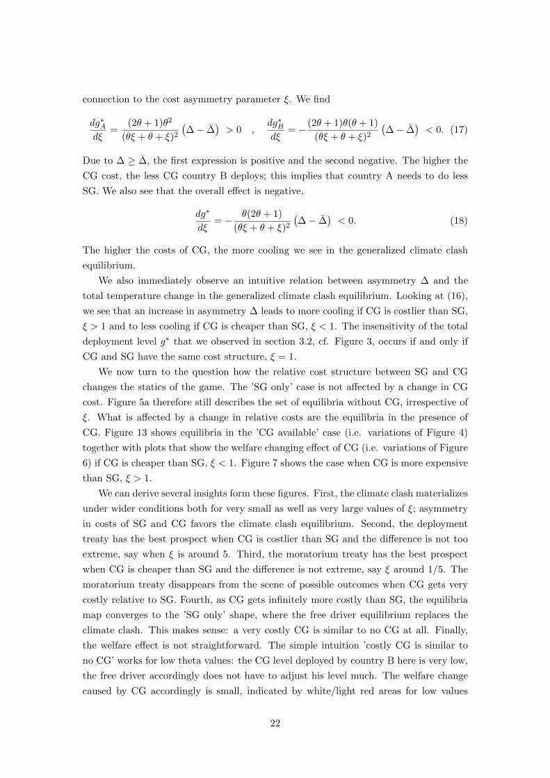
Figure 7: Asymmetric costs. CG cheaper than SG, ξ < 1.

(a) ξ = 2 (b) ξ = 5 (c) ξ = 20 (d) ξ = 100

Figure 8: Asymmetric costs. CG more expensive than SG, ξ > 1.

7 The n countries case

This section extends the setup to the general case of n countries. We derive analytical

and numerical results to check the robustness of our results derived under the two-

country model. For simplicity we go back to the assumption that SG and CG have the

same cost structure, i.e. ξ = 1 in this section.

23

7.1 Model setup

The general structure in terms of benefit function, cost function and timeline of the model

remains as before. There are now n countries, each with climate intervention level gi,

i = 1, . . . , n. The change in global average temperature T due to climate interventions

is T =∑n

i=1 gi. The mean optimal temperature change is T = 1n

∑ni=1 Ti, where Ti is

country i’s preferred global average temperature change. We keep assumption 1, i.e.

T < 0. We write

Ti = T + ∆δi , (19)

where δi ≤ . . . ≤ δn with∑n

i=1 δi = 0. We normalize 1n

∑ni=1 δ

2i = 1, so that ∆ is

the standard deviation of the optimal temperature change Ti. We call ∆ as above the

asymmetry parameter. For ∆ = 0, all countries agree on how much the climate ought to

change; increasing ∆ represents growing disagreement across countries. Note that the

definition for n = 2 in section 2 coincides with the definition given here: it is δA = −1

and δB = 1. We denote by (g∗∗i )i the socially optimal configuration that maximizes

global welfare∑n

i=1 πi(g). It is straightforward to show that

g∗∗i =nb

n2b+ cT , i = 1, . . . , n . (20)

It is efficient for all countries to deploy the same amount of SG due to the homogeneous

cost structure. Owing to T < 0 (Assumption 1), the socially optimal deployment scheme

features SG deployment by all countries. In particular, whether CG is available or not

has no implications for the socially optimal deployment profile.

7.2 Non-cooperative equilibria

As before, the asymmetry ∆ determines how many countries deploy SG in equilibrium,

and the number of countries deploying SG is monotonically decreasing in ∆. The re-

maining countries, in any case, consider the overall temperature reduction by SG as too

high and accordingly either do not deploy SG (in the ‘SG only’ case) or deploy CG (in

the ‘CG available’ case). We find a set of ∆(m) (m = 0, . . . , n) that is decreasing in

m. Here, ∆(0) = ∞ and ∆(n) = 0. We define θ = b/c, βm = mθmθ+1 and the average

optimal temperature change among the first m countries T (m) = 1m

∑mi=1 Ti. With these

preliminaries, we are ready for our next proposition.

Proposition 6 (Non-cooperative equilibria. General n). Let the asymmetry parameter

be in the interval ∆ ∈ [∆(m),∆(m−1)].

(i) The ‘SG only’ case has a unique equilibrium where the m countries with the highest

preference for cooling deploy SG

g(m)i = θ(Ti − βmT (m)) i = 1, . . .m (21)

24

and the remaining countries do not deploy, g(m)i = 0, i = m+ 1, . . . , n.

(ii) When CG is available, all countries’ deployment levels are given by

g(n)i = θ(Ti − βnT ) i = 1, . . . n (22)

where the first m are negative (SG deployment) and the remaining n−m positive

(CG deployment).

(iii) The transformation induced by CG is typically detrimental, but there are exceptions

to this rule.

Proof. See appendix A.

In the case n = 2 we have, as required, ∆(1) = ∆ and the quantities given in

Proposition 1 all coincide with (21), evaluated at m = 2 (free-rider and climate clash)

or m = 1 (free-driver).

7.3 Cooperation: assumptions and results

The two forms of treaties, Moratorium Treaty and Deployment Treaty, are both modelled

as open-membership games. Under the moratorium treaty all countries bind themselves

to abstain from any technology deployment. For a deployment treaty, we stipulate that

at most one coalition can form, and this coalition decides on the optimal deployment

of SG, where the objective is maximization of the coalition’s total payoff. In terms of

timing we adopt the Stackelberg leadership assumption: After the coalition has made its

decision, the other countries (’fringe’) decide simultaneously and non-cooperatively on

optimal SG (in the ‘SG only’ scenario) or between SG and CG deployment (in the ‘CG

available’ scenario). Note that we allow for at most one coalition, and rule out CG as the

coalition’s action. The reason is simplicity and to allow a good comparison of the ‘SG

only’ and ‘CG available’ case. One might defend this assumption by saying that further

warming the climate through CG clearly has less international justification than SG, so

international treaties on CG are less plausible. Nevertheless it would be worthwhile to

explore alternative forms of cooperation in future research.

Stability of coalitions. Stability is defined relative to the non-cooperative outcome;

hence, coalitions that are stable in the ‘SG only’ scenario need not be stable under

the ‘CG available’ case, and vice versa. The moratorium treaty is stable if and only

if all countries prefer the technology-free world over the non-cooperative technology

deployment. A deployment treaty is stable if it is internally and externally stable.

Internal stability means that every coalition member’s payoff is higher or the same

compared to a scenario in which he leaves the coalition. External stability of a coalition

means that no fringe country can improve her outcome by joining the coalition. Both

25

stability concepts take the decisions of other countries as given. In other words we follow

the usual simplifying approach without farsighted players (Mariotti and Xue 2003).

We find that there are stable coalitions that deploy no SG at all. The reason is our

simplifying assumption that at most one coalition can form, which results in countries

forming non-deploying coalitions in order to prevent coalitions that deploy SG from form-

ing. We regard this as an artifact of our model assumptions and accordingly disregard

non-deploying stable coalitions.

Non-cooperative

MoratoriumFree DriverRest

Full CooperationFree DriverRest

Free Driver + 5Free Driver + 4Free Driver + 3Free Driver + 2Free Driver + 1

Delta

Non-cooperative

MoratoriumFree DriverRest

Full CooperationFree DriverRest

Free Driver + 5Free Driver + 4Free Driver + 3Free Driver + 2Free Driver + 1

Range from 1.25 to 5.0Range from 0.0 to 1.25

CG a

vaila

ble

SG o

nly

Figure 9: Global thermostat game setting for n = 7. One country prefers a strong coolingwhereas the other six are symmetric and prefer a moderate cooling. This implies (cf. 19) thatδ1 = −2.450 and δi = 0.408 for i = 2, . . . , 7. We keep the parameter calibration from above,cf. (12). The figure presents non-cooperative equilibria and stability of moratorium treaty, fulldeployment treaty and partial deployment treaties (here always of the form “free-driver + xother countries”).

Results. To illustrate the general case, Figure 9 shows the results for a setting with

n = 7 countries (we found similar results for other values of n). We focus on a setting

with a clear ’free-driver’ in the following sense: One country prefers temperatures lower

than T , all others are symmetric and prefer a moderate cooling. The leftmost vertical

line in Figure 9 is at ∆ = 0, the next separates two types of non-cooperative equilibria:

low asymmetry levels where all countries deploy SG (orange), and levels where only the

free-driver deploys SG (purple). The latter is transformed into a climate clash (red) when

CG is available. We show two ranges (of different scales) of the asymmetry parameter

∆. The first range (left to the double vertical bar) is [0, 1.25], the second (to the right of

the double vertical bar) is the range [1.25, 5]. We show the stability of moratorium and

deployment treaty, the latter differentiated into full cooperation deployment treaties (all

countries are part of the treaty) and partial deployment treaties (only some countries

26

participate). We find that stable coalitions take the form ’free-driver + k others’. For

moratorium treaty and full cooperation deployment treaty outcomes, we show individual

incentives for cooperation in grey, separated into incentives for the ’free-driver’ and

for the other countries bundled as ’rest’ (we code ’rest’ as incentivized to cooperate if

all other countries are willing to cooperate); coalitions are stable where incentives to

cooperate overlap.

Our results are in line with the n = 2 findings. The non-cooperative case is perfectly

analogous. For low asymmetry ∆ we see a free-rider equilibrium (where all countries

deploy SG) that is unaffected by the presence of CG; high levels of asymmetry are

characterized by a free-driver equilibrium (where only one country deploys), and this free-

driver outcome is transformed into a climate clash once CG is available. The cooperation

incentives are fairly similar to the n = 2 case. Starting with the moratorium treaty, in the

‘SG only’ case the free-driver is unambiguously opposed to it, while the other countries

prefer the technology-free world if asymmetry (and accordingly the gap between other

countries’ optimal temperatures and what the free-driver implements) is high. Once

CG is available, though, the moratorium treaty becomes attractive; in particular, the

free-driver – even at intermediate levels of asymmetry – is willing to jointly abstain from

deployment in order to prevent the costly climate clash.

Moving on to the deployment treaties (including full and partial cooperation), in

the ‘SG only’ case we find that the deployment treaty can only be stable for low and

intermediate levels of asymmetry; for larger levels the free-driver is not willing to compro-

mise. This is to some extent changed when CG is available. Full cooperation remains

fairly unattractive for the free-driver (recall that all coalition members count equally

when the coalition’s deployment level is determined), but the zone where at least partial

cooperation is stable is significantly extended under ‘CG available’.

8 Conclusions

We have studied the strategic interaction over fast-acting climate interventions when

countries disagree on how much to modify the climate. We have modelled this interac-

tion as a public good game in which countries with asymmetric preferences anticipate

the Nash equilibrium of the non-cooperative game and have the option to cooperatively

decide on the level of climate intervention. Our main focus has been technological

capabilities to quickly counter other countries’ (excessive) cooling by means of counter-

geoengineering (CG), and in particular the question how CG alters the statics of the

game and under which circumstances the resulting change in outcomes can prove bene-

ficial.

Our findings are summarized as follows. When climate intervention is restricted to

cooling by means of solar geoengineering (SG), then the typical outcome is the ’free-

driver’ equilibrium. The free-driver, the country that suffers from climate change the

27

most and hence wants to cool the most, may set global temperatures as it pleases; other

countries may suffer damages from this excessive cooling but have no measure against

it. Cooperation incentives in this case are relatively weak, first and foremost because

the free-driver has little reason to compromise. The availability of CG changes this

game significantly. We demonstrate that the free-driver outcome becomes unstable once

dominated countries have CG at their disposal, yet the resulting Nash equilibrium is

an even more harmful ’climate clash’ in which countries waste significant resources in

offsetting SG and CG deployments. This destructive prospect is the very reason why –

under certain circumstances – the existence of CG can significantly increase countries’

willingness to cooperate. Specifically, the would-be free-driver understands that a climate

clash would harm him substantially, and is hence (under a broad set of circumstances)

willing to make climate intervention decisions cooperatively. This can enhance collective

welfare. Crucially, however, other countries might prefer cooperation in the form of

a moratorium that reduces global welfare, or even a climate clash over cooperation

altogether.

From a policy perspective the central question is what difference does the existence

of a CG capability make to a world where SG is contemplated. Our analysis shows that

the answer depends on three key factors. First, the ratio of benefits and costs of climate

intervention matters. CG tends to increase cooperation incentives for high benefit-cost

ratios but may give rise to a climate clash for low benefit-cost ratios. Second, multiple

cooperative agreements can be stable and it matters which of them materializes. Even

in the simple, stylized n = 2 case, both the moratorium and deployment treaty can be

stable, and which one obtains determines how CG affects aggregate welfare. Finally, a

key factor for understanding CG’s influence is the level of asymmetry among countries.

Where asymmetry is low, the strategic interaction is essentially a free-rider equilibrium

and CG makes no difference. Where it is intermediate, a climate clash may ensue. For

high levels of asymmetry countries are more willing to cooperate, but our result suggests

that extreme levels of asymmetry may favour a welfare-imperfect moratorium.

Given the novelty both of this topic and of our analytical approach to it, we opted

to keep the modeling framework as simple as possible, and thus we see various oppor-

tunities for extending it. The first possible extension is to allow countries’ preferences

to incorporate and reflect climate indicators beyond temperature. The most obvious

candidate is precipitation, in particular as a major concern surrounding SG is its poten-

tial to alter precipitation patterns. An interesting question in this context is whether

the inclusion of indicators other than temperature exacerbates the asymmetry between

countries or, instead, mitigates the free-driver concern. This points toward linkage with

the emerging literature on ’optimal climate states’. A second possible extension is to

include indirect effects of geoengineering that are not climate-related, for instance the

health effects caused by the particles used for geoengineering (e.g. acid rain and ozone

loss from stratospheric SG with sulfur particles). These effects can be captured with

28

a second (negative) ’benefit’ function; here, the effects of SG and CG may depend on

the sum of absolute SG and CG levels and thus not cancel out as in the case of climate

related effects. While a thorough analysis is left for future research (building on re-

search into potential SG and CG particles and their possible secondary effects), we can

speculate on how this would change our results. It seems plausible that these additional

external effects would have little effect on individual choices, but render the climate clash

significantly less attractive from a global welfare perspective. In that sense our findings

of a problematic climate clash can be interpreted as a lower bound.

Another possible extension is to generalize the time structure of the non-cooperative

game. The simultaneous global thermostat game in our model proved rich enough for a

variety of equilibria to emerge, but it is worthwhile to study which additional equilibria

emerge in a full dynamic game. Importantly, such an extension would allow for a focus

on uncertainty and learning. The countries in our model have perfect knowledge of how

climate interventions work and how much they cost. It would be interesting to study

how uncertainty changes equilibria and welfare, and how learning by doing alters the

strategic interaction surrounding climate interventions.

Finally, three more potential extensions revolve specifically around cooperation.

First, several valuable robustness checks on our modelling assumptions in the general

n country case could be performed: modeling coalition and fringe decisions as simul-

taneous, in contrast to the Stackelberg leader assumption we have adopted; modeling

a coalition as an exclusive club, in contrast to our assumption of an open membership

game; and allowing, in addition to the SG coalition, a second CG coalition that deploys

CG. Second, a richer set of cooperation possibilities and treaty conditions could be ex-

plored, for example, the potential of transfers and/or sanctions to enhance cooperation,

the implications of transaction costs or exit options, or other forms of cooperation treaties

that go beyond moratorium treaty and deployment treaty. One particularly interesting

question to consider would be how CG might interact with other indirect costs imposed

on unilateral SG and thereby affect prospects for cooperation. Lastly, the subject of

equilibrium selection is ripe for further research. Our results have demonstrated that

multiple stable cooperation equilibria are possible, and which one obtains determines

the ultimate desirability of climate interventions such as CG. Our assessment of CG

would be much more positive if we were sure that, where deployment and moratorium

treaties are both stable, the former materializes. In this sense it is of central interest to

understand which of multiple stable treaties is more likely to emerge.

References

Barrett, S. (1994). Self-enforcing international environmental agreements, Oxford EconomicPapers 46: 878–894.

29

Barrett, S. (2001). International cooperation for sale, European Economic Review 45(10): 1835–1850.

Barrett, S. (2014). Solar geoengineering’s brave new world: Thoughts on the governance of anunprecedented technology, Review of Environmental Economics and Policy.

Barrett, S., Lenton, T. M., Millner, A., Tavoni, A., Carpenter, S., Anderies, J. M., Chapin III,F. S., Crepin, A.-S., Daily, G., Ehrlich, P., Folke, C., Galaz, V., Hughes, T., Kautsky, N.,Lambin, E. F., Naylor, R., Nyborg, K., Polasky, S., Scheffer, M., Wilen, J., Xepapadeas, A.and de Zeeuw, A. (2014). Climate engineering reconsidered, Nature Climate Change 4(7): 527–529.

Burke, M., Hsiang, S. M. and Miguel, E. (2015). Global non-linear effect of temperature oneconomic production, Nature 527(7577): 235–239.

Coase, R. H. (1960). The Problem of Social Cost, The Journal of Law and Economics 3: 1–44.

Diamantoudi, E. and Sartzetakis, E. S. (2006). Stable international environmental agreements:An analytical approach, Journal of Public Economic Theory 8(2): 247–263.

Diederich, J. and Goeschl, T. (2017). Does Mitigation Begin At Home?, Technical report, Dis-cussion Paper Series, University of Heidelberg, Department of Economics.

Emmerling, J. and Tavoni, M. (2017). Quantifying Non-Cooperative Climate Engineering, Fon-dazione Eni Enrico Mattei Working Paper.

Finus, M. (2008). Game Theoretic Research on the Design of International Environmental Agree-ments: Insights, Critical Remarks, and Future Challenges, International Review of Environ-mental and Resource Economics 2(1): 29–67.

Finus, M. and McGinty, M. (2018). The anti-paradox of cooperation: Diversity may pay!, Journalof Economic Behavior & Organization.

Finus, M. and Rubbelke, D. T. G. (2013). Public good provision and ancillary benefits: Thecase of climate agreements, Environmental and Resource Economics 56(2): 211–226.

Gampfer, R., Bernauer, T. and Kachi, A. (2014). Obtaining public support for North-Southclimate funding: Evidence from conjoint experiments in donor countries, Global EnvironmentalChange 29: 118–126.

Heyen, D. (2016). Strategic Conflicts on the Horizon: R&D Incentives for Environmental Tech-nologies, Climate Change Economics 7(4): 1650013.

Heyen, D., Wiertz, T. and Irvine, P. J. (2015). Regional disparities in SRM impacts: the challengeof diverging preferences, Climatic Change 133(4): 557–563.

Horton, J. B. (2011). Geoengineering and the myth of unilateralism: pressures and prospects forinternational cooperation, Stanford Journal of Law, Science & Policy 4: 56–69.

Keith, D. W. and MacMartin, D. G. (2015). A temporary, moderate and responsive scenario forsolar geoengineering, Nature Climate Change 5: 201–206.

Klepper, G. and Rickels, W. (2014). Climate Engineering: Economic Considerations and Re-search Challenges, Review of Environmental Economics and Policy.

Manoussi, V. and Xepapadeas, A. (2017). Cooperation and Competition in Climate ChangePolicies: Mitigation and Climate Engineering when Countries are Asymmetric, Environmentaland Resource Economics 66(4): 605–627.

Manoussi, V., Xepapadeas, A. and Emmerling, J. (2018). Climate engineering under deep un-certainty, Journal of Economic Dynamics and Control 94: 207–224.

Mariotti, M. and Xue, L. (2003). Farsightedness in coalition formation, Cheltenham: EdwardElgar.

McClellan, J., Keith, D. W. and Apt, J. (2012). Cost analysis of stratospheric albedo modificationdelivery systems, Environmental Research Letters 7(3): 034019.

McGinty, M. (2007). International environmental agreements among asymmetric nations, OxfordEconomic Papers.

30

Millard-Ball, A. (2012). The Tuvalu Syndrome, Climatic Change 110(3-4): 1047–1066.

Moreno-Cruz, J. B. (2015). Mitigation and the geoengineering threat, Resource and EnergyEconomics 41: 248–263.

Moreno-Cruz, J. B., Ricke, K. L. and Keith, D. W. (2012). A simple model to account for regionalinequalities in the effectiveness of solar radiation management, Climatic Change 110(3-4): 649–668.

National Research Council (2015). Climate Intervention: Reflecting Sunlight to Cool Earth,Technical report.

Parker, A. (2014). Governing solar geoengineering research as it leaves the laboratory, Philo-sophical Transactions of the Royal Society A: Mathematical, Physical and Engineering Sciences372(2031): 20140173.

Parker, A., Horton, J. B. and Keith, D. W. (2018). Stopping Solar Geoengineering ThroughTechnical Means: A Preliminary Assessment of Counter-Geoengineering, Earth’s Future.

Parson, E. A. and Keith, D. W. (2013). End the deadlock on governance of geoengineeringresearch, 339(6125): 1278–1279.

Pasztor, J., Scharf, C. and Schmidt, K.-U. (2017). How to govern geoengineering?, Science357(6348): 231–231. 00000.

Pierce, J. R., Weisenstein, D. K., Heckendorn, P., Peter, T. and Keith, D. W. (2010). Efficientformation of stratospheric aerosol for climate engineering by emission of condensible vaporfrom aircraft, Geophysical Research Letters.

Ricke, K. L., Moreno-Cruz, J. B. and Caldeira, K. (2013). Strategic incentives for climate geoengi-neering coalitions to exclude broad participation, Environmental Research Letters 8(1): 014021.

Shaviv, N. J. (2005). On climate response to changes in the cosmic ray flux and radiative budget,Journal of Geophysical Research: Space Physics 110: A08105. 00095.

Smith, W. and Wagner, G. (2018). Stratospheric aerosol injection tactics and costs in the first15 years of deployment, Environmental Research Letters 13(12): 124001.

Stavins, R. N. (2011). The problem of the commons: Still unsettled after 100 years, 101(1): 81–108.

Urpelainen, J. (2012). Geoengineering and global warming: a strategic perspective, InternationalEnvironmental Agreements: Politics, Law and Economics 12(4): 375–389.

Victor, D. (2008). On the regulation of geoengineering, Oxford Review of Economic Policy24(2): 322–336.

Weitzman, M. L. (2015). A Voting Architecture for the Governance of Free-Driver Externalities,with Application to Geoengineering, The Scandinavian Journal of Economics 117(4): 1049–1068.

Zurn, M. and Schafer, S. (2013). The paradox of climate engineering, Global Policy 4(3): 266–277.

Appendix A Proof of the Propositions

Proof of Proposition 1. To prove (i) and (ii), begin with the ‘CG available’ case. Thebest response functions lead to g∗A = θ

2θ+1 T − θ∆ and g∗B = θ2θ+1 T + θ∆. It is straightforward to

see that g∗B < 0 iff ∆ < ∆. This is accordingly the free-rider region where it is inconsequentialwhether CG is available or not. For ∆ ≥ ∆ we have a climate clash with g∗B ≥ 0 in the ‘CGavailable’ case. In the ‘SG only’ case it is necessarily g∗B = 0 when ∆ ≥ ∆. Country A’s bestresponse is the free-driver level g∗A = θ

θ+1TA. To show (iii) we look at the difference in payoffs

31

between the free-driver and climate clash. This difference isbθ

(θ+1)(2θ+1)

[(θ2 + 5

2θ + 1)(∆− ∆)2 + 2(θ + 1)(−T )(∆− ∆)]

country A12bθ(θ2−θ−1)

(θ+1)2 (∆− ∆)2 country B12bθ(2θ2+2θ+1)

(θ+1)2 (∆− ∆)2 + 12

bθ2θ+1 (−T )(∆− ∆) total welfare

(23)

Because of −T > 0 and ∆ ≥ ∆, these quantities are always positive for country A and total

welfare, and positive for country B iff θ2 − θ − 1 > 0. The latter is equivalent with θ > 1+√

52 .

Proof of Proposition 2.Moratorium Treaty. For country A,

πA(0, 0)− πA (g∗A, g∗B) =

2bθ

(2θ + 1)2

[− T 2(θ + 3

4 ) + T (θ + 12 )∆ + (θ + 1

2 )2∆2]

This is negative at ∆ = 0. The only positive root is at

∆CG,AMorat = −1 + 2

√θ + 1

2θ + 1T , (24)

which is larger than ∆. The label indicates that we make use of this quantity in the ‘CG available’case. See proposition 4. For country B,

πB(0, 0)− πB (g∗A, g∗B) =

2bθ

(2θ + 1)2

[− T 2(θ + 3

4 ) − T (θ + 12 )∆ + (θ + 1

2 )2∆2]

This is negative at ∆ = 0. The only positive root is at

∆CG,BMorat = −−1 + 2

√θ + 1

2θ + 1T , (25)

which is again larger than ∆. So neither country prefers the moratorium treaty over the free-rideroutcome.Deployment Treaty. We begin with country A. It is

πA(g∗∗A , g∗∗B )−πA (g∗A, g

∗B) =

bθ

2(2θ + 1)2(4θ + 1)

[T 2− 2T (8 θ2+10 θ+3)∆ + (16θ3+20 θ2+8θ+1)∆2

]which is positive at ∆ = 0. Because the expression has no positive root we see that country Aalways prefers the treaty over the free-rider equilibrium. For country B, it is

πB(g∗∗A , g∗∗B )−πB (g∗A, g

∗B) =

bθ

2(2θ + 1)2(4θ + 1)

[T 2 + 2T (8θ2+10θ+3)∆ + (16 θ3+20 θ2+8 θ+1)∆2

]which is positive at ∆ = 0. The unique root smaller than ∆ is

∆FreeRiderMax :=

−3− 4θ + 2√

4θ2 + 5θ + 2

(4θ + 1)(2θ + 1)T (26)

So country B prefers the deployment treaty over the free-rider iff ∆ < ∆FreeRiderMax .

Proof of Proposition 3. We begin with the comparison of moratorium treaty and free-driver. For country A,

πA(0, 0)− πA(

θθ+1TA, 0

)= − bθT 2

A

2θ + 2< 0 ,

32

so country A always prefers the free-driver. For country B,

πB(0, 0)− πB(

θθ+1TA, 0

)=bθ (3θ + 2)

2(θ + 1)2

(∆− T

)(∆ +

θ + 2

3θ + 2T

),

which is positive for ∆ > ∆SGMorat := θ+2

3θ+2 T .We continue with the comparison of deployment treaty and free-driver. We begin with countryA. It is

πA(g∗∗A , g∗∗B )− πA

(θθ+1TA, 0

)=

bθ

2(θ + 1)(4θ + 1)

[3T 2 − 6T∆ − (4θ + 1)∆2

]which is positive at ∆ = 0. The unique positive root is

∆SGMax := −3 + 2

√3θ + 3

4θ + 1T (27)

and ∆SGMax > ∆. This means that country A prefers the deployment treaty to the free-driver

outcome iff ∆ ≤ ∆ < ∆SGMax. We continue with country B. It is

πB(g∗∗A , g∗∗B )−πB

(θθ+1TA, 0

)=

bθ

2(θ + 1)2(4θ + 1)

[T 2(2−θ) + 2T (4+7θ) + (12 θ2+11 θ+2)∆2

].

The root larger than ∆ is

∆SGMin := −7 θ + 4 + 2

√3 θ3 + 9 θ2 + 9 θ + 3

12 θ2 + 11 θ + 2T (28)

At ∆ = ∆, the above expression is

− 2bθ(θ + 1)T 2

(4θ + 1)(2θ + 1)2< 0

so that country B prefers the free-driver outcome to the deployment treaty iff ∆ < ∆SGMin. It is

∆SGMax−∆SG

Min = −2

√(θ+1)

12θ2+11θ+2 T ·[√

3(3θ + 2) +√

(θ + 1)−√

3(θ + 1)], which is clearly positive.

The relative size of ∆SGMorat on the one hand and ∆SG

Min and ∆SGMax on the other hand is dependent

on θ.

Proof of Proposition 4. The algebraic expressions for climate clash and free-rider equi-librium are the same; because of that some relevant quantities have already been defined inProposition 2.

(i) That country A prefers the moratorium treaty over the climate clash iff ∆ > ∆CG,AMorat has

been demonstrated in the proof of Proposition 2. To see that country A always prefersthe deployment treaty over the moratorium, note that

πA(g∗∗A , g∗∗B )− πA(0, 0) = − 2bθ

4θ + 1T (2∆− T )

which is positive due to −T > 0.

(ii) That country B prefers the moratorium treaty over the climate clash iff ∆ > ∆CG,BMorat has

been demonstrated in the proof of Proposition 2. It is immediately clear that ∆CG,AMorat >

∆CG,BMorat. Comparing deployment treaty and climate clash, country B prefers the former iff

∆ is larger than

∆CGMin := −

(3 + 4θ + 2

√4θ2 + 5θ + 2

)(4θ + 1)(2θ + 1)

T . (29)

33

In terms of deployment treaty vs. moratorium we have

πB(g∗∗A , g∗∗B )− πB(0, 0) =

2bθ

4θ + 1T (T + 2∆) .

This means that country B prefers the moratorium treaty to the deployment treaty iff

∆ > −1

2T =: ∆B

Morat,Treaty . (30)

(iii) For the moratorium treaty to be stable it is necessary that both countries prefer it over the

climate clash; this is equivalent with ∆ > ∆CG,AMorat. In addition, because of assumption 2,

only one of the two countries needs to prefer the moratorium over the deployment treaty.From (i) we know that country A never prefers the moratorium, from (ii) we know thatcountry B prefers the moratorium treaty over the deployment treaty iff ∆ > ∆B

Morat,Treaty.Under assumption 2 the moratorium treaty hence realizes for all asymmetry levels above∆CG

Max := max(∆CG,AMorat,∆

BMorat,Treaty).

Proof of Proposition 5.

(i) It is

π(0, 0)− π(

θθ+1TA, 0

)=

bθ

2(θ + 1)2(∆− T )

(∆(2θ + 1) + T (2θ + 3)

)which is negative at ∆ = 0. The unique positive root is

∆WelfareMorat,Driver := −2θ + 3

2θ + 1T (31)

and it is straightforward to show that ∆WelfareMorat,Driver is larger than ∆.

(ii) We have

π(0, 0)− π(g∗A, g∗B) =

bθ

(2θ + 1)2

[− T 2(4θ + 3) + (4θ2 + 4θ + 1)∆2

],

which is negative at ∆ = 0. The unique positive root is at

∆WelfareMorat,Clash := −

√4θ + 3

2θ + 1T

and it is straightforward to show that ∆WelfareMorat,Clash is larger than ∆ and ∆Welfare

Morat,Driver >

∆WelfareMorat,Clash.

Proof of Proposition 6. We prove part (i) and (ii) together. Consider the general ncountry case. We use again θ = b/c and define βm = mθ

mθ+1 and the average optimal temperature

change among the first m countries T (m) = 1m

∑mi=1 Ti. The best response of country i to the

other countries’ geoengineering deployment level T−i =∑nj 6=i gj is characterized by the first order

condition dπi(gi;T−i)dgi

= 0. In the ‘SG only’ world it is necessary to check whether the non-positiveconstraint binds. We calculate the best response function

gi(T−i) =

{min

{θθ+1 (Ti − T−i) , 0

}SG only

θθ+1 (Ti − T−i) CG available

(32)

The game consisting only of the first m countries, i.e. the m countries with the highest preferencesfor cooling, has the equilibrium

g(m)i = θ(Ti − βmT (m)) . (33)

34

The overall temperature change in this equilibrium is∑mi=1 g

(m)i = βmT

(m). This is the equilib-rium of the ‘SG only’ case if and only if country m + 1 considers the temperature reduction astoo much (and hence is unwilling to deploy more SG) and country m is willing to contribute SG(i.e. the game of the first m− 1 countries results in a total temperature reduction that does notexceed country m’s optimal reduction so that country m, due to vanishing marginal costs at thepoint of non-contribution, is willing to deploy SG). This is the case iff

βm−1T(m−1) > Tm ≥ βmT (m) , (34)

which is equivalent to

∆(βm−1δ

(m−1) − δm)> (1− βm−1)T and ∆

(βmδ

(m) − δm+1

)≤ (1− βm)T (35)

Define ∆(m) = 1−βm

min(0,βmδ(m)−δm+1)T ∈ [0,∞] for m = 1, . . . , n−1 and set ∆(n) = 0 and ∆(0) =∞.

It is easy to see that ∆(m) decreases in m. That (33) is the equilibrium of the SG only gamethen is equivalent with ∆(m) ≤ ∆ < ∆(m−1). The equilibrium when CG is available is alwayscharacterized by (33) with m = n the first m contributions being negative and the remainingn −m positive. In the case n = 2 we have, as required, ∆(1) = T and the quantities given inProposition 1 all coincide with (33), evaluated at m = 2 (free-rider and climate clash) or m = 1(free-driver).

We turn to part (iii). Let m ≤ n be such that in the ’SG only’ case exactly m countriesdeploy SG, ∆(m) ≤ ∆ < ∆(m−1). It is straightforward to see that the availability of CG decreaseswelfare relative to the ’SG only’ case iff

E := (1 + θ)

n∑k=1

(Tk − βnT )2 − (1 + θ)

m∑k=1

(Tk − βmT (m))2 −n∑

k=m+1

(Tk − βmT (m))2 > 0 (36)

We use (19) to write expression E as a quadratic function in ∆, E = C0 +C1∆ +C2∆2. We find

C0 = (1 + θ)nT 2(1− βn)2 − (1 + θ)mT 2(1− βm)2 − (n−m)T 2(1− βm)2 (37)

C1 = 2T δ(m)(1− βm)2(

βm

1−βmn−mθ

)(38)

C2 = θ

n∑k=m+1

δ2k + βm(δ(m))2

(2mθ − βm(mθ + n)

)(39)

From Proposition 1 (iii) we know that E > 0 for all parameter constellations in the case n = 2. Itis cumbersome to analytically determine the parameter constellations for which E > 0 for generaln. We instead did a numerical analysis to get a sense of the conditions. The first observationfrom this analysis is that the extreme free-driver setting, δ1 < 0 and δk = −δi/(n − 1), seemsto have the highest potential to result in E < 0, i.e. exceptions to the rule of welfare-decreasingCG. In this extreme free-driver setting, we find constellations with E < 0 for all n ≥ 5 (whereasan equidistant δ-profile has E < 0 constellations only for n ≥ 9). Constellations with E < 0 arecharacterized by high levels of asymmetry ∆ and low benefit-cost ratios θ. Future research isneeded to analytically determine the conditions under which CG decreases/increases welfare inthe non-cooperative case.

Appendix B Calibration

For our parameter calibration we assume that countries base their decisions on benefits and costsin a certain year. The reason is twofold. First, we have modeled climate intervention as a one-shot (timeless) game in the first place, leaving more realistic models featuring a dynamic gamestructure for future research. The second reason is that we focus on the short-term interactionbetween SG and CG, leaving aside decisions with a long-term time profile such as choices on

35

mitigation and R&D; because costs and benefits of climate interventions in this model have thesame time profile, discounting does not affect the relative size of benefits and costs. We thereforefocus on benefits and costs in a certain year, all expressed in terms of USD in 2015, the year ofthe most recent assessment of SG costs.

Benefit parameter b. Let g denote the growth rate. Burke et al. (2015) finds a quadraticrelation between temperature and growth, g = const + b1T + b2T

2 with b1 = 0.0127 ◦C−1 andb2 = −0.0005 ◦C−2 (Extended Data Table 1). We can write this as

g = const− b

2(T − T ∗)2 (40)

with b = −2b2 = 1/1000 ◦C−2 and T ∗ = − b12b2

= 12.7 ◦C.We now turn to the link between growth rate g and benefit function B, where we assume

that a country’s benefit function is given by GDP. The GDP as a function of temperature isB(T ) = Y0(1 + g), where Y0 is the GDP at the beginning of the period. We can hence write

B(T ) = const−Y0b2 (T −Ti)2. For our analysis we assume that the countries are of the size of the

US. As explained above, we express all monetary quantities in terms of 2015 values. The GDPof the US in 2015 was Y0 = 17.95 trillion $. The quadratic coefficient of the benefit functionb = b · Y0 thus reads

b = 17.95 bn $/◦C2 . (41)

Cost parameter c. The following table reflects the best currently available estimates ofannual costs of stratospheric geoengineering with sulfur. The range of stratospheric sulfur loadis taken from Pierce et al. (2010). We assume a linear relation between sulfur load and cost, andchoose the mid-point of the range 2 to 8 billion $ for 5 Mt of sulfur load in National ResearchCouncil (2015), referring to McClellan et al. (2012). A recent study by Smith and Wagner (2018)shows numbers in the same ballpark. The effect of stratospheric load on changes in radiativeforcing is read from the SO2 scenario in Figure 4 in Pierce et al. (2010). The associated changein temperatures is based on the climate sensitivity lambda=0.54 ◦Cm2/W , which correspondsto an equilibrium temperature change of 2.1 ◦C (Shaviv 2005). We can then fit the model

Variable Source

Sulfur load (Mt) 0 2 5 10 20 McClellan et al. (2012)Costs (bn $ ) 0 2 5 10 20 National Research Council (2015)∆ RF (Wm−2) 0 0.9 1.8 2.8 4.1 Pierce et al. (2010)∆ T (K) 0 0.486 0.972 1.512 2.214 Shaviv (2005)

Table 1: Available data for cost estimates of stratospheric geoengineering with sulfur.

C(T ) = c2 (∆T )2 to the relationship between costs and temperature change and get

c = 8.35 bn $/◦C2 . (42)

Temperature parameter T . The parameter T captures by how much the average tem-perature exceeds the optimum at the beginning of the global thermostat game. We assume thatpreindustrial temperatures were on average optimal, and use for our numerical illustration Shaviv(2005) with an equilibrium temperature change of 2.1◦C. This corresponds to T = −2.1◦C.

Appendix C The timing of the global thermostat game

This section discusses the time structure of our model. There are two separate modelling as-sumptions pertaining to the time structure: (i) the time structure of the non-cooperative global

36

thermostat game, in particular the temporal order of SG and CG, and (ii), in the context ofcooperation possibilities, the temporal deployment order of treaty members (’coalition’) andnon-members (’fringe’). We discuss both aspects separately.

Time structure of the non-cooperative game. In particular we here discuss therelation between our model and Parker et al. (2018). Both our model and Parker et al. (2018)fall into the class of models that abstain from modelling climate interventions as a full dynamicgame with repeated interaction. Within this class there are essentially three ways to model therelative timing of SG and CG, illustrated in Figure 10 with specific payoff structure from Parkeret al. (2018). The time structure of Parker et al. (2018) is depicted in Figure 10a: Country A firstdecides whether to deploy SG, then country B chooses whether to deploy CG or not. The uniqueNash equilibrium in this setting is (No SG, No CG): The threat of CG deters country A’s use ofSG. Figure 10b shows the alternative sequential timing in which country B decides on CG first,followed by country A’s SG decision (this timing obviously is only meaningful for countervailingCG as neutralizing CG requires a previous SG deployment). The unique Nash equilibrium withthe reversed sequential order is (CG,SG). The use of SG makes sense for country A irrespectiveof B’s decision; this, in turn, makes CG the only reasonable decision for B. So we see that CG’sdeterrence effect in Parker et al. (2018) crucially depend on the assumption of country B ’havingthe last word’ on climate intervention.

There is no logical reason why (countervailing) CG could not precede SG. In this sense, noneof the two sequential settings seems to be a plausible representation of the global thermostatgame. Therefore, the simultaneous game (represented in Figure 10c), which gives no technologyan advantage over the other in terms of the time structure, is the most plausible among thethree. The assumption of simultaneous SG and CG deployment (together with a richer actionspace and payoff structure) has been adopted in our model, see section 2 and Figure 1 in themain text. We see that the unique Nash equilibrium in the simultaneous variant of the Parker etal. (2018) game is (SG,CG), and this is in line with our finding of the climate clash equilibrium.To summarize: The deterrence effect in Parker et al. (2018) rests on the specific time structure.Other temporal orders of SG and CG give rise to the analog of our climate clash equilbrium.

Temporal deployment order of treaty members and non-members. A separatequestion regarding timing arises when we include the option of cooperation. The literaturehas distinguished two assumptions on the relative timing of treaty members (’coalition’) andnon-members (’fringe’), see e.g. Finus (2008). Either members and non-members make theirdecisions, here on climate interventions, simultaneously (’Cournot assumption’), or the coalitionmoves first followed by simultaneous decisions by non-members (’Stackelberg leader assumption’).For the case n = 2 both assumptions are equivalent; for our analysis with a general n in section7 we adopted the Stackelberg leader assumption, leaving the comparison with the Cournot casefor future research.

Appendix D Welfare change induced by CG

Choices for the welfare-changing effect of CG. While the type of equilibrium onlydepends on the benefit-cost ratio θ = b/c, the comparison of welfare levels, and therefore alsostatements on the welfare changing effect of CG in Figure 6, is not determined by the choice ofθ alone. Two choices are needed in this context. The first choice is on b and c for a given θ.Options include

(i) Keep b fixed. Then only c = b/θ varies with θ.

(ii) Keep c fixed. Then only b = θc varies with θ.

(iii) Choose b and c such that social optimal welfare does not depend on θ. Total welfare is

− 4b2∆2+bc(∆2+T 2)4b+c . That this equals total welfare evaluated at reference values b0 and c0

37

A

B

B

(-1,-1)

(1,-2)

(-2,-2)

(0,0)

SG

No SG

CG

CG

No CG

No CG

(a) The timing in Parker et al. (2018).

B

A

A

(-1,-1)

(-2,-2)

(1,-2)

(0,0)

CG

No CG

SG

SG

No SG

No SG

(b) Reversed sequential timing.

-1

-1

-2

-2

1

-2

0

0

SG

No SG

CG No CG

A

B

(c) Simultaneous game.

Figure 10: Alternative time structures of the game in Parker et al. (2018). The payoff structureis the same in all subfigures.

(in our case the calibrated values in (12)) implies

c = b0 ·4θ + 1

4θ0 + 1· 4∆2θ0 + ∆2 + T 2

4∆2θ + ∆2 + T 2(43)

Obviously, b here is θc.

The second choice we need to make is how to measure changes in welfare levels. Options include

(i) Focus on absolute welfare changes

(ii) Measure welfare changes in terms of the respective outcome in the ’SG only’ case

(iii) Measure welfare changes in terms of the respective social optimal outcome

On both questions we have chosen option (iii).

Country-specific welfare change. Figure 11 shows the country-specific welfare impact ofCG for n = 2; this effectively disaggregates the aggregate effect shown in Figure 6. As before, redand green colors indicate a harmful and beneficial impact of CG, respectively. The plots suggestthat country A is typically worse off under CG, while country B benefits from the availability ofCG.

38

(a) Country A. (b) Country B.

Figure 11: The welfare impact of CG, differentiated into effects on country A and country B.As in Figure 6, the welfare differences between CG and SG are normalized by the total welfareunder the deployment treaty. Note that the scale here is different from the [−100%, 100%] rangein Figure 6.

39