Strategic Female Reproductive Investment in...
14
Supplementary material Strategic Female Reproductive Investment in Response to Male Attractiveness in Birds Terezia Horvathova 1,2 , Shinichi Nakagawa 3 , & Tobias Uller 1,4 1. Edward Grey Institute, Department of Zoology, University of Oxford, OX1 3PS 2. Department of Zoology, Faculty of Natural Sciences, Comenius University, Mlynska dolina, 842 15 Bratislava, Slovakia 3. Department of Zoology, University of Otago, PO Box 56, Dunedin, 9054, New Zealand 4. Corresponding author, Email: [email protected] , Phone: +44(0)1865- 281194, Fax: +44(0)1865-271168
Transcript of Strategic Female Reproductive Investment in...

Supplementary material
Strategic Female Reproductive Investment in Response to Male
Attractiveness in Birds
Terezia Horvathova1,2
, Shinichi Nakagawa3, & Tobias Uller
1,4
1. Edward Grey Institute, Department of Zoology, University of Oxford, OX1
3PS
2. Department of Zoology, Faculty of Natural Sciences, Comenius University,
Mlynska dolina, 842 15 Bratislava, Slovakia
3. Department of Zoology, University of Otago, PO Box 56, Dunedin, 9054,
New Zealand
4. Corresponding author, Email: [email protected], Phone: +44(0)1865-
281194, Fax: +44(0)1865-271168

Statistical procedures: more details
Bayesian mixed-effects meta-analysis, BMM, and Bayesian phylogenetic mixed-
effects meta-analysis, BPMM (Models 1-10 in Table 1 and Tables S1-S4; Fig. S1)
along with Egger’s regression test (see below) were all implemented using the
function MCMCglmm in the R package MCMCglmm [1]. MCMCglmm uses a Markov
chain Monte Carlo (MCMC) algorithm to fit generalized linear mixed models with an
inverse Wishart prior. The inverse Wishart prior has two parameters, V (which
specifies variance) and nu(which specifies the degree of belief in V). For the random
effects of all the models, we used V = 1 and nu = 0.002, which are equivalent to an
inverse gamma prior, widely used in the statistical literature [2]. For each statistical
model, we ran three MCMC chains (i.e. three independent runs of MCMCglmm
models) to be able to test the convergence of model parameters among the chains. For
every chain, we used the same settings for sampling: 1) the number of iterations of
2,000,000, 2) the thinning interval of 500 and 3) the number of burn-in of 1,500,000.
This setting resulted in 1000 samples, which constituted our posterior distributions for
all parameter estimates (fixed and random effects along with deviance information
criterion, DIC [3]). We checked convergence of model parameters (or posterior
distributions) by using the Gelman-Rubin statistic (the potential scale reduction, PSR,
factor should be less than 1.1 among chains; [4]). All sets of three chains showed the
PSR factor less than 1.02, meaning model convergence were appropriate. We only
used posterior distributions from the first of three chains, to report our results. Also, it
is noted that we reported posterior means rather than posterior modes for fixed factors
in the main text (except the results related to variance components; all detailed results
are presented in Tables S1-S4). If 95% credible (or credibility) intervals (also known
as highest posterior densities) of fixed effects did not span across zero, we deemed
these effects were statistically significant.
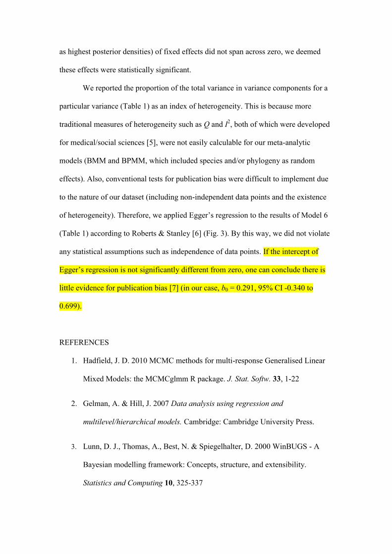
We reported the proportion of the total variance in variance components for a
particular variance (Table 1) as an index of heterogeneity. This is because more
traditional measures of heterogeneity such as Q and I2, both of which were developed
for medical/social sciences [5], were not easily calculable for our meta-analytic
models (BMM and BPMM, which included species and/or phylogeny as random
effects). Also, conventional tests for publication bias were difficult to implement due
to the nature of our dataset (including non-independent data points and the existence
of heterogeneity). Therefore, we applied Egger’s regression to the results of Model 6
(Table 1) according to Roberts & Stanley [6] (Fig. 3). By this way, we did not violate
any statistical assumptions such as independence of data points. If the intercept of
Egger’s regression is not significantly different from zero, one can conclude there is
little evidence for publication bias [7] (in our case, b0 = 0.291, 95% CI -0.340 to
0.699).
REFERENCES
1. Hadfield, J. D. 2010 MCMC methods for multi-response Generalised Linear
Mixed Models: the MCMCglmm R package. J. Stat. Softw. 33, 1-22
2. Gelman, A. & Hill, J. 2007 Data analysis using regression and
multilevel/hierarchical models. Cambridge: Cambridge University Press.
3. Lunn, D. J., Thomas, A., Best, N. & Spiegelhalter, D. 2000 WinBUGS - A
Bayesian modelling framework: Concepts, structure, and extensibility.
Statistics and Computing 10, 325-337

4. Gelman, A. & Rubin, D. B. 1992 Inference from iterative simulation using
multiple sequences (with discusiion). Statistical Science 7, 457-511.
5. Higgins, J. P. T., Thompson, S. G., Deeks, J. J. & Altman, D. G. 2003
Measuring inconsistency in meta-analyses. Brit. Med. J. 327, 557-560.
6. Robert, C. J. & Stanley, T. D. Meta-regression analysis: issues of publication
bias in economics. Oxford: Blackwell Publishing
7. Egger, M., Smith, G. D., Schneider, M. & Minder, C. 1997 Bias in meta-
analysis detected by a simple, graphical test. Brit. Med. J. 315, 629-634.

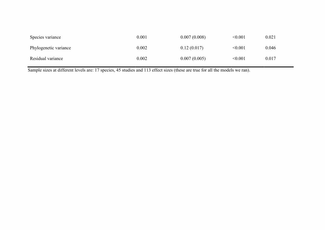
Table S1. Estimates from Bayesian mixed-effects meta-analysis (Model 1) and phylogenetic mixed-effects meta-analysis (Model 2) for the
relationship between male attractiveness and (SD: standard deviation of estimate, CI: credible interval).
Fixed effects Posterior mode Posterior mean (SD) Lower CI Upper CI
Model 1
Intercept (meta-analytic mean) 0.128 0.146 (0.034) 0.078 0.213
Model 2
Intercept (meta-analytic mean) 0.157 0.171 (0.070) 0.045 0.310
Random effects Posterior mode Posterior mean (SD) Lower CI Upper CI
Model 1
Study variance 0.001 0.008 (0.008) <0.001 0.023
Species variance 0.002 0.007 (0.009) <0.001 0.022
Residual variance 0.001 0.007 (0.006) <0.001 0.018
Model 2
Study variance 0.001 0.008 (0.007) <0.001 0.022
Species variance 0.001 0.007 (0.008) <0.001 0.021
Phylogenetic variance 0.002 0.12 (0.017) <0.001 0.046
Residual variance 0.002 0.007 (0.005) <0.001 0.017
Sample sizes at different levels are: 17 species, 45 studies and 113 effect sizes (these are true for all the models we ran).

Table S2. Estimates from Bayesian mixed-effects meta-regression analysis (Model 3) and phylogenetic mixed-effects meta-regression analysis
(Model 4) for the relationship between male attractiveness and female investment with the moderator, female traits (SD: standard deviation of a
parameter estimate, CI: credible interval).
Fixed effects Posterior mode Posterior mean (SD) Lower CI Upper CI
Model 3
Clutch size 0.113 0.118 (0.048) 0.025 0.208
Egg size 0.169 0.179 (0.054) 0.068 0.283
Feeding rate 0.259 0.278 (0.087) 0.105 0.444
Laying onsets 0.101 0.092 (0.075) -0.050 0.241
Yolk androgen 0.171 0.148 (0.063) 0.029 0.271
Immunity stimulants 0.055 0.070 (0.089) -0.108 0.238
Model 4
Clutch size 0.137 0.150 (0.082) <0.001 0.339
Egg size 0.182 0.211 (0.085) 0.048 0.381

Feeding rate 0.300 0.314 (0.113) 0.131 0.559
Laying onsets 0.131 0.122 (0.099) -0.081 0.307
Yolk androgen 0.224 0.176 (0.089) -0.023 0.332
Immunity stimulants 0.102 0.094 (0.108) -0.136 0.295
Random effects Posterior mode Posterior mean (SD) Lower CI Upper CI
Model 3
Study variance 0.001 0.008 (0.008) <0.001 0.023
Species variance 0.001 0.007 (0.009) <0.001 0.026
Residual variance 0.002 0.008 (0.006) 0.001 0.020
Model 4
Study variance 0.001 0.007 (0.006) <0.001 0.019
Species variance 0.001 0.007 (0.009) <0.001 0.022
Phylogenetic variance 0.001 0.014 (0.027) <0.001 0.051
Residual variance 0.002 0.008 (0.006) <0.001 0.021
Note that the intercepts were removed from Models 3 &4 for better interpretability.

Table S3. Estimates from Bayesian mixed-effects meta-regression analysis (Model 5) and phylogenetic mixed-effects meta-regression analysis
(Model 6) for the relationship between male attractiveness and female investment with the moderator, female traits, parental care types and their
interactions (SD: standard deviation of a parameter estimate, CI: credible interval).
Fixed effects Posterior mode Posterior mean (SD) Lower CI Upper CI
Model 5
Intercept (clutch size & both care) 0.108 0.133 (0.522) 0.030 0.230
Egg size (Δ between egg size & clutch size) 0.005 -0.002 (0.062) -0.120 0.121
Feeding rate (Δ between rate & clutch size) 0.198 0.140 (0.093) -0.049 0.311
Laying onset (Δ between onset & clutch size) -0.003 -0.044 (0.080) -0.195 0.111
Yolk androgen (Δ between androgen & clutch size) -0.054 -0.071 (0.078) -0.219 0.085
Immunity stimulants (Δ between immu. & clutch size) -0.141 -0.157 (0.119) -0.410 0.051
Female care (Δ between female care & both care) -0.058 -0.068 (0.111) -0.307 0.132
Egg size : Female care 0.226 0.258 (0.134) 0.018 0.541
Laying onset : Female care 0.116 -0.027 (0.311) -0.672 0.549

Yolk androgen : Female care 0.479 0.442 (0.171) 0.120 0.765
Immunity stimulants : Female care 0.254 0.279 (0.175) -0.056 0.620
Model 6
Intercept (clutch size & both care) 0.127 0.168 (0.096) -0.026 0.347
Egg size (Δ between egg size & clutch size) 0.006 -0.002 (0.062) -0.120 0.118
Feeding rate (Δ between rate & clutch size) 0.156 0.132 (0.092) -0.056 0.304
Laying onset (Δ between onset & clutch size) -0.034 -0.050 (0.077) -0.189 0.107
Yolk androgen (Δ between androgen & clutch size) -0.106 -0.072 (0.077) -0.223 0.079
Immunity stimulants (Δ between immu. & clutch size) -0.143 -0.162 (0.120) -0.374 0.088
Female care (Δ between female care & both care) -0.159 -0.109 (0.142) -0.400 0.148
Egg size : Female care 0.265 0.249 (0.135) 0.001 0.522
Laying onset : Female care -0.119 -0.044 (0.323) -0.644 0.606
Yolk androgen : Female care 0.464 0.436 (0.166) 0.141 0.794
Immunity stimulants : Female care 0.255 0.272 (0.174) -0.081 0.581
Random effects Posterior mode Posterior mean (SD) Lower CI Upper CI

Model 5
Study variance 0.002 0.009 (0.008) <0.001 0.025
Species variance 0.001 0.007 (0.008) <0.001 0.024
Residual variance 0.001 0.006 (0.005) <0.001 0.017
Model 6
Study variance 0.001 0.008 (0.008) <0.001 0.025
Species variance 0.001 0.007 (0.007) <0.001 0.021
Phylogenetic variance 0.001 0.012 (0.020) <0.001 0.047
Residual variance 0.002 0.005 (0.005) <0.001 0.015
The character Δ stands for ‘difference’.
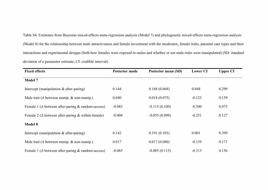
Table S4. Estimates from Bayesian mixed-effects meta-regression analysis (Model 7) and phylogenetic mixed-effects meta-regression analysis
(Model 8) for the relationship between male attractiveness and female investment with the moderator, female traits, parental care types and their
interactions and experimental designs (both how females were exposed to males and whether or not male traits were manipulated) (SD: standard
deviation of a parameter estimate, CI: credible interval).
Fixed effects Posterior mode Posterior mean (SD) Lower CI Upper CI
Model 7
Intercept (manipulation & after-paring) 0.144 0.168 (0.068) 0.048 0.299
Male trait (Δ between manip. & non-manip.) 0.040 0.018 (0.075) -0.123 0.159
Female 1 (Δ between after-paring & random-access) -0.083 -0.115 (0.100) -0.300 0.075
Female 2 (Δ between after-paring & within-female) -0.004 -0.055 (0.099) -0.251 0.127
Model 8
Intercept (manipulation & after-paring) 0.142 0.191 (0.103) 0.001 0.399
Male trait (Δ between manip. & non-manip.) 0.017 0.017 (0.080) -0.139 0.171
Female 1 (Δ between after-paring & random-access) -0.065 -0.085 (0.113) -0.313 0.156

Female 2 (Δ between after-paring & within-female) -0.045 -0.0224 (0.113) -0.248 0.202
Random effects Posterior mode Posterior mean (SD) Lower CI Upper CI
Model 7
Study variance 0.002 0.011 (0.010) <0.001 0.032
Species variance 0.001 0.009 (0.012) <0.001 0.031
Residual variance 0.001 0.006 (0.006) <0.001 0.018
Model 8
Study variance 0.002 0.011 (0.010) <0.001 0.032
Species variance 0.001 0.009 (0.015) <0.001 0.028
Phylogenetic variance 0.002 0.015 (0.026) <0.001 0.051
Residual variance 0.001 0.005 (0.005) <0.001 0.016
Note that fixed effects estimates included in Models 5 & 6 were omitted as qualitative results remain the exactly the same in the corresponding
models. The character Δ stands for ‘difference’.

Figure. S1. The topology of the phylogenetic tree used for Bayesian phylogenetic
mixed-effects meta-analysis (BPMM; Models 2, 4, 6, & 8 in Table 1).