Strategic Asset Valuation and Higher Stochastic … Asset Valuation and Higher Stochastic Moments:...

Journal of Contemporary Management

Submitted on 26/02/2015

Article ID: 1929-0128-2015-03-95-12

Gastón Milanesi, Gabriela Pesce, and Emilio El Alabi

~ 95 ~

Strategic Asset Valuation and Higher Stochastic Moments:

An Adjusted Black-Scholes Model

Dr. Gastón Milanesi (Correspondence author)

Business Administration Department, Universidad Nacional del Sur

San Andres 800, Bahia Blanca, Buenos Aires, 8000, ARGENTINA

Tel: +54-291-459-5132 (int. 1054) E-mail: [email protected]

Dr. Gabriela Pesce




Emilio El Alabi




Abstract: Strategic asset valuation is a complex problem which influences the decision making in

companies, such as decisions to differing or selling a project. Uncertainty takes over the manager

when defining the attributes of the density function representing values that could assume the asset

in the future. In this paper, we include not only its mean and variance, but also stochastic higher

moments of this function (asymmetry and kurtosis). This paper is original since we prove how

strategic decisions are subject to the impact of higher moments in the expanded value of assets. This

is why we include a detailed sensitivity analysis to clarify changes in valuation because of the

influence of asymmetry (ε) or kurtosis (κ) on the underlying asset distribution. Hence, we obtained

theoretical solutions to asset valuations that would have been impossible to solve.

Keywords: Strategic Asset; Asymmetry; Kurtosis; Edgeworth Expansion; Continuous Time; Real

Option; Firm Valuation; Black-Scholes Model

JEL Classifications: G32, M13, G13

1. Introduction

Real asset valuation is a complex problem that influences strategic decision making on firms

such as differing or selling a project. Uncertainty takes over the entrepreneur while defining density

function that represents different values that will assume the asset in the future. On this situation,

we do not only include its mean and variance, but also stochastic higher moments.

Milanesi, Pesce & El Alabi (2013) presents a solution in discrete time. This article offers a

solution to the mentioned problem in continuous time working on a case study. Therefore, this

work’s objective is to propose a technique to value strategic assets using the classic option valuation

model in continuous time (Black & Scholes, 1973) together with the Edgeworth expansion in order

ISSN: 1929-0128(Print); 1929-0136(Online) ©Academic Research Centre of Canada

~ 96 ~

to incorporate stochastic higher moments on the underlying distribution. Thus, we propose to adapt

the normal function and to test the model over the case study.

We structure the paper on the following manner: section 2 presents theoretical background

where we describe meanly what the Edgeworth expansion is and how it is adjusted to Black and

Scholes (BS). In section 3, we work with the Black-Scholes-Edgeworth (BSE) model applied as a

case study. From this point, we firstly estimate the implicit volatility curve, and then we value

different real options (differing, selling, and complex combined strategies). Lastly, we conclude on

the importance of utilizing this type of models to include extreme events in future scenarios of real

asset strategic values.

2. Theoretical Background

2.1 Edgeworth expansion

Jarrow and Rudd (1982) applied Edgeworth expansion on Schleher technique (1977) where the

real probability distribution Z(x) is approach by a different one called G(x). In statistics, this

technique is known as the Edgeworth expansion (Cramer, 1946; Kendall & Stuarts, 1977). The

expansion approaches a more complex probability distribution to a simpler alternative such as the

normal or lognormal distribution. This technique allows the expansion’s coefficient to depend on

the moments, either the original distribution or the approach one. Therefore, we obtained theoretical

solutions to asset valuations that would have been impossible to solve. From Jarrow and Rudd

(1982), and Baliero Filho and Rosenfeld (2004) as well, we contrast this methodology in order to

explain volatility smile1.

Following Baliero Filho and Rosenfeld (2004), we develop the expansion. Assume a series of

independent, identically distributed random variables (iid) x1, x2, ..., xn with mean μ and finite

variance σ2. On this case, the random variable is defined as (1):

Probability distribution of the random variable is obtained through an expansion on the

characteristic function distribution resulting in

for the normal distribution,

and where represents the underlying value at moment n. The characteristic function is expanded

the following manner (2):

(2)

Values indicate stochastic moments on the underlying distribution Sn. Here, first moment is

equal to and second moment is equal to . Baliero Filho and

Rosenfeld (2004) come up to the Edgeworth expansion (3):

(3)

This expression is valid until the order 1/n, asymmetry is defined as and kurtosis

, incorporating factors 1/n on this parameters. Function g(x) is the product between

1 It is an implicit volatility patron detected in numerous works (Rubinstein, 1994). It suggests that the

Black and Scholes option valuation model tends to undervalue options that are way in- or way out-of-the-money.

Journal of Contemporary Management, Vol. 4, No. 3

~ 97 ~

Gaussian distribution N(0,1) z(x) and the expression belongs to the expansion.

2.2 Black and Scholes model and the adjustment with the Edgeworth expansion

Financial and real assets returns’ distributions hardly ever adjust to the classic normal behavior

having asymmetry and weight on the extremes. New projects, technological developments, and

market innovation are characterized by the lack of comparable assets and the absence of price and

returns observations. Assuming the underlying stochastic process over the first two moments

(mean-variance) could generate errors in evaluating the real asset or the underlying financial asset.

Therefore, it is necessary to incorporate stochastic higher moments allowing a better valuation and

volatility estimation2.

Baliero and Rosenfeld (2004) model derivation starts from the asset growth rate defined as:

(4)

In this equation, r is the risk free rate, T is the time left until the option expires, σ is the

underlying asset volatility, ε is asymmetry, and κ is kurtosis. Having asymmetry =0 and kurtosis

κ=3 (normal), then μ=r. Thus, we obtain same solution as BS. Conventional expression of the BS

model for call options is:

(5)

where is the option theoretical value, is the underlying asset present value, is the

cumulative normal distribution of the variable , is the strike price, r is the risk free rate, and t

the expiration date3

. Variables and are estimated in the following manner:

and .

For the general case, the expression that determines the option expected value is:

(6)

where

is the call theoretical value, r is the risk free rate, T is the time horizon until

expiration, 0S the underlying asset market value on t=0, σ is volatility, K is the strike price, and g(x)

is the transformed function. The integral could be converted into a closed solution model for the

option valuation (Baliero Filho & Rosenfeld, 2004) resulting in a two-section divided equation: the

BS model and the Edgeworth expansion:

2 Stochastic moments in financial derivatives could be inferred from market prices. This allows to an

adjusted volatility measure. In valuation models in real options, moments could be sensitize presenting a range of values related to the strategic flexibility valued.

3 The expression is the expected present value related to the underlying asset in case that the

option ends in-the-money, being the risk adjusted probability that the underlying ends above

the exercise price at expiration. is the expected present value of the exercise price if the

options ends up in-the-money, being the risk adjusted probability that the option being

exercised. (Carmichael, Hersh & Parasu, 2011).


~ 98 ~

In the previous equation, is the call option value according to BS, r is the risk free rate, T

is the time horizon until expiration, 0S is the underlying asset market value in t=0, is volatility,

K is the strike price, u is the asset growth rate (equation 4), ε is asymmetry, κ is kurtosis, and

is the minimum value to guarantee that the integer from equation (6) be

positive. Variable is the same as 1d in the BS model with ε=0 and κ=3. In cases like this

(normality), the transformed model converges to BS. Same criterion follows the put option. To the

BS equation 0 1 21 1BS rT

oP V N d Ke N d , we add the Edgeworth expansion g(x),

0 0 ( )edge BSP P g x . We come up to the same result applying the put-call parity.

3. The Black-Scholes-Edgeworth (BSE) Model: An Application Case

3.1 Estimating the Implicit Volatility Curve

In order to illustrated how stochastic higher moments impact on the implicit utility curve, this

utility curve will be derived using equation (7) through an iterative process4. On this process, the

equation is equaled to the observed market price (Ct)5 to get implicit values related to deviation (σ),

asymmetry (ε), kurtosis (κ). Thus, we establish the following restrictions6: Ct ≥0; σ ≥ 0; -0,8≤ ε

≤0,8; 3≤ κ ≤5,4. The process starts establishing higher moments with value zero and volatility with

4 The iterative process is solved using Solver tool from Microsoft Excel ®. We define each cell where we

introduce the market price from equation (7) as an objective value. This is equal to the prime market value. Volatility, asymmetry, kurtosis, and risk free rate are cells to be changed.

5 On every model where variables are estimated implicitly, it is assumed that market values are correct. 6 Restrictions related to asymmetry and kurtosis, are defined according to the potential null values for

the function (Baliero Filho & Rosenfeld, 2004). These restrictions are defined by Solver in Microsoft Excel ®.


~ 99 ~

its implicit value7. Once we get the implicit values for the stochastic moments, we proceed to obtain

implicit volatility from the classic BS equation. To do this, we set again higher moments as ε=0;

κ=3.

We valued Facebook Inc. (FB) vanilla options listed in the National Association of Securities

Dealers Automated Quotation (NASDAQ). In order to use the variable estimation on a hypothetical

case of real option valuation, we selected contracts with expiration date on January, 15th, 2016 and

different exercise prices. Risk free rate belongs to a treasury bill with expiration in a year from t=0

being 0.16% annually8. Values on in-the-money option contracts are taken from Yahoo Finance

9

which expire on February, 6th, 2016. On Annex 1, we expose data related to the valued contract.

The following table compares implicit volatility taken from BS and BSE models. First column are

strike prices for our contracts. Second and third columns are implicit volatility from BS and BSE

models. Fourth and fifth columns are asymmetry and kurtosis implicit on BSE model. Sixth column

is the portion of price related to the BS model (having =0, =3 and BSE volatility). Seventh

column is the magnitude of price explained by the expansion. Eighth column are market prices.

Finally, ninth column is the percentage that the expansion represents on price.

Table 1. Implicit values are obtained from the iterative process related to equation (7)

Strike σ (i) BS σ (i) BSE BS E Price E/Price

13.00 86.51% 83.60% 0.0011 3.00 62.72 0.03 62.75 0.05%

15.00 126.87% 79.22% 0.0558 3.15 60.75 1.45 62.20 2.33%

18.00 73.25% 72.96% -0.0383 2.91 57.79 -0.79 57.00 -1.39%

20.00 88.28% 68.36% 0.0368 3.08 55.81 0.64 56.45 1.14%

23.00 49.76% 63.24% -0.0142 2.97 52.85 -0.20 52.65 -0.38%

25.00 83.14% 61.92% 0.0751 3.13 50.93 0.97 51.90 1.86%

30.00 65.28% 55.29% 0.0543 3.07 46.05 0.50 46.55 1.08%

33.00 83.05% 55.47% 0.2918 3.29 43.32 2.31 45.63 5.06%

35.00 45.74% 52.68% -0.0496 2.99 41.36 -0.36 41.00 -0.89%

38.00 71.05% 57.06% 0.1981 2.95 39.11 1.49 40.60 3.67%

40.00 42.15% 46.91% -0.0585 3.04 36.53 -0.33 36.20 -0.92%

43.00 47.40% 46.54% 0.0152 2.98 33.91 0.09 34.00 0.25%

45.00 47.44% 45.36% 0.0420 2.93 32.11 0.24 32.35 0.73%

47.00 31.39% 36.52% -0.0948 3.20 29.51 -0.41 29.10 -1.41%

50.00 38.90% 39.27% -0.0081 3.03 27.28 -0.05 27.23 -0.17%

52.50 37.33% 37.30% 0.0006 3.00 25.00 0.00 25.00 0.02%

55.00 36.66% 36.68% -0.0003 3.00 22.95 0.00 22.95 -0.01%

57.50 35.62% 35.79% -0.0028 3.03 20.93 -0.03 20.90 -0.15%

60.00 35.02% 35.10% 0.0000 3.02 19.02 -0.02 19.00 -0.08%

7 We obtain implicit volatility using Microsoft Excel ® where we define the BS cell with the market value

to change volatility. Market prices are taken from http://finance.yahoo.com/q/op?s=FB&date= 1452816000.

8 We obtained data from the Federal Reserve website: http://www.federalreserve.gov/releases/h15 cuadro h.15 interest rate on 2/2015.

9 Yahoo Finance website: http://finance.yahoo.com/q/op?s=FB&date=1452816000


~ 100 ~

62.50 34.50% 34.52% -0.0002 3.01 17.21 -0.01 17.20 -0.04%

65.00 33.19% 33.23% -0.0001 3.01 15.31 -0.01 15.30 -0.06%

67.50 31.81% 31.98% 0.0001 3.01 13.46 -0.01 13.45 -0.05%

70.00 32.38% 32.37% 0.0000 3.00 12.20 0.00 12.20 0.00%

72.50 31.89% 31.89% 0.0000 3.00 10.78 0.00 10.78 0.00%

75.00 31.36% 31.36% 0.0001 3.00 9.45 0.00 9.45 0.00%

77.50 30.86% 30.86% -0.0002 3.00 8.23 0.00 8.23 0.00%

80.00 30.35% 30.35% -0.0005 3.00 7.11 0.00 7.11 -0.01%

82.50 30.39% 30.38% 0.0006 3.00 6.25 0.00 6.25 0.01%

85.00 29.61% 29.61% -0.0010 3.00 5.25 0.00 5.25 -0.03%

87.50 29.92% 29.91% 0.0021 3.00 4.65 0.00 4.65 0.08%

90.00 29.39% 29.39% -0.0001 3.00 3.90 0.00 3.90 0.00%

95.00 28.82% 28.83% -0.0008 3.00 2.77 0.00 2.77 -0.13%

100.00 28.57% 28.61% -0.0007 3.01 1.99 -0.01 1.98 -0.34%

105.00 28.61% 28.65% 0.0000 3.01 1.45 -0.01 1.44 -0.45%

110.00 29.26% 29.13% -0.0020 2.98 1.11 0.02 1.13 1.62%

115.00 28.85% 28.84% -0.0001 3.00 0.77 0.00 0.77 0.07%

120.00 28.40% 28.56% 0.0061 3.01 0.53 -0.02 0.51 -2.97%

125.00 28.80% 28.86% 0.0023 3.00 0.40 -0.01 0.39 -1.33%

130.00 29.01% 29.10% 0.0022 3.00 0.30 -0.01 0.29 -1.93%

135.00 29.71% 29.39% -0.0053 3.01 0.22 0.02 0.24 6.35%

140.00 29.61% 29.59% -0.0002 3.00 0.17 0.00 0.17 0.47%

145.00 32.99% 30.85% -0.0262 3.05 0.16 0.10 0.26 36.61%

150.00 30.10% 31.03% 0.0066 2.99 0.13 2.99 3.11 95.93%

155.00 32.36% 31.69% -0.0045 3.01 0.11 0.02 0.13 15.08%

Data source: Own elaboration

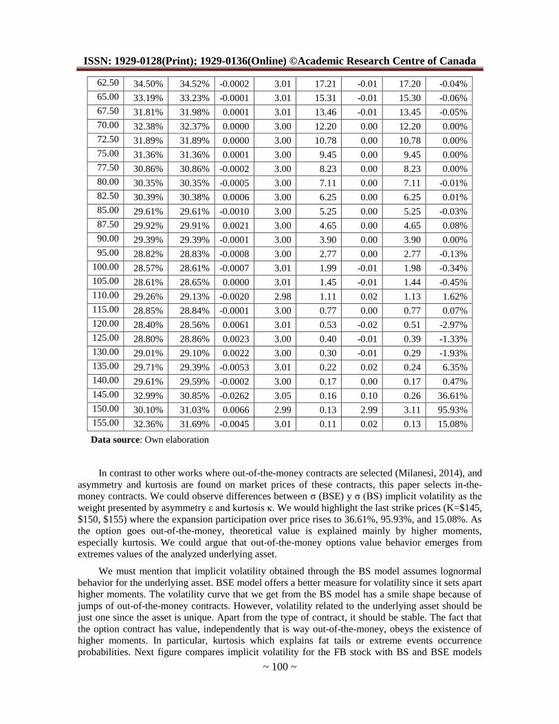
In contrast to other works where out-of-the-money contracts are selected (Milanesi, 2014), and

asymmetry and kurtosis are found on market prices of these contracts, this paper selects in-the-

money contracts. We could observe differences between σ (BSE) y σ (BS) implicit volatility as the

weight presented by asymmetry ε and kurtosis κ. We would highlight the last strike prices (K=$145,

$150, $155) where the expansion participation over price rises to 36.61%, 95.93%, and 15.08%. As

the option goes out-of-the-money, theoretical value is explained mainly by higher moments,

especially kurtosis. We could argue that out-of-the-money options value behavior emerges from

extremes values of the analyzed underlying asset.

We must mention that implicit volatility obtained through the BS model assumes lognormal

behavior for the underlying asset. BSE model offers a better measure for volatility since it sets apart

higher moments. The volatility curve that we get from the BS model has a smile shape because of

jumps of out-of-the-money contracts. However, volatility related to the underlying asset should be

just one since the asset is unique. Apart from the type of contract, it should be stable. The fact that

the option contract has value, independently that is way out-of-the-money, obeys the existence of

higher moments. In particular, kurtosis which explains fat tails or extreme events occurrence

probabilities. Next figure compares implicit volatility for the FB stock with BS and BSE models


~ 101 ~

according to table 1 above.

Figure 1. Implicit volatility for BS and BSE derivate from call option contracts for FB

(own elaboration)

We could appreciate a higher flattening on the curve estimated with the BSE related to the

traditional model. BSE separates higher moments of implicit volatility and, as a consequence, the

softer behavior of the implicit volatility curve. We must consider this while applying real options in

valuing strategic flexibility on investment projects.

3.2 Real Options and the BSE Model: Analysis of differing, Selling, and Combined Options

In order to illustrate differences while valuating options between BS and BSE models, we

assume that the same firm is planning on developing a new app to be commercialized. The project

has two stages: the pilot stage and the commercial stage where the beginning of the commercial

stage is conditioned by the final results of the pilot stage. First phase lasts five years (t=5). On the

second phase, we estimate the present value of the benefits, $4,375 (thousands) with a

$1,345 (thousands) deviation through a series of scenarios. The firm’s cost of capital (WACC) is

assumed on 10.5% and the risk free rate is 5.5% annually. The investment needed for the second

phase (commercialization) to be made on the fifth year is $5,000 (thousands), risk free.

If the project is valued by the traditional net present value (NPV) approach, we get:

$2,588.05 (thousands); 3,797.86 (thousands). Therefore, = -$1,209.81 (thousands). The obtained result drives us to reject the project

since efforts in research and development (R&D) made during the first stage will not result in

favorable outcomes during the second stage. Consequently, we will not initiate the pilot stage.

However, it does not consider the added value for having flexibility during the project since it

assumes that the investment is irreversible and inflexible. On this case, we assume that compromise

of investing on the second stage t=5 is assumed to be on t=0. Thus, strategic flexibility must be

quantified using real option valuation models. Options contained in the project are: (a) to differ the

investment until moment t=5 waiting for more information related to the market evolution once

introducing this new app; (b) to develop the project and investing and then, on t=5, selling the

project in $2,500 (thousands) if the non-favorable evolution occurs; (c) to combine the option of

0%

20%

40%

60%

80%

100%

120%

140%

13

.00

18

.00

23

.00

30

.00

35

.00

40

.00

45

.00

50

.00

55

.00

60

.00

65

.00

70

.00

75

.00

80

.00

85

.00

90

.00

10

0.0

0

11

0.0

0

12

0.0

0

13

0.0

0

14

0.0

0

15

0.0

0

Vo

lati

lity

Strike price

Implied Sigma BS

sigma BSE


~ 102 ~

differ and then investment or selling the project. The first alternative is similar to a call, the second

to a put, and the third to a strangle which is a strategy that unifies investment (buying) with the

possibility of abandoning (selling).

The objective is to determine strategic flexibility value with expanded real option models.

First, expanded value (EV) is equal to the traditional value (NPV) plus the value of the real options

(RO):

(8)

On this case, values related to differing, selling, and the combination are determined by the

following parameters: underlying present value

; strike price for the differing option ; selling option ; risk free

rate ; and time until exercise for both options . Volatility expressed as a percentage

is obtained by clearing10

from the expression

(Wilmott, Howison & Dewynne, 1995) where .

The value of the differing option according to BS (ε =0; κ=3) comes up from the following

expression: with these parameters:

The strategic value is $44.76

(thousands), thus, differing option value goes up to $1,254.57 (thousands) indicating the

convenience to invest in phase 1, instead of not investing, while waiting to new information on t=5

to complete phase 2.

In the selling option, we use the expression of the put option on BS: (ε=0; κ=3); with parameters:

. The strategic value is

$52.01 (thousands), the abandoning or selling option goes up to $1,261.81 (thousands).

Finally, the combined strategy offers the project an EV of $96.67 (thousands) which is the sum

of strategic values related to buying and selling options. The EV is $1,306.58 (thousands) which is

the feasibility of making R&D on the first stage and then, on t=5, making the investment and

commercializing or, contrarily, transferring the app license. If the previsions actually occur, selling

the license is more profitable than commercializing the app.

As we previously mentioned, this type of projects hardly ever present a lognormal behavior. In

fact, its success probability depends on extreme events. The convenience of transferring the license

or investing and commercializing will depend on the stochastic behavior of the underlying asset.

Therefore, we must incorporate stochastic higher moments.

We used the defined equations in section 2 in order to value differing and selling options

contained in the project considering stochastic higher moments. Thus, while analyzing potential

values for the options, we proceed to sensitize higher moments: asymmetry ε=[-0,7; 0,7] and

kurtosis κ=[3; 5,4]. Volatility remained fixed. On the following tables, we expose values related to

the project strategic value with the differing option (table 2), the selling option (table 3), and the

combined differing and selling option (table 4).

On these tables, we highlight project strategic values in cases where we assume normality. The

higher the positive asymmetry and kurtosis (meso-kurtosis), the value of the differing and

abandoning options goes up. On the case of negative asymmetries, they counteract the higher value

that is obtained by the fourth stochastic moment. Tables focus on the impact of kurtosis on the

differing value (table 2), if it is compared to selling option (table 3). In case the project allows us to

10 Volatility is obtained by iterating the expression with the search objective function from MS Excel ®.


~ 103 ~

implement both strategies concomitantly, values are exposed on table 4. These values come up from

summing up values on tables 2 and 3.

Table 2. Sensitivity of differing option value according on asymmetry and kurtosis (Own elaboration)

ε \ κ 3.0 3.3 3.5 3.8 4.0 4.3 4.5 4.8 5.0 5.3 5.5

0.7 76.61 79.47 81.37 84.21 86.11 88.95 90.84 93.68 95.57 98.40 100.2

0.6 71.08 73.93 75.84 78.69 80.59 83.44 85.34 88.18 90.07 92.91 94.80

0.5 65.87 68.73 70.64 73.50 75.40 78.26 80.16 83.01 84.90 87.74 89.64

0.4 60.99 63.86 65.77 68.63 70.54 73.40 75.30 78.16 80.06 82.91 84.81

0.3 56.43 59.31 61.23 64.10 66.01 68.87 70.78 73.64 75.55 78.40 80.30

0.2 52.21 55.09 57.01 59.89 61.80 64.68 66.59 69.45 71.36 74.22 76.13

0.1 48.32 51.21 53.13 56.01 57.93 60.81 62.72 65.59 67.51 70.37 72.28

0.0 44.77 47.66 49.58 52.47 54.39 57.27 59.19 62.07 63.98 66.85 68.77

-0.1 41.54 44.44 46.36 49.26 51.18 54.07 55.99 58.87 60.79 63.67 65.58

-0.2 38.65 41.55 43.48 46.38 48.31 51.20 53.12 56.01 57.93 60.81 62.73

-0.3 36.09 39.00 40.93 43.83 45.76 48.66 50.59 53.48 55.40 58.29 60.21

-0.4 33.87 36.78 38.72 41.62 43.56 46.46 48.39 51.28 53.21 56.10 58.03

-0.5 31.99 34.90 36.84 39.75 41.69 44.59 46.52 49.42 51.35 54.25 56.18

-0.6 30.44 33.36 35.30 38.21 40.15 43.06 45.00 47.90 49.83 52.73 54.66

-0.7 29.24 32.16 34.10 37.02 38.96 41.87 43.81 46.72 48.65 51.55 53.49

Table 3. Sensitivity of selling option value according on asymmetry and kurtosis (Own elaboration)

ε \ κ 3.0 3.3 3.5 3.8 4.0 4.3 4.5 4.8 5.0 5.3 5.5

0.7 59.38 59.65 59.82 60.08 60.26 60.52 60.70 60.97 61.14 61.41 61.58

0.6 58.28 58.54 58.72 58.98 59.15 59.42 59.59 59.86 60.03 60.30 60.47

0.5 57.19 57.45 57.63 57.89 58.06 58.33 58.50 58.77 58.94 59.20 59.38

0.4 56.12 56.38 56.56 56.82 56.99 57.26 57.43 57.69 57.87 58.13 58.31

0.3 55.07 55.33 55.50 55.76 55.94 56.20 56.38 56.64 56.81 57.07 57.25

0.2 54.03 54.29 54.47 54.73 54.90 55.16 55.34 55.60 55.77 56.03 56.21

0.1 53.01 53.27 53.44 53.71 53.88 54.14 54.31 54.57 54.75 55.01 55.18

0.0 52.01 52.27 52.44 52.70 52.87 53.13 53.31 53.57 53.74 54.00 54.18

-0.1 51.02 51.28 51.45 51.71 51.88 52.14 52.31 52.57 52.75 53.01 53.18

-0.2 50.04 50.30 50.47 50.73 50.90 51.16 51.34 51.60 51.77 52.03 52.20

-0.3 49.08 49.34 49.51 49.77 49.94 50.20 50.37 50.63 50.81 51.07 51.24

-0.4 48.13 48.39 48.56 48.82 48.99 49.25 49.42 49.68 49.86 50.12 50.29

-0.5 47.20 47.45 47.63 47.88 48.06 48.31 48.49 48.75 48.92 49.18 49.35

-0.6 46.27 46.53 46.70 46.96 47.13 47.39 47.56 47.82 48.00 48.25 48.43

-0.7 45.36 45.62 45.79 46.05 46.22 46.48 46.65 46.91 47.08 47.34 47.52

If the project offers an exclusionary strategy (differing-investing or selling), and we assume

normality on the underlying behavior, it is clear that if predictions on t=0 actually occur, the option

to be exercised on t=5 is the selling one. However, if the underlying asset does not follow a


~ 104 ~

stochastic normal behavior, the selected strategy will depend on the impact of moments in value.

From tables 2 and 3, we are able to build the following table where we present the decision to be

making on each pair (ε; κ).

Table 4. Sensitivity of strangle strategy value according on asymmetry and kurtosis (Own elaboration)

ε \ κ 3.0 3.3 3.5 3.8 4.0 4.3 4.5 4.8 5.0 5.3 5.5

0.7 135.99 139.11 141.19 144.30 146.37 149.47 151.54 154.64 156.71 159.80 161.87

0.6 129.35 132.47 134.55 137.67 139.75 142.86 144.93 148.04 150.10 153.20 155.27

0.5 123.06 126.18 128.27 131.39 133.47 136.58 138.66 141.77 143.84 146.95 149.02

0.4 117.11 120.24 122.32 125.45 127.53 130.66 132.74 135.85 137.93 141.04 143.11

0.3 111.50 114.64 116.73 119.86 121.95 125.07 127.16 130.28 132.36 135.48 137.55

0.2 106.24 109.39 111.48 114.62 116.71 119.84 121.92 125.05 127.13 130.26 132.34

0.1 101.33 104.48 106.58 109.72 111.81 114.95 117.04 120.17 122.26 125.38 127.47

0.0 96.77 99.92 102.02 105.17 107.26 110.40 112.50 115.63 117.72 120.85 122.94

-0.1 92.56 95.71 97.81 100.96 103.06 106.21 108.30 111.44 113.54 116.67 118.76

-0.2 88.69 91.85 93.95 97.11 99.21 102.36 104.46 107.60 109.70 112.84 114.93

-0.3 85.17 88.33 90.44 93.60 95.71 98.86 100.96 104.11 106.21 109.35 111.45

-0.4 82.00 85.17 87.28 90.44 92.55 95.71 97.81 100.97 103.07 106.22 108.31

-0.5 79.18 82.36 84.47 87.63 89.74 92.91 95.01 98.17 100.27 103.43 105.53

-0.6 76.72 79.89 82.01 85.18 87.29 90.45 92.56 95.72 97.83 100.99 103.09

-0.7 74.60 77.78 79.89 83.07 85.18 88.35 90.46 93.63 95.74 98.90 101.00

Table 5. Sensitivity about selling or differing according on asymmetry and kurtosis (Own elaboration)

ε \ κ 3.0 3.3 3.5 3.8 4.0 4.3 4.5 4.8 5.0 5.3 5.5

0.7 differ differ differ differ differ differ differ differ differ differ differ





0.2 sell differ differ differ differ differ differ differ differ differ differ

0.1 sell sell sell differ differ differ differ differ differ differ differ

0 sell sell sell sell differ differ differ differ differ differ differ

-0.1 sell sell sell sell sell differ differ differ differ differ differ

-0.2 sell sell sell sell sell differ differ differ differ differ differ

-0.3 sell sell sell sell sell sell differ differ differ differ differ

-0.4 sell sell sell sell sell sell sell differ differ differ differ



-0.7 sell sell sell sell sell sell sell sell differ differ differ


~ 105 ~

4. Conclusion

Financial and real assets returns’ distributions hardly ever adjust to the classic normal behavior

having asymmetry and weight on the extremes. This characteristic makes valuation a complex

problem which influences the strategic decision making in companies, such as decisions to expand,

to differ, or to sell a project.

This paper has proposed valuing strategic assets using real option theory making adjustments

that allow us to abandon the assumption of normal returns in continuous time. This technique

permits the expansion’s coefficient to depend also on the higher moments (asymmetry and

kurtosis), either the original distribution or the approached one. Therefore, we obtained theoretical

solutions to asset valuations that would have been difficult to solve.

Thus, this paper proposes to valuate this type of entrepreneurships using real options theory

making adjustments that allow us to abandon the assumption of normal returns in continuous time.

This technique permits the expansion’s coefficient to depend also on the higher moments, either the

original distribution or the approach one. Therefore, we presented theoretical results to valuation

difficulties that would have been impossible to approach.

References

[1] Baliero Filho, R. & Rosenfeld, R. (2004). "Testing Option Pricing with Edgeworth Expansion",

Physica A: Statistical Mechanis and Its Application, 344(3): 484-490.

[2] Black, F. & Scholes, M. (1973). "The pricing of options and corporate liabilities", Journal of

Political Economy, 81(3): 637-654.

[3] Carmichael, D., Hersh, A. & Parasu, P. (2011). "Real Options Estimate Using Probabilistic Present

Worth Analysis", The Engineering Economist, 56(4): 295-320.

[4] Cramer, H. (1946). Mathematical Methods for Statistics. Princeton, NJ: Princeton University Press.

[5] Jarrow, R. & Rudd, A. (1982). "Aproximate option valuation for arbitrary stochastic processes",

Journal of Financial Economics, 10(3): 347-369.

[6] Kendall, M. & Stuarts, A. (1977). The Advanced Theory of Statistics: Vol.1 Distribution Theory.

New York: Mcmillan.

[7] Milanesi, G. (2014). "Momentos estocásticos de orden superior y la estimación de la volatilidad

implícita: aplicación de la expansión de Edgeworth en el modelo Black-Scholes", Estudios

Gerenciales, 30(133): 336–342.

[8] Milanesi, G., Pesce, G. & El Alabi, E. (2013). "Technology-based startup valuation using real

options with Edgeworth expansion", Journal of Finance and Accounting, 1(2): 54-61.

[9] Rubinstein, M. (1994). "Implied Binomial Trees", Journal of Finance, 49(3): 771-818.

[10] Rubinstein, M. (1998). "Edgeworth Binomial Trees", Journal of Derivatives, 5(3): 20-27.

[11] Schleher, D. (1977). "Generalized Gram-Charlier series with application to the sum of log-normal",

IEEE Transactions on Information Theory, 23(2): 275-280.

Annex: Data published on Yahoo Finance. Call option for Facebook, Inc.

Expiring on January, 15th, 2016. (Own elaboration)

Strike Contract Last Bid Ask

13.00 FB160115C00013000 62.75 62.45 63.05

15.00 FB160115C00015000 62.20 60.45 61.10

18.00 FB160115C00018000 57.00 57.50 58.15

20.00 FB160115C00020000 56.45 55.50 56.15

http://finance.yahoo.com/q/op?s=FB&strike=15.00



http://finance.yahoo.com/q?s=FB160115C00020000


~ 106 ~

23.00 FB160115C00023000 52.65 52.55 53.20

25.00 FB160115C00025000 51.90 50.60 51.25

30.00 FB160115C00030000 46.55 45.70 46.35

33.00 FB160115C00033000 45.63 42.75 43.40

35.00 FB160115C00035000 41.00 40.80 41.45

38.00 FB160115C00038000 40.60 37.90 38.60

40.00 FB160115C00040000 36.20 36.00 36.70

43.00 FB160115C00043000 34.00 33.20 33.85

45.00 FB160115C00045000 32.35 31.35 31.90

47.00 FB160115C00047000 29.10 29.55 30.05

50.00 FB160115C00050000 27.23 26.85 27.35

52.50 FB160115C00052500 25.00 24.70 25.00

55.00 FB160115C00055000 22.95 22.65 22.95

57.50 FB160115C00057500 20.90 20.65 21.05

60.00 FB160115C00060000 19.00 18.70 19.10

62.50 FB160115C00062500 17.20 16.85 17.25

65.00 FB160115C00065000 15.30 15.10 15.45

67.50 FB160115C00067500 13.45 13.55 13.70

70.00 FB160115C00070000 12.20 12.00 12.15

72.50 FB160115C00072500 10.78 10.55 10.75

75.00 FB160115C00075000 9.45 9.45 9.50

77.50 FB160115C00077500 8.23 8.10 8.25

80.00 FB160115C00080000 7.11 7.05 7.15

82.50 FB160115C00082500 6.25 6.00 6.20

85.00 FB160115C00085000 5.25 5.20 5.30

87.50 FB160115C00087500 4.65 4.40 4.55

90.00 FB160115C00090000 3.90 3.75 3.90

95.00 FB160115C00095000 2.77 2.70 2.80

100.00 FB160115C00100000 1.98 1.93 2.02

105.00 FB160115C00105000 1.44 1.43 1.47

110.00 FB160115C00110000 1.13 0.96 1.06

115.00 FB160115C00115000 0.77 0.68 0.77

120.00 FB160115C00120000 0.51 0.47 0.55

125.00 FB160115C00125000 0.39 0.35 0.40

130.00 FB160115C00130000 0.29 0.25 0.30

135.00 FB160115C00135000 0.24 0.18 0.22

140.00 FB160115C00140000 0.17 0.15 0.17

145.00 FB160115C00145000 0.26 0.10 0.15

150.00 FB160115C00150000 0.10 0.06 0.13

155.00 FB160115C00155000 0.13 0.06 0.11

















































































Strategic Asset Valuation and Higher Stochastic … Asset Valuation and Higher Stochastic Moments:...

Documents

Transcript of Strategic Asset Valuation and Higher Stochastic … Asset Valuation and Higher Stochastic Moments:...