Storage Management in Wireless Sensor Networks

Sameer Tilak†, Nael Abu-Ghazaleh† and Wendi B. Heinzelman‡

†Department of Computer ScienceBinghamton UniversityBinghamton, NY, USA

‡Department of Electrical and Computer EngineeringUniversity of Rochester

Rochester, NY, USA

March 5, 2006

Abstract

Storage management is an area of sensor network research that is starting to attract atten-tion. The need for storage management arises primarily in the class of sensor networks whereinformation collected by the sensors is not relayed to observers in real-time (e.g., scientificmonitoring applications). In such applications, the data must be stored, at least temporarily,within the network until it is later collected by an observer(or until it ceases to be useful).Therefore, storage becomes a primary resource which, in addition to energy, determines theuseful lifetime and coverage of the network.

This chapter overviews issues and opportunities in storagemanagement for sensor net-works. We first motivate the need for storage management by overviewing sensor networkapplications that require storage management. We then discuss how the application character-istics and various resource constraints influence the design of storage management techniques.More specifically, we break down the storage management problem into the following compo-nents: (1) system support for storage management; (2) collaborative storage; and (3) indexingand retrieval. We then highlight the problems and issues in each of these components of storagemanagement, and we describe proposed solutions.

Keywords - Storage management, Collaborative storage, Indexing andretrieval, Memory,Non-real-time applications

1

1 Introduction

Wireless Sensor Networks (WSNs) hold the promise of revolutionizing sensing across a range ofcivil, scientific, military and industrial applications. However, many battery-operated sensors haveconstraints such as limited energy, computational ability, and storage capacity, and thus protocolsmust be designed to deal efficiently with these limited resources in order to maximize the datacoverage and useful lifetime of the network.

Storage management is an area of sensor network research that is starting to attract attention.The need for storage management arises primarily in the class of sensor networks where informa-tion collected by the sensors is not relayed to observers in real-time. In such applications, the datamust be stored, at least temporarily, within the network until it is later collected by an observer (oruntil it ceases to be useful). An example of this type of application is scientific monitoring, wherethe sensors are deployed to collect detailed information about a phenomenon for later playback andanalysis. Another example is that of sensors that collect data that is later accessed by dynamicallygenerated queries from users. In these types of applications, data must be stored in the network,and thus storage becomes a primary resource which, in addition to energy, determines the usefullifetime and coverage of the network.

With the knowledge of the relevant application and system characteristics, a set of goals forsensor network storage management can be determined. Theserequirements are: (1) minimizingstorage size to maximize coverage/data retention; (2) minimizing energy; (3) supporting efficientquery execution on the stored data (note that in the reachback method where all the data mustbe sent to the observer, query execution is simply the transfer of the data to the observer); and(4) providing efficient data management under constrained storage. Several approaches to storagemanagement have been proposed to meet the above requirements, with most approaches involvinga tradeoff among these different goals.

One basic storage management approach is to buffer the data locally at the sensors that collectthem. However, such an approach does not capitalize on the spatial correlation of data amongneighboring sensors to reduce the overall size of the storeddata (the property that makes dataaggregation possible [11]). Collaborative storage management, on the other hand, can provide thefollowing advantages over a simple buffering technique.

• More efficient storage allows the network to continue storing data for a longer time withoutexhausting storage space.

• Load balancing is possible. If the rate of data generation isnot uniform at the sensors (e.g.,in the case where a localized event causes neighboring sensors to collect data more aggres-sively), some sensors may run out of storage space while space remains available at others.In such a case, it is important for the sensors to collaborateto achieve load balancing forstorage to avoid or delay data loss due to insufficient local storage.

• Dynamic, localized reconfiguration of the network (such as adjusting sampling frequenciesof sensors based on estimated data redundancy and current resources) is possible.

Thus, collaborative storage is often better able to meet thegoals of storage management.

2

This chapter overviews issues and opportunities in storagemanagement for sensor networks.We first motivate the need for storage management by overviewing sensor network applicationsthat require storage management. We then discuss how the application characteristics and variousresource constraints influence the design of storage management techniques. Application charac-teristics define what data is useful and how the data will eventually be accessed; these featureshave significant implications on storage protocol design. In addition, hardware characteristicsdetermine the capabilities of the system and the energy efficiency of the storage protocols. Weoverview the characteristics of flash memory, the prevalentstorage technology in sensor networks,and we compare the cost of storage to that of computation and communication to establish the ba-sic data manipulation costs using current technologies forsubsequent tradeoff analyses. Then, as acase study, we discuss the design and implementation of the matchbox file system, which supportsmote based applications.

2 Motivation – Application Classes

In this section, the storage management problem is motivated by describing two application classesthat require effective use of storage resources. In general, storage is required whenever data is notrelayed to observers outside the network in real-time; the data must be stored by the sensors untilit is collected or discarded (it ceases to be useful, or it is sacrificed/compressed to make room formore important data). The following two applications illustrate different situations where such arequirement arises.

2.1 Scientific Monitoring – Playback Analysis

In scientific monitoring applications, the sensor network is deployed to collect data. This datais not of real-time interest; it is collected for later analysis to provide an understanding of someon-going phenomenon. Consider a wildlife tracking sensor network that scientists could use tounderstand the social behavior and migratory patterns of a species. Suppose sensors are deployedin a forest and collect data about nearby animals. In such an application, the sensors may nothave an estimate regarding the observer’s schedule for accessing the data. Furthermore, the datageneration rate at the sensors may be unpredictable, as it depends on the observed activity, and thesensor density may also be non-uniform [5]. The observer would like the network to preserve thecollected data samples, and the collection time should be small since the observer may not be inrange of the sensors for very long. An example of such a network is the ZebraNet project [13].

Scientists (observers) collect the data by driving around the monitored habitat, receiving in-formation from sensors as they come in range with them. Alternatively, the data may be relayedby the sensors in a multi-hop fashion towards the observer. Data collection is not pre-planned:it might be unpredictable and infrequent. However, the data“query” model is limited (one timecollection in a known fashion). This information about dataaccess patterns may be exploited; forexample, data may be stored at sensors closer to the observer. The long term availability of thedata allows aggregation/compression that can be significantly more efficient than that achieved byreal-time data collection sensor networks.

3

This type of situation also occurs in sensor networks that report their data in near real-timewhen the network becomes partitioned. For example, in the Remote Ecological Micro-Sensor Net-work [22], remote visual surveillance of federally listed rare and endangered plants is conducted.This project aims to provide near-real-time monitoring of important events, such as visitation bypollinators and consumption by herbivores, along with monitoring a number of weather conditionsand events. Sensors are placed in different habitats, ranging from scattered low shrubs to densetropical forests. Environmental conditions can be severe;e.g., some locations frequently freeze. Insuch applications, network partitioning (relay nodes becoming unavailable) may occur due to theextreme physical conditions (e.g., deep freeze). Important events that occur during disconnectionperiods should be recorded and reported once the connectionis reestablished. Effective storagemanagement is needed to maximize the partitioning time thatcan be tolerated without loss of data.

2.2 Augmented Reality – Multiple Observers, Dynamic Queries

Consider a sensor network that is deployed in a military scenario and collects information aboutnearby activity. The data is queried dynamically by soldiers to help with mission goals or withavoiding sources of danger, and by commanders to assess the progress of the mission. The querieddata is both real-time as well as long-term data about enemy activity (e.g., to answer a questionsuch as where are the supply lines). Thus, data must be storedat the sensors to enable queries thatspan temporally long periods, such as days or even months. One can envision similar applicationswith sensor networks deployed in other contexts that answerquestions about the environment usingboth real-time as well as recent or even historical data. Thedata is stored at the sensors and used,perhaps collaboratively, to answer queries.

In addition to efficiently using data storage to allow the sensor network to retain more data andhigher resolution data, one of the issues in this application is effective indexing and retrieval of thedata. While the data may be addressed by content (e.g., searching for information about a certaintype of vehicle), since the observers do not know where the data are stored, or even what data exist,the queries can be quite inefficient. Furthermore, data may be accessed multiple times, by differentobservers. Efficient indexing and retrieval of the data is desirable.

3 Preliminaries: Design Considerations, Goals and StorageMan-agement Components

The applications described in the previous section provideinsight into the range of issues that mustbe addressed to achieve effective storage management. In this section, these issues are describedmore directly. We first outline the factors that influence thedesign of storage management andthen discuss the design goals of such a system. We also break the storage management probleminto different components that require efficient protocols.

4

3.1 Design Considerations

Energy is a precious resource in all wireless micro-sensor networks; when the battery energy at asensor expires, the node ceases to be useful. Therefore, preserving energy is a primary concernthat permeates all aspects of sensor network design and operation. For storage bound applications,there is an additional finite resource: the available storage at the sensors. Once the available storagespace is exhausted, a sensor can no longer collect and store data locally; the sensors that have runout of storage space cease to be useful. Thus, a sensor network’s utility is bound by two resources:its available energy and its available storage space. Effective storage management protocols mustbalance these two resources to prolong the network’s usefullifetime.

The two limiting resources – storage and energy – are fundamentally different from each other.Specifically, storage is re-assignable while energy is not:a node may free up some storage spaceby deleting or compressing data. Furthermore, storage at other nodes may be utilized, at the costof transmitting the data. Finally, the use of storage consumes energy. However, storage devicescurrently consume less energy than wireless communicationdevices.

The tradeoff between storage and energy is intricate. Sensors may exchange their data withnearby sensors. Such exchanges allow nearby sensors to takeadvantage of the spatial correlationin their data to reduce the overall data size. Another positive side effect is that the storage loadcan be balanced even if the data generation rates or the storage resources are not. However, theexchange of data among the sensors consumes more energy in the data collection phase, as incurrent technologies, the cost of storage is significantly smaller than the cost of communication. Onthe surface, it may appear that locally storing data is the most energy efficient solution. However,the extra energy spent in exchanging data may be counterbalanced by the energy saved by storingsmaller amounts of data and, more importantly, by the smaller energy expenditure when replyingto queries or relaying the data back to observers.

The above discussion pertains to data collection and storage. Another aspect of the storageproblem is how to support observer queries on the data – the indexing and retrieval problem. In oneof the motivating applications (scientific monitoring and partitioning), data will be relayed onceto a possibly known observer. For these applications, storage may be optimized if the directionof the observer is known: while conducting collaborative storage, data can be moved towardsthe observer,making the storage-related data exchange effectively free. However, in the secondapplication type, dynamic queries for the data from unknownobservers can occur. This problemis logically similar to indexing and retrieval in peer-to-peer systems.

3.2 Storage Management Goals

In light of the above discussion, a storage management approach must balance the following goals.

• Minimize Size of Stored Data. Since sensors have limited storage available to them (state ofthe art sensors have approximately 4 Mb of flash memory), minimizing the size of data thatneed to be stored leads to improved coverage/data retentionsince the network can continuestoring data for longer periods of time. Furthermore, queryexecution becomes more efficientif the data size is small.

5

• Minimize Energy Consumption. Most of the sensors are battery powered and thus energyis a scarce resource, requiring that storage management be as energy efficient as possible.

• Maximize Data Retention/Coverage. Collecting data is the primary goal of the network. Ifstorage is constrained, data re-allocation must be carriedout efficiently: in certain cases, ifno more storage space is available to store new data, some of the less important data that arealready stored need to be deleted. The management protocol should attempt to retain relevantdata at an acceptable resolution, where relevancy and acceptable resolution are applicationdependent.

• Efficient Query Execution. Whether the queries are dynamically generated or static (e.g.,the data relayed to an observer once), storage management can influence the efficiency ofquery execution. For example, query execution efficiency can be improved by effectivedata placement and indexing. Query execution efficiency canbe measured in terms of thecommunication overhead and energy consumption required toget the requested data to theobserver.

3.3 Storage Management Components

We break down the storage management problem into the following components: (1) system sup-port for storage management; (2) collaborative storage; and (3) indexing and retrieval. Each ofthese components have a unique design space to consider, andsome preliminary research hasbeen done to improve each of these three components from the perspective of energy and storageefficiency. Furthermore, each of these components exhibit tradeoffs in the design goals describedabove. In the following sections, we highlight the problemsand issues in each of these componentsof storage management, and we describe proposed solutions.

4 System Support for Storage

Because of the limited available energy on sensors, energy efficiency is a primary objective inall aspects of their design. In this section, the focus is on the system design issues that are mostrelevant to storage. These include design of hardware components and the sensor network filesystem.

4.1 Hardware

Magnetic disks (hard drives) are the most widely used persistent storage devices for desktop andlaptop computers. However, power, size and cost considerations make hard disks unsuitable formicro-sensor nodes. Compact flash memories are the most promising technology for storage insensor networks, as they have excellent power dissipation properties compared to magnetic disks.In addition, their prices have been dropping significantly.Finally, they have a smaller form factorthan magnetic disks.

6

Table 1: Energy Characteristics MICA-2 components.Component Current Duty Cycle (%)Processor

Full operational 8mA 1Sleep 8µA 99

RadioReceive 8mA 0.75Transmit 12mA 0.25Sleep 2µA 99

Logger MemoryWrite 15mA 0Read 4 mA 0Sleep 2µA 100

As a case study, we consider the family of Berkeley motes [27], MICA-2, MICA2DOT andMICA nodes, which feature a 4-Mbit serial flash (non-volatile) memory for storing data, measure-ments, and other user-defined information. TinyOS [10] supports a micro file system that managesthis flash/data logger component. The serial flash device supports over 100,000 measurementreadings, and this device consumes 15 mA of current when writing data. Table 1 gives the energycharacteristics of important hardware components of Mica-2 motes [27].

4.2 File System Case Study: Matchbox

Traditional file systems (such as FFS [17] and Log structuredfile system [24]) are not suitablefor sensor network environments. They are designed and tuned for magnetic disks that have differ-ent operational characteristics than Flash memories that are typically used for storage in sensors.For example, traditional file systems employ clever mappingand scheduling techniques to reduceseek time since this is the primary cost in disk access. In addition, these file systems support awide range of sophisticated operations making them unsuitable for a resource constrained embed-ded environment. For example, typically file systems support hierarchical filing, security (in termsof access privilege and data encryption in some cases) and concurrent read/write support. Finally,sensor storage disk access patterns are not typical of traditional file system workloads. New tech-nological constraints, low resources and different application requirements demand the design ofa new file system for sensor network applications.

One component of the TinyOS [10] operating system is an evolving micro file system calledMatchbox[6] [7]. Matchbox is designed specifically for mote-based applications and has thefollowing design goals:

1. Reliability: Matchbox provides reliability in the following two ways.

(a) Data corruption detection: Matchbox maintains CRCs to detect errors.

7

(b) Metadata updates are atomic and therefore the file systemis resilient to failures such aspower down. Data loss is limited only to files being written atthe time of failure.

2. Low Resource consumption.

3. Meeting technological constraints: Some flash memories have constraints that must be met.For example, the number of times a memory location can be written to may be limited.

These design goals translate into a file system that is very simple. Matchbox stores files in anunstructured fashion (as a byte stream). It only supports sequential reads and append only writes.The current design does not aim at providing security, hierarchical file-system support, randomaccess or concurrent read/write access. Typical clients ofMatchbox are TinyDB [15], genericsensor kit for data logging applications, and the virtual machine for storing programs.

Matchbox divides the flash memory into sectors (mostly of 128K) and then each sector isdivided into pages. Each page is of size 264 bytes, divided into 256 bytes of data and 8 bytes ofmeta-data. Free pages are tracked using a bitmap.

At present, both the file system and sensor network applications are evolving. Sensor networkapplications offer a different workload than traditional applications. We believe that as these appli-cations mature and become better understood, the design of the file system will evolve to supportthese canonical applications. The file system evolution mayinclude changes in the way the files arestored (extending the byte stream view), and supporting a new set of file operations for real-timestreaming data (extending append only write operations).

Unfortunately, existing collaborative storage management studies have not considered their in-teraction with the file-system. It would be interesting to study how different data manipulationscan be supported by Matchbox. For example, in one of the storage management protocols, old datais gracefully degraded in storage-constrained conditions[4]. With append-only writes, deleting in-termediate data might require rewriting much of (even most of) the existing data. This might resulteither in extending append-only writes to other techniquesor modification of the application itself.Still, implications of such operations on life-time of flashmemory (recall that a given memorylocation can be written only a certain number of times) and energy-consumption are worth ex-ploring. Moreover, file system designers should consider the requirements of collaborative storagewhen designing sensor file systems.

5 Collaborative Storage

A primary objective of storage management protocols is to efficiently utilize the available storagespace to continue collecting data for the longest possible time without losing samples in an energyefficient manner. In this section, we describe collaborative storage management protocols that havebeen proposed and discuss the important design tradeoffs inthese different approaches.

5.1 Collaborative Storage Design Space

Storage management approaches can be classified as:

8

1. Local storage: This is the simplest solution whereby every sensor stores its data locally. Thisprotocol is energy efficient during the storage phase since it requires no data communication.Even though the storage energy is high (due to all the data being stored), the current state oftechnology is such that storage costs less than communication in terms of energy dissipation.However, this protocol is storage inefficient since the dataare not aggregated and redundantdata are stored among neighboring nodes. Furthermore, local storage is unable to balancethe storage load if data generation or the available storagevaries across sensors.

2. Collaborative storage: Collaborative storage refers to any approach where nodes collabo-rate. It can provide the following advantages over a simple buffering technique: (1) Moreefficient storage allows the network to continue storing data for a longer time without ex-hausting storage space; (2) Load balancing is possible: if the available storage varies acrossthe network, or if the rate of data generation is not uniform at the sensors (e.g., in the casewhere a localized event causes neighboring sensors to collect data more aggressively), somesensors may run out of storage space while space remains available at others. In such a case,it is important for the sensors to collaborate to achieve load balancing for storage to avoid ordelay data loss due to insufficient local storage; and (3) Dynamic, localized reconfigurationof the network (such as adjusting sampling frequencies of sensors based on estimated dataredundancy and current resources) is possible.

It is important to consider the energy implications of collaborative storage relative to localstorage. Collaborative storage requires sensors to exchange data, causing them to expend energyduring the storage phase. However, because they are able to aggregate data, the energy expendedin storing this data to a storage device is reduced. In addition, once connectivity with the observeris established, less energy is needed during the collectionstage to relay the stored data to theobserver.

5.2 Collaborative Storage Protocols

Within the space of collaborative storage, a number of protocols have been proposed. One suchprotocol is the Cluster Based Collaborative Storage (CBCS)protocol [26]. CBCS uses collabora-tion among nearby sensors only: these have the highest likelihood of correlated data and requirethe least amount of energy for collaboration. Wider collaboration was not considered because thecollaboration cost may become prohibitive, due to the fact that the energy cost of communicationis significantly higher than the energy cost of storage undercurrent technologies. The remainderof this section describes CBCS operation.

In CBCS, clusters are formed in a distributed, connectivity-based or geographically-based fash-ion — almost any one-hop clustering algorithm would suffice.Each sensor sends its observationsto the elected Cluster Head (CH) periodically. The CH then aggregates the observations and storesthe aggregated data. Only the CH needs to store aggregated data, thereby resulting in low storage.The clusters are rotated periodically to balance the storage load and energy usage. Note that onlythe CH needs to keep its radio on during its tenure, while a cluster member can turn off its radioexcept when it has data to send. This results in high energy efficiency, since idle power consumes

9

significant energy in the long run if radios are kept on. Furthermore, this technique reduces thereception of unnecessary packets by cluster members, whichcan also consume significant energy.

Operation during CBCS can be viewed as a continuous sequenceof rounds until an observer/basestation is present and the reach-back stage can begin. Each round consists of two phases. The firstphase is called the CH Election phase. In this phase, each sensor advertises its resources to its onehop neighbors. Based on this resource information, a cluster head (CH) is selected according toa clustering protocol. The remaining nodes then attach themselves to a nearby CH. The secondphase is the data exchange phase. If a node is connected to a CH, it sends its observations to theCH; otherwise, it stores its observations locally.

The CH election approach used in CBCS is based on the characteristics of the sensor nodessuch as available storage, available energy or proximity tothe “expected” observer location. Thecriteria for CH selection can be arbitrarily complex; experiments presented used available stor-age as the criteria. CH rotation is done by repeating the cluster election phase with every round.The frequency of cluster rotation influences the performance of the protocol, as there is overheadfor cluster formation due to the exchange of messages. Thus cluster rotation should be done fre-quently enough to balance storage/energy yet not so often tomake the overhead of cluster rotationprohibitive.

5.3 Coordinated Sensor Management

Using a clustering approach such as the one for CBCS enables coordination that can be used forredundancy control to reduce the amount of data actually generated by the sensors. Specifically,each sensor has a local view of the phenomenon, but cannot assess the importance of its informationgiven that other sensors may report correlated information. For example, in an application where 3sensors are sufficient to triangulate a phenomenon, 10 sensors may be in a position to do so and bestoring this information locally or sending it to the cluster head for collaborative storage. Throughcoordination, the cluster head can inform the nodes of the degree of the redundancy, allowing thesensors to alternate triangulating the phenomenon. Coordination can be carried out periodically atlow frequency, with a small overhead (e.g., with CH election). Similar to CH election, the nodesexchange meta data describing their reporting behavior, and it is assumed that some applicationspecific estimate of redundancy is performed to adjust the sampling rate.

As a result of coordination, it is possible that a significantreduction in the data samples pro-duced by each sensor is achieved. We note that this reductionrepresents a portion of the reductionthat is achieved from aggregation. For example, in a localization application, with 10 nodes inposition to detect an intruder, only 3 nodes are needed. Coordination allows the nodes to realizethis and adjust their reporting so that only 3 sensors produce data in every period. However, thethree samples can still be aggregated into the estimated location of the intruder once the values arecombined at the cluster head.

Coordination can be used in conjunction with local storage or collaborative storage. In Coordi-nated Local Storage (CLS), the sensors coordinate periodically and adjust their sampling schedulesto reduce the overall redundancy, thus reducing the amount of data that will be stored. Note thatthe sensors continue to store their readings locally. Relative to Local Storage (LS), CLS results in

10

a smaller overall storage requirement and savings in energyin storing the data. This also results ina smaller and more energy efficient data collection phase.

Similarly, Coordinated Collaborative Storage (CCS) uses coordination to adjust the samplingrate locally. Similar to CBCS, the data is still sent to the cluster head where aggregation is applied.However, as a result of coordination, a sensor can adapt its sampling frequency/data resolution tomatch the application requirements. In this case, the energy in sending the data to the cluster headis reduced because of the smaller size of the generated data,but the overall size of the data is notreduced.

In the next section, we discuss some experimental results for CLS and CCS, and we comparethese techniques to their non-coordinated counterparts, LS and CBCS.

5.4 Experimental Evaluation

We simulated the proposed storage management protocols using the NS-2 simulator [19]. Weuse a CSMA based MAC layer protocol. A sensor field of350 × 350 meters2 is used, with eachsensor having a transmission range of 100 meters. We considered three levels of sensor density: 50sensors, 100 sensors and 150 sensors deployed randomly. We divide the field into 25 zones (eachzone is70 × 70 meters2 to ensure that any sensor in the zone is in range with any othersensor).The simulation time for each scenario was set to 500 seconds and each point represents an averageover five different topologies. Cluster rotation and coordination are performed every 100 secondsin the appropriate protocols.

We assume sensors have a constant sampling rate (set to one sample per second). Unlessotherwise indicated, we set the aggregation ratio to a constant value of 0.5. For the coordinationprotocols, we used a scenario where the available redundancy was on average 30% of the datasize — this is the percentage of the data that can be eliminated using coordination. We note thatthis reduction in the data size represents a portion of the reduction possible using aggregation.With aggregation, the full data is available at the cluster head and can be compressed at a higherefficiency.

5.4.1 Storage and Energy Tradeoffs

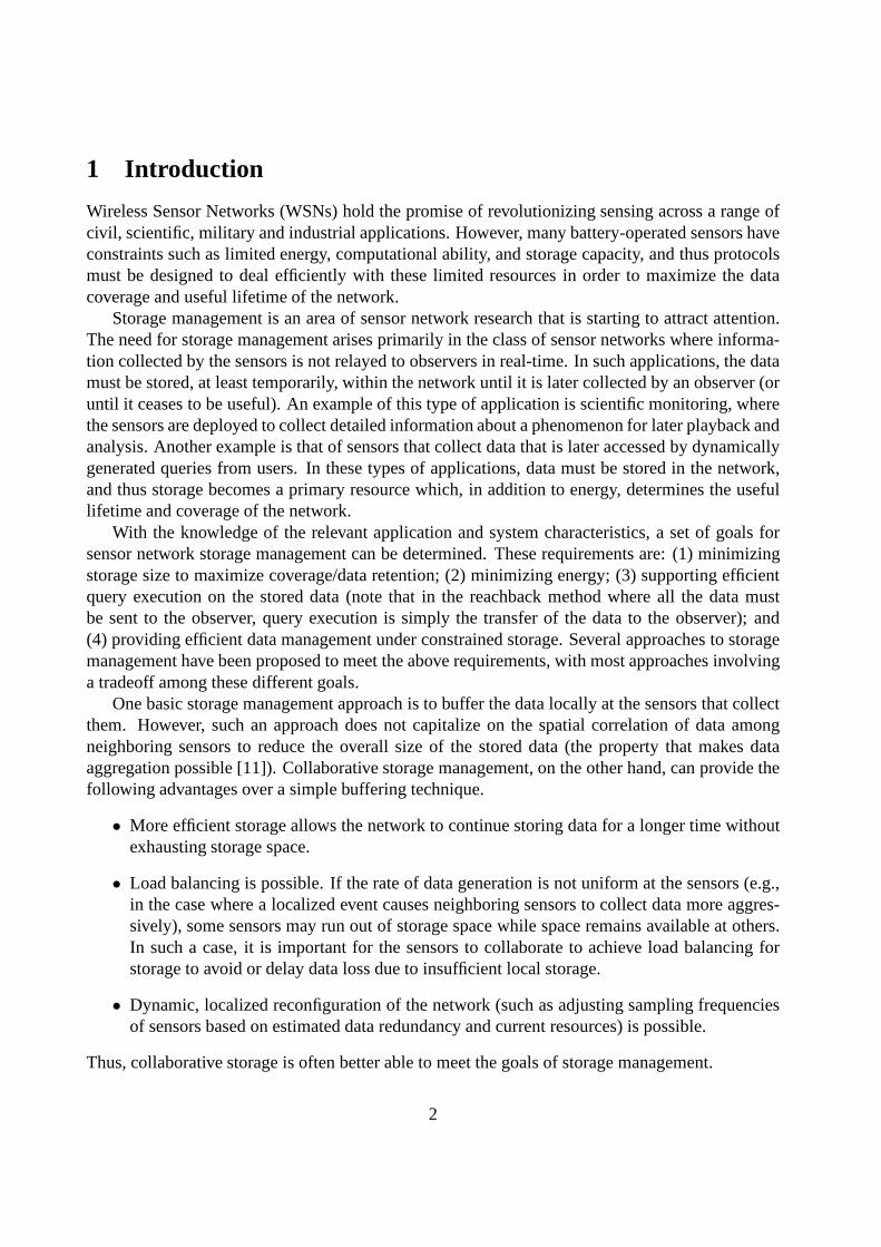
Figure 1(a) shows the average storage used per sensor as a function of the number of sensors (50,100 and 150 sensors) for the four storage management techniques : (1) local storage (LS); (2)Cluster-Based Collaborative Storage (CBCS); (3) Coordinated Local Storage (CLS); and (4) Co-ordinated Collaborative Storage (CCS). In the case of CBCS,the aggregation ratio was set to 0.5.The storage space consumption is independent of the networkdensity for LS and is greater thanthe storage space consumption for CBCS and CCS (roughly in proportion to the aggregation ratio).CLS storage requirement is in between the two approaches because it is able to reduce the stor-age requirement using coordination (we assumed that coordination yields improvement uniformlydistributed between 20% and 40%). Note that after data exchange, the storage requirement forCBCS and CCS are roughly the same since aggregation at the cluster head can reduce the data toa minimum size, regardless of whether coordination took place or not.

11

50 100 1500

0.5

1

1.5

2

2.5

3

3.5

4

4.5

5x 10

5

Number of Sensors

Mea

n S

tora

ge S

pace

Con

sum

ed (

Byt

es)

Storage space as a function of Network SizeLocal−BufferCLSCBCSCCS

(a) Storage space vs. Network Density

L−1 CLS−1 C−1 CCS−1 L−2 CLS−2 C−2 CCS−2 L−3 CLS−3 C−3 CCS−30

0.1

0.2

0.3

0.4

0.5

0.6

0.7

0.8

0.9

Number of SensorsM

ean

Ene

rgy

(J)

Energy Consumption study as a function of Network Size

Pre−EnergyPost−Energy

(b) Energy consumption vs. NetworkDensity

Figure 1: Comparison between local storage (LS), cluster based collaborative storage (CBCS),coordinated local storage (CLS) and coordinated collaborative storage (CCS).

Surprisingly, in the case of collaborative storage, the storage space consumption decreasesslightly as the density increases. While this is counter-intuitive, it is due to the higher packet lossobserved during the exchange phase as the density increases; as density increases, the probabilityof collisions increases. These losses are due to the use of a contention based unreliable MAC layerprotocol. The negligible difference in the storage space consumption between CBCS and CCS isalso an artifact of the slight difference in the number of collisions observed in the two protocols.A reliable MAC protocol such as that in IEEE 802.11 (which uses four-way handshaking) or areservation based protocol such as the TDMA based protocol employed by LEACH [9] can be usedto reduce or eliminate losses due to collisions (at an increased communication cost). Regardless ofthe effect of collisions, one can clearly see that collaborative storage achieves significant savingsin storage space compared to local storage protocols (in proportion to the aggregation ratio).

We assumed Transfer Energy/MB0.055J for flash memory. In the case of ratio, we assumedTransmit Power= 0.0552W , Receive Power= 0.0591W , and Idle Power= 0.00006W . Fig-ure 1(b) shows the consumed energy for the protocols in Joules as a function of network density.

The X-axis represents protocols for different network densities: L and C stand for local buffer-ing and CBCS respectively. L-1,L-2,and L-3 represent the results using the local buffering tech-nique for network size 50, 100 and 150, respectively. The energy bars are broken into two parts:pre-energy, which is the energy consumed during the storagephase, and post-energy, which is theenergy consumed during data collection (the relaying of thedata to the observer). The energyconsumed during the storage phase is higher for collaborative storage because of the data com-munication among neighboring nodes (not present in local storage) and due to the overhead forcluster rotation. CCS spends less energy than CBCS due to thereduction in data size that resultsfrom coordination. However, CLS has higher expenditure than LS since it requires costly commu-nication for coordination. This cost grows with the densityof the network because our coordinationimplementation has each node broadcasting its update and receiving updates from all other nodes.

12

1 2 3 4 5 6 7 8 90

10

20

30

40

50

60

70

80

90

100

Time (in multiple of 100 seconds)

Per

cent

age

of S

enso

rs w

ithou

t Sto

rage

Percentage of Storage Depleted Sensors versus time

Local−EvenCollaborative−EvenLocal−UnevenCollaborative−Uneven

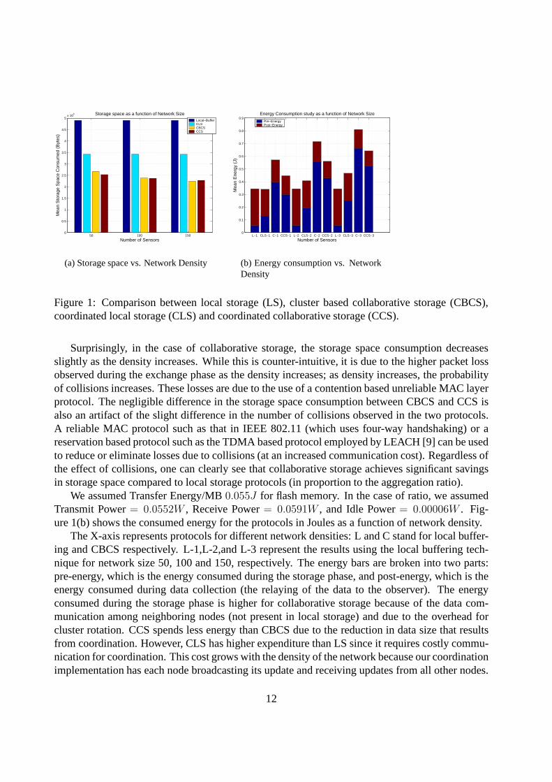
Figure 2: Percentage of storage depleted sensors as a function of time.

For the storage and communication technologies used, the cost of communication dominatesthat of storage. As a result, the cost of the additional communication during collaborative storagemight not be recovered by the reduced energy needed for storage except at very high compressionratios. This tradeoff is a function of the ratio of communication cost to storage cost; if this ratiogoes down in the future (for example, due to the use of infra-red communication or ultra-lowpower RF radios), collaborative storage becomes more energy efficient compared to local storage.Conversely, if the ratio goes up, collaborative storage becomes less efficient.

5.4.2 Storage Balancing Effect

In this study, we explore the load-balancing effect of collaborative storage. More specifically,the sensors are started with a limited storage space, and thetime until this space is exhausted istracked. We consider an application where a subset of the sensors generates data at twice the rateof the others, for example, in response to higher observed activity close to some of the sensors. Tomodel the data correlation, we assume that sensors within a zone have correlated data. Therefore allthe sensors within a zone will report their readings with thesame frequency. We randomly selectzones with high activity; sensors within those zones will report twice as often as those sensorswithin low activity zones.

In Figure 2, the X-axis denotes time (in multiples of 100 seconds), whereas the Y-axis denotesthe percentage of sensors that have no storage space left. Using LS, in the even data generationcase, all sensors run out of storage space at the same time andall data collected after that is lost.In comparison, CBCS provides longer time without running out of storage because of its moreefficient storage.

The uneven data generation case highlights the load-balancing capability of CBCS. Using LS,the sensors that generate data at a high rate exhaust their storage quickly; we observe two sub-sets of sensors getting their storage exhausted at two different times. In comparison, CBCS hasmuch longer mean sensor storage depletion time due to its load balancing properties, with sensorsexhausting their resources gradually, extending the network lifetime much longer than LS.

The sensor network coverage from a storage management perspective depends on the event

13

generate rate, the aggregation properties and the available storage. If the aggregated data size isindependent of the number of sensors (or grows slowly with it), the density of the zone correlateswith the availability of storage resources. Thus, both the availability of storage resources as wellas the consumption of them may vary within a sensor network. This argues for the need of load-balancing across zones to provide long network lifetime andeffective coverage. This is a topic offuture research.

Collaborative storage reduces storage requirements by taking advantage of temporal and spatialcorrelations in data from nearby sensors. Furthermore, coordinated storage proactively exploitsspatial redundancy in sensor data, thereby reducing not only storage requirements but also energydissipation in communication of the data as well as in the sensing hardware, which can be turnedoff on nodes that are not assigned to sense data for the current period. Another approach that takesadvantage of the correlations in the data to manage storage space is the multi-resolution technique,described next.

5.5 Multi-Resolution Based Storage

Much existing research, such as Directed Diffusion [12], Data Centric Storage (DCS) [21], TAG [16],Cougar [2], etc. has focused on in network aggregation and query processing when features of in-terest are known. For example, DCS stores named events at known locations to reduce queryoverhead. Since the events are constellations of low-levelsensor observations, they are not storageintensive. Therefore DCS does not address the issue of managing limited storage space. TAGassumes knowledge of aggregation operators. Recently, Ganesan et al. [4]proposed an in-networkwavelet-based summarization technique accompanied by progressive aging of these summariesto support data-intensive applications where features of interest are not known in advance andthe networks are storage and communication-constrained. Their system strives to support storageand search for raw sensor data (low-level observations) in data-intensive scientific applications byproviding a lossy, progressively degrading storage model.The key factors of this work are wavelet-based spatio-temporal data summarization (construction of multi-resolution summaries of data), ahierarchically decomposed distributed storage structure, drill-down queries, and progressive agingof summaries. We briefly describe each of these features in detail in next few sections.

5.5.1 Multi-Resolution Summarization

The authors proposed the use of a wavelet based data summarization technique that is carried outin two steps, namely temporal and spatial summarization.

Temporal summarization is done by every sensor node locallyusing techniques such as time se-ries analysis to find redundancy in its own signal. Temporal summarization involves just computation—no communication is needed.

Spatial summarization involves constructing a hierarchy and using spatio-temporal summariza-tion techniques to re-summarize data at each level. Also, data at lower levels can be summarizedat higher levels at larger spatial scale but with higher compression (thereby it is more lossy).

14

5.5.2 Drill Down Queries

The basic idea behind drill-down queries is quite intuitive. Data are summarized at multiple res-olutions across the network. Queries are injected at the highest level of hierarchy, which has thecoarsest and most highly compressed summary of very large spatio-temporal data. Processing thequery over this summary gives an approximate answer/pointer to the part of the network that isvery likely to give a more accurate answer, since it has a moredetailed view of the subregion. Fur-ther queries can then be directed to this region, if needed. This process is applied recursively untilthe user is satisfied with the accuracy of the result or the leaves of the hierarchy are encountered.Clearly, the accuracy of the result (query quality) improves with more drill-downs since finer datagets queried at lower levels.

Hierarchical summarization and drill down query together address the challenges in searchingdata in an efficient manner. After describing how to compute the summaries, we now discussanother challenging issue that deals with storage space allocation/reclaim of these summaries in adistributed fashion.

5.5.3 Aging Problem

In storage-constrained networks, a challenging question is to decide how long a summary is to bestored. The length of time for which a summary is stored is called anageof the summary. Letf(t) be a monotonically decreasing user-specified aging function that represents the error the useris willing to accept as the data ages in the network. The authors argue that, typically the domainexperts can supply this kind of function. As an example, the user might be willing to accept 90%query accuracy for data that is a week old data but only 50% accuracy for data that is a year old.Let us denote the instantaneous quality difference asqdiff(t), which represents the user-specifiedaging function and the achieved query accuracy at give timet. The aging problem can be definedas follows. Find the ages of summaries,Agei, at different resolutions such that the maximuminstantaneous quality difference is minimized.

Min0≤t≤T (Max(qdiff(t))) (1)

under the constraints:

• Drill Down Constraints: It is not useful to retain a summary at lower levels if its summary athigher levels is not present, since drill down queries will not be directed to the lower levelsin that case.

• Storage Constraints: Each node has a finite storage space available to the summaries of eachlevel.

The authors proposed three aging strategies, namely omniscient, training-based and greedystrategy, and evaluated their performance.

15

6 Indexing and Data Retrieval

The final challenge that we discuss in storage management is indexing and retrieval of the data.In the case of the first application type (Scientific Monitoring/Partitioning), the data is relayedback to an observer during reach-back one time. Accordingly, indexing and retrieval is not animportant issue for this type of application. Nevertheless, reducing storage size leads to moreefficient retrieval in terms of time and energy. Furthermore, it is possible to improve the retrievalperformance if the expected location of the observer is known by favoring sensors closer to theobserver.

Indexing and retrieval are more important issues in our second application model (Augmentedreality), where data can be queried dynamically and by multiple observers. Such networks areinherently data-centric; observers often name data in terms of attributes or content that may not betopologically relevant. For example, a commander may be interested in enemy tank movements.This characteristic of sensor networks is similar to many peer-to-peer (P2P) environments [1]which are also often data-centric. Such a model is in contrast with traditional host-centric ap-plications such as telnet, where the end user is communicating with a specific end-host at the otherend. We first overview peer-to-peer solutions to data indexing and retrieval and then show that theproperties of sensor networks significantly change the tradeoffs and invite different solutions.

6.1 Design Space – Retrieval in P2P Networks

In P2P networks, the problem of data indexing and retrieval has been attacked in several ways.These approaches can be classified in terms of data placementas: (1) structured: the data is placedat specific locations (e.g., using hashing on keys) to make retrieval more efficient [25, 20]. Usingthis approach, a node that is searching for data can use this structure to figure out where to lookfor the data. However, this structure requires extensive communication of data and may not besuitable for sensor networks. Further, related data may be stored at many different locations,making queries inefficient; (2) unstructured: the data is not forced to specific locations [23]. Inthis case, searching for data is difficult since it may exist anywhere; in the worst case the user mustperform a random search. Replication improves the performance of retrieval [3], but is likely to betoo expensive for a sensor network environment.

For unstructured networks, P2P solutions differ in terms ofthe indexing support. Decentralizednetworks provide no indexing. Centralized networks provide a centralized index structure. Finally,hybrid centralized networks provide hierarchical indexing, where supernodes each keep track ofthe data present at the nodes managed by them.

While the tradeoffs between these approaches are well studied in the P2P community, it is notclear how they apply for sensor networks. Specifically, P2P networks exist on the internet whereresources are not nearly as limited as those in a sensor network. Solutions requiring large datamovement or expensive indexing are likely to be inefficient.It is also unclear what keys/attributesshould be indexed to facilitate execution of common queries. Finally, solutions that cause ex-pensive query floods will also be inefficient. In the remainder of this section, we study existingresearch into indexing and retrieval in sensor networks.

16

Table 2: Comparison of different canonical methods.Method Total HostspotExternal Storage Dtotal

√n Dtotal

Local Storage Qn + Dq

√n Q + Dq

Data-Centric (Summary) Q√

n + Dtotal

√n + Q

√n 2Q

6.2 Data Centric Storage – Geographic Hash Tables

In the context of peer-to-peer systems, Distributed Hash Tables (DHTs) are a decentralized struc-tured P2P implementation. Typically these DHTs provide thefollowing simple yet powerful inter-face: Put(datad,keyk) operation, which stores the given data itemd based on its keyk. Get(keyk) operation can be used to retrieve all the data items matching the given keyk.

The Geographic Hash Table (GHT) system implements a structured P2P solution for data cen-tric storage (DCS) in sensor networks [21]. Even though GHT provides an equivalent functionalityto structured P2P systems, it needs to address several new challenges. Specifically, moving data iscostly in sensor networks. Moreover, the authors target keeping related data close such that queriescan be more focused and efficient.

In the next few sections we describe how GHT incorporates physical connectivity in data-centric operations in resource-constrained sensor networks. Before delving into the details ofGHT based data centric storage, we overview three canonicaldata dissemination methods alongwith their approximate communication costs and demonstrate the usefulness of data-centric stor-age [21].

6.2.1 Canonical Methods

The primary objective of a data dissemination method is to extract relevant data from a sensornetwork in an efficient manner. The following are three fundamentally different approaches toachieve this objective. Let us assume that the sensor network hasn nodes.

1. External Storage (ES): Upon detecting an event, the relevant data is sent to the base station.ES entailsO(

√n) cost for each event to get to the base station, with zero cost for queries

generated at the base station (external) andO(√

n) for queries generated within the sensornetwork (internal).

2. Local Storage (LS): In this case, a sensor node, upon detecting an event, stores the informa-tion locally. LS incursO(n) cost for query dissemination, since a query must be flooded andO(

√n) cost to report the event.

3. Data-Centric Storage (DCS): DCS stores named data withinthe network. It requiresO(√

n)cost to store the event and both querying and event response requireO(

√n) cost.

Let us assume that a sensor network detectsT event types, and denote the total number of eventsdetected byDtotal. Q denotes the number of event types queries andDQ denotes the number of

17

events detected for each event queried. Further, assume that there are a total ofQ queries (oneper event type). Table 6.2.1 shows the approximate communication cost for the three canonicalmethods. Total cost accounts for the total number of packetssent in the network, whereas thehostspot usage denotes the maximum number of packets sent byany particular sensor node.

¿From this analysis, its clear that no single method is preferable under all circumstances. Ifthe events are accessed more frequently than they are generated (by external observers), externalstorage might be a good alternative. On the other hand, localstorage is an attractive option whenthe events are generated more frequently and accessed infrequently. DCS lies in the middle ofthese two options and is preferable in cases where the network is large and a large number ofevents are detected but few are queried. The next sections provide the implementation details anda discussion of GHT.

6.3 GHT: A Geographic Hash Table

GHT is a structured approach to sensor network storage that makes it possible to index data basedon content without requiring query flooding. GHT also provides load-balancing of storage usage(assuming fairly uniform sensor deployment). GHT implements a Distributed Hash Table by hash-ing a keyk into geographic coordinates. As mentioned above, GHT supports Put(datad,key k)and Get(keyk) operations in the following way. In Put, data (events) are randomly hashed to ageographic location (x, y coordinates), whereas a Get operation on the same keyk hashes to thesame location. In the case of sensor networks, sensors can bedeployed randomly and the geo-graphic hashing function is oblivious to the topology. Therefore it might happen that a sensor nodemight not exist at the precise location given by the hash function. Also, it is crucial to ensureconsistency between Get and Put operations, i.e., both of them map the same key to the same node.Put achieves that by storing the hashed event at the nodenearestto the hashed location and Getoperations can also retrieve an event from the nodenearestto the hashed location. Of course, thispolicy ensures the desired consistency between Get and Put operations.

GHT uses Greedy Perimeter Stateless Routing (GPSR) [14]. GPSR is a geographic routingprotocol that just uses location information to route packets to any connected destination. It as-sumes that every node knows its own location and also locations of its all one-hop neighbors. Ithas two flavors of routing algorithms: greedy forwarding andperimeter forwarding.

In the case of greedy forwarding, a node X upon receiving a packet for a destination D, forwardsit to its neighbor that is closest to D among all its neighborsincluding X itself. Intuitively, a packetmoves closer to the destination each time it gets forwarded and eventually it reaches the destination.Of course, greedy forwarding does not work in the case when X does not have any neighbor closerto D than itself. GPSR then switches to its perimeter mode.

In the perimeter mode, GPRS uses the following right-hand rule: upon arriving on an edgeat node X, the packet is forwarded on the next edge counterclockwise about X from the ingressdegree. GPSR first computes a planar subgraph of the network connectivity graph and then appliesthe right hand rule to this graph.

18

6.3.1 Interaction of GHT with GPSR

GPSR provides the capability to deliver packets to a destination node located at the specified coor-dinates, whereas GHT requires the ability to forward a packet to a node closest to the destinationnode. GHT defines ahome nodeas the node that is closest to the hashed location; GHT requiresan ability to store an event at the Home node.

Let us assume that hashing an event gives location(X1, Y1) as the coordinates of the nodewhere the given event needs to be stored. Further let us assume that no node exists at location(X1, Y1). Then GHT would store that event at its Home Node H. So node H, upon receiving apacket for destination(X1, Y1), will switch to GPRS’s perimeter routing mode (since it willhaveno neighbor closer to the destination than itself). By applying perimeter routing, the packet willeventually return to H upon traversing the entire perimeter. H can then conclude that it is theHome node for the given event and then will store the event. The interaction between GHT andGPSR described so far works well for static sensors, ideal radios and without considering failuresof sensor nodes. However, when thousands of sensors are thrown in a hostile environment, one canhardly assume the presence of these ideal conditions.

GHT ensures robustness (resilience to node failure and topology changes) and scalability (bybalancing load across the network) as follows. It uses a novel perimeter refresh protocol to achieverobustness in the face of node failures and topology changes, and it uses structured replication todo load balancing, thereby achieving scalability. We now briefly describe these two techniques.

6.3.2 Perimeter Refresh Protocol

GHT needs to address two challenges, namely home node failure and topology changes (e.g.,addition of nodes). Periodically, a home node initiates a perimeter refresh message that traversesacross the entire perimeter of the specified location. Everynode on the perimeter, upon receivingthis event, first stores it locally and then marks the association between the given event and thehome node for a certain duration with the help of a timer. If the node receives any subsequentrefresh messages from the same home node, it resets the timerand reassociates the home nodewith the event. However, if it fails to receive the refresh message, it assumes that the home nodefor the event has failed and initiates a refresh message on its own for electing a new home node. Inthis manner, GHT recovers from home node failures.

Due to topology changes, it might happen that some new nodeH1 is now closer to the destina-tion than the current home nodeH. When the current home nodeH initiates the refresh message,H1 will receive it. SinceH1 is closer to the destination thanH (by definition of the home node), itreinitiates the refresh message which then passes through all the nodes on the perimeter includingH and eventually returning toH1. All the nodes on the perimeter update their associations andtimers accordingly to point toH1. In this way, GHT addresses the issue of topological changes.

6.3.3 Structured Replication

If many events are hashed onto same node (location) then thisnode can become ahot-spot. Struc-tured replication is GHT’s way to balance the load and reducethe hot-spot effect. The basic idea

19

is to decompose the hierarchy geographically and replicatethe home node rather then replicatingthe data itself. For example, instead of storing data at the root of the hierarchy (home node of theevent), a node stores the data at the nearest mirror node (oneof the replicas of the home node).For retrieving events, queries are still targeted towards the root node; however, the root node thenforwards the query to the mirror node.

6.4 Graph EMbedding for Sensor Networks (GEM)

GHT uses GPSR, a geographic routing protocol that routes packets just based on location informa-tion. GEM (Graph EMbedding for sensor networks) is an infrastructure for node-to-node routingand data-centric storage and information processing in sensor networks without using geographicinformation [18]. GEM embeds a ringed tree into the network topology and labels nodes in a wayto construct a VPCS (Virtual Polar Coordinate Space). VPCR is a routing algorithm that runs ontop of VPCS and requires no geographic information. It provides the ability to create consistentassociations without relying on geographic information.

6.5 Distributed Index for Features in Sensor Networks (DIFS)

GHT targets retrieval of high-level, precisely defined events. The original GHT implementation islimited to report whether a specific high-level event occurred. However, it is not able to efficientlylocate data in response to more complex queries. The Distributed Index for Features in SensorNetworks (DIFS) attempts to extend the original architecture to efficiently support range queries.Range queries are the queries where only events within a certain range are desired. In DIFS, theauthors propose a distributed index that provides low average search and storage communicationrequirements while balancing the load across the participating nodes [8]. We now describe thenotion of high-level events and discuss a few sample range queries that can be posed by the enduser.

6.5.1 High-level Event

A High-level event can be defined in terms of composite measurements of sensor values them-selves. For example, a user might query average animal speed, peak temperature in hot regions,etc. Often the user can add timing constraints to these values: for example, a user may query theaverage animal speed within the last hour. Alternatively, the user might incorporate a spatial di-mension as well: for example, a user may look for an area with average temperature greater than acertain threshold. Some end users might be interested in querying relations among various eventsas well. An example of a query in the temporal domain: Is an increase in temperature above athreshold followed by the detection of an elephant? Of course, all the above types can be used incombination, and more complex queries can be posed. DIFS assumes that all sensors store rawsensor readings, while only a subset of sensors serve as an index node to facilitate the search. Notethat DIFS runs on top of GHT to support the above mentioned range queries in an efficient way.Since the reader is already familiar with GHT, we first describe a naive quad tree based approachfor indexing followed by the DIFS architecture.

20

6.5.2 Simple Quad Tree Approach

This approach works by constructing a spatially distributed quad tree of histograms that summarizeactivity within the area they represent. A root node maintains four histograms describing thedistribution of data in each of four equi-sized quadrants (its children). A drill down-query approachcan be used on top of this tree; the summaries at children nodes are more detailed. However, inthat case, since the root node has to process all the queries (queries move in top-down fashion overthe tree), it might prove to be a bottleneck. Also, propagating data up in the hierarchy to updatehistograms every time a new event gets generated might pose problems from an energy point ofview. DIFS extends this naive approach to address these problems.

6.5.3 DIFS architecture

Similar to the quad tree implementation, DIFS constructs anindex hierarchy using histograms.Unlike the quad tree approach, every child hasbfactnumber of parents instead of a single parent,wherebfact = 2i, i ≥ 1. Also, the range of values a child maintains in its histograms is bfacttimes the range of values maintained by its parent. The crucial point is that, to ensure energy-storage load balancing, a range of values an index node knowsabout is inversely proportional tothe spatial extent it covers. Therefore, rather than havingonly one query entry point,as in the caseof naive quad tree approach, a search may begin at any node in the tree. Query entry points areselected according to both the spatial extent, as well as therange of values mentioned in the query.

Another important feature isindex node selection. Index node selection is done with the helpof a geographically bound hash function. A given sensor fieldis divided into rectangular quadrantsrecursively proportional to the number of levels in the index hierarchy. Given a source location, astring to hash, and a bounding box, the output of this hash function is a pair of coordinates withinthe given bounding box. Note that, in the case of GHT, the hashfunction can result to any locationwithin the sensor field and not to any location within the bounding box. Intuitively, a node forwardsan event to the first local index node with the narrowest spatial coverage but widest value range.This node then forwards it to its parent with wider spatial coverage but narrower value range. Thisforwarding process can be applied recursively.

7 Concluding Remarks

In this chapter, we considered the problem of storage management for sensor networks wheredata are stored in the network. We discussed two classes of applications where such storage isneeded: (1) Off-line scientific monitoring: data is collected off-line and periodically gathered byan observer for later playback and analysis; and (2) Augmented reality applications: data is storedin the network and used to answer dynamically generated queries from multiple observers. In suchstorage-bound networks, the sensors are limited not only interms of available energy, but also interms of storage. Furthermore, efficient data-centric indexing and retrieval of the data is desirable,especially for the second application type.

We have identified the goals, challenges and design considerations present in storage-boundsensor networks. We organized the challenges into three areas, each incorporating a unique de-

21

sign/tradeoff space with respect to the identified goals. Moreover, each of the areas has preliminaryexisting research and protocols. These areas are:

1. System support for storage: storage for sensors is different from traditional non-volatilestorage both in terms of the hardware, applications and resource limitations. As such, thehardware and required file system support differ significantly from traditional systems.

2. Collaborative storage: storage can be minimized by exploiting spatial correlation betweennearby sensors and by reducing redundancy/adjusting sampling periods. Such techniquesrequire data exchange among nearby sensors (and the associated energy costs). An intricatetradeoff in terms of energy exists: local buffering may saveenergy during the data collectionphase but not during indexing and data retrieval. Furthermore, storage and energy may needto be balanced depending on the resource that is scarcer.

3. Indexing and retrieval: the final problem is similar to theindexing and retrieval problem inP2P networks. However, it differs in the type of data and the high costs for communica-tion (requiring optimized queries and limiting of unnecessary data motion). We discussedexisting solutions in this area.

Most existing work addresses these different aspects of theproblem independent of the others.We believe that there remains large areas of the design spacein each area that are unexplored.However, issues at the intersection of these areas appear most challenging and have not been ad-dressed to our knowledge.

References

[1] S. Androutsellis-Theotokis. A survey of peer-to-peer file sharing technologies, 2002. Avail-able on the Web: http://www.eltrun.aueb.gr/whitepapers/p2p_2002.pdf .

[2] P. Bonnet, J. Gehrke, and P. Seshadri. Towards sensor database systems.Lecture Notes inComputer Science, 1987, 2001.

[3] E. Cohen and S. Shenker. Replication strategies in unstructured peer-to-peer networks. 2002.in The ACM SIGCOMM’02 Conference, August 2002.

[4] D. Ganesan, B. Greenstein, D. Perelyubskiy, D. Estrin, and J. Heidemann. An evaluationof multi-resolution storage for sensor networks. InProceedings of the first internationalconference on Embedded networked sensor systems, pages 89–102. ACM Press, 2003.

[5] D. Ganesan, S. Ratnasamy, H. Wang, and D. Estrin. Coping with irregular spatio-temporalsampling in sensor networks.ACM Computer Communication Review (CCR), 2004. (forth-coming).

[6] D. Gay. Design of matchbox, the simple filing system for motes, 2003. Available on the Web:http://www.tinyos.net/tinyos-1.x/doc/matchbox.pdf .

22

[7] D. Gay. Matchbox: A simple filing system for motes, 2003. Available on the Web:www.tinyos.net/tinyos-1.x/doc/matchbox-design.pdf .

[8] B. Greenstein, D. Estrin, R. Govindan, S. Ratnasamy, andS. Shenker. Difs: A distributed in-dex for features in sensor networks. InFirst IEEE International Workshop on Sensor NetworkProtocols an Applications (SNPA 2003), 2003.

[9] W. Heinzelman. Application-Specific Protocol Architectures for WirelessNetworks. PhDthesis, Massachusetts Institute of Technology, 2000.

[10] J. Hill, R. Szewczyk, A. Woo, S. Hollar, D. E. Culler, andK. S. J. Pister. System architecturedirections for networked sensors. InArchitectural Support for Programming Languages andOperating Systems, pages 93–104, 2000.

[11] C. Intanagonwiwat, D. Estrin, R. Govindan, and J. Heidemann. Impact of network density ondata aggregation in wireless sensor networks. Technical Report TR-01-750, Univ. of SouthernCalifornia, Nov. 2001.

[12] C. Intanagonwiwat, R. Govindan, and D. Estrin. Directed diffusion: A scalable and robustcommunication paradigm for sensor networks. InProc. 6th ACM International Conferenceon Mobile Computing and Networking (Mobicom’00), Aug. 2000.

[13] P. Juang, H. Oki, Y. Wang, M. Martonosi, L. S. Peh, and D. Rubenstein. Energy-efficientcomputing for wildlife tracking: design tradeoffs and early experiences with zebranet. InProceedings of the 10th international conference on architectural support for programminglanguages and operating systems, pages 96–107. ACM Press, 2002.

[14] B. Karp and H. T. Kung. Gpsr: greedy perimeter statelessrouting for wireless networks. InProceedings of the 6th annual international conference on Mobile computing and networking,pages 243–254. ACM Press, 2000.

[15] S. Madden.The Design and Evaluation of a Query Processing Architecture for Sensor Net-works. PhD thesis, U.C. Berkeley, 2003.

[16] S. Madden, M. Franklin, J. Hellerstein, and W. Hong. Tag: a tiny aggregation service forad-hoc sensor networks. InOSDI, 2002.

[17] M. K. McKusick, W. N. Joy, S. J. Leffler, and R. S. Fabry. A fast file system for UNIX.Computer Systems, 2(3):181–197, 1984.

[18] J. Newsome and D. Song. Gem: Graph embedding for routingand data-centric storage in sen-sor networks without geographic information. InProceedings of the First ACM Conferenceon Embedded Networked Sensor Systems (SenSys 2003)., 2003.

[19] Network Simulator. http://isi.edu/nsnam/ns.

23

[20] S. Ratnasamy, P. Francis, M. Handley, R. Karp, and S. Shenker. A scalable content address-able network. InProceedings of ACM SIGCOMM 2001, 2001.

[21] S. Ratnasamy, B. Karp, S. Shenker, D. Estrin, R. Govindan, L. Yin, and F. Yu. Data-centricstorage in sensornets with ght, a geographic hash table.Mob. Netw. Appl., 8(4):427–442,2003.

[22] A remote ecological micro-sensor network, 2000. (Available on the web at:http://www.botany.hawaii.edu/pods/overview.htm ).

[23] M. Ripeanu, I. Foster, and A. Iamnitchi. Mapping the gnutella network: Properties of large-scale peer-to-peer systems and implications for system design. IEEE Internet ComputingJournal, 6(1).

[24] M. Rosenblum and J. K. Ousterhout. The design and implementation of a log-structured filesystem.ACM Transactions on Computer Systems, 10(1):26–52, 1992.

[25] I. Stoica, R. Morris, D. Liben-Nowell, D. R. Karger, M. F. Kaashoek, F. Dabek, andH. Balakrishnan. Chord: a scalable peer-to-peer lookup protocol for internet applications.IEEE/ACM Trans. Netw., 11(1):17–32, 2003.

[26] S. Tilak, N. Abu-Ghazaleh, and W. Heinzelman. Storage management issues forsensor networks. Available on the Web:www.cs.binghamton.edu/˜sameer/CS-TR-04-NA01 .

[27] Crossbow Technology Inc. http://www.xbow.com.

24