Storage and balancing synergies in a fully or highlyrenewable pan-European power system

Morten Grud Rasmussena,b,1, Gorm Bruun Andresenb,2, Martin Greinerb

aCenter for Mathematical Sciences and Institute for Advanced Study, TechnischeUniversitat Munchen, 85748 Garching, Germany

bDepartment of Engineering and Department of Mathematics, Aarhus University, NyMunkegade 118, 8000 Aarhus C, Denmark

Abstract

Through a parametric time-series analysis of eight years of hourly data, we

quantify the storage size and balancing energy needs for highly and fully re-

newable European power systems for different levels and mixes of wind and

solar energy. By applying a dispatch strategy that minimizes the balancing en-

ergy needs for a given storage size, the interplay between storage and balancing

is quantified, providing a hard upper limit on their synergy. An efficient but

relatively small storage reduces balancing energy needs significantly due to its

influence on intra-day mismatches. Furthermore, we show that combined with

a low-efficiency hydrogen storage and a level of balancing equal to what is to-

day provided by storage lakes, it is sufficient to meet the European electricity

demand in a fully renewable power system where the average power generation

from combined wind and solar exceeds the demand by only a few percent.

Keywords: energy system design, wind power generation, solar power

generation, large-scale integration, storage

1. Introduction

A fully renewable pan-European power system will depend on a large share

of non-dispatchable, weather dependent sources, primarily wind and solar power

Email address: mgr@imf.au.dk (Morten Grud Rasmussen)1This author is supported by Carlsbergfondet2This author is supported by DONG Energy

Preprint submitted to Elsevier August 31, 2012

(Czisch (2005); Jacobson and Delucchi (2011)). The optimal ratio between and

necessary amount of wind and solar power depends on storage and balancing re-

sources (Heide et al. (2010, 2011); Hedegaard and Meibom (2012)), transmission

(Czisch and Giebel (2007); Kempton et al. (2010); Schaber et al. (2012a,b)), and

the characteristics of the climate (Widen (2011); Aboumahboub et al. (2010))

and load (Yao and Steemers (2005)). Based on meteorological data, it was shown

that even with unlimited transmission within Europe, a scenario with only wind

and solar power in combination with either only storage (Heide et al. (2010)) or

only balancing (Heide et al. (2011)) requires a very large amount of excess gen-

eration in order to be technically feasible. Here, we study the intermediate and

more realistic scenarios where power generation from the two weather-driven

variable renewable energy (VRE) sources is backed up by specific combinations

of storage and balancing. We identify a class of realistic and feasible scenarios

for building a fully or partially renewable pan-European power system.

The main point of our paper is to outline what is possible in a wind and solar

based European power system with storage and balancing systems. The power

capacities of the storage and balancing facilities are not determined; this would

require a more complex modeling with explicit inclusion of power transmission

(Rodriguez et al. (2012)). We focus on wind and solar power and assume no

bottlenecks in the power grid, employ an optimal storage dispatch strategy

and ignore storage charge and discharge capacities and economic aspects. The

incentives for doing so are closely related and at least threefold.

By assuming few technical constraints and optimal operation strategy, our

results provide a hard upper limit on what can be accomplished by better in-

tercontinental power network integration, better technology or better market

design. This means that more realistic models have a solid frame of refer-

ence to be measured up against. At the same time, our results provide precise

boundaries for policy makers. Furthermore, it allows for a simpler analysis and

a clearer presentation. The price is that a more detailed model is necessary

2

in order to give useful answers to questions regarding e.g. charge, discharge3,

balancing or power flow capacities, and hence any considerations regarding the

economic costs obviously become highly speculative within the current modeling

framework.

A somewhat related but in some respects also parallel argument is behind the

decision of focusing on wind and solar power. Three of the most scalable renew-

able energy sources are wind and solar power and biomass. Of these, biomass

stands out as being dispatchable, meaning that it can be used for balancing

the intermittent (or non-dispatchable) power sources, such as wind and solar

power. As such, biomass is implicitly included in our analysis. Besides wind

and solar power, one of the most important non-dispatchable power sources is

run-of-river hydro power. Although run-of-river contributes significantly to the

present-day power systems of Europe with some percent of the total genera-

tion, the perspective for future growth is highly limited (Lehner et al. (2005)),

leaving it ill-suited as a third component in our parametric analysis. However,

with available data, it would have been straight-forward and an obvious choice

to include it as a fixed (but time dependent) contribution.

Contrary to most work done in this field (Czisch (2005); Jacobson and

Delucchi (2011); Martinot et al. (2007); Lund and Mathiesen (2009)), the novel

weather-based modeling approach, used here and first introduced in Heide et al.

(2010), is designed to investigate a whole class of scenarios. This means that

we do not only provide results for a few end-points, or for a pathway to any

such. Rather, we provide a continuous map of results for any combination and

penetration level of wind and solar power generation (Heide et al. (2010, 2011);

Schaber et al. (2012b)). We do not attempt to show that a transition to a

fully renewable power system is economically viable, however, this has been ad-

dressed by others (Czisch (2005); ECF (2010)). An advantage of disregarding

the economical aspect is that our work is less sensitive to technological advances

and socio-economic changes that could potentially shift the economic balance

3See, however, the Appendix

3

between e.g. wind and solar power.

The paper is organized as follows: Section 2 describes data and methodology.

Section 3 briefly discusses the extreme scenarios of no storage and sufficiently

large storage, respectively. Section 4 deals with the interplay between storage

and balancing. Section 5 treats the concrete example of having a 6-hour storage.

Section 6 discusses the impact of hydro balancing and large hydrogen storages.

Finally, an appendix discusses storage operation strategies.

2. Data and methodology

2.1. Weather and load data

Historical weather data from the 8-year period 2000–2007 with a tempo-

spatial resolution of 1 hour × 50 × 50 km2 was used to derive wind and solar

power generation time series for Europe (see Heide et al. (2010)). The data set

comprise two 70128-hour long time series for each of the approximately 2600

grid cells, covering 27 European countries including off-shore regions. In this

study all grid cells are aggregated using a capacity layout based on political

goals and attractiveness of the sites (see Heide et al. (2010)). We thus have two

hourly power generation time series for Europe, w(t) for wind and s(t) for solar

power generation, where t denotes any hour of the 8-year period.

The electrical load time series L(t) is based on data from the transmission

system operators (TSO) for the same eight years. The load data was de-trended

to compensate for the approximately 2% yearly increase in demand and scaled

to 2007 values, where the total annual consumption amounted to 3240 TWh for

Europe. This corresponds to an average hourly load (av.h.l.) of 370 GWh.

The power generation time series w(t) and s(t) have been normalized to

the average electrical load, yielding two new time series, W (t) and S(t). As

everything is scaled to 2007 values, we use the units av.h.l. (average hourly

load) and av.y.l. (average yearly load) throughout the paper. This means that

W (t) =w(t)

〈w〉· av.h.l., S(t) =

s(t)

〈s〉· av.h.l.

4

and

〈L〉 = 〈W 〉 = 〈S〉 = 1 av.h.l.,

where 〈 · 〉 denotes the average value of a time series. In these units, the values of

L(t) all lie in the range 0.62–1.47 av.h.l. while W (t) and S(t) fall in the intervals

0.07–2.61 and 0.00–4.10 av.h.l., respectively. Figure 1 shows an excerpt of the

time series.

2.2. Generation–load mismatch

The generation–load mismatch time series ∆(t) is given by

∆(t) = γ · (αW ·W (t) + (1− αW ) · S(t))− L(t) , (1)

where αW denotes the wind power fraction of the average wind and solar power

generation and γ represents how much combined wind and solar power is gen-

erated on average, so that if e.g. γ = 1.00, the average total generation of wind

and solar power equals the average load. Using the standard notation

x− =

0 forx ≥ 0

−x forx < 0

, x+ =

x forx ≥ 0

0 forx < 0 ,

(2)

this means that ∆−(t) denotes the residual load, and ∆+(t) denotes possible

excess generation. We will use the term mix for any fixed choice of αW while γ is

referred to as the average VRE4 generation factor. An excerpt of the mismatch

time series ∆(t) for an average VRE generation factor γ = 1.00 and a mix of

αW = 0.60 together with the corresponding excerpt of the load and wind and

solar power time series can be seen in Figure 1.

2.3. Balancing

As our focus is on wind and solar based, fully renewable power systems, we

consider any dispatchable, additional power source to be balancing (excluding

4variable renewable energy

5

0123

[av.

h.l.]

Fri Sat Sun Mon Tue0.50.00.51.0

[av.

h.l.]

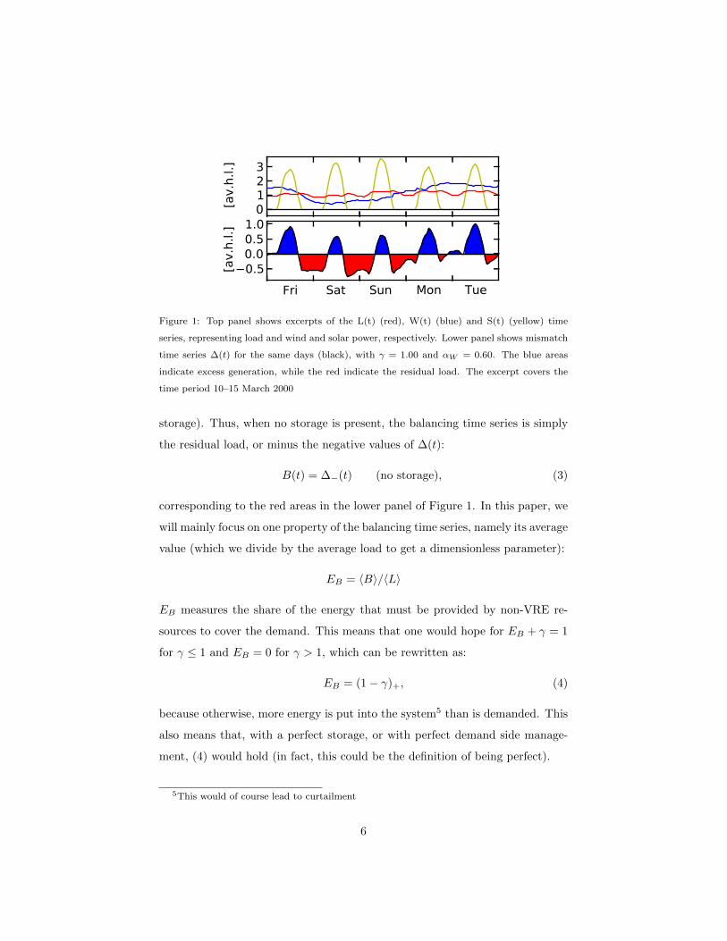
Figure 1: Top panel shows excerpts of the L(t) (red), W(t) (blue) and S(t) (yellow) time

series, representing load and wind and solar power, respectively. Lower panel shows mismatch

time series ∆(t) for the same days (black), with γ = 1.00 and αW = 0.60. The blue areas

indicate excess generation, while the red indicate the residual load. The excerpt covers the

time period 10–15 March 2000

storage). Thus, when no storage is present, the balancing time series is simply

the residual load, or minus the negative values of ∆(t):

B(t) = ∆−(t) (no storage), (3)

corresponding to the red areas in the lower panel of Figure 1. In this paper, we

will mainly focus on one property of the balancing time series, namely its average

value (which we divide by the average load to get a dimensionless parameter):

EB = 〈B〉/〈L〉

EB measures the share of the energy that must be provided by non-VRE re-

sources to cover the demand. This means that one would hope for EB + γ = 1

for γ ≤ 1 and EB = 0 for γ > 1, which can be rewritten as:

EB = (1− γ)+, (4)

because otherwise, more energy is put into the system5 than is demanded. This

also means that, with a perfect storage, or with perfect demand side manage-

ment, (4) would hold (in fact, this could be the definition of being perfect).

5This would of course lead to curtailment

6

Unfortunately, (4) cannot be expected to hold. This means that, for a given

γ, we could have EB > (1− γ)+, meaning that on average, we need additional

balancing. This leads us to define the additional average balancing EaddB as:

EaddB = EB − (1− γ)+ .

One can think of EaddB as a measure of how well the VRE resources can be

integrated into the power system, or how much energy one on average would

need to move in time to get perfect integration. We stress that EaddB is a property

that has to do with an average – it is not a priori possible to assign a time series

to the additional balancing. As one always – given γ – can find EB from EaddB

by adding (1− γ)+, and because EaddB makes some of the definitions related to

storages easier, we will mainly use EaddB rather than EB , except when we deal

with lossy storages, as the concept of additional balancing in this case becomes

more complicated.

2.4. Storage

With our goal of outlining the borders of what is possible in a European

power system with storage and balancing, in particular with respect to balancing

energy EB , we will focus on a storage dispatch strategy which, for a given storage

size CS , performs optimal with respect to EB . This means that given a storage

size, no storage dispatch strategy can result in a lower average balancing energy

EB than the one employed here. There are several strategies that satisfy this

condition, meaning that they all result in the same EB .

Here, we will present a version which has the advantages that it is simple and

hence easily defined and is easily seen to satisfy the condition, and it assumes

no foresight capabilities, but has the disadvantage that it is quite far from how

present-day real-world operation works. Three other versions satisfying the

minimum EB condition are presented in the appendix.

The version presented here can be summed up as a “storage first” strategy,

in the sense that any deficits are first covered with storage unless it runs empty,

and any excess generation is stored in the storage, unless the storage gets full.

7

No limits are imposed on the charge and discharge capacities. Conversion losses

in and out of the storage are modeled by storage efficiencies ηin and ηout. For

example, for hydrogen storage, the efficiencies are approximately 0.60 in both

directions (Beaudin et al. (2010); Kruse et al. (2002)), leading to a round-trip

efficiency of 0.36.

A storage is thus characterized by three parameters: ηin, ηout and CS . The

storage filling level time series H(t) with a constrained storage size CS is given

by:

H(t) =

CS for H(t− 1) + ∆(t) > CS ,

0 for H(t− 1) + ∆(t) < 0 ,

H(t− 1) + ∆(t) otherwise ,

(5)

where ∆ is given by the equation:

∆(t) = ηin∆+(t)− η−1out∆−(t) (6)

and H(tmin − 1) = H0 is an initial value to be determined, tmin being the first

hour of the time series. The storage works in the following way: Any excess

power at any time is fed into the storage with an efficiency of ηin, unless the

storage size is exceeded, in which case the storage is full. Any deficits in VRE

power generation as compared to the load are covered by the storage with an

efficiency of ηout, except if the storage runs empty, in which case the storage

only provides partial coverage of the deficit. The dispatch strategy is illustrated

in Figure 2.

To ensure storage neutrality, i.e. that the storage provides only as much

energy as is stored, we determine H0 in the following way: First, it is examined

whether the generation can match the demand. This is the case if ∆ sums up to

a non-negative value,∑

t ∆(t) ≥ 0 (equality is called equilibrium) or equivalently

ηinηout

∑t

∆+(t) ≥∑t

∆−(t) . (7)

If this is the case, we set the temporary variable H00 = CS , if not, H00 = 0.

H00 is then used as an initial guess for H0, and the final storage filling level

8

0246

[av.

h.l.] Strategy 1

Fri Sat Sun Mon Tue0.50.00.51.0

[av.

h.l.]

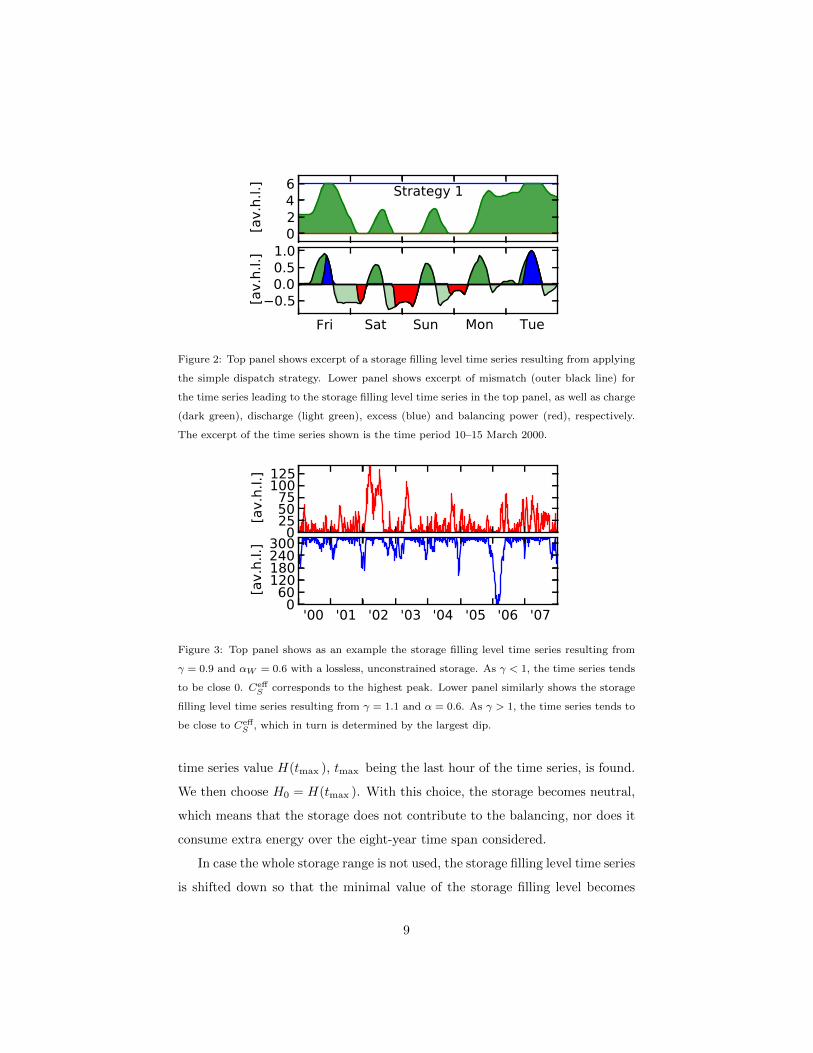
Figure 2: Top panel shows excerpt of a storage filling level time series resulting from applying

the simple dispatch strategy. Lower panel shows excerpt of mismatch (outer black line) for

the time series leading to the storage filling level time series in the top panel, as well as charge

(dark green), discharge (light green), excess (blue) and balancing power (red), respectively.

The excerpt of the time series shown is the time period 10–15 March 2000.

0255075

100125

[av.

h.l.]

'00 '01 '02 '03 '04 '05 '06 '07060

120180240300

[av.

h.l.]

Figure 3: Top panel shows as an example the storage filling level time series resulting from

γ = 0.9 and αW = 0.6 with a lossless, unconstrained storage. As γ < 1, the time series tends

to be close 0. CeffS corresponds to the highest peak. Lower panel similarly shows the storage

filling level time series resulting from γ = 1.1 and α = 0.6. As γ > 1, the time series tends to

be close to CeffS , which in turn is determined by the largest dip.

time series value H(tmax ), tmax being the last hour of the time series, is found.

We then choose H0 = H(tmax ). With this choice, the storage becomes neutral,

which means that the storage does not contribute to the balancing, nor does it

consume extra energy over the eight-year time span considered.

In case the whole storage range is not used, the storage filling level time series

is shifted down so that the minimal value of the storage filling level becomes

9

0. For a lossless storage (ηin = ηout = 1), this happens if the storage is large

enough to avoid additional average balancing. The effectively used storage size

CeffS is then given by maxtH(t). By choosing CS sufficiently large, making the

storage size in practice unconstrained, the algorithm can in this way be used to

determine the smallest storage size with the property that enlarging the storage

size has no effect on what can be stored or dispatched. Assuming lossless storage

with ηin = ηout = 1.00, the model with unconstrained storage size amounts to

storing all excess for γ ≤ 1, and exactly what is required to cover deficits for

γ ≥ 1. Figure 3 illustrates the storage filling level time series for unconstrained

storage sizes.

2.5. Reduced mismatch time series

So far, we have defined the generation and load time series, the mismatch

time series, the balancing time series and (additional) average balancing energy

as well as the storage filling level time series. To model the interaction of the

mismatch with the storage, we define a reduced mismatch time series, from

which we can determine how storage affects balancing needs.

The changes in the filling level of the storage can be described by the time

series F (t) given by:

F (t) = H(t)−H(t− 1) , t ≥ tmin . (8)

Correspondingly, the power flow in and out of the storage is

F (t) = η−1in F+(t)− ηoutF−(t) , (9)

where positive values indicate that power flows in and negative values indicate

that power flows out of the storage. We can now write the mismatch after

storage transactions as

∆r(t) = ∆(t)− F (t) , (10)

where “r” stands for “reduced.” The flows as well as the reduced mismatch

is illustrated in Figure 2 for a lossless storage. The reduced mismatch is now

10

0.0 0.5 1.0 1.5 2.0Average VRE generation factor γ

0.00

0.05

0.10

0.15

0.20

Ead

dB

αW =0.60αW =0.80Optimal αW

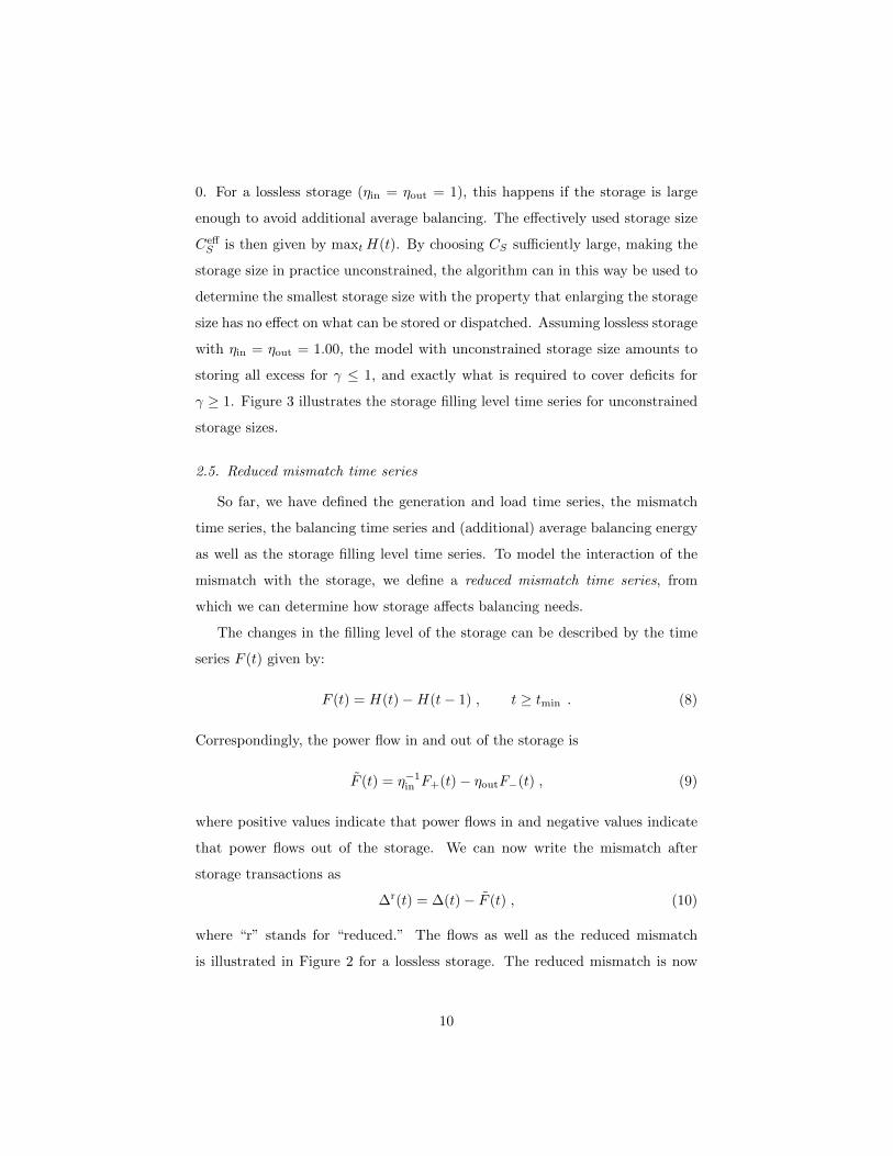
Figure 4: Additional average balancing EaddB vs. average VRE generation factor γ without

storage for αW = 0.60 (blue), αW = 0.80 (red) and the γ dependent optimal αW (gray).

used to find the balancing time series for scenarios with combined storage and

balancing, simply by

B(t) = ∆r−(t) . (11)

This definition replaces the previous definition (3) of the balancing time series. It

coincides with (3) when CS = 0. The definitions of EB and EaddB are unchanged.

A case of more than one storage, e.g. a small high-efficient short-term and

a larger low-efficient seasonal storage, can be modeled by feeding the reduced

mismatch time series resulting from the application of the smaller storage to

the model of the larger storage (see Sections 5 and 6).

3. The no storage and no additional average balancing scenarios

3.1. The no-storage scenario

Heide et al. (2011) has shown that in a scenario without storage and with

γ ≥ 1 the balancing needs are significant, even when the average VRE generation

exceeds the load, and when aggregated over all of Europe. With the improved

model presented here, we extend this scenario to the regime γ < 1.

11

0.0 0.5 1.0 1.5 2.0Average VRE generation factor γ

0.000.020.040.060.080.100.120.140.16

Stor

age

size

Cef

fS

[av.

y.l.] αW = 0.60

αW = 0.80Optimal αW

Figure 5: Storage singularity: Required storage size CeffS without additional average balancing

vs. average VRE power generation factor γ for αW = 0.60 (blue), αW = 0.80 and the γ-

dependent optimal αW (gray).

As revealed in Figure 4 the integration of wind and solar power works well up

to around γ = 0.5. Almost no additional average balancing is required up to this

penetration. Above this limit large amounts of additional average balancing are

required. Some of the generated power is potentially lost as excess generation,

if it is not stored or if a new use for highly intermittent power is not found.

The additional average balancing fraction EaddB strongly peaks at γ = 1. The

size of the peak strongly depends on the mix αW . For αW = 0.8 it becomes

a minimum. Also for γ 6= 1 the mix αW = 0.8 remains close to optimal. The

optimal αW minimizes balancing energy when no storage is present, cf. Heide

et al. (2011), and turns out to be γ dependent. The numerical value of the

optimal mix changes from 0.82 at γ = 0.5 via 0.80 at γ = 1.00 to 0.88 at

γ = 2.00.

3.2. The no additional average balancing scenario

As already explored for γ ≥ 1 in Heide et al. (2010, 2011), the alternative

scenario where additional average balancing is completely avoided by storing

12

enough excess generation to cover additional average balancing needs, leads to

very large storage sizes. Using the extended model, we can also cover γ < 1. At

equilibrium (∑

t ∆(t) = 0), which for lossless storages is reached at γ = 1.00, a

pronounced cusp singularity of required storage size appears. See Figure 5.

The choices of mix in Figure 5 reflect the findings of Heide et al. (2010, 2011),

with the mix αW = 0.60 minimizing storage at γ = 1.00 and the mix αW = 0.80

minimizing balancing at γ = 1.00. Here, the optimal αW is the γ dependent

choice that minimizes the storage size without introducing additional average

balancing. This optimal mix varies between 0.55 and 0.78 and is different from

the optimal mix discussed in the previous subsection.

As seen in the figure, also for γ < 1 the storage size resulting from the mix

αW = 0.60 is very close to the result for the optimal mix, and significantly better

than that of the mix αW = 0.80. When γ gets larger than 1, the αW = 0.60 and

αW = 0.80 cases quickly get very close to each other, reflecting the fact that, as

excess generation increases, it is easier to keep the storage filled up and deficits

become more rare, regardless of the mix. The case of optimal mix, however,

performs slightly better in the γ range 1.00–1.50.

4. Combined usage of lossless storage and balancing

In this section, we investigate the advantages of combining storage and bal-

ancing. The scenarios described in Section 3 are extreme cases of a more general

setup where storage and balancing are used in combination. In between the ex-

tremal balancing and storage scenarios, there is an unlimited number of possible

combined balancing and storage strategies. In this paper, we will restrict our-

selves to storage first strategies, with an imposed limit on the storage size, and

balancing handling any remaining mismatch as described in Section 2. This

class of strategies can be parametrized by the given storage size. They include

the extremal balancing and storage scenarios as special cases by setting the im-

posed storage size limit to 0 or sufficiently large, respectively. A key property

of the storage first strategies is that they minimize the additional average bal-

13

0 6 12 18 24Storage size CS [av.h.l.]

0.00

0.05

0.10

0.15

0.20

Ead

dB

100 101 102 1030.000.050.100.150.20 γ=0.75

γ=1.00γ=1.25

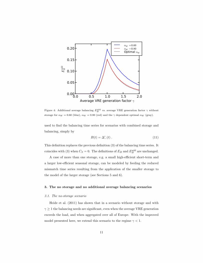
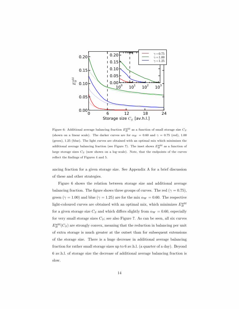
Figure 6: Additional average balancing fraction EaddB as a function of small storage size CS

(shown on a linear scale). The darker curves are for αW = 0.60 and γ = 0.75 (red), 1.00

(green), 1.25 (blue). The light curves are obtained with an optimal mix which minimizes the

additional average balancing fraction (see Figure 7). The inset shows EaddB as a function of

large storage sizes CS (now shown on a log–scale). Note, that the endpoints of the curves

reflect the findings of Figures 4 and 5.

ancing fraction for a given storage size. See Appendix A for a brief discussion

of these and other strategies.

Figure 6 shows the relation between storage size and additional average

balancing fraction. The figure shows three groups of curves. The red (γ = 0.75),

green (γ = 1.00) and blue (γ = 1.25) are for the mix αW = 0.60. The respective

light-coloured curves are obtained with an optimal mix, which minimizes EaddB

for a given storage size CS and which differs slightly from αW = 0.60, especially

for very small storage sizes CS ; see also Figure 7. As can be seen, all six curves

EaddB (CS) are strongly convex, meaning that the reduction in balancing per unit

of extra storage is much greater at the outset than for subsequent extensions

of the storage size. There is a huge decrease in additional average balancing

fraction for rather small storage sizes up to 6 av.h.l. (a quarter of a day). Beyond

6 av.h.l. of storage size the decrease of additional average balancing fraction is

slow.

14

0 6 12 18 24Storage size CS [av.h.l.]

0.0

0.2

0.4

0.6

0.8

1.0

Win

d fra

ctio

n αW

γ=0.75γ=1.00γ=1.25

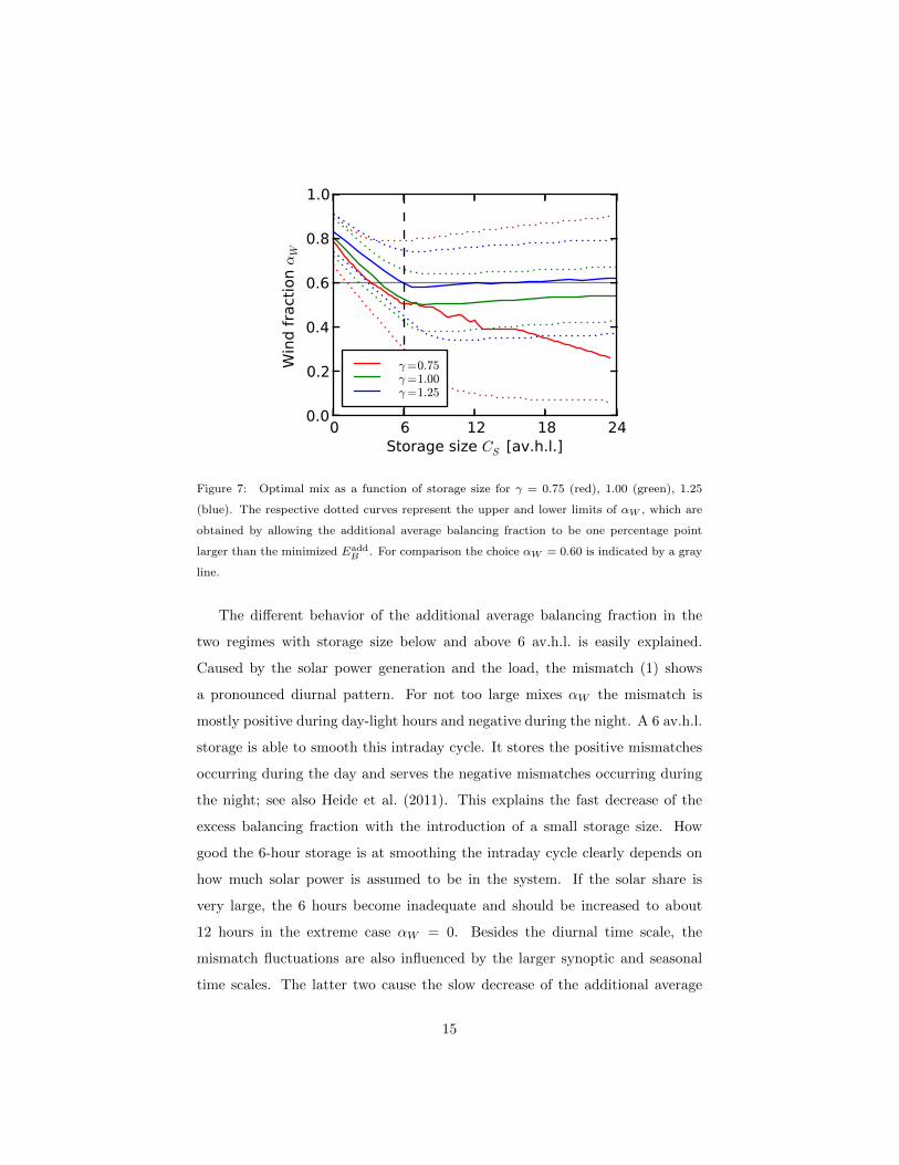
Figure 7: Optimal mix as a function of storage size for γ = 0.75 (red), 1.00 (green), 1.25

(blue). The respective dotted curves represent the upper and lower limits of αW , which are

obtained by allowing the additional average balancing fraction to be one percentage point

larger than the minimized EaddB . For comparison the choice αW = 0.60 is indicated by a gray

line.

The different behavior of the additional average balancing fraction in the

two regimes with storage size below and above 6 av.h.l. is easily explained.

Caused by the solar power generation and the load, the mismatch (1) shows

a pronounced diurnal pattern. For not too large mixes αW the mismatch is

mostly positive during day-light hours and negative during the night. A 6 av.h.l.

storage is able to smooth this intraday cycle. It stores the positive mismatches

occurring during the day and serves the negative mismatches occurring during

the night; see also Heide et al. (2011). This explains the fast decrease of the

excess balancing fraction with the introduction of a small storage size. How

good the 6-hour storage is at smoothing the intraday cycle clearly depends on

how much solar power is assumed to be in the system. If the solar share is

very large, the 6 hours become inadequate and should be increased to about

12 hours in the extreme case αW = 0. Besides the diurnal time scale, the

mismatch fluctuations are also influenced by the larger synoptic and seasonal

time scales. The latter two cause the slow decrease of the additional average

15

balancing fraction for storage sizes beyond 6 av.h.l.

Note that the optimal mix between wind and solar power generation is

also different for the two storage regimes (cf. Figure 7). Sufficiently below the

6 av.h.l. storage size, the optimal mix is αW ' 0.8, and the balancing energy in-

creases relatively rapidly, as one deviates from the optimum value, as indicated

by the dotted lines in Figure 7. This is a consequence mostly of the fact that the

strong diurnal patterns of solar power makes it difficult to integrate large quan-

tities of it into the power system without storage. At 6 av.h.l. the optimal mix

has decreased to αW = 0.5− 0.6 and the range of mixes that result in approx-

imately the same balancing has increased significantly. For larger storage sizes

the mix 0.6 results in a balancing energy close to the optimal mix for all γ’s. In

this regime the optimal mix is no longer sensitive to fluctuations on the diurnal

time scale. It is dominated by the fluctuations occurring on the seasonal time

scale. We note that the optimal mix αW = 0.60 differs from what is indicated

in Schaber et al. (2012b) where a mix of 0.80 is suggested to be optimal in the

presence of storage and a large VRE penetration.6 As the αW = 0.60 curves are

good approximators of the optimal mix curves for storages larger than 6 av.h.l.,

we will focus on this choice in what follows.

5. A lossless 6-hour storage with unconstrained balancing and sea-

sonal storage

As described above, the introduction of a 6-hour storage has a significant

impact on the required balancing energy as compared to no storage. Contrary

to the enormous storage sizes needed in the full storage scenario (cf. Fig. 5),

a 6-hour storage also appears to be technically feasible. Storages of that or-

der may be realized by a combination of many different storage and time-shift

6This due to the fact that the measure used in Schaber et al. (2012b), which can be defined

as D =∑

t|∆(t)|, has no temporal memory. This means that, in principle, the storage could

be full all summer and empty all winter, resulting in 1 yearly storage cycle, and still result in

a small D.

16

technologies such as pumped hydro, compressed air, superconducting magnetic

energy storages, different battery technologies, flywheels, capacitors (Beaudin

et al. (2010)) and demand side management and smart grid (Strbac (2008)).

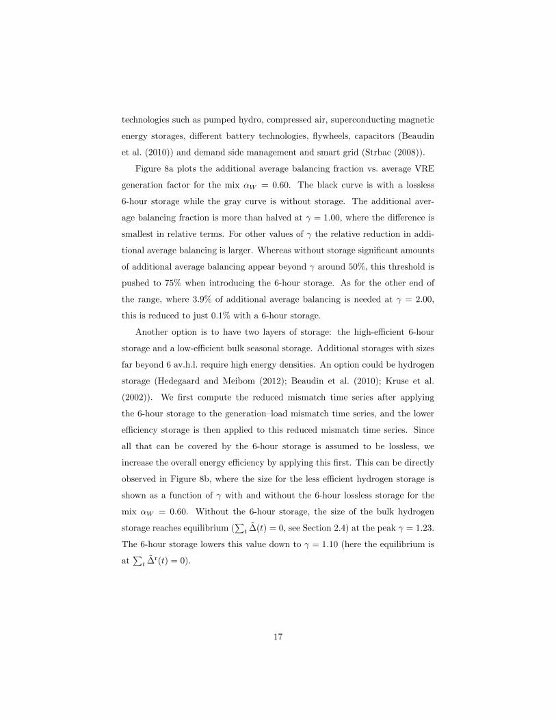
Figure 8a plots the additional average balancing fraction vs. average VRE

generation factor for the mix αW = 0.60. The black curve is with a lossless

6-hour storage while the gray curve is without storage. The additional aver-

age balancing fraction is more than halved at γ = 1.00, where the difference is

smallest in relative terms. For other values of γ the relative reduction in addi-

tional average balancing is larger. Whereas without storage significant amounts

of additional average balancing appear beyond γ around 50%, this threshold is

pushed to 75% when introducing the 6-hour storage. As for the other end of

the range, where 3.9% of additional average balancing is needed at γ = 2.00,

this is reduced to just 0.1% with a 6-hour storage.

Another option is to have two layers of storage: the high-efficient 6-hour

storage and a low-efficient bulk seasonal storage. Additional storages with sizes

far beyond 6 av.h.l. require high energy densities. An option could be hydrogen

storage (Hedegaard and Meibom (2012); Beaudin et al. (2010); Kruse et al.

(2002)). We first compute the reduced mismatch time series after applying

the 6-hour storage to the generation–load mismatch time series, and the lower

efficiency storage is then applied to this reduced mismatch time series. Since

all that can be covered by the 6-hour storage is assumed to be lossless, we

increase the overall energy efficiency by applying this first. This can be directly

observed in Figure 8b, where the size for the less efficient hydrogen storage is

shown as a function of γ with and without the 6-hour lossless storage for the

mix αW = 0.60. Without the 6-hour storage, the size of the bulk hydrogen

storage reaches equilibrium (∑

t ∆(t) = 0, see Section 2.4) at the peak γ = 1.23.

The 6-hour storage lowers this value down to γ = 1.10 (here the equilibrium is

at∑

t ∆r(t) = 0).

17

0.0 0.5 1.0 1.5 2.0Average VRE generation factor γ

0.00

0.05

0.10

0.15

0.20

Ead

dB

With 6 h storageNo 6 h storage

0.0 0.5 1.0 1.5 2.0Average VRE generation factor γ

0.00

0.02

0.04

0.06

0.08

0.10

0.12

Stor

age

size

Cef

fS

[av.

y.l.]

25 TWh

With 6 h storageNo 6 h storage

Figure 8: (a) additional average balancing fraction EaddB and (b) storage size Ceff

S for a

hydrogen storage vs. average VRE power generation factor γ with (black) and without (gray)

first using a 6-hour lossless storage for αW = 0.60.

6. A lossless 6-hour storage with constrained hydro balancing and

hydrogen storage

A possible way of providing a renewable form of balancing that can be

dispatched on demand is to use the hydro power storage lakes of northern

Scandinavia, the Alps and elsewhere in Europe. In France, Italy, Spain and

18

Switzerland alone, the current generation from storage lake facilities amounts

to about 70 TWh/yr, and the total hydro power generation of Norway and

Sweden amounts to 190 TWh/yr, most of which is generated from storage lake

facilities (Lehner et al. (2005)). Here, we assume that at least 150 TWh/yr of

the total European hydro power generation can be dispatched on demand. This

amounts to about 5% of the average load, and to the best of our knowledge,

it represents a conservative estimate. As an alternative to hydro power, other

sources of dispatchable renewable balancing such as biomass fired power plants

could also be assumed without changing the conclusions of the analysis.

Bulk seasonal storage in a fully renewable pan-European power system could

be realized as e.g. underground hydrogen storage. Of the different types of un-

derground storage types presently used for natural gas, only solution mined salt

caverns are directly usable for hydrogen storage (Stone et al. (2009)). In Europe

most of the suitable geological formations are located in northern Germany, and

the combined working gas volume of all existing European facilities allows for

storage of 32.5 TWh in the form of hydrogen (Gilhaus (2007)). In the following

we assume that a total storage size of 25 TWh are made available for hydrogen

storage and we use conversion efficiencies of ηin = ηout = 0.60.

With a total balancing energy of 150 TWh/yr and a 25 TWh hydrogen

storage, as described above, we model the optimal combined operation with and

without an additional lossless 6-hour storage (2.2 TWh). As outlined at the end

of Section 2, first the high-efficient 6-hour storage, if included, is applied to the

mismatch time series, next the reduced mismatch time series is confronted with

the constrained hydrogen storage, and finally, the still existing (doubly reduced)

mismatch determines the balancing needs. According to Figure 8b, for the mix

αW = 0.60 the storage size of 25 TWh (corresponding to 0.008 av.y.l. in 2007-

units) only represents a constraint for average VRE power generation factors γ

between 0.97 and 1.80 without a 6-hour storage and between 0.92 and 1.55 with

a 6-hour storage.

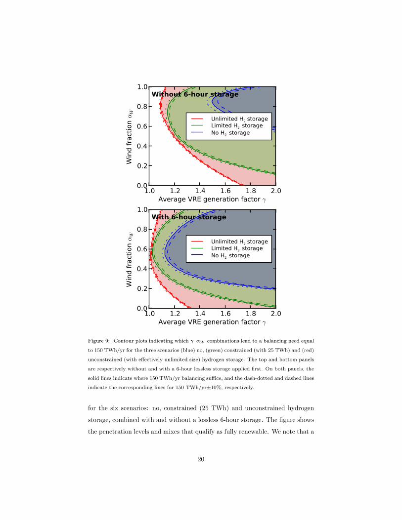
Now the question is which combinations of γ and αW satisfy the 150 TWh/yr

constraint of hydro balancing. The answer to this question is given in Figure 9

19

1.0 1.2 1.4 1.6 1.8 2.0Average VRE generation factor γ

0.0

0.2

0.4

0.6

0.8

1.0

Win

d fra

ctio

n αW

Without 6-hour storage

Unlimited H2 storageLimited H2 storageNo H2 storage

1.0 1.2 1.4 1.6 1.8 2.0Average VRE generation factor γ

0.0

0.2

0.4

0.6

0.8

1.0

Win

d fra

ctio

n αW

With 6-hour storage

Unlimited H2 storageLimited H2 storageNo H2 storage

Figure 9: Contour plots indicating which γ–αW combinations lead to a balancing need equal

to 150 TWh/yr for the three scenarios (blue) no, (green) constrained (with 25 TWh) and (red)

unconstrained (with effectively unlimited size) hydrogen storage. The top and bottom panels

are respectively without and with a 6-hour lossless storage applied first. On both panels, the

solid lines indicate where 150 TWh/yr balancing suffice, and the dash-dotted and dashed lines

indicate the corresponding lines for 150 TWh/yr±10%, respectively.

for the six scenarios: no, constrained (25 TWh) and unconstrained hydrogen

storage, combined with and without a lossless 6-hour storage. The figure shows

the penetration levels and mixes that qualify as fully renewable. We note that a

20

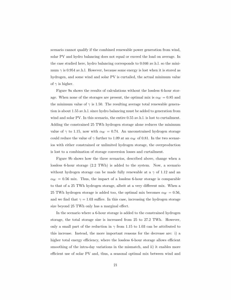
scenario cannot qualify if the combined renewable power generation from wind,

solar PV and hydro balancing does not equal or exceed the load on average. In

the case studied here, hydro balancing corresponds to 0.046 av.h.l. so the mini-

mum γ is 0.954 av.h.l. However, because some energy is lost when it is stored as

hydrogen, and some wind and solar PV is curtailed, the actual minimum value

of γ is higher.

Figure 9a shows the results of calculations without the lossless 6-hour stor-

age. When none of the storages are present, the optimal mix is αW = 0.85 and

the minimum value of γ is 1.50. The resulting average total renewable genera-

tion is about 1.55 av.h.l. since hydro balancing must be added to generation from

wind and solar PV. In this scenario, the entire 0.55 av.h.l. is lost to curtailment.

Adding the constrained 25 TWh hydrogen storage alone reduces the minimum

value of γ to 1.15, now with αW = 0.74. An unconstrained hydrogen storage

could reduce the value of γ further to 1.09 at an αW of 0.81. In the two scenar-

ios with either constrained or unlimited hydrogen storage, the overproduction

is lost to a combination of storage conversion losses and curtailment.

Figure 9b shows how the three scenarios, described above, change when a

lossless 6-hour storage (2.2 TWh) is added to the system. Now, a scenario

without hydrogen storage can be made fully renewable at a γ of 1.12 and an

αW = 0.56 mix. Thus, the impact of a lossless 6-hour storage is comparable

to that of a 25 TWh hydrogen storage, albeit at a very different mix. When a

25 TWh hydrogen storage is added too, the optimal mix becomes αW = 0.56,

and we find that γ = 1.03 suffice. In this case, increasing the hydrogen storage

size beyond 25 TWh only has a marginal effect.

In the scenario where a 6-hour storage is added to the constrained hydrogen

storage, the total storage size is increased from 25 to 27.2 TWh. However,

only a small part of the reduction in γ from 1.15 to 1.03 can be attributed to

this increase. Instead, the more important reasons for the decrease are: i) a

higher total energy efficiency, where the lossless 6-hour storage allows efficient

smoothing of the intra-day variations in the mismatch, and ii) it enables more

efficient use of solar PV and, thus, a seasonal optimal mix between wind and

21

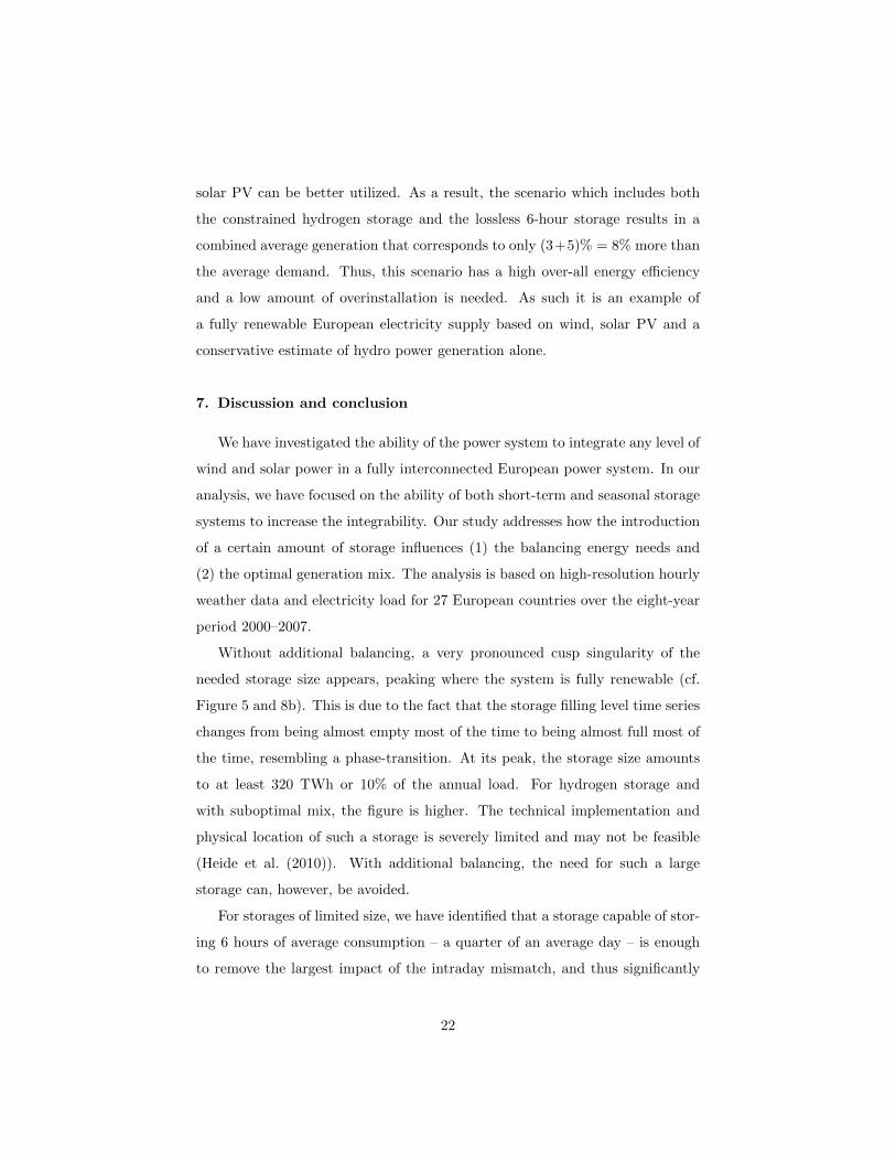
solar PV can be better utilized. As a result, the scenario which includes both

the constrained hydrogen storage and the lossless 6-hour storage results in a

combined average generation that corresponds to only (3+5)% = 8% more than

the average demand. Thus, this scenario has a high over-all energy efficiency

and a low amount of overinstallation is needed. As such it is an example of

a fully renewable European electricity supply based on wind, solar PV and a

conservative estimate of hydro power generation alone.

7. Discussion and conclusion

We have investigated the ability of the power system to integrate any level of

wind and solar power in a fully interconnected European power system. In our

analysis, we have focused on the ability of both short-term and seasonal storage

systems to increase the integrability. Our study addresses how the introduction

of a certain amount of storage influences (1) the balancing energy needs and

(2) the optimal generation mix. The analysis is based on high-resolution hourly

weather data and electricity load for 27 European countries over the eight-year

period 2000–2007.

Without additional balancing, a very pronounced cusp singularity of the

needed storage size appears, peaking where the system is fully renewable (cf.

Figure 5 and 8b). This is due to the fact that the storage filling level time series

changes from being almost empty most of the time to being almost full most of

the time, resembling a phase-transition. At its peak, the storage size amounts

to at least 320 TWh or 10% of the annual load. For hydrogen storage and

with suboptimal mix, the figure is higher. The technical implementation and

physical location of such a storage is severely limited and may not be feasible

(Heide et al. (2010)). With additional balancing, the need for such a large

storage can, however, be avoided.

For storages of limited size, we have identified that a storage capable of stor-

ing 6 hours of average consumption – a quarter of an average day – is enough

to remove the largest impact of the intraday mismatch, and thus significantly

22

reduce the balancing energy needs (cf. Figure 8). This implies that the opti-

mal mix is shifted towards the seasonal optimal mix. A high-efficiency 6-hour

storage more than halves the balancing energy needs at γ = 1.00 for a mix of

αW = 0.60. The impact is even greater for both higher and lower penetration

levels, allowing for full integration up to an average combined wind and solar

power generation of about 75% (cf. Figure 8a). Without the 6-hour storage,

this full integration can only be achieved up to about 50% for a fully connected

Europe. As indicated in Figure 9, the impact of a 6-hour lossless storage (at

optimal mix) is under certain circumstances almost as good as an unlimited

hydrogen storage (at optimal mix). As opposed to the 320 TWh storage de-

scribed above, a 6-hour storage, which corresponds to 2.2 TWh, can be realized

by combining many different technological solutions including physical storages

and time-shift technologies. Our results indicate that political support for the

development of such technologies will be very beneficial for the system when the

VRE penetration reaches 50% and will continue to have a great impact even in

the fully renewable regime.

A seasonal storage can most likely only be realized with a low round-trip

efficiency. A low-efficiency storage with a round-trip efficiency of 0.36 (0.60

each direction) and a storage size of 25 TWh (capable of providing up to 0.60 ·

25 TWh = 15 TWh of stored energy), is technically realizable e.g. as hydrogen

stored in solution mined salt caverns in northern Germany. In this scenario,

the high-efficiency 6-hour storage serves the purpose of reducing the conversion

losses, making the 150 TWh/yr of balancing sufficient for a γ of just 1.03 at

an αW = 0.56 mix (again, cf. Figure 9). Without the 6-hour storage, the

corresponding number would be γ = 1.15 (αW = 0.80 mix). Two fully renewable

scenarios can be realized with a lossless 6-hour storage: one with γ = 1.03 and

a 25 TWh hydrogen storage and one with γ = 1.12 and no additional storage.

Whether there should be a hydrogen storage depends on the price of the 25 TWh

compared to the price of going from γ = 1.03 to γ = 1.12, be it measured in

environmental impact, economical terms or otherwise. If a highly efficient short-

term storage comparable to our 6-hour storage does not become feasible, the

23

impact of a hydrogen storage is much greater, as it reduces the needed γ from

1.52 to 1.15 or 1.09, depending on whether the storage is limited to 25 TWh or

not.

In conclusion, we find a significant synergy between storage and balancing.

In particular, the effect of a highly efficient short-term storage dramatically re-

duces the balancing energy needs and allows for efficient use of a mix close to

the seasonal optimal mix of wind and solar power. However, the additional gain

by increasing the storage size of such a storage further is limited. A seasonal

storage will most likely have a low efficiency, but in combination with a highly

efficient short-term storage, the efficiency of the combined storage system is in-

creased. This reduces the needed amount of overproduction in a fully renewable

scenario. With a balancing of only 150 TWh/yr, e.g. coming from biomass or

hydro power, a highly efficient 6-hour storage and a 25 TWh hydrogen storage

employed, we find that a fully renewable scenario can be realized with an aver-

age wind and solar power production of only 3% more than the average load.

Increasing the hydrogen storage size further does not lower the needed amount

of overproduction substantially, and increasing the figure to 12%, a hydrogen

storage can be completely avoided.

At present, the intracontinental power grid is becoming a bottleneck for

the integration of non-dispatchable renewables such as wind and solar power.

We find that even with a perfect grid, a combined penetration of wind and

solar power of about 50% will lead to the need for an energy storage in order

to avoid large losses. Investment in an efficient (virtual or physical) storage

able to store the average demand for 6 hours is very important as it bears

large benefits. However, we find that building a storage large enough to handle

all surplus generation at large penetrations is unfeasible. A moderately large

storage provides almost the same benefits, in particular in combination with the

highly efficient small storage.

24

Acknowledgements

We would like to thank Rolando A. Rodriguez for proofreading several earlier

versions of this manuscript and the two anonymous referees for comments that

markedly improved the quality of this final paper. The first author was sup-

ported by the Carlsberg Foundation during all stages of the work. The second

author is supported by DONG Energy.

Aboumahboub, T., Schaber, K., Tzscheutschler, P., Hamacher, T., 2010. Op-

timal configuration of a renewable-based electricity supply sector. WSEAS

Transactions on Power Systems 5, 120–129.

Beaudin, M., Zareipour, H., Schellenberglabe, A., Rosehart, W., 2010. Energy

storage for mitigating the variability of renewable electricity sources: An

updated review. Energy for Sustainable Development 14, 302–314.

Czisch, G., 2005. Szenarien zur zukunftigen Stromversorgung, kostenoptimierte

Variationen zur Versorgung Europas und seiner Nachbarn mit Strom aus

erneuerbaren Energien. Ph.D. thesis. Universitat Kassel.

Czisch, G., Giebel, G., 2007. Realisable scenarios for a future electricity supply

based 100% on renewable energies, in: Energy Solutions for Sustainable De-

velopment Proceedings Risø International Energy Conference, Risø National

Library, Technical University of Denmark. pp. 186–195.

ECF, 2010. Roadmap 2050: A practical guide to a prosperous, low-carbon

Europe. Report. European Climate Foundation.

Gilhaus, A., 2007. Natural Gas Storage in Salt Caverns – Present Status, Devel-

opments and Future Trends in Europe. Technical Conference Paper. Solution

Mining Research Institute.

Hedegaard, K., Meibom, P., 2012. Wind power impacts and electricity storage

– a time scale perspective. Renewable Energy 37, 318–324.

25

Heide, D., von Bremen, L., Greiner, M., Hoffmann, C., Speckmann, M., Bofin-

ger, S., 2010. Seasonal optimal mix of wind and solar power in a future, highly

renewable europe. Renewable Energy 35, 2483–2489.

Heide, D., Greiner, M., von Bremen, L., Hoffmann, C., 2011. Reduced storage

and balancing needs in a fully renewable european power system with excess

wind and solar power generation. Renewable Energy 36, 2515–2523.

Jacobson, M.Z., Delucchi, M.A., 2011. Providing all global energy with wind,

water, and solar power, part I: Technologies, energy resources, quantities and

areas of infrastructure, and materials. Energy Policy 39, 1154–1169.

Kempton, W., Pimenta, F.M., Veron, D.E., Colle, B.A., 2010. Electric power

from offshore wind via synoptic scale interconnection. PNAS 107, 7240–7245.

Kruse, B., Grinna, S., Buch, C., 2002. Hydrogen – Status og muligheter. Tech-

nical Report 6. Bellona. (in English).

Lehner, B., Czisch, G., Vassolo, S., 2005. The impact of global change on the

hydropower potential of Europe: A model based analysis. Energy Policy 33,

839–855.

Lund, H., Mathiesen, B.V., 2009. Energy system analysis of 100% renewable

energy systems – The case of Denmark in years 2030 and 2050. Energy 34,

524–531.

Martinot, E., Dienst, C., Weiliang, L., Qimin, C., 2007. Renewable energy

futures: Targets, scenarios, and pathways. Annual Review of Environment

and Resources 32, 205–239.

Rodriguez, R., Andresen, G.B., Becker, S., Greiner, M., 2012. Transmission

needs in a fully renewable pan-European electricity system, in: Uyar, T.S.,

Saglam, M., Sulukan, E. (Eds.), 2nd International 100% Renewable Energy

Conference and Exhibition (IRENEC 2012) Proceedings, Maltepe – Istanbul,

Turkey. pp. 320–324.

26

Schaber, K., Steinke, F., Hamacher, T., 2012a. Transmission grid extensions for

the integration of variable renewable energies in europe: Who benefits where?

Energy Policy 43, 123–135.

Schaber, K., Steinke, F., Muhlich, P., Hamacher, T., 2012b. Parametric study

of variable renewable energy integration in europe: Advantages and costs of

transmission grid extensions. Energy Policy 42, 498–508.

Stone, H.B.J., Veldhuis, I., Richardson, R.N., 2009. Underground hydrogen

storage in the UK. The Geological Society, London, Special Publications 313,

217–226.

Strbac, G., 2008. Demand side management: Benefits and challenges. Energy

Policy 36.

Widen, J., 2011. Correlations between large-scale solar and wind power in a

future scenario for Sweden. IEEE Transactions on Sustainable Energy 2,

177–184.

Yao, R., Steemers, K., 2005. A method of formulating energy load profile for

domestic buildings in the UK. Energy and Buildings 37, 663–671.

Appendix A. Strategies

In this appendix, we discuss the optimality of the “storage first” strategy

with regard to balancing minimization for a given storage size and give a few

examples of other strategies with other optimality properties. The fact that the

“storage first” strategy is indeed optimal with respect to minimizing balancing

energy follows from a simple induction argument, which is left to the interested

reader as an easy exercise for the mathematically trained.

We stress that this strategy is not the only optimal strategy in this respect.

Recall that the presented storage first strategy acts on an hour-by-hour basis by

using the storage to cover deficits in the generation–load mismatch time series if

the storage is not empty, and balancing in case the storage is or runs empty, and

27

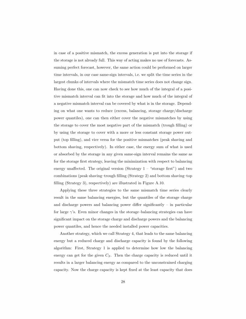
in case of a positive mismatch, the excess generation is put into the storage if

the storage is not already full. This way of acting makes no use of forecasts. As-

suming perfect forecast, however, the same action could be performed on larger

time intervals, in our case same-sign intervals, i.e. we split the time series in the

largest chunks of intervals where the mismatch time series does not change sign.

Having done this, one can now check to see how much of the integral of a posi-

tive mismatch interval can fit into the storage and how much of the integral of

a negative mismatch interval can be covered by what is in the storage. Depend-

ing on what one wants to reduce (excess, balancing, storage charge/discharge

power quantiles), one can then either cover the negative mismatches by using

the storage to cover the most negative part of the mismatch (trough filling) or

by using the storage to cover with a more or less constant storage power out-

put (top filling), and vice versa for the positive mismatches (peak shaving and

bottom shaving, respectively). In either case, the energy sum of what is used

or absorbed by the storage in any given same-sign interval remains the same as

for the storage first strategy, leaving the minimization with respect to balancing

energy unaffected. The original version (Strategy 1 – “storage first”) and two

combinations (peak shaving–trough filling (Strategy 2) and bottom shaving–top

filling (Strategy 3), respectively) are illustrated in Figure A.10.

Applying these three strategies to the same mismatch time series clearly

result in the same balancing energies, but the quantiles of the storage charge

and discharge powers and balancing power differ significantly – in particular

for large γ’s. Even minor changes in the storage–balancing strategies can have

significant impact on the storage charge and discharge powers and the balancing

power quantiles, and hence the needed installed power capacities.

Another strategy, which we call Strategy 4, that leads to the same balancing

energy but a reduced charge and discharge capacity is found by the following

algorithm: First, Strategy 1 is applied to determine how low the balancing

energy can get for the given CS . Then the charge capacity is reduced until it

results in a larger balancing energy as compared to the unconstrained charging

capacity. Now the charge capacity is kept fixed at the least capacity that does

28

0246

[av.

h.l.] Strategy 1

Fri Sat Sun Mon Tue0.50.00.51.0

[av.

h.l.]

0246

[av.

h.l.] Strategy 2

Fri Sat Sun Mon Tue0.50.00.51.0

[av.

h.l.]

0246

[av.

h.l.] Strategy 3

Fri Sat Sun Mon Tue0.50.00.51.0

[av.

h.l.]

Figure A.10: Storage filling level (top panels) and mismatch, storage flow, excess and bal-

ancing power (bottom panels) for Strategies 1, 2 and 3, respectively. The positive mismatch

is divided into a dark green and a blue part: Dark green is stored, while blue is excess power

not absorbed by storage. Likewise, the negative mismatch is divided into a light green and

a red part: Light green is covered by storage while the red represents coverage by balancing.

The excerpt of the time series shown is the time period 10–15 March 2000.

not affect the balancing energy, while the discharge capacity is reduced until it

results in larger balancing energy.

A suboptimal strategy along the same lines, Strategy 5, can be defined as

29

0246

[av.

h.l.] Strategy 4

Fri Sat Sun Mon Tue0.50.00.51.0

[av.

h.l.]

0246

[av.

h.l.] Strategy 5

Fri Sat Sun Mon Tue0.50.00.51.0

[av.

h.l.]

Figure A.11: Storage filling level (top panels) and mismatch, storage flow, excess and balanc-

ing power (bottom panels) for Strategies 4 and 5, respectively. See Figure A.10 for explanation

of the color coding.

Strategy 4, but with the difference that a slightly higher balancing energy, say

10% larger, is allowed. Strategies 4 and 5 are illustrated in Figure A.11. In

this concrete example, where the balancing energy is allowed to be 10% larger

(EB = 0.1 instead of EB = 0.09) for Strategy 5, γ = 1.0 and αW = 0.6,

the storage charge and discharge capacities are both approximately halved as

compared to Strategy 4, and compared to the other strategies, the difference is

even larger.

We will not pursue this issue any further in this paper, as a more complex

model including transmission and storage sites seems to be needed in order to

give useful results.

30