International Review of Business Research Papers Vol. 5 No. 4 June 2009 Pp. 426-447 Stock Return, Volatility And The Global Financial Crisis In

An Emerging Market: The Nigerian Case

Olowe, Rufus Ayodeji1

This paper investigated the relation between stock returns

and volatility in Nigeria using E-GARCH-in-mean model in the light of banking reforms, insurance reform, stock market crash and the global financial crisis. Using daily returns over the period 4 January 2004 to January 9, 2009, Volatility persistence, asymmetric properties and risk-return relationship are investigated for the Nigerian stock market. The result also shows that volatility is persistent and there is leverage effect supporting the work of Nelson (1991) .The study found little evidence on the relationship between stock returns and risk as measured by its own volatility. The study found positive but insignificant relationship between stock return and risk. The result shows the banking reform in July 2004 and stock market crash since April 2008 negatively impacts on stock return while insurance reform and the global financial crisis have no impact on stock return. The stock market crash of 2008 is found to have contributed to the high volatility persistence in the Nigerian stock market especially during the global financial crisis period. The stock market crash is also found to have accounted for the sudden change in variance.

Field of Research: Stock market, Financial Reforms, Global Financial crisis,

Volatility persistence, E-GARCH-in-mean, Risk-return tradeoff 1. Introduction Recently, the volatility of the stock market return on the Nigerian stock market has been of concern to investors, analysts, brokers, dealers and regulators. Stock return volatility which represents the variability of stock price changes could be perceived as a measure of risk. The understanding of the volatility in a stock market will be useful in the determination of the cost of capital and in the evaluation of asset allocation decisions. Policy makers therefore rely on market estimates of volatility as a barometer of the vulnerability of financial markets. However, the existence of excessive volatility, or “noise,” in the stock market undermines the usefulness of stock prices as a “signal” about the true intrinsic value of a firm, a concept that is core to the paradigm of the informational efficiency of markets (Karolyi, 2001). The traditional measure of volatility as represented by variance or standard deviation is unconditional and does not recognize that there are interesting patterns in asset volatility; e.g., time-varying and clustering properties. Researchers have introduced various models to explain and predict these patterns in volatility. Engle (1982) introduced the autoregressive conditional heteroskedasticity (ARCH) to model volatility. Engle (1982) modeled the heteroskedasticity by relating the conditional 1 Department of finance, University of Lagos, Akoka, Lagos, Nigeria. E-mail: raolowe@yahoo.co.uk

Olowe

427

variance of the disturbance term to the linear combination of the squared disturbances in the recent past. Bollerslev (1986) generalized the ARCH model by modeling the conditional variance to depend on its lagged values as well as squared lagged values of disturbance, which is called generalized autoregressive conditional heteroskedasticity (GARCH). Some of the models include IGARCH originally proposed by Engle and Bollerslev (1986), GARCH-in-Mean (GARCH-M) model introduced by Engle, Lilien and Robins (1987),the standard deviation GARCH model introduced by Taylor (1986) and Schwert (1989), the EGARCH or Exponential GARCH model proposed by Nelson (1991), TARCH or Threshold ARCH and Threshold GARCH were introduced independently by Zakoïan (1994) and Glosten, Jaganathan, and Runkle (1993), the Power ARCH model generalised by Ding,. Zhuanxin, C. W. J. Granger, and R. F. Engle (1993) among others. If investors are risk averse, theory predicts a positive relationship should exist between stock return and volatility (Leon, 2007). If there is a high volatility in a stock market, the investors should be compensated in form of higher risk premium. The GARCH-in-Mean (GARCH-M) model introduced by Engle, Lilien and Robins (1987) has been used by various researchers to examine the relationship between stock return and volatility (see French, Schwert and Stambaugh ,1987; Chou, 1988; Baillie and DeGennaro ,1990; Nelson, 1991; Glosten et al., 1993, Léon, 2007 among others). Mixed results were found by various authors. Some found the relation between the risk and return to be positive (French, Schwert and Stambaugh ,1987; Chou, 1988;among others) while some others found it negative (Nelson, 1991; Glosten et al., 1993 among others).Little or no work has been done on modeling stock returns volatility in Nigeria particularly using GARCH models. This paper attempts to fill this gap. The recapitalization of the banking industry in Nigeria in July 2004 and the Insurance industry in September 2005 boosted the number of securities on Nigerian stock market increasing public awareness and confidence about the Stock market. The increased trading activity on the stock market could have affected the volatility of the stock market. However, since April 1, 2008, investors have been worried about the falling stock prices on the Nigerian stock market. The global financial crisis of 2008 , an ongoing major financial crisis, could have affected stock volatility. The crisis which was triggered by the subprime mortgage crisis in the United States became prominently visible in September 2008 with the failure, merger, or conservatorship of several large United States-based financial firms exposed to packaged subprime loans and credit default swaps issued to insure these loans and their issuers (Wikipedia, 2009). The crisis rapidly evolved into a global credit crisis, deflation and sharp reductions in shipping and commerce, resulting in a number of bank failures in Europe and sharp reductions in the value of equities (stock) and commodities worldwide(Wikipedia, 2009). In the United States, 15 banks failed in 2008, while several others were rescued through government intervention or acquisitions by other banks (Wikipedia, 2009). The financial crisis created risks to the broader economy which made central banks around the world to cut interest rates and various governments implement economic stimulus packages to stimulate economic growth and inspire confidence in the financial markets. The financial crisis dramatically affected the global stock markets. Many of the world's stock exchanges experienced the worst declines in their history, with drops of around 10% in most indices (Wikipedia, 2009). In the US, the Dow Jones industrial average

Olowe

428

fell 3.6%, not falling as much as other markets. The economic crisis caused countries to temporarily close their markets(Wikipedia, 2009).The purpose of this paper is to investigate the relation between stock returns and volatility in Nigeria using E-GARCH-in-mean model in the light of banking reforms, insurance reform, stock market crash and the global financial crisis. The rest of this paper is organised as follows: Chapter two discusses an overview of the Nigerian stock market while chapter three discusses Theoretical background and literature. Chapter three discusses methodology while the results are presented in Chapter four. Concluding remarks are presented in Chapter five.

2. Overview Of The Nigerian Stock Market

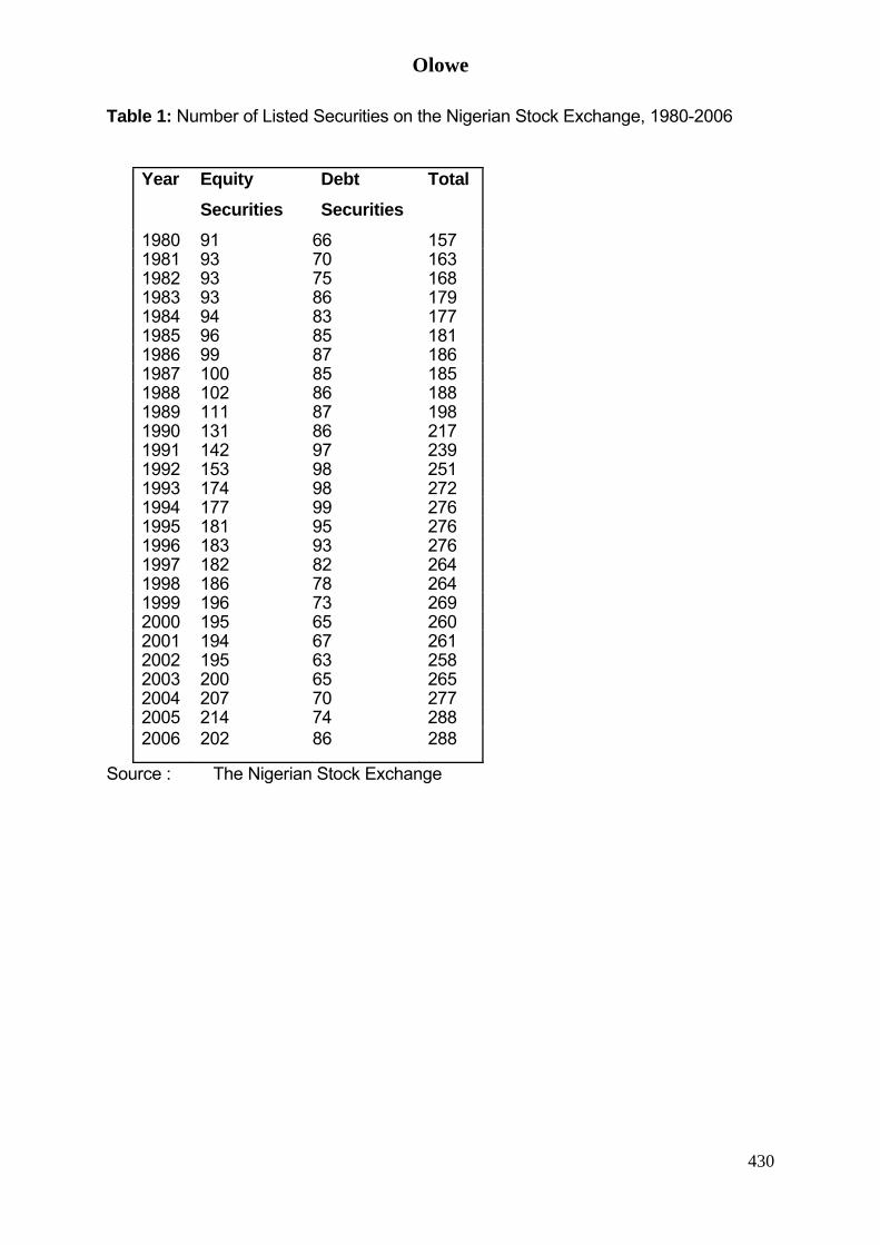
The Nigerian Stock Exchange (NSE) which started operation in 1961 with 19 securities has grown overtime. As at 1998, there are 264 securities listed on the NSE, made up of 186 equity securities and 78 debt securities (Olowe, 2008). By 2006, the number of listed securities has increased to 288 securities made up of 202 equity securities and 86 debt securities. Table 1 highlights the trends in the number of listed securities on the Nigerian Stock market. Table 2 shows the trend in the trading transactions in the Nigerian stock market. Between 1971 and 1987, there was hardly any trading transaction on the equity market. Government and industrial loan stocks dominated the transactions on the Nigerian stock market (Olowe, 2008). Table 2 shows that the value of equity traded as a proportion of total value of all securities traded, equity traded as a proportion of total market capitalisation and equity traded as a proportion of GDP are all zero between 1971 and 1987. However, since 1988 the value of equity traded transaction has been increasing in the Nigerian stock market (Olowe, 2008). Table 2 shows that equity traded as a proportion of total value of all securities traded grew from 0.7348 in 1988 to 0.9988 in 1998 and to 0.9973 in 2007. Table 2 shows that between 1988 and 2005, the equity market is still small relative to the size of the stock market. The value of equity traded as a proportion of total market capitalisation was 0.0624 in 1988 but fell to 0.0022 in 1989. Since 1989, the value of equity traded as a proportion of total market capitalisation has been fluctuating rising slightly to 0.0516 in 1998, increasing to 0.1059 in 2004 and falling to 0.0878 in 2005. On July 4, 2004, Central Bank of Nigeria o proposed banking reforms increasing the capitalisation of Nigerian banks to N25 billion. In the process of complying with the minimum capital requirement, N406.4 billion was raised by banks from the capital market, out of which N360 billion was verified and accepted by the CBN (Central Bank of Nigeria, 2005). The introduction of the 2004 bank capital requirements could have affected quoted securities on the Nigerian stock exchange. The recapitalisation of the Nigerian banking industry and influx of banking stocks into the Nigerian stock market made the value of equity traded as a proportion of total market capitalisation to increase to 81.0104 in 2007. Table 2 shows that the stock market is small relative to the size of the economy. The value of equity traded as a proportion of GDP was 0.0023 in 1988 but fell to 0.0001 in 1989. Since 1989, the value of equity traded as a proportion of GDP has been fluctuating rising slightly to 0.0033 in 1998, increasing to 0.0192 in 2004 and falling to 0.0171 in 2005. The recapitalisation of the Nigerian banking industry and influx of

Olowe

429

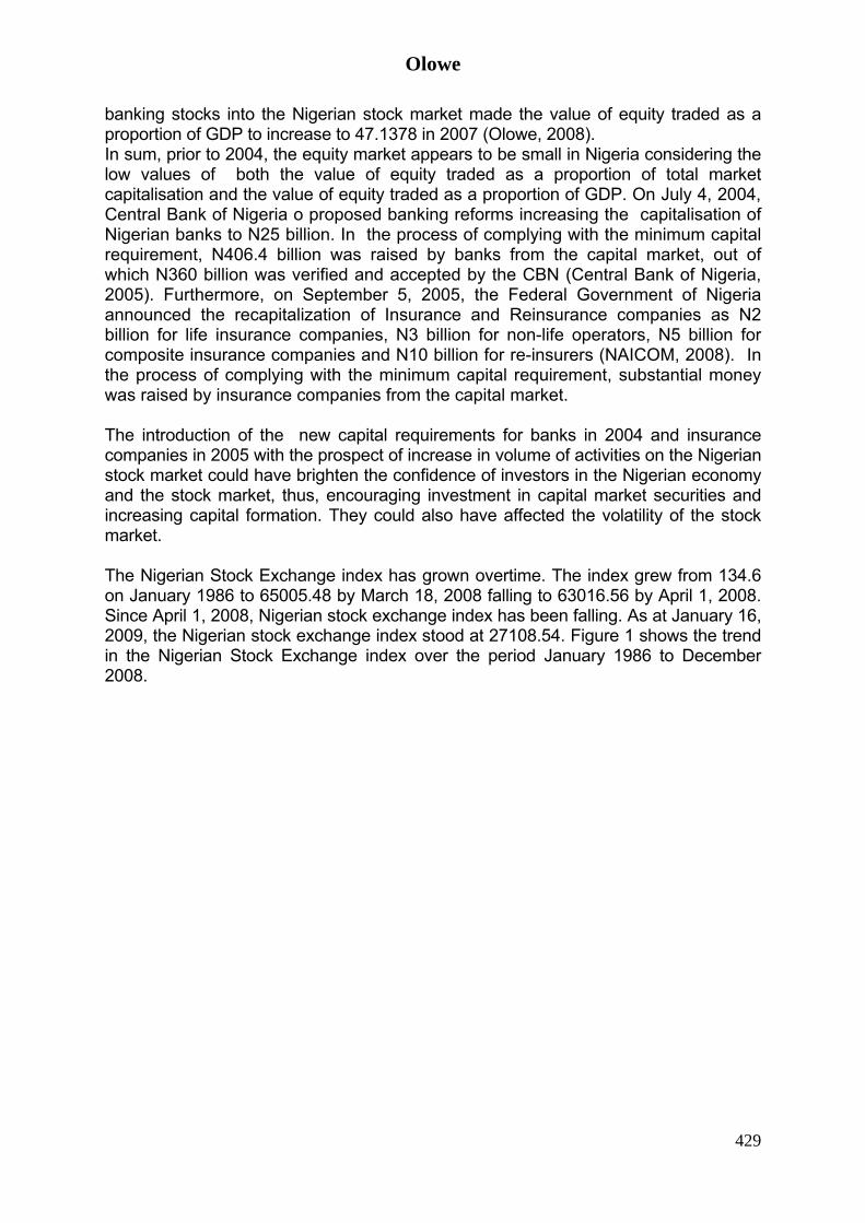
banking stocks into the Nigerian stock market made the value of equity traded as a proportion of GDP to increase to 47.1378 in 2007 (Olowe, 2008). In sum, prior to 2004, the equity market appears to be small in Nigeria considering the low values of both the value of equity traded as a proportion of total market capitalisation and the value of equity traded as a proportion of GDP. On July 4, 2004, Central Bank of Nigeria o proposed banking reforms increasing the capitalisation of Nigerian banks to N25 billion. In the process of complying with the minimum capital requirement, N406.4 billion was raised by banks from the capital market, out of which N360 billion was verified and accepted by the CBN (Central Bank of Nigeria, 2005). Furthermore, on September 5, 2005, the Federal Government of Nigeria announced the recapitalization of Insurance and Reinsurance companies as N2 billion for life insurance companies, N3 billion for non-life operators, N5 billion for composite insurance companies and N10 billion for re-insurers (NAICOM, 2008). In the process of complying with the minimum capital requirement, substantial money was raised by insurance companies from the capital market. The introduction of the new capital requirements for banks in 2004 and insurance companies in 2005 with the prospect of increase in volume of activities on the Nigerian stock market could have brighten the confidence of investors in the Nigerian economy and the stock market, thus, encouraging investment in capital market securities and increasing capital formation. They could also have affected the volatility of the stock market. The Nigerian Stock Exchange index has grown overtime. The index grew from 134.6 on January 1986 to 65005.48 by March 18, 2008 falling to 63016.56 by April 1, 2008. Since April 1, 2008, Nigerian stock exchange index has been falling. As at January 16, 2009, the Nigerian stock exchange index stood at 27108.54. Figure 1 shows the trend in the Nigerian Stock Exchange index over the period January 1986 to December 2008.

Olowe

430

Table 1: Number of Listed Securities on the Nigerian Stock Exchange, 1980-2006

Year Equity Securities

Debt Securities

Total

1980 91 66 1571981 93 70 1631982 93 75 1681983 93 86 1791984 94 83 1771985 96 85 1811986 99 87 1861987 100 85 1851988 102 86 1881989 111 87 1981990 131 86 2171991 142 97 2391992 153 98 2511993 174 98 2721994 177 99 2761995 181 95 2761996 183 93 2761997 182 82 2641998 186 78 2641999 196 73 2692000 195 65 2602001 194 67 2612002 195 63 2582003 200 65 2652004 207 70 2772005 214 74 2882006 202 86 288

Source : The Nigerian Stock Exchange

Olowe

431

Table 2: Trading Transactions on the Nigerian Stock Exchange

Year Govt. Securities and Industrial Loan

Equities Total ET/TVT ET/TMC ET/GDP

1970 16.6 - 16.6 1971 36.2 - 36.2 0 0 01972 27.2 - 27.2 0 0 01973 92.4 - 92.4 0 0 01974 50.7 - 50.7 0 0 01975 63.7 - 63.7 0 0 01976 111.9 - 111.9 0 0 01977 180 - 180 0 0 01978 189.7 - 189.7 0 0 01979 254.4 - 254.4 0 0 01980 388.7 - 388.7 0 0 01981 304.8 - 304.8 0 0 01982 215 - 215 0 0 01983 397.9 - 397.9 0 0 01984 256.5 - 256.5 0 0 01985 316.6 - 316.6 0 0 01986 497.9 - 497.9 0 0 01987 382.4 - 382.4 0 0 01988 225.5 624.8 850.3 0.7348 0.0624 0.00231989 582.4 27.9 610.3 0.0457 0.0022 0.00011990 158.5 66.9 225.4 0.2968 0.0041 0.00011991 98.7 143.4 242.1 0.5923 0.0062 0.00031992 91.7 400 491.7 0.8135 0.0128 0.00041993 348.2 456.2 804.4 0.5671 0.0096 0.00041994 192.3 793.6 985.9 0.8050 0.0120 0.00051995 50.8 1,788.00 1,838.80 0.9724 0.0099 0.00061996 62.8 6,916.80 6,979.60 0.9910 0.0242 0.00171997 107.9 10,222.60 10,330.50 0.9896 0.0363 0.00241998 15.8 13,555.30 13,571.10 0.9988 0.0516 0.00331999 0.8 14,071.20 14,072.00 0.9999 0.0469 0.00292000 8.1 28,145.00 28,153.10 0.9997 0.0596 0.00412001 35.6 57,648.20 57,683.80 0.9994 0.0870 0.00822002 2.6 59,404.10 59,406.70 0.99996 0.0777 0.00742003 6520.1 113,882.50 120,402.60 0.9458 0.0838 0.01122004 2047.5 223,772.50 225,820.00 0.9909 0.1059 0.01922005 8252.7 254683.1 262935.8 0.9686 0.0878 0.01712006 2665527.4 451597311.9 454262839.3 0.9941 88.1864 24.78202007 2870000 1,077,047,315. 1079917315. 0.9973 81.0140 47.1378

Source: Central Bank of Nigeria Annual Report and Accounts, Various issues.

Notes: ET represents value of equity securities traded. TVT represents total value of all securities traded.

TMC represents Total market capitalisation. GDP represents Gross domestic prices at current prices.

Olowe

432

Figure 1: Trend in the Nigerian Stock Exchange Index over the period, January 1986 to December, 2008

0

10000

20000

30000

40000

50000

60000

70000

86 88 90 92 94 96 98 00 02 04 06 08

Niger ian S toc k Exchang e Index

3. Literature Review The introduction of autoregressive conditional heteroskedasticity (ARCH) model by Engle (1982) as generalized (GARCH) by Bollerslev (1986) has led to the development of various models to model financial market volatility. Some of the models include IGARCH originally proposed by Engle and Bollerslev (1986), GARCH-in-Mean (GARCH-M) model introduced by Engle, Lilien and Robins (1987),the standard deviation GARCH model introduced by Taylor (1986) and Schwert (1989), the EGARCH or Exponential GARCH model proposed by Nelson (1991), TARCH or Threshold ARCH and Threshold GARCH were introduced independently by Zakoïan (1994) and Glosten, Jaganathan, and Runkle (1993), the Power ARCH model generalised by Ding,. Zhuanxin, C. W. J. Granger, and R. F. Engle (1993) among others.

Engle, Lilien and Robins (1987) introduced the GARCH-in-Mean to examine relation between stock return and volatility to enable risk-return tradeoff to be measured. Since the work of Engle, Lilien and Robins (1987), various studies have been done using the GARCH-in-Mean to explain the relation between risk and return. However, there is mixed evidence on the nature of this relationship. It has been found to be positive as well as negative (Kumar and Singh, 2008). French, Schwert and Stambaugh (1987) used daily and monthly returns on the NYSE stock index to investigate the relation between risk and return. They find evidence that expected

Olowe

433

market risk premium is positively related to predictable volatility of stock returns. Chou (1988) and Baillie and DeGennaro (1990) also found a positive relation between the predictable components of stock returns and volatility. Glosten et al. (1993) use data on the NYSE over April 1851 to December 1989, and find negative relationship between expected stock market return and volatility. However, Glosten LR, Jagannathan R, Runkle DE (1993) used the data on the New York Stock Exchange to find negative relationship between expected stock market return and volatility. Bekaert and Wu (2000) reported asymmetric volatility in the stock market and negative correlation between return and conditional volatility. There are other studies on the relation between stock return and risk using other framework other than GARCH-in-Mean model., Campbell (1987) used an instrumental variables specification for conditional moments and finds negative risk-return tradeoff . ., Pagan and Hong (1991) used non-parametric techniques and find a weak negative relationship between risk and return. Harrison and Zhang (1999) find that the relationship between risk and return is significantly positive at longer horizons. Few studies have been done on stock market volatility in emerging markets. Leon (2007) investigated the relationship between expected stock market returns and volatility in the regional stock market of the West African Economic and Monetary Union called the BRVM. Using weekly data over the period 4 January 1999 to 29 July 2005 , he found that expected stock return has a positive but not statistically significant relationship with expected volatility. He also found that volatility is higher during market booms than when market declines. Aggarwal, Inclan and Leal (1999) analyze volatility in emerging stock markets during 1985-95. They identify the points of sudden changes in the variance of returns and examine the nature of events that cause large shifts in stock return volatility in these economies. Aggarwal et al find that mostly local events cause jumps in the stock market volatility of the emerging markets. Kim and Singal (1997) and De Santis and Imorohoroglu (1994) study the behavior of stock prices following the opening of a stock market to foreigners or large foreign inflows. They find that there is no systematic effect of liberalization on stock market volatility. Hussain and Uppal (1999) examines stock returns volatility in the Pakistani equity market. He finds a strong evidence of persistence in variance in returns implying that shocks to volatility continue for a long period. However, after accounting for the structural shift due to opening of the market, the persistence was found to decline significantly. Barta (2004) examines the time variation in volatility in the Indian stock market during 1979-2003. He finds that the period around the BOP crisis and the subsequent initiation of economic reforms in India is the most volatile period in the stock market. Sudden shifts in stock return volatility in India are more likely to be a consequence of major policy changes and any further incremental policy changes may have only a benign influence on stock return volatility. 4. Methodology 4.1 The Data The time series data used in this analysis consists of daily Nigerian Stock Exchange index from January 2, 2004 to January 16, 2009 obtained from the Nigerian Stock Exchange. In this study, stock return is defined as:

Olowe

434

Rt= log1

t

t

NSINSI −

⎛ ⎞⎜ ⎟⎝ ⎠

(1)

(1) where

Rt represent stock return at time t NSIt mean Nigerian Stock Exchange index at time t NSIt-1 represent Nigerian Stock Exchange index at time t-1. The Rt of Equation (1) will be used in investigating the volatility of stock

returns in Nigeria over the period, January 2, 2004 to January 16, 2009. On July 4, 2004, the Central Bank of Nigeria, with a view to strengthening the Nigerian banking industry, announced a new capital requirement for banks operating in Nigeria. The new capitalisation of Nigerian banks was increased to N25 billion. Furthermore, on September 5, 2005, the Federal Government of Nigeria announced the recapitalization of Insurance and Reinsurance companies as N2 billion for life insurance companies, N3 billion for non-life operators, N5 billion for composite insurance companies and N10 billion for re-insurers (NAICOM, 2008). The recapitalization of the banking industry and the Insurance industry boosted the number of securities on Nigerian stock market increasing public awareness and confidence about the Stock market. This paper will investigate the impact of the banking reform (BR) and insurance reform (ISR) on the stock market volatility. To account for the banking reform in this paper, a dummy variable is set equal to 0 for the period before July 4, 2004 and 1 thereafter. To account for the insurance reform in this paper, a dummy variable is set equal to 0 for the period before September 5, 2005 and 1 thereafter. Since April 1, 2008, stock prices on the Nigerian Stock market has been declining. The stock index fell from 63016.56 on April 1, 2008 to 27108.4 on January 16, 2009. To investigate the impact of this stock market crash on stock market volatility, results will be presented separately for the period before the stock market crash (January 2, 2004- March 31, 2008) and after the stock market crash (April 1, 2008 – January 16, 2009). To account for the stock market crash (SMC) in this paper, a dummy variable is set equal to 0 for the period before April 1, 2008 and 1 thereafter. The global financial crisis of 2008 , an ongoing major financial crisis , was triggered by the subprime mortgage crisis in the United States which became prominently visible in September 2008 with the failure, merger, or conservatorship of several large United States-based financial firms exposed to packaged subprime loans and credit default swaps issued to insure these loans and their issuers (Wikipedia, 2009). On September 7, 2008, the United States government took over two United States Government sponsored enterprises Fannie Mae (Federal National Mortgage Association) and Freddie Mac (Federal Home Loan Mortgage Corporation) into conservatorship run by the United States Federal Housing Finance Agency. The two enterprises as at then owned or guaranteed about half of the U.S.'s $12 trillion mortgage market. This causes panic because almost every home mortgage lender and Wall Street bank relied on them to facilitate the mortgage market and investors worldwide owned $5.2 trillion of debt securities backed by them (Wikipedia, 2009). Later in that month Lehman Brothers and several other financial institutions failed in the United States. This crisis rapidly evolved to global crisis. In this study, September

Olowe

435

7, 2008 is taken as the date of commencement of the global financial crisis. To investigate the impact of the global financial crisis on stock market volatility, results will be presented separately for the period before the global financial crisis (January 2, 2004- September 6, 2008) and the global financial crisis period (September 7, 2008 – January 16, 2009). To account for global financial crisis (GFC) in this paper, a dummy variable is set equal to 0 for the period before September 7, 2008 and 1 thereafter.

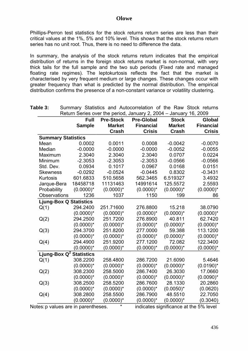
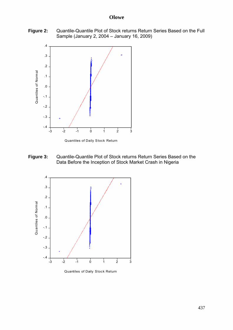
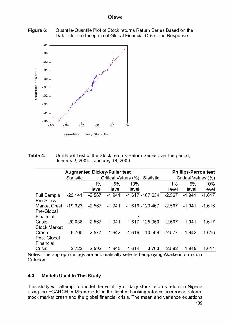
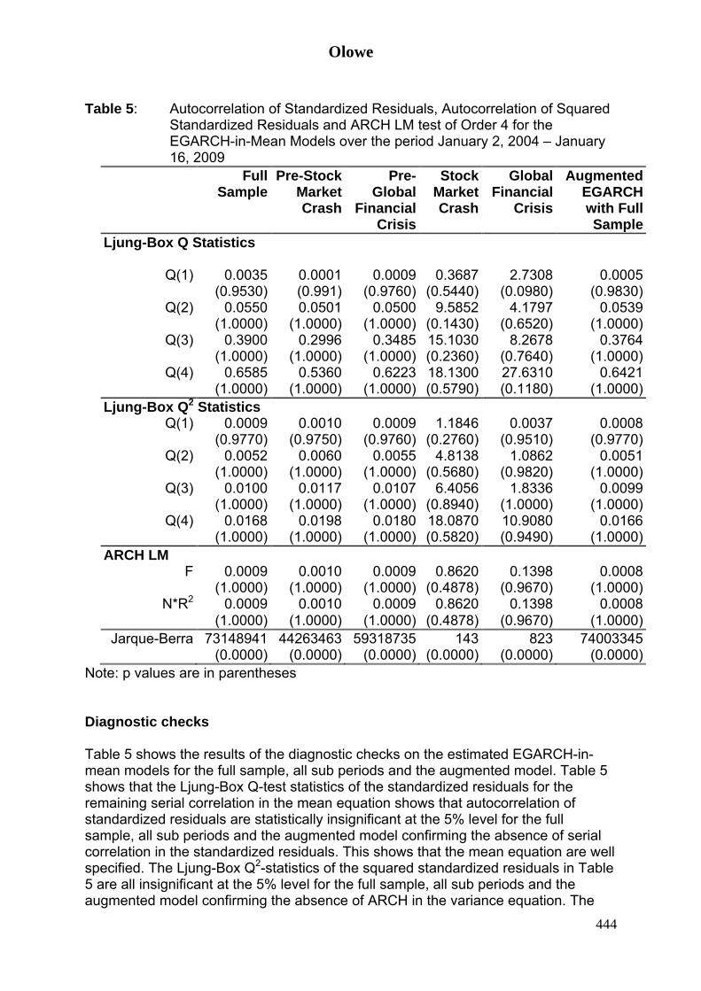
4.2 PROPERTIES OF THE DATA The summary statistics of the stock returns return series is given in Table 3. The mean return for the full sample, Pre-Stock Market Crash period, Pre-Global Financial Crisis period, Stock Market Crash period and Global Financial Crisis period are 0.0002, 0.0011, 0.0008, -0.0042 and -0.007 respectively while their standard deviations are 0.0934, 0.1017, 0.0967, 0.0168 and 0.0151 respectively. The mean return appears to be negative during Stock market crash period and global financial crisis period showing that, on average, investors sustain losses during these periods. The standard deviation appears to be lower during Stock market crash period and global financial crisis periods since returns are lower possibly reflecting positive relation between risk and return. The skewness for the full sample, Pre-Stock Market Crash period, Pre-Global Financial Crisis period, Stock Market Crash period and Global Financial Crisis period are are -0.0292, -0.0524, -0.0445, 0.8302 and -0.3431 respectively. This shows that the distribution, on average, is negatively skewed relative to the normal distribution (0 for the normal distribution). This is an indication of a non-symmetric series. The kurtosis for full sample, Pre-Stock Market Crash, Pre-Global Financial Crisis, Stock market crash period and Global Financial Crisis are very much larger than 3, the kurtosis for a normal distribution. Skewness indicates non-normality, while the relatively large kurtosis suggests that distribution of the return series is leptokurtic, signaling the necessity of a peaked distribution to describe this series. This suggests that for the stock returns return series, large market surprises of either sign are more likely to be observed, at least unconditionally. The Ljung-Box test Q statistics for the full sample, Pre-Stock Market Crash, Pre-Global Financial Crisis, Stock market crash and Global Financial Crisis periods are all significant at the 5% for all reported lags confirming the presence of autocorrelation in the stock returns return series. Jarque-Bera normality test rejects the hypothesis of normality for the full sample, Pre-Stock Market Crash, Pre-Global Financial Crisis, Stock market crash and Global Financial Crisis periods. Figures 2, 3, 4, 5 and 6 shows the quantile-quantile plots of the stock returns for the for the full sample, Pre-Stock Market Crash, Pre-Global Financial Crisis, Stock market crash period and Global Financial Crisis periods. Figures 2, 3, 4, 5 and 6 clearly show that the distribution of the stock returns return series show a strong departure from normality. The Ljung-Box test Q2 statistics for the full sample, Pre-Stock Market Crash, Pre-Global Financial Crisis, Stock market crash period and Global Financial Crisis periods are all significant at the 5% for all reported lags confirming the presence of heteroscedasticity in the stock returns return series. Table 4 shows the results of unit root test for the stock returns return series. The Augmented Dickey-Fuller test and

Olowe

436

Phillips-Perron test statistics for the stock returns return series are less than their critical values at the 1%, 5% and 10% level. This shows that the stock returns return series has no unit root. Thus, there is no need to difference the data. In summary, the analysis of the stock returns return indicates that the empirical distribution of returns in the foreign stock returns market is non-normal, with very thick tails for the full sample and the two sub periods (Fixed rate and managed floating rate regimes). The leptokurtosis reflects the fact that the market is characterised by very frequent medium or large changes. These changes occur with greater frequency than what is predicted by the normal distribution. The empirical distribution confirms the presence of a non-constant variance or volatility clustering. Table 3: Summary Statistics and Autocorrelation of the Raw Stock returns

Return Series over the period, January 2, 2004 – January 16, 2009 Full

Sample Pre-Stock

Market Crash

Pre-Global Financial

Crisis

Stock Market Crash

Global Financial

Crisis Summary Statistics Mean 0.0002 0.0011 0.0008 -0.0042 -0.0070Median -0.0000 -0.0000 -0.0000 -0.0052 -0.0055Maximum 2.3040 2.3040 2.3040 0.0707 0.0224Minimum -2.3053 -2.3053 -2.3053 -0.0566 -0.0566Std. Dev. 0.0934 0.1017 0.0967 0.0168 0.0151Skewness -0.0292 -0.0524 -0.0445 0.8302 -0.3431Kurtosis 601.6833 510.5658 562.3465 6.519327 3.4932Jarque-Bera 18458718 11131463 14991614 125.5572 2.5593Probability (0.0000)* (0.0000)* (0.0000)* (0.0000)* (0.0000)*Observations 1236 1037 1150 199 86Ljung-Box Q Statistics Q(1) 294.2400 251.71600 276.8800 15.218 38.0790 (0.0000)* (0.0000)* (0.0000)* (0.0000)* (0.0000)*Q(2) 294.2500 251.7200 276.8900 40.811 62.7420 (0.0000)* (0.0000)* (0.0000)* (0.0000)* (0.0000)*Q(3) 294.3700 251.8200 277.0000 59.388 113.1200 (0.0000)* (0.0000)* (0.0000)* (0.0000)* (0.0000)*Q(4) 294.4900 251.9200 277.1200 72.082 122.3400 (0.0000)* (0.0000)* (0.0000)* (0.0000)* (0.0000)*Ljung-Box Q2 Statistics Q(1) 308.2200 258.4800 286.7200 21.6090 5.4646 (0.0000)* (0.0000)* (0.0000)* (0.0000)* (0.0190)*Q(2) 308.2300 258.5000 286.7400 26.3030 17.0660 (0.0000)* (0.0000)* (0.0000)* (0.0000)* (0.0090)*Q(3) 308.2500 258.5200 286.7600 28.1330 20.2860 (0.0000)* (0.0000)* (0.0000)* (0.0050)* (0.0620)Q(4) 308.2800 258.5500 286.7900 48.5510 22.7050 (0.0000)* (0.0000)* (0.0000)* (0.0000)* (0.3040)

Notes: p values are in parentheses. * indicates significance at the 5% level

Olowe

437

Figure 2: Quantile-Quantile Plot of Stock returns Return Series Based on the Full Sample (January 2, 2004 – January 16, 2009)

-.4

-.3

-.2

-.1

.0

.1

.2

.3

.4

-3 -2 -1 0 1 2 3

Quantiles of Daily S tock Return

Qua

ntile

s of

Nor

mal

Figure 3: Quantile-Quantile Plot of Stock returns Return Series Based on the

Data Before the Inception of Stock Market Crash in Nigeria

-.4

-.3

-.2

-.1

.0

.1

.2

.3

.4

-3 -2 -1 0 1 2 3

Quantiles of Daily S tock Return

Qu

antil

es o

f N

orm

al

Olowe

438

Figure 4: Quantile-Quantile Plot of Stock returns Return Series Based on the Data Before the Inception of Global Financial Crisis and Response

-.4

-.3

-.2

-.1

.0

.1

.2

.3

.4

-3 -2 -1 0 1 2 3

Quantiles of Daily S tock Return

Qu

antil

es o

f N

orm

al

Figure 5: Quantile-Quantile Plot of Stock returns Return Series Based on the

Data after the Inception of Stock Market Crash in Nigeria

-.06

-.04

-.02

.00

.02

.04

.06

-.08 -.04 .00 .04 .08

Quantiles ofDaily S toc k Return

Qu

antil

es o

f N

orm

al

Olowe

439

Figure 6: Quantile-Quantile Plot of Stock returns Return Series Based on the Data after the Inception of Global Financial Crisis and Response

-.05

-.04

-.03

-.02

-.01

.00

.01

.02

.03

.04

-.06 -.04 -.02 .00 .02 .04

Quantiles of Daily Stock Return

Qu

antil

es o

f N

orm

al

Table 4: Unit Root Test of the Stock returns Return Series over the period,

January 2, 2004 – January 16, 2009

Augmented Dickey-Fuller test Phillips-Perron test Statistic Critical Values (%) Statistic Critical Values (%)

1% level

5% level

10% level

1% level

5% level

10% level

Full Sample -22.141 -2.567 -1.941 -1.617 -107.634 -2.567 -1.941 -1.617Pre-Stock Market Crash

-19.323 -2.567 -1.941 -1.616 -123.467

-2.567 -1.941 -1.616

Pre-Global Financial Crisis

-20.038 -2.567 -1.941\

-1.617 -125.950

-2.567 -1.941 -1.617Stock Market Crash

-6.705 -2.577 -1.942 -1.616 -10.509

-2.577 -1.942 -1.616

Post-Global Financial Crisis

-3.723 -2.592 -1.945 -1.614 -3.763

-2.592 -1.945 -1.614Notes: The appropriate lags are automatically selected employing Akaike information Criterion 4.3 Models Used In This Study This study will attempt to model the volatility of daily stock returns return in Nigeria using the EGARCH-in-Mean model in the light of banking reforms, insurance reform, stock market crash and the global financial crisis. The mean and variance equations

Olowe

440

that will be used for the full sample, pre-stock market crash, pre-global financial crisis, stock market crash and global financial crisis periods are given as: For the Full Sample, the mean and variance equations are given as : Rt = b0 +b1Rt-1 +b2σt +b3BR +b4ISR +b5SMC + b6GFC + εt (2)

2

t t 1 t t/ ~ N(0, , v )−ε φ σ (3)

2 2t 1 t 1t 1 t 1

t 1 t 1

2log( ) log( )− −−

− −

ε εσ = ω+α − +β σ + γ

σ π σ (4)

where vt is the degree of freedom For the pre-stock market crash period, the mean equation (2) is modified as: Rt = b0 +b1Rt-1 + b2σt +b3BR +b4ISR + εt 2

t t 1 t t/ ~ t(0, , v )−ε φ σ (5) The variance equation of the pre-stock market crash period is the same as Equation (4). For the Pre-global financial crisis, the mean equation (2) is given as: Rt = b0 +b1Rt-1 + b2σt +b3BR +b4ISR +b5SMC + εt 2

t t 1 t t/ ~ t(0, , v )−ε φ σ (6) The variance equation of the pre-global financial crisis period is the same as Equation (4). For the stock market crash period, the mean equation (2) is given as: Rt = b0 +b1Rt-1 + b2σt + b6GFC + εt 2

t t 1 t t/ ~ t(0, , v )−ε φ σ (7) The initial test of the variance equation of the stock market crash period using Equation (4) still gave the presence of ARCH in the variance equation. Thus, the variance equation of the stock market crash period is given as:

22 2t i t 1t i 1 t 1

i 1 t i t 1

2log( ) log( )− −−

= − −

ε εσ = ω+ α − +β σ + γ

σ π σ∑ (8)

The mean equation of the global financial crisis period is given as: Rt = b0 +b1Rt-1 + b2σt 2

t t 1 t t/ ~ t(0, , v )−ε φ σ (9) The variance equation used in the global financial period that achieved convergence and absence of ARCH in the variance equation is given as:

Olowe

441

22 t 1 t 1t j t j

j 1t 1 t 1

2log( ) log( )− −−

=− −

ε εσ = ω+α − + β σ + γ

σ π σ∑ (10)

To account for the shift in variance as a result of the stock market crash and global financial crisis, the full sample is re-estimated with the mean equation (2) while the variance equation is augmented as follows:

2 2t 1 t 1t 1 t 1

t 1 t 1

2log( ) log( )− −−

− −

ε εσ = ω+α − +β σ + γ

σ π σ+ Θ1SMC +Θ2GFC (11)

The volatility parameters to be estimated include ω, α, β and γ. As the stock returns return series shows a strong departure from normality, all the models will be estimated with Student t as the conditional distribution for errors. The estimation will be done in such a way as to achieve convergence. 4. The Results The results of estimating the EGARCH-in-Mean models as stated in Section 4.3 for the full sample, pre-stock market crash, pre-global financial crisis, stock market crash and global financial crisis periods are presented in Tables 4. In the mean equation, b1 (coefficient of lag of stock returns) is significant in the full sample, all sub periods and the augmented model confirming the correctness of adding the variable to correct for autocorrelation in the stock return series. The mean equation further shows that b2 (the coefficient of expected risk) is positive and insignificant in the full sample; all sub periods and the augmented model. This shows that there is little evidence on the statistical relationship between stock return and its own volatility. In other words, conditional standard deviation weakly predicts power for stock returns. The result is consistent with the work of French et al. (1987), Baillie and DeGennaro (1990), Chan et al. (1992) and Leon (2007). The coefficient b3 (coefficient of the banking reform) in the mean equation is negative and statistically significant at the 5% level as reported in the full sample, pre-stock market crash, pre-global financial crisis and the augmented model. This implies that the new bank capital requirement announced in 2004 negatively impacts on stock returns. The result of Table 3 further shows that coefficient b4 (coefficient of the insurance reform) in the mean equation is statistically insignificant at the 5% level as reported in the full sample, pre-stock market crash, pre-global financial crisis and the augmented model. This implies that the new capital requirement of insurance companies announced in 2005 has no impact on stock returns. The coefficient b5 (coefficient of stock market crash) is negative and statistically significant at the 5% level in the full sample, pre-global financial crisis and the augmented model. This shows that the stock market crash since April 2008 negatively impacts on stock returns in Nigeria. The coefficient b6 (coefficient of global financial crisis) is statistically insignificant in the full sample, stock market crash period and the augmented model implying that the global financial crisis has no impact on stock returns in Nigeria. With the exception of global financial crisis period, the variance equation in Table 4 shows that the sum of α coefficients are positive and statistically significant in the full sample, all the sub periods and the augmented model. This confirms that the ARCH

Olowe

442

effects are very pronounced implying the presence of volatility clustering. Conditional volatility tends to rise (fall) when the absolute value of the standardized residuals is larger (smaller) (Leon, 2007). Table 4 shows that the β coefficients (the determinant of the degree of persistence) are statistically significant in the full sample, all the sub periods and the augmented model. The sum of the β coefficients in the full sample, pre-stock market crash period, pre-global financial crisis period, stock market crash period , global financial crisis period and the augmented model are 0.6994, 0.5972, 0.6205, 0.6947, 0.9735 and 0.6413 respectively. This appears to show that there is a high persistence in volatility as the sum of βs are, on average, close to 1 in the full sample, pre-stock market crash period, pre-global financial crisis period, stock market crash period , global financial crisis period and the augmented model. The volatility persistence is higher in the full sample compared to the pre-stock market crash period, pre-global financial crisis period and the stock market crash period. The volatility persistence is lowest in the pre-stock market crash period. This appears to indicate that the stock market crash since April 2008 accounts for the high volatility persistence in the Nigerian stock market. The high volatility persistence in the global financial crisis period shows that the stock market is more volatile during the global financial crisis period. The stock market crash and the global financial crisis could have accounted for sudden changes in variance. The augmented EGARCH-in-Mean model where the stock market crash and global financial crisis variables are added to variance equation indicates that Θ1 (coefficient of stock market crash) is statistically significant while Θ2 is statistically insignificant. The volatility persistence in the augmented is also lower than that of the full sample. This appears to indicate that the stock market crash accounted for the sudden change in variance. With the exception of global financial crisis period, Table 4 shows that the coefficients of γ, the asymmetry and leverage effects, are negative and statistically significant at the 5% level in the full sample, Pre-Stock Market Crash, Pre-Global Financial Crisis, Stock Market Crash and the augmented models. In the global financial crisis period, γ is positive and statistically significant. The predominance negatively significance of γ in the results, appears to show that the asymmetry and leverage effects are accepted in the full sample, all sub periods and the augmented model. The leverage effect is rejected for the global financial crisis period while asymmetry effect is accepted for this period. The estimated coefficients of the degree of freedom, v are significant at the 5-percent level in full sample, all sub periods and the augmented model implying the appropriateness of student t distribution.

Olowe

443

Table 4: Parameter Estimates of the EGARCH-in-Mean Models January 2, 2004 – January 16, 2009 Full Sample Pre-Stock

Market Crash

Pre-Global Financial

Crisis

Stock Market Crash

Global Financial

Crisis

Augmented EGARCH with Full Sample

Mean Equation b0 0.0001 0.0011 0.0007 -0.0018 -0.0009 0.0003 0.0013 0.0018 0.0015 0.0010 (0.0003)* 0.0014b1 0.5291 0.4770 0.4821 0.6406 0.8521 0.5214 (0.0228)* (0.0265)* (0.0246)* (0.0491)* (0.0473)* (0.0234)*b2 0.1612 0.0900 0.1235 0.0277 0.0500 0.1624 (0.1112) (0.1986) (0.1372 (0.0811) (0.0499) (0.1362)b3 -0.0019 -0.0021 -0.0021 -0.0019 (0.0007)* (0.0007)* (0.0007)* (0.0007)*b4 0.0006 0.0007 0.0007 0.0006 (0.0005) (0.0005) (0.0005) (0.0004)b5 -0.0022 -0.0023 -0.0032 (0.0007)* (0.0007)* (0.0012)*b6 -0.0002 -0.0001 0.0002 (0.0010) (0.0008) (0.0015)Variance Equation ω -2.9811 -4.0154 -3.7199 -3.6718 -0.0457 -3.5729

(0.4620)* (0.6218)* (0.5289)* (1.0686)* (0.1016) (0.5273)*α1 0.2822 0.2091 0.2757 1.6859 -0.8225 0.2590

(0.0432)* (0.0489)* (0.0441)* (0.4961)* (0.3519)* (0.0441)*α2 -0.0652

(0.2751) γ -0.2263 -0.1554 -0.2156 0.4176 -1.5132 -0.2034

(0.0392)* (0.0476)* (0.0418)* (0.2140)* (0.4627)* (0.0420)*β1 0.6994 0.5972 0.6205 0.6947 0.4633 0.6413

(0.0485)* (0.0638)* (0.0559)* (0.0997)* (0.0069)* (0.0546)*β2 0.5102 (0.0025)*Θ1 0.3189 (0.0968)*Θ2 -0.1583 (0.1187)ν 3.1272 3.6814 3.1071 3.0040 2.2022 3.3030

(0.1855)* (0.2086)* (0.1865)* (0.8981)* (0.1395)* (0.1952)*LL 4200.7820 3611.2710 3927.5100 629.5107 300.7290 4206.4150Persistence 0.6994 0.5972 0.6205 0.6947 0.9735 0.6413AIC -6.7835 -6.9523 -6.8173 -6.2262 -6.7844 -6.7893SC -6.7337 -6.9045 -6.7689 -6.0607 -6.5275 -6.7313HQC -6.7647 -6.9342 -6.7990 -6.1593 -6.6810 -6.7675N 1236 1037 1150 199 86 1236EGARCH EGARCH(1,1) EGARCH(1,1 EGARCH(1,1) EGARCH(2,1) EGARCH(1,2) EGARCH(1,1)

Notes: Standard errors are in parentheses. * indicates significant at the 5% level. LL, AIC, SC, HQC and N are the maximum log-likelihood, Akaike information Criterion, Schwarz Criterion, Hannan-Quinn criterion and Number of observations respectively

Olowe

444

Table 5: Autocorrelation of Standardized Residuals, Autocorrelation of Squared

Standardized Residuals and ARCH LM test of Order 4 for the EGARCH-in-Mean Models over the period January 2, 2004 – January 16, 2009

Full Sample

Pre-Stock Market Crash

Pre-Global

Financial Crisis

Stock Market Crash

Global Financial

Crisis

Augmented EGARCH with Full Sample

Ljung-Box Q Statistics

Q(1) 0.0035 0.0001 0.0009 0.3687 2.7308 0.0005 (0.9530) (0.991) (0.9760) (0.5440) (0.0980) (0.9830)

Q(2) 0.0550 0.0501 0.0500 9.5852 4.1797 0.0539 (1.0000) (1.0000) (1.0000) (0.1430) (0.6520) (1.0000)

Q(3) 0.3900 0.2996 0.3485 15.1030 8.2678 0.3764 (1.0000) (1.0000) (1.0000) (0.2360) (0.7640) (1.0000)

Q(4) 0.6585 0.5360 0.6223 18.1300 27.6310 0.6421 (1.0000) (1.0000) (1.0000) (0.5790) (0.1180) (1.0000)

Ljung-Box Q2 Statistics Q(1) 0.0009 0.0010 0.0009 1.1846 0.0037 0.0008

(0.9770) (0.9750) (0.9760) (0.2760) (0.9510) (0.9770)Q(2) 0.0052 0.0060 0.0055 4.8138 1.0862 0.0051

(1.0000) (1.0000) (1.0000) (0.5680) (0.9820) (1.0000)Q(3) 0.0100 0.0117 0.0107 6.4056 1.8336 0.0099

(1.0000) (1.0000) (1.0000) (0.8940) (1.0000) (1.0000)Q(4) 0.0168 0.0198 0.0180 18.0870 10.9080 0.0166

(1.0000) (1.0000) (1.0000) (0.5820) (0.9490) (1.0000)ARCH LM

F 0.0009 0.0010 0.0009 0.8620 0.1398 0.0008 (1.0000) (1.0000) (1.0000) (0.4878) (0.9670) (1.0000)

N*R2 0.0009 0.0010 0.0009 0.8620 0.1398 0.0008 (1.0000) (1.0000) (1.0000) (0.4878) (0.9670) (1.0000)

Jarque-Berra 73148941 44263463 59318735 143 823 74003345 (0.0000) (0.0000) (0.0000) (0.0000) (0.0000) (0.0000)

Note: p values are in parentheses Diagnostic checks Table 5 shows the results of the diagnostic checks on the estimated EGARCH-in-mean models for the full sample, all sub periods and the augmented model. Table 5 shows that the Ljung-Box Q-test statistics of the standardized residuals for the remaining serial correlation in the mean equation shows that autocorrelation of standardized residuals are statistically insignificant at the 5% level for the full sample, all sub periods and the augmented model confirming the absence of serial correlation in the standardized residuals. This shows that the mean equation are well specified. The Ljung-Box Q2-statistics of the squared standardized residuals in Table 5 are all insignificant at the 5% level for the full sample, all sub periods and the augmented model confirming the absence of ARCH in the variance equation. The

Olowe

445

ARCH-LM test statistics in Table 5 for the full sample, all sub periods and the augmented model further showed that the standardized residuals did not exhibit additional ARCH effect. This shows that the variance equations are well specified in for the full sample, all sub periods and the augmented model. The Jarque-Bera statistics still shows that the standardized residuals are not normally distributed. In sum, all the models are adequate for forecasting purposes. 5. CONCLUSION This paper investigated the relation between stock returns and volatility in Nigeria using E-GARCH-in-mean model in the light of banking reforms, insurance reform, stock market crash and the global financial crisis. Volatility persistence, asymmetric properties and risk-return relationship are investigated for the Nigerian stock market It is found that the Nigerian stock market, returns show persistence in the volatility and clustering and asymmetric properties. This is similar kind of result was found for other emerging market ( Karmakar ,2005; Karmaka, 2006; Kaur ,2002; Kaur ,2004; Pandey, 2005; Leon, 2007; Kumar and Singh, 2008). The result also shows that volatility is persistent and there is leverage effect supporting the work of Nelson (1991) .The study found that little evidence on the relationship between stock returns and risk as measured by its own volatility. The study found positive but insignificant relationship between stock return and risk. This positive relationship is consistent with most asset-pricing models which postulate a positive relationship between a stock portfolio’s expected returns and volatility. However, in view of the insignificance relationship, the result is inconclusive as there might be need for research as to other risk measures. The result shows the banking reform in July 2004 and stock market crash since April 2008 negatively impacts on stock return while insurance reform and the global financial crisis have no impact on stock return. The stock market crash of 2008 is found to have contributed to the high volatility persistence in the Nigerian stock market especially during the global financial crisis period. The stock market crash is also found to have accounted for the sudden change in variance. It appears the stock market of emerging markets is integrated with the global financial market. It is suspected that the sub mortgage crisis in the United States which causes liquidity crisis could have put up pressure on foreign investors in the Nigerian and other emerging stock market to sell off their shares so as to provide the needed cash to address their financial problems. The continuous sale of shares by foreign investors causes the stock prices to fall in the Nigerian stock market. The fall in stock prices resulted in the loss of investor’s confidence leading to further decline as many banks that granted credit facilities for stock trading recall their loans. Further research work needs to be done as to the causes of stock market crash in the Nigerian stock market. There is a need for regulators in the emerging markets to evolve policy towards the stability and restoration of investor’s confidence in the Nigerian stock market. Governments should possibly aid the promotion of market makers towards warehousing shares and creating the market for securities trading.

Olowe

446

References Aggarwal, R., C. Inclan and R. Leal (1999) “Volatility in Emerging Stock Markets”,

Journal of Financial and Quantitative Analysis 34.

Baillie, R.T. and T. Bollerslev. 1989. “The message in daily stock returnss: A conditional-variance tale” Journal of Business and Economic Statistics 7, (3) pp. 297 -305.

Baillie, R.T. and T. Bollerslev. 1992. “Prediction in Dynamic models with Time Dependent Conditional Variances.” Journal of Econometrics. 52. 91-132.

Baillie, R. T. and R. P. DeGennarro. 1990. “Stock returns and volatility”, Journal of Financial and Quantitative Analysis 25, 203–214.

Batra, A. 2004. “Stock Return Volatility Patterns In India,” Working Paper No. 124, Indian Council For Research On International Economic Relations, March.

Bekaert, G. and G. Wu. 2000. “Asymmetric volatility and risk in equity markets”, Review of Financial Studies 13, 1– 42.

Bollerslev, T. 1986. “Generalized Autoregressive Conditional Hetroscedasticity.” Journal of Econometrics. 31. 307-327.

Bollerslev, T., R.Y. Chou and K.F. Kroner. 1992. “ARCH Modelling in Finance.” Journal of Econometrics. 52. 5-59.

Bollerslev, T, R. F. Engle and D. B. Nelson. 1994. “ARCH Models,” Chapter 49 in Robert F. Engle and Daniel L. McFadden (eds.), Handbook of Econometrics, Volume 4, Amsterdam: Elsevier.

Campbell J. 1987. Stock Returns and the Term Structure. Journal of Political Economy, 107, 205–251.

Chou, R. Y. 1988. “Volatility Persistence and Stock Valuations: Some Empirical Evidence Using GARCH,” Journal of Appl.ied Economics, 3, 279-294.

De Santis, Giorgio and S. Imrohoroglu. 1997. “ Stock Returns and Volatility in Emerging Financial Markets”, Journal of International Money and Finance, 16, August, 561-579.

Ding, Z. R.F. Engle and C.W.J. Granger. 1993. “Long Memory Properties of Stock Market Returns and a New Model”. Journal of Empirical Finance. 1. 83 – 106.

Engle, R. F. 1982. “Autoregressive Conditional Heteroscedasticity with Estimates of the Variance of United Kingdom Inflation.” Econometrica. 50(4). 987-1008.

Engle, R.F. and K.F. Kroner. 1995. “Multivariate Simultaneous Generalized ARCH.” Econometric Theory. 11. 1122 – 150.

Engle, R. F., D M. Lilien, and R P. Robins. 1987. “Estimating Time Varying Risk Premia in the Term Structure: The ARCH-M Model,” Econometrica, 55, 391–407.

French, K. R., Schwert, G. W and R. E. Stambaugh. 1987. Expected Stock Returns and Volatility. Journal of Financial Economics, 19, 3-29.

Glosten, L.R. R. Jagannathan and D. Runkle. 1993. “On the Relation between the Expected Value and the Volatility of the Nominal Excess Return on Stocks.” Journal of Finance. 48, 1779-1801.

Olowe

447

Husain, F. and J. Uppal. 1999. “Stock Returns Volatility in an Emerging Market: The Pakistani Evidence”, Pakistan Journal of Applied Economics, 15, No. 1 and 2, 19-40.

Karmakar, M. 2005. “Modeling Conditional Volatility of the Indian Stock Markets”, Vikalpa, 30, 3, 21–37.

Karmakar, M. 2006. “Stock Market Volatility in the Long Run, 1961–2005”, Economic and Political Weekly, May, 1796–1802.

Karolyi, G. A. 2001.“Why Stock Return Volatility Really Matters,” Paper Prepared for Inaugural Issue of Strategic Strategic Investor Relations,Institutional Investor Journals Series, February.

Kaur, H. 2002. “Stock Market Volatility in India”,. New Delhi: Deep & Deep Publications.

Kaur, H. 2004. “Time Varying Volatility in the Indian Stock Market”, Vikalpa, 29, 4 25–42.

Kim, C. M. and S. Kon. 1994. “Alternative Model of Conditional Heteroscedasticity in Stock Returns.” Journal of Business. 67. 563-98.

Kim, E.H. and V. Singal. 1997. “Opening up of Stock Markets: Lessons from Emerging Economies” Virginia Tech. Working Paper.

Kumar, B., and P. Singh. 2008. “Volatility Modeling, Seasonality and Risk-Return Relationship in GARCH-in-Mean Framework: The Case of Indian Stock and Commodity Markets,” Indian Institute Of Management Ahmedabad W.P. No.2008-04-04, April.

Lee, J.H.H. and M.L. King. 1993. “ A Locally Most Mean Powerful Based Score Test for ARCH and GARCH Regression Disturbances” Journal of Business and Economic Statistics,11, 11 - 27.

Léon, N. K. 2007. “ Stock market returns and volatility in the BRVM”, African Journal of Business Management, 15,107-112, August.

Nelson, D.B. 1991. “Conditional Heteroskedasticity in Asset Returns: A New Approach”. Econometrica, 59, 347 – 370.

Olowe, R. A. 2008. The Impact of the 1999 Regime Change from the Military to Civil Rule on the Nigerian Stock market. Unpublished paper.

Pagan, A. and Y. Hong. 1991. “Nonparametric Estimation and the Risk Premium,” In Barnett W, Powell J, Tauchen G (eds.), Nonparametric and Seminonparametric Methods in Econometrics and Statistics,Cambridge University Press, Cambridge, UK.

Pandey, A. 2005. “Volatility Models and their Performance in Indian Capital Markets”, Vikalpa, 30, 2, 27–46.

Schwert, G.W. and P.J. Seguin. 1990. “Heteroskedasticity in Stock Returns”. Journal of Finance. 4., 1129 – 1155.

Schwert, W. 1989. “Stock Volatility and Crash of ‘87,” Review of Financial Studies, 3, 77–102.

Taylor, S. 1986. “Modelling Financial Time Series” John Wiley & Sons, Great Britain. Wikipedia. 2009. “Global financial crisis of 2008–2009””, http://en.wikipedia.org, February. Zakoïan, J. M. (1994). “Threshold Heteroskedastic Models,” Journal of Economic

Dynamics and Control,18, 931-944.