Stock Market Information Production and Executive Incentives∗

Qiang Kang †

University of MiamiQiao Liu ‡

University of Hong Kong

This Draft: April 2005

AbstractWe find that an informationally efficient stock market induces firms to rely more heavilyon pay-for-performance schemes. We construct five stock market informativeness measuresusing stock trading data and analysts’ earnings forecast data. These variables, individuallyand collectively, account for the cross-sectional variation in chief executive officer (CEO) pay-performance sensitivity well. Our results are robust to the choice of estimators, samples, timeperiods, incentive measures, model specifications, and estimation methods. We also analyzethe properties of the pay-performance sensitivities of nonCEO executives and executive teams;These have similar properties as CEO pay-performance sensitivity.

JEL Classification: D80, G14, G34, J33Keywords: Market microstructure, pay-performance sensitivity, probability of informed trading,analysts’ earnings forecast

∗We appreciate comments from Ross Watts (the editor), an anonymous referee, Tim Burch, Stephen Chiu, JohnCore, Craig MacKinlay, Wing Suen, James Wang, Xianming Zhou and seminar participants at the University ofHong Kong, the University of Pennsylvania, and Hong Kong University of Science and Technology. We thank ClaraVega and Rong Qi for sharing programming code and offering computation suggestions, and Tim Burch and KaiLi for providing us with part of the data used in our empirical analysis. Financial support from the University ofHong Kong and the University of Miami (Kang) and the RGC Earmarked Research Grant HKU 7128/01H (Liu)are gratefully acknowledged. This research is also substantially supported by a grant from the University GrantsCommittee of the Hong Kong Special Administrative Region, China (Project No. AOE/H-05/99). All errors remainour own responsibility.

†Corresponding author. Mailing address: Finance Department, University of Miami, P.O. Box 248094, CoralGables, FL 33124-6552. Phone: (305)284-8286. Fax: (305)284-4800. E-mail: q.kang@miami.edu.

‡School of Economics and Finance, University of Hong Kong, Pokfulam, Hong Kong. Phone: (852)2859-1059.Fax: (852)2548-1152. E-mail: qliu@hku.hk.

Stock Market Information Production and Executive Incentives

Abstract

We predict and find empirically that an informationally efficient stock market induces

firms to rely more heavily on pay-for-performance schemes. We construct a set of

five stock market informativeness measures, on the basis of the stock trading data

and the analysts’ earnings forecast data. We find that these variables, individually and

collectively, account for the cross-sectional variations in chief executive officers’ (CEOs’)

pay-performance sensitivities well. Our results are robust to the choice of estimators,

samples, time periods, measures of incentives, model specifications, and estimation

methods. We also analyze the properties of the pay-performance sensitivities for non-

CEO executives and the executive teams. We show that they have similar properties

as CEO pay-performance sensitivity.

JEL Classification: D80, G14, G34, J33

Keywords: Market microstructure, pay-performance sensitivity, probability of informed

trading, analysts’ earnings forecast

1 Introduction

Pay-for-performance schemes have gained huge popularity in the past two decades. While

the use of stock grants, options, and other forms of equity-related incentive pay has become a

common practice, it has also been the subject of an extensive and still expanding literature.

One of the key questions of this literature is: Under what conditions will performance pay

be more effective? Put differently, under what conditions will firms rely more heavily on

pay-for-performance schemes?

Research on executive compensation and incentives has generated many useful insights.

It has been found that firm size, return volatility (risk), growth opportunity, CEO tenure (or

CEO reputation), ownership structure, industry, and time are all important determinants

of equity-based incentives.1 Our study adds to this literature by examining empirically an

important determinant of managerial incentives, the stock market informativeness, which is

suggested in Holmstrom and Tirole (1993).

Holmstrom and Tirole (1993) (HT hereinafter) analytically show that stock prices

incorporate performance information that cannot be readily extracted from the firm’s

accounting data, and that the principal can use the inferred information to design a more

effective compensation contract. That is, the more liquid the stock market is, the more

informative is the stock price, and the more effective is the performance-related pay scheme

in inducing managerial incentives. HT posits that concentrated ownership structure directly

determines market liquidity and hence managerial incentives, but this particular role of the

ownership confounds with other roles that may also affect executive incentives such as the

corporate governance channel (e.g., Hartzell and Starks, 2003).

To motivate our econometric model of the relationship between managerial incentives

1See, for example, Demsetz and Lehn (1985) and Smith and Watts (1992) for research on firm size,Garen (1994), Aggarwal and Samwick (1999), and Jin (2002) for research on return volatility (risk),Smith and Watts (1992) and Gaver and Gaver (1993) for research on growth opportunity, Bertrand andMullainathan (2001) and Milbourn (2002) for research on CEO tenure, and Ely (1991) and Murphy (1999)for research on industry and year effects. Hartzell and Starks (2003) explore how ownership, especially,institutional investors, affects managerial incentives.

1

and stock market informativeness, we build a simple model combining the optimal incentive

contracting with stock trading. Our model abstracts from the ownership structure

assumption and yields the same empirical implications as the HT model. We show

analytically that there is a positive relation between pay-performance sensitivity and stock

price informativeness.

We test the predictions using executive compensation data drawn from Compustat’s

ExecuComp database during the period 1992–2001. We focus our empirical analysis on CEO

incentives. Following the compensation literature (e.g., Jensen and Murphy, 1990; Hall and

Liebman, 1998; and Aggarwal and Samwick 1999), we estimate pay-performance sensitivity

by examining the empirical relation between changes in executive firm-related wealth and

changes in shareholder wealth. We use two metrics of pay-performance sensitivity. One

is stock-based pay-performance sensitivity (PPS), which measures the change in dollar

value of a CEO’s holdings of stocks and stock options per $1,000 increase in the firm’s

shareholder wealth. The other is total pay-performance sensitivity (PPS TOT ), which

measures the change in dollar value of a CEO’s total firm-related wealth per $1,000 increase

in the firm’s shareholder wealth. Hall and Liebman (1998) and Murphy (1999) find that the

former accounts for the majority of CEO incentives and can also be measured more precisely

compared to other compensation components. We thus mainly rely on the stock-based PPS

to interpret the empirical results.

We construct five proxies for stock market informativeness. We use the the stock trading

data to compute probability of informed trading (PIN) for each firm-year observation

(Easley, Kiefer, O’Hara, and Paperman, 1996, 1997). PIN directly estimates the amount

of information held by traders on a specific stock. We also exploit the information

contained in the analysts’ earnings forecast data to construct four other proxies for stock

market informativeness: DISPER (the standard deviation of earnings forecast scaled by

the absolute value of the mean earnings forecast), DISPERP (the standard deviation of

earnings forecast scaled by the stock price), FE (analyst earnings forecast error normalized

2

by actual earnings), and FEP (analyst earnings forecast error normalized by the stock price).

The five variables capture different aspects of stock market informativeness.

We conduct various empirical tests of the hypothesis that pay-performance sensitivity

increases with stock market informativeness. We find strong empirical support for this

hypothesis. Specifically, we find that pay-performance sensitivity is strongly and positively

related to PIN , but significantly negatively related to FE, FEP , DISPER, and

DISPERP , respectively.

All of these results are economically significant. Per $1,000 increase in the shareholder

value, the CEO pay-performance sensitivities at the 25 percentile level of the stock market

informativeness are $1.942, $1.784, $3.534, $2.481, and $5.4 smaller than the CEO pay-

performance sensitivities at the 75 percentile level of the market informativeness, if the

stock market informativeness proxies are PIN , FE, FEP , DISPER, and DISPERP ,

respectively. They represent respective reductions of 15.12%, 13.89%, 27.51%, 19.31%,

and 42.04% from the median pay-performance sensitivity in our sample. Stock market

informativeness also accounts for the cross-section differences in CEO pay-performance

sensitivities. The overall results thus strongly suggest that an informationally efficient stock

market induce firms to rely more heavily on equity-based incentives.

We include two ownership variables in all regressions. One variable captures the total

institutional holdings and the other measures the concentration of institutional holdings.

With the ownership effects controlled for, we use the five stock market informativeness

measures to find a positive relation between CEO pay-performance sensitivity and stock

market informativeness. This evidence suggests that the stock market informativeness

measures capture the effect not accounted for by ownership structure.2

We find that our results are robust to the choice of estimators, samples, time periods,

measures of incentives, model specifications, and estimation methods. We further extend

2Our results shows that ownership structure is not the only, even not the main, channel through whicha firm’s stock liquidity and stock price informativeness are affected. Our findings thus do not support themodelling assumption made in HT.

3

our analysis to non-CEO executives and the ‘executive teams’ as well.3 We find that, like

CEO pay-performance sensitivities, executive pay-performance sensitivities, individually or

in teams, are positively related to the stock market informativeness. We also find that the

impact of stock market informativeness on pay-performance sensitivity is much larger for

CEOs than for non-CEO executives.

The paper proceeds as follows. Section 2 develops the main hypothesis of the paper.

Section 3 discusses the data and the empirical method. Section 4 presents the empirical

results. Section 5 discusses additional economic and measurement issues. Section 6 extends

our empirical analysis to non-CEO executives and executive teams. Section 7 concludes.

2 Development of Hypothesis

The Holmstrom and Tirole (1993) study is one of the first papers to combine market

microstructure with compensation contract theory. HT show that the stock price

incorporates performance information that cannot be extracted from the firm’s current or

future profit data. The amount of information contained in the stock price is useful for

structuring managerial incentives. An illiquid market makes the stock price less informative

and thus reduces the benefits of stock market monitoring.

In HT, stock market acts as an external monitoring mechanism that aligns the managers’

interest with that of shareholders. In the stock market an informed party (a speculator) take

advantage of liquidity traders to disguise his private information and make money on it.

Hence, the speculator has incentives to spend resources on collecting signals about the firm’s

fundamental value. The increased information flow into the market improves the information

content of the stock price, which enable firms to design a more efficient managerial contracts.

HT show analytically that the pay-performance sensitivity of managerial compensations is

higher when the signal observed by the speculator is more precise or the amount of liquidity

3We thank the referee for making this suggestion to us.

4

trade is larger. (See Proposition 3 in HT). That is, the information content of stock price is

positively related to the pay-performance sensitivity.

HT pinpoint the importance of the market microstructure aspect in inducing executive

incentives. However, this aspect has not been rigorously tested in the literature partly

because it is difficult to build an empirical analysis based on HT. To better motivate

the empirical analysis of the relation between stock market informativeness and executive

compensation, we propose in the Appendix an alternative one-period model which combines

the optimal contracting with stock trading. In contrast with HT which assumes that

ownership structure determines market liquidity endogenously, we assume that the market

liquidity is exogenously given. This modeling choice, although yields the same empirical

implications as those in HT, allows us to clearly control for the monitoring effect of

ownership structure, and focus on examining how stock price informativeness affects the

pay-performance sensitivity.

The key insights of our model, immediately from Propositions 2-3 in the Appendix, can

be summarized as follows:

Main results: (1) The pay-performance sensitivity decreases with the manager’s effort

parameter, the degree of risk aversion, and increases with the degree of stock price

informativeness. (2) The stock market informativeness increases with the number of informed

traders which is determined by various market microstructure parameters, e.g., the cost of

collecting information, market liquidity, uncertainty of the stock value, etc.

The key prediction from our model is consistent with the key prediction from HT. That

is, the more informative the stock price is, the more effective is the compensation scheme in

inducing managers’ incentives. The core hypothesis for our empirical study is:

H1: The pay-performance sensitivity increases with stock market informativeness.

5

3 Data and Empirical Method

Our primary data set for executive compensation is the ExecuComp database from 1992

through 2001. The database reports annual compensation flows as well as information related

to changes in the value of stock and stock option holdings for five most-paid executives,

including the CEO, for each firm appearing in the S&P500 Index, S&P mid-cap 400 Index,

and the S&P small-cap 600 Index. We obtain stock return data from the CRSP Monthly

Stock File and accounting information from the Compustat Annual File. We use five proxies

to measure the stock market informativeness and construct them from two databases. We

compute a firm’s probability of informed trading (PIN) in a given year by using intraday

trading data extracted from the TAQ database. We calculate four other variables by using

analysts’ earnings forecast information retrieved from the I/B/E/S History Summary File.

We obtain institutional equity holdings from the CDA Spectrum database, which derives

these holdings from institutional investors’ 13-f filings.

For our empirical study, we construct a sample containing 2,507 publicly traded firms

and 17,584 CEO-firm-year observations. All monetary terms are in 1992 constant dollars.

To remove the inflation effect from the empirical study, we adjust nominal stock returns with

CPI to obtain returns in real terms.

3.1 Measuring CEO Incentives

Because the CEO makes most major corporate decisions and exerts the greatest influence on

the firm among senior executives, we focus on incentive provisions for CEOs.4 We measure

incentive by the pay-performance sensitivity, which is defined as the dollar value change

in the CEO’s firm-specific wealth per $1,000 change in the shareholder value (Jensen and

Murphy, 1990).

4We extend our empirical analysis to non-CEO executives and executive teams in Section 6. We identifyCEOs by the fields “BECAMECE” and “CEOANN”. Using only “CEOANN” is problematic, since there aremany missing observations for the earlier periods of the sample (Milbourn, 2002).

6

CEO compensation comprises several different layers. Total current compensation (TCC)

is the sum of salary and bonus. Total direct compensation (TDC) is the sum of total current

compensation, other annual short-term compensation, payouts from long-term incentive

plans, the Black-Scholes (1973) value of stock options granted, the value of restricted stocks

granted, and all other long-term compensation. Both TCC and TDC measure the direct

payment a CEO receives from his firm within one fiscal year. However, neither TCC nor

TDC considers the indirect compensation that a CEO derives from a revaluation of stocks

and stock options already granted to him in previous years.

We compute the change in value of a CEO’s stock holdings over a given year as the

beginning-of-year value of his stock holdings multiplied by this year’s stock return. It

is important to revalue the stock option portfolios. ExecuComp contains the values of

unexercised exercisable and unexercisable in-the-money options, but the database measures

only the intrinsic value of the option portfolios. We apply the Black-Scholes (1973) model to

revalue the stock option portfolios. We adopt the Core and Guay’s (1999) method to compute

the hedge ratio delta (δ) of each option.5 Delta refers to how the value of a stock option varies

given a one-dollar change in the value of the underlying stock.6 We then multiply the option

deltas by the change in the firm’s market value (or change in shareholders’ wealth), adjusting

for the percentage of stock shares represented by the options, and then add the value from

stock option exercise to obtain the change in value of the CEO’s option holdings. The change

in CEO’s total firm-specific wealth (DTOTW ) is the sum of the direct compensation and

the indirect compensation due to the revaluation of stocks and stock option holdings.

We define the change in shareholder value (V CHANGE) over a given year as the

firm’s beginning-of-year market value times the year’s stock return. Using V CHANGE

5Core and Guay’s (1999) method quite accurately accounts for the economically meaningful value of thein-the-money options, but their method ignores the value of out-of-the-money options. This may likely createsystematic bias for firms with more underwater options and for firms with options that are at-the-money ornear-the-money. This concern is partially alleviated since our results are robust to the subperiod analysis inSection 5.2 where the sample is divided into the bubble period and the post-bubble period.

6For simplicity, some researchers use 0.7 as the δ value.

7

and DTOTW , we calculate PPS TOT as the dollar value change in the CEO’s total firm-

related wealth per $1,000 change in the shareholder value.

We define the stock-based pay-performance sensitivity (PPS) as the change in dollar

value of the CEO’s existing stock-based compensation (stocks and stock options) for a

$1,000 change in the shareholders’ wealth. We can interpret the stock-based pay-performance

sensitivity as the CEO’s stock ownership plus incentives from stock option holdings. Using

the option delta (δ) we obtain:

PPSit = (SHROWNPCit−1 +(Number of Options Held)it−1

(Number of Shares Outstanding)it−1

δ) ∗ 1000, (1)

where SHROWNPC is the CEO’s ownership percentage.

PPS is more appealing than PPS TOT for our empirical analysis. We can estimate

the revaluations of existing stock and stock options with relative precision compared to

measuring the impact of firm performance on the changes in total direct compensation.

Including grants of stock options and restricted stocks can be problematic, because they

might serve as an ex-post bonus mechanism rather than an ex-ante incentive mechanism.

We therefore, focus primarily on the stock-based incentives. The analysis using PPS TOT ,

which we include as a robustness check, yields essentially the same results.

Panel A of Table 1 presents the summary statistics of the CEO’s compensation

and incentive measures. For the average (median) CEO in our sample, total current

compensation (TCC) is $960,776 ($680,813) in 1992 constant dollars. Total direct

compensation (TDC) ranges from zero to $564.17 million, with an average value of $3.3

million and a median value of $1.42 million. An average (median) CEO holds 3.33% (0.43%)

of his firm’s stocks. A CEO gains an average of $1.92 million from stock option revaluation

with a standard deviation of $34.86 million. The median option revaluation is worth $0.21

million. Overall, the change of the CEO’s total firm-related wealth (DTOTW ) has a mean

value of $18.83 million and a median value of $2.3 million. We note that every compensation

8

measure, particularly DTOTW , is highly right-skewed. The annual change in shareholders’

value (VCHANGE) has a mean of $457.17 million, and a median of $61.79 million.

The mean and median values of the stock-based incentive measure (PPS), as defined

in equation (2), are respectively, $40.79 and $12.85, respectively, per $1,000 change in the

shareholders’ value. The PPS measure has a standard deviation of $74.59 with a maximum

value of $994.45. The total pay-performance sensitivity (PPS TOT ) has a mean of $46.51,

which is higher than PPS, but it also has a slightly larger standard deviation ($81.92). The

median of PPS TOT is $13.09 and is almost the same as the median of PPS. The stock-

based incentive does not deviate much from the total incentive, corroborating the findings

in prior studies that changes in the value of stock and stock option holdings account for the

majority of pay-performance sensitivities (Hall and Liebman, 1998; and Murphy, 1999).

Panel A of Table 1 also reports the summary statistics of pay-performance sensitivity

for all executives, and the executive teams. We compute PPS EXE based on equation (2)

for all five most-paid executives within a firm (including the CEO). PPS EXE measures

the stock-based incentive of an individual executive. We obtain PPS TEAM by summing

up PPS EXE across all five most-paid executives within a firm. PPS TEAM captures

the executive team’s incentives. The mean and median values of PPS EXE are $15.76 and

$2.75, respectively, both of which are significantly smaller than those of CEO incentives.

The mean (median) of PPS TEAM is $64.41 ($24.25), and the majority of team incentives

is attributable to the CEO incentives.

3.2 Measuring Stock Market Informativeness

3.2.1 Probability of Informed Trading (PIN)

Easley, Kiefer, O’Hara, and Paperman (1996, 1997) develop and use the PIN variable to

measure the probability of informed trading in the stock market. The measure is based on

the market microstructure model introduced in Easley and O’Hara (1992), where trades can

9

come from liquidity traders or from informed traders. The literature has firmly established

the PIN variable as a good measure of stock price informativeness in various settings.7

PIN directly estimates the amount of information held by traders on a specific stock, and

it is a good empirical variable to test our hypothesis that stock prices have an active role in

enhancing pay-performance sensitivity.

Our description of the model and how we construct the PIN measure are as follows.

There are three types of players in the game, liquidity traders, informed traders, and market

makers. The arrival rate of liquidity traders who submit buy orders (or sell order) is ε. Every

day, the probability that an information event occurs is α, in which case the probability of

bad news is δ and the probability of good news is (1 − δ). If an information event occurs,

the arrival rate of informed traders is µ. Informed traders submit a sell order if they get bad

news and a buy order if they get good news. Thus, on a day without information events,

which occurs with probability (1−α), the arrival rate of a buy order will be ε and the arrival

rate of a sell order will be ε as well. On a day with a bad information event (with probability

αδ), the arrival rate of a buy order will be ε and the arrival rate of a sell order will be ε + µ.

On a day with a good information event (with probability α(1 − δ)), the arrival rate of a

buy order will be ε + µ and the arrival rate of a sell order will be ε. The likelihood function

for a single trading day is:

L(θ|B, S) = (1− α)e−ε (ε)B

B!e−ε (ε)

S

S!+ αδe−ε (ε)

B

B!e−ε+µ (ε + µ)S

S!

+α(1− δ)e−ε+µ (ε + µ)B

B!e−ε (ε)

S

S!, (2)

where θ = (ε, α, δ, µ), B is the number of buy orders, and S is the number of sell orders in

a single trading day. We infer trade direction from intraday data based on the algorithm

proposed in Lee and Ready (1991).

7See, e.g., Easley, O’Hara, and Srinivas (1998); Easley, Hvidkjaer, and O’Hara (2002); Chen, Goldstein,and Jiang (2003); and Vega (2004).

10

Using the number of buy and sell orders in every trading day within a given year,

M = (Bt, St)Tt=1, and assuming cross-trading day independence,8 we estimate the parameters

of the model (ε, α, δ, µ) by maximizing the following likelihood function:

L(θ|M) =t=T∏t=1

L(θ|Bt, St). (3)

Then, we calculate PIN by dividing the estimated arrival rate of informed trades by the

estimated arrival rate of all trades:

PIN =αµ

αµ + 2ε. (4)

We maximize the likelihood function in equation (4) for the parameter space θ and then

calculate PIN for the period 1993-2001. There are 8,456 firm-year observations after we

merge the TAQ database with the ExecuComp database.

Panel A of Table 2 presents summary statistics of PIN . In our sample, the average

PIN is 0.163 with a standard deviation of 0.051. The median value of PIN is 0.157. The

maximum PIN is 0.797 with a minimum of zero. The average sample property of our

PIN estimates is consistent with the sample proprety identified in previous studies (see, e.g,

Easley, Hvidkjaer, and O’Hara, 2002).

3.2.2 Measures Based on the Analysts’ Forecast Data

Information-based trading can only be inferred by econometricians. We supplement the

PIN measure with four other variables using the analysts’ earnings forecast data from the

I/B/E/S History Summary File. For each firm in the ExecuComp database, we use the

summary information on analysts’ fiscal year 1 earnings estimates in the ninth month of a

8This assumption is critical for estimating the model. However, Barclay and Warner (1993) find thatinformed traders engages in stealth trading. That is, they tend to camouflage their private information andspread trades over time. Therefore, the cross-trading day independence is unlikely to be satisfied. We thankthe referee for pointing this out. As shown in Section 5.3, the impact of stealth trading on our results arelikely negligible.

11

fiscal year as the raw measure.9

We compute FE as the absolute value of the difference between mean earnings forecast

and actual earnings, divided by the absolute value of actual earnings. We calculate FEP

as the absolute value of the difference between mean earnings forecast and actual earnings,

scaled by the year-end stock price. When a firm’s information production process is intense

and effective, analysts following the firm’s stock are more likely to agree with one another

on the firm’s earnings prospect. Both FE and FEP measure the intensity of a firm’s

information production. They serve as good proxies for the stock price informativeness.

We merge I/B/E/S/ with ExecuComp and delete the observations with zero actual

earnings (FE would be undefined otherwise). This results in a sample of 9,420 firm-year

observations over the period 1992-2001. Panel A of Table 2 presents summary statistics for

FE. It has a mean (median) of 0.444 (0.066) and a standard deviation of 5.014. When we

merger I/B/E/S with ExecuComp and delete the observations with zero year end stock price

(FEP would be undefined otherwise), we obtain a sample with 9,421 firm-year observations.

The mean and median values of FEP are 0.013 and 0.002 respectively. Its standard deviation

is 0.093. We note that both FE and FEP are fat-tailed and extremely right-skewed.

Akinkya and Gift (1985), Diether, Malloy, and Scherbina (2002), and Johnson (2004)

show that the dispersions of analysts’ earnings forecasts is a proxy for the information

environment in which various investors trade. A larger analyst forecast dispersion implies

less intensive information production or a less transparent information environment and vice

versa. We define DISPER as the standard deviation of earnings forecasts scaled by the

absolute value of the mean earnings forecast and times 100. If the mean earnings forecast

is zero, we exclude the stock from the sample. Combining I/B/E/S/ with ExecuComp and

deleting the observations with zero mean earnings forecast, we obtain a sample of 9,161 firm-

year observations for the period 1992-2001. Panel A of Table 2 presents summary statistics

9We also conduct the analysis by using summary information on each of the other months’ fiscal year1 earnings estimates within that fiscal year. The summary information is stable across months and is veryclose to the annual average value. Results are qualitatively similar and are not reported for brevity.

12

of DISPER. Its mean (median) is 12.116 (3.175) and its standard deviation is 66.754.

We define DISPERP as the standard deviation of earnings forecasts scaled by the year-

end stock price and times 100. Its mean and median are 0.412 and 0.135 respectively. It

has a standard deviation of 2.098. Both DISPER and DISPERP are fat-tailed and highly

right-skewed.

Panel B of Table 2 presents the bivariate Pearson correlation coefficients and their

significance levels of the five market informativeness variables. After merging the five

variables, the number of observations drops to 4,503. In this sample, the correlation between

PIN and FE is 0.019 and is not significant. The correlation between PIN and FEP

however is significant at 0.068. The correlation between PIN and DISPER is 0.04 and

is significant at the 1% level. Its correlation with DISPERP is also positively significant

at the 1% level. FE are not significantly correlated with either DISPER or DISPERP ,

although it is correlated with FEP at the 1% level. FEP is significantly correlated with

both DISPER and DISPERP at the 1% level. The piecewise correlations among the five

market informativeness proxies show similar properties, and are not reported for brevity.

Overall, our results suggest that the five variables capture different aspects of a firm’s

stock market informativeness. PIN , as argued in Easley et al. (2002), is more likely

to capture the amount of private information contained in the stock price, while the

four measures based on the analysts’ forecast data might reflect both private and public

information. However, such a distinction is only suggestive. We defer a detailed discussion

of how these variables interact with each other in our context in Section 4.3.

3.3 Control Variables

Panel B of Table 1 summarizes the control variables we use in our empirical analysis. We

obtain stock return data from CRSP. We calculate the market value (MKTV AL) at each

year-end. Our sample comprises a range of firms with an average market capitalization of

13

$4.29 billion and a median of $0.86 billion. The smallest firm has only $6,100 in market

capitalization and the largest one has $427.22 billion. We use the log value of market

capitalization (SIZE) as one measure of firm size. The mean (median) value of SIZE

is 6.91 (6.76) with a standard deviation of 1.6. The firm’s annualized percentage stock

return (ANNRET ) averages 22.45% with a median of 11.54%. The annualized percentage

volatility of stock returns (ANNV OL), which we compute by using the past five years of

monthly stock returns, has a mean value of 39.44% and a median value of 35.23%. We extract

firm-specific accounting data from Compustat. To measure a firm’s growth opportunities,

we calculate Tobin’s q as the ratio of the market value of assets to the book value of assets.10

Table 1 shows that the average Tobin’s q of the firms in our sample is 2.16. Its standard

deviation and median are 2.75, and 1.48, respectively.

We construct two institutional ownership variables to control for the monitoring effect

suggested in Harzell and Starks (2003), and to test the assumption made in the HT model

— the market informativeness relates to pay-performance sensitivity through ownership

structure. We define INSTHOLD as the total institutional share holdings as a percent of

the total number of shares outstanding. In HT, INSTHOLD should be negatively related

to market liquidity and pay-performance sensitivity. We expect institutional investors to

have greater influence if the shares are concentrated on the hands of the larger investors.

As in Hartzell and Starks (2003), we use the concentration of institutional ownership as a

proxy for institutional influence. We define INSTCON as the proportion of institutional

investor ownership accounted for by the top ten institutional investors in the firm. As shown

in Panel B of Table 1, on average, 56.47% of a firm’s shares are owned by the institutional

investors, and 60.07% of shares held by the institutional investors are controlled by the top

ten institutional investors.

Other control variables are CEO tenure, industry dummies, and year dummies. We

10We obtain the market value of assets as the book value of assets (data 6) plus the market value ofcommon equity (data 25 times data 199) less the book value of common equity (data 60) and balance sheetdeferred taxes (data 74).

14

calculate CEO tenure as the number of years the executive has been the CEO of the firm

as of the compensation year in ExecuComp. The mean and median of the CEO tenure are

7.68 and 5.5 years, respectively. The maximum tenure in our sample is 54.92 years. Finally,

we construct 20 industry dummies based on the 2-digit SIC code from CRSP.

3.4 Econometric Specifications

There are two basic econometric methods in empirical studies of incentives. One is to directly

regress the incentive measure against a set of explanatory variables. This approach makes

the regression results immediately interpretable. It also provides the flexibility to control for

factors that may affect the pay-performance sensitivity. Following this approach, we specify

the basic model as:

PPSi,t = γ0 + γ1INFOVi,t−1 + γ2sizei,t−1 + γ3annvoli,t−1 + γ4Tobinqi,t−1 + γ5tenurei,t

+γ6INSTHOLDi,t−1 + γ7INSTCONi,t−1 +∑k≥8

γkdummiesi,t + εi,t, (5)

where PPS refers to the computed pay-performance sensitivity as specified in equation (2);

INFOV stands for the set of market informativeness variables, i.e., PIN , FE, FEP ,

DISPER, and DISPERP ; and dummies are industry dummies and year dummies.

In equation (6), we control for several empirically relevant variables: firm size, return

volatility, growth opportunities, CEO tenure, industry effects, year effects, and most

importantly, institutional ownership. The coefficient γ1 captures the influence of market

informativeness on incentives and is our main parameter. We test our hypothesis by

examining the sign and significance of the estimated γ1.

Another specification, adopted in Jensen and Murphy (1990), and Aggarwal and

Samwick (1999), among others, uses the CEO’s compensation level as the dependent variable.

15

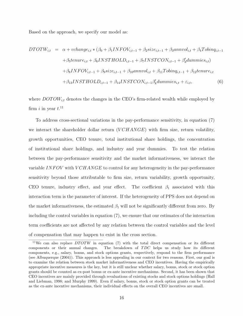
Based on the approach, we specify our model as:

DTOTWi,t = α + vchangei,t ∗ (β0 + β1INFOVi,t−1 + β2sizei,t−1 + β3annvoli,t + β4Tobinqi,t−1

+β5tenurei,t + β6INSTHOLDi,t−1 + β7INSTCONi,t−1 + β′ddummiesi,t)

+β8INFOVi,t−1 + β9sizei,t−1 + β10annvoli,t + β11Tobinqi,t−1 + β12tenurei,t

+β13INSTHOLDi,t−1 + β14INSTCONi,t−1β′kdummiesi,t + εi,t, (6)

where DOTOWi,t denotes the changes in the CEO’s firm-related wealth while employed by

firm i in year t.11

To address cross-sectional variations in the pay-performance sensitivity, in equation (7)

we interact the shareholder dollar return (V CHANGE) with firm size, return volatility,

growth opportunities, CEO tenure, total institutional share holdings, the concentration

of institutional share holdings, and industry and year dummies. To test the relation

between the pay-performance sensitivity and the market informativeness, we interact the

variable INFOV with V CHANGE to control for any heterogeneity in the pay-performance

sensitivity beyond those attributable to firm size, return variability, growth opportunity,

CEO tenure, industry effect, and year effect. The coefficient β1 associated with this

interaction term is the parameter of interest. If the heterogeneity of PPS does not depend on

the market informativeness, the estimated β1 will not be significantly different from zero. By

including the control variables in equation (7), we ensure that our estimates of the interaction

term coefficients are not affected by any relation between the control variables and the level

of compensation that may happen to exist in the cross section.

11We can also replace DTOTW in equation (7) with the total direct compensation or its differentcomponents or their annual changes. The breakdown of TDC helps us study how its differentcomponents, e.g., salary, bonus, and stock options grants, respectively, respond to the firm performance(see Albuquerque (2004)). This approach is less appealing in our context for two reasons. First, our goal isto examine the relation between stock market informativeness and CEO incentives. Having the empiricallyappropriate incentive measures is the key, but it is still unclear whether salary, bonus, stock or stock optiongrants should be counted as ex-post bonus or ex-ante incentive mechanisms. Second, it has been shown thatCEO incentives are mainly provided through revaluations of existing stocks and stock options holdings (Halland Liebman, 1998; and Murphy 1999). Even if salary, bonus, stock or stock option grants can be treatedas the ex-ante incentive mechanisms, their individual effects on the overall CEO incentives are small.

16

3.5 Testable Hypotheses and Estimation Methods

As noted earlier, the five INFOV variables, PIN , FE, FEP and DISPER, and

DISPERP , capture the market informativeness from different perspectives. A larger

value of PIN corresponds to a more informative market, and a larger value of FE, FEP ,

DISPER, or DISPERP corresponds to a less informative market. The testing of our core

hypothesis comprises several hypothesis tests, depending on which INFOV variable and

which econometric specification is used. Specifically, with the first econometric specification

in equation (6), we have

H0’: γ1 = 0, versus

H1’: γ1 > 0 if the INFOV variable is PIN ; or versus

H1”: γ1 < 0 if the INFOV variable is FE, FEP , DISPER, or DISPERP .

We replace γ1 in the above hypotheses with β1 if we use the second econometric

specification (7).

Given the apparent right skewness in the CEO compensation and incentive data (as

shown in Table 1), we follow the literature and estimate median regressions to control for

the possible influence of outliers.12 We obtain standard errors of the estimates by using

bootstrapping methods.

As a robustness check, we replace each raw measure of the five market informativeness

proxies with its cumulative distribution function (CDF) in both model specifications. As

Aggarwal and Samwick (1999) argue, the use of CDF helps to make the highly non-

homogeneous data homogeneous and the regression results economically sensible. It is

easier to transform the estimated coefficient values into pay-performance sensitivities at

any percentile of the distribution of the proxies. Thus, the CDFs give the regression results

more immediate economic intuition than the raw measures.12Most recent studies of executive compensation, e.g., Aggarwal and Samwick (1999) and Jin (2002), use

the median regression approach to deal with the apparent right skewness in the CEO compensation andincentive data.

17

4 Empirical Results

4.1 Using PPS as the Dependent Variable

Our main empirical results are based on the econometric specification in equation (6),

where we use CEO incentive measure as the dependent variable. Table 3 presents the

median regression results of the stock-based pay-performance sensitivity PPS, defined in

equation (2), by using the raw measures of the five stock market informativeness proxies. In

all regressions we control for firm size, return volatility, growth opportunity, CEO tenure,

total institutional holdings, the concentration of institutional holdings, industry dummy, and

year dummy. For brevity we do not report coefficient estimates for the industry and year

dummies.

Columns 1 shows how the CEO’s incentives respond to the probability of informed trading

(PIN). The estimated coefficients of the PIN measure (γ1) is positive and statistically

significant at the 1% significance level. γ1 is 25.284 in Column 1. The difference in PPS

between any two PIN levels is calculated as the difference in the two PIN values multiplied

by γ1. For example, because the maximum, median, and minimum PIN are 0.797, 0.157, and

0, respectively, the pay-performance sensitivity at the maximum PIN is $16.18 higher than

that at the median PIN as a result of $1,000 increase in shareholder value, all else equal. The

incentive with the median PIN is $3.97 larger than the incentive with the minimum PIN .

The economic magnitude of PIN on pay-performance sensitivity is significant, considering

that the mean (median) stock-based pay-performance sensitivity in our sample is $40.787

($12.845).

Columns 2-5 show the median regression results of using FE, FEP , DISPER, and

DISERP , respectively. γ1 in all the four regressions are negative and statistically significant

(except for FE), indicating that a less informationally efficient market leads to a lower level

of CEO incentives. Since all of the four variables are fat-tailed and right skewed, we do not

discuss their economic significance now. We defer the discussion to later regressions, when

18

the CDF transformations of these variables are used as proxies for market informativeness.

Table 3 also shows that the estimated coefficients of all of the control variables are

statistically significant and consistent in both sign and magnitude across all five regressions.

The coefficient of the lagged SIZE, γ2, is around -2.81 to -2.45, reaffirming that the pay-

performance sensitivity is negatively and strongly correlated with firm size. The coefficient

of ANNV OL, γ3, ranges from 6.61 to 18.09, implying a positive risk-incentive relation. Our

results are consistent with the model prediction of Prendergast (2002) as well as the empirical

evidence in Core and Guay (2002). However, we note that the empirical evidence on the

risk-incentive relation is mixed, and the economic rationale is still subject to a heated debate

(see the survey in Prendergast (2002)).

The coefficient of the lagged Tobinq, γ4, is about 1.49 to 1.87. There is a clearly positive

relation between growth opportunities and CEO incentives, corroborating the evidence

reported in Smith and Watts (1992) and consistent with the hypothesis that a higher

incentive level is needed when CEO effort becomes more valuable. There is also a positive

relation between CEO tenure and PPS as the estimated coefficient of tenure is approximately

0.99 to 1.37.

Notably, the coefficient of the total share holdings by institutional investors INSTHOLD

is significantly negative at -0.189 to -0.088, which seems to support the argument in HT that

a higher level of insider ownership reduces market liquidity and as a consequence, the pay-

performance sensitivity. The coefficient of the concentration of institutional share holdings

INSTCON is however significantly positive, and ranges from 0.035 to 0.154. This result

is consistent with the finding in Hartzell and Starks (2003), and suggest that institutional

influence enhance the pay-performance sensitivity.13

13We note that the two institutional variables only serve as control variables in our analysis. The additionof institutional variables does not change the signs and levels of significance of the five stock marketinformativeness measures suggests (1) The PPS – market informativeness relation is unlikely to be drivenby the ‘ownership – market liquidity’ channel proposed in HT. (2) Institutional investors’ monitoring effortdoes enhance PPS, but it seems to be an independent channel. That is, institutional investor variables playroles different from the market informativeness measures.

19

Our proxies for stock market informativeness are all fat-tailed and right skewed. A

CDF transformation of the raw measures yields more homogenous data and economically

meaningful results. Table 4 reports the results when we use the CDFs of the raw measurs

as procies for the market informativeness. The estimate coefficients of the information

variables (γ1) are 3.883, -3.568, -7.067, -4.961, and -10.799, respectively, when their respective

information variables are the CDFs of PIN , FE, FEP , DISPER, and DISPERP . All of

them are statistically significant, and have the signs consistent with our hypothesis.

The economic significance of the result is large. The pay-performance sensitivities

estimated at the 25% level of stock market informativeness are 1.942, 1.784, 3.534, 2.481, and

5.4 smaller than those estimated at the 75% level of market informativeness, representing

respective reductions of 15.12%, 13.89%, 27.51%, 19.31%, and 42.04% of median pay-

performance sensitivity in our sample.

The estimated coefficients of control variables are all statistically significant and have

magnitudes similar to those in Table 3.

The above results provide support for our conjecture that the stock market

informativeness positively affects the pay-performance sensitivity. Because we clearly

control for institutional investor variables in all of the regressions, we conclude that the

stock market informativeness and ownership structure influence pay-performance sensitivity

differently. Ownership structure is more likely to influence pay-performance sensitivity

through monitoring channel. The liquidity channel suggested in HT is likely less important.

4.2 Using DTOTW as the Dependent Variable

As we suggest in equation (7), an alternative empirical specification is to use the CEO

compensation level as the dependent variable. We do the analysis and report the median

regression results in Table 5. In all of the five regressions reported in Table 5, we use

the lagged value of CDF (PIN), CDF (DISPER), CDF (DISPERP ), FE and FEP

20

separately as proxies for stock market informativeness. The STATA program does not

produce converged results when using CDF (FE), and CDF (FEP ) as proxies for stock

markt informativeness. We thus report the results of using FE, and FEP , for both of which

we achieve convergence.

In Columns 1-5, the coefficients of the interaction terms are related to incentives. All

the coefficients of the interaction terms are statistically significant at the 1% level. The

coefficients are consistent in both sign and magnitude with the corresponding estimates

from Tables 3 and 4, where we use PPS as the dependent variable. The coefficient of

V CHANGE, β0, ranges from 11.210 to 16.727. The incentive is strongly and negatively

related to SIZE and β2 is around minus 2. The incentive is strongly and positively related

to ANNV OL (β3 around 13 to 30), Tobinq (β4 around 0.04 except for CDF (DISPER)

and CDF (DISPERP )), and Tenure (β5 around 0.612 to 0.855). Notably, the incentive is

negatively related to INSTHOLD (β6 around -0.114 to -0.032), and positively related to

INSTCON (β7 around 0.018 to 0.079).

The parameter of interest, β1, is significant and positive in Column 1. It is significant

and negative in other Columns. The t-statistics of the estimates are large enough to readily

reject the null hypothesis. The results in Table 5 clearly pinpoint a strong and positive

relation between CEO incentives and the various measures of the market informativeness.

Table 5 also reports the estimates of the coefficients that link the control variables to the

level of CEO pay. Firm size is strongly and positively related to the total compensation,

suggesting that CEOs of larger companies are able to extract rents from shareholders in the

form of higher compensation levels independent of firm performance.14 The positive size

effect on the compensation level is also consistent with the evidence that larger firms require

more talented managers who are more highly compensated (Smith and Watts, 1992) and

who are consequently expected to be wealthier (Baker and Hall, 2002). The negative size

effect on the PPS can be partially explained by the fact that a CEO in a larger firm has

14We thank the referee for suggesting this explanation to us.

21

difficulty in acquiring a large percentage of shares either directly or indirectly through stock

and option grants (Demsetz and Lehn, 1985; and Baker and Hall, 2002).

Like Aggarwal and Samwick (1999), we also find a strong positive relation between return

volatility and the level of CEO compensation, although the principal-agent theory does not

give a clear prediction on whether the expected level of compensation is increasing with

the firm stock return volatility. We conjecture that as the volatility of the underlying asset

increases, the value of option portfolios held by a CEO increases, leading to a higher level of

total compensation, all else equal.

We find that the estimated coefficients of Tobinq are positive and significant in all

regressions, which indicates a positive relation between the growth opportunity and the

compensation level. Together with a positive relation between the growth opportunity and

incentives, this finding is again consistent with Smith and Watts (1992). That is, a higher

growth opportunity increases the marginal value of CEO effort. Therefore higher incentive

and compensation levels are needed, holding all else fixed.

CEO tenure is positively related to both the incentive and compensation levels, which can

be subject to different interpretations. On the one hand, Bertrand and Mullainathan (2001)

and Bebchuk and Fried (2003) argue that the CEO has a lot of influence in setting his

compensation contract. CEO tenure might measure the extent to which a CEO is entrenched

and is therefore better able to appropriate money, including stock-related pay, for himself.

On the other hand, CEO tenure is argued to be a proxy for CEO reputation and experience,

which helps to improve incentives as uncertainty about a CEO’s ability is resolved over time

(Milbourn, 2002). A longer tenure also captures the accumulation of stock holdings and

hence a higher level of compensation, other things equal. A third interpretation is that

CEO tenure is a proxy for the agency cost. As CEOs approach retirement, increased equity

incentives can be used to counteract potential horizon problems (Jensen and Murphy, 1990).

The relation between the five market informativeness proxies and the compensation

22

level is mixed and in most cases, in insignificant. We only find that FEP significantly

and positively affects the level of CEO compensation, for which we do not have a good

explanation.

Both institutional variables are positively related to the level of CEO compensation.

This finding seems to suggest that firms with larger institutional presence and influence are

more likely to offer their CEOs a higher level of compensation. We do not explore these

implications further as they are beyond the the scope of this study.

4.3 Using Various Information Variables Collectively

The five information variables capture different aspects of the stock market informativeness.

However, one of the possibilities our analyses so far shy away is that the five information

variables may capture the market informativeness collectively. We test this possibility in

Table 6.

In Table 6, we use six different combinations of the information variables to capture the

market informativeness. In all of the six combinations, we include CDF (PIN), since PIN

likely captures the amount of private information while the other five are more likely to reflect

both private and public information. We summarize the key findings in Table 6 as follows.

(1) Using the information variables collectively does not improve the models’ goodness-of-

fit significantly. The Pseudo R-squares in Table 6 are in line with those in Table 4. (2)

When the various information variable enter the regressions collectively, their individual

signs do not change. However, the levels of statistical significance and the magnitudes

of estimates in general decrease, especially for CDF (FE) and CDF (FEP ). (3) When

all the five information variables are included in a regression (Column 6), CDF (FE) and

CDF (FEP ) become insignificant. However, the other three variables remain statistically

significant at the 1% level. More important, their collective impact on the pay-performance

sensitivity is much larger than that of any single information variable. Take results in Column

6 for example, improving a firm’s level of price informativeness from the 25% level to the 75%

23

level can improve its CEO’s pay-performance sensitivity by $7.44, if the firm can improve

its performance on PIN , DISPER, and DISPERP at the same time.

5 Additional Economic and Measurement Issues

5.1 Using Alternative Pay-Performance Sensitivity Measures

PPS only considers the changes in the value of CEO stock and stock option holdings. The

CEO’s direct compensation from salary and bonus, new stock and stock option grants, long-

term incentive pay and other annual compensation might also matter. PPS TOT , defined

as the dollar value change in the CEO’s total firm-related wealth per $1,000 change in the

shareholder value, measures total CEO incentives because it is derived from both the direct

and indirect stock-based CEO compensation. We repeat our analysis using PPS TOT as

the dependent variable. We use the CDFs of the five market informativeness proxies and

report the median regression results in Table 7.

The results in Table 7 are consistent with those in Tables 3-4, when PPS is used as

the dependent variable. The estimates for the parameter of interest, γ1, are 4.180, -3.632,

-7.715, -4.74, and -11.143 for CDF (PIN), CDF (FE), CDF (FEP ), CDF (DISPER), and

CDF (DISPERP ) respectively. All estimates are statistically significant at the 1% level.

Similar to when PPS is used as the incentive measure, we find that the coefficient estimates

using PPS TOT are economically significant too.

The finding that using PPS TOT yields results similar to those of using PPS as

dependent variable substantiates the finding of Hall and Liebman (1998), among others,

that changes in the value of CEO stock-based compensations contribute to nearly all of

the pay-performance sensitivity, and that the CEO direct compensation has little impact

on the pay-performance sensitivity. This finding also alleviates our concerns on how to

compute TDC. E.g., should we also include future direct compensations into TDC, since

24

firm performance might have an impact on the future pay levels? Should new stock and

option grants be treated as ex-ante incentives or ex-post bonuses? Results in Table 7 suggests

that the results are not sensitive to such choices.

5.2 Subperiod Analysis

We perform a subperiod analysis for three reasons: (1) The U.S. stock market bubble burst

in 2000, rendering many executives’ options virtually worthless. The way in which we

compute the changes in value of stock option portfolios might create bias for firms with

more out-of-money options, and for firms with options that are at-the-money or near-the-

money. Comparing the results before and after the bubble burst is thus useful and interesting.

(2) We might rationally suspect that a firm’s incentive provision policies changed after the

bubble burst, which might directly affect our results. (3) Most of the prior research uses

data up to 1999. By conducting a subperiod analysis, we are able to compare our analysis

with the prior research. We can also check the stability of the relation between the incentive

and the variables of interest.

To conduct the subperiod analysis, we split our sample into two subsamples, the bubble

period 1992-1999 and the post-bubble period 2000-2001. Using the stock-based PPS as the

dependent variable and the CDF transformations of the five price informativeness measures

as the main explanatory variables, we apply median regressions to the two subperiods. Table

8 presents the results of this subperiod analysis.

Columns (1)-(5) and Columns (1)’-(5)’ in Table 8 report the results for the 1992-

1999 period and the 2000-2001 period, respectively. There is very little difference in

the results across the two periods. For each coefficient of the control variables, the

corresponding estimates from the two subperiods have the same signs. Most of the estimates

have similar magnitudes and significance levels across the two subperiods. For either

subperiod, the incentive is negatively related to firm size and the total institutional share

holdings, and positively related to return volatility, growth opportunities, CEO tenure,

25

and the concentration of institutional share holdings. Interestingly, INSTCON becomes

insignificant in most of the regressions in 2000-2001. The corresponding estimates of the

parameter γ1 are consistent with each other across the two subperiods. All of them are

statistically significant at the 5% level in both periods. Interestingly, the magnitudes of the

estimates tend to be larger in 2000-2001.

To sum up, consistent with the full-sample analysis, the subperiod analysis brings about

the same results, that is, CEO incentives increase with market informativeness. This relation

is generally stable across the two subperiods despite the stock market bubble burst in 2000.

The incentive enhancement effect due to the market informativeness seems to strengthen

slightly after the bubble burst.

5.3 Conducting Analysis on Filtered Samples

To address the concerns that our results may be drive by some confounding effects, we further

conduct our empirical analysis on filtered samples in Table 9.

We note that the cross-day trading independence is critical for estimating PIN . However,

the existence of stealth trading (Barclay and Warner 1993) suggests that this assumption

is unlikely to be satisfied. If informed traders indeed camouflage their private information

and spread trades over time, we expect a stock’s trading volumes to be autocorrelated. It

is not clear how large an impact violating the cross-day trading independence will exert on

the estimation of PIN .

To control for this potential bias, we compute the autocorrelations of daily trading

volumes for each stock ARi,t, on an annual basis. Every year, we sort the firms by ARi,t.

We delete the observations, whose ARs are above the 70th or 90th percentile levels. We

then run the median regressions, as specified in equation (6), on the filtered samples. This

method provide a partial remedy to the cross-day trading dependence. Panel A of Table 9

reports the median regression results.15 The estimated coefficient of CDF (PIN) is 4.633

15For brevity, we only report the estimated coefficients of the information variables in Table 9. All other

26

(3.853), if we cut the sample at the 70th (90th) percentile AR level. It is largely in line with

the estimate based on the full sample, 3.883. Clearly dropping the observations with high

autocorrelation in trading volumes does not change our results.

We repeat the same experiment in Panel B, using the KZ index defined in Kaplan and

Zingales (1997) to filter the sample. The KZ index measures the severity of a firm’s external

financing constraints. Thus, dropping firm-year observations with higher KZ index may

help to control for the potential bias caused by firms in financial distress. We delete the

observations based on two KZ index threshold levels, the 70th and 90th percentile, both of

which yield qualitatively similar results. As Shown in Models 3-6, the estimated coefficients

of CDF (PIN) are 4.162 (the 70th percentile) and 3.704 (the 90th percentile), respectively,

and the estimated coefficients of CDF (FEP ) are -5.147 (the 70th percentile) and -6.961

(the 90th percentile).16 They are qualitatively similar to their counterparts in Table 5, when

coefficients are estimated on the full sample. Clearly, our results are unlikely to be driven

by firms in financial distress.

We test in Panel C whether mergers and acquisitions affect our results. We define a

dummy variable MAD, which takes the value of 1 if a firm engages in M&A deals (either

as acquirer or as target) in a given year, and zero otherwise. There are in total 1,786 M&A

transactions conducted by our sample firms during 1992-2001. We drop 1,671 firm-year

observations with MAD equal to 1. We run median regressions on the filtered samples by

using CDF (PIN) and CDF (FEP ) as the informativeness measures. As shown in Models

7 and 9, the estimated coefficients of CDF (PIN) and CDF (FEP ) are 4.357 and -6.596,

respectively, both of which are in line with their counterparts estimated on the full samples

and reported in Table 4. Dropping firms engaging in M&As does not change our results.

Lastly, in Panel D, we drop both financial distressed firms and M&A firms. As shown

in Models 9 and 10, the two informativeness measures are still statistically significant and

variables have signs and significance levels similar to those estimated based on the full samples.16All results in Panels B-D are robust to the choice of market informativeness measures. For brevity, we

only report the results of using CDF (PIN) and CDF (FEP ).

27

have signs and magnitudes similar to those estimated on the full samples.

5.4 Other Robustness Checks

We examine two other types of robustness: robustness of control variables, and robustness

of estimation methods.

In addition to market capitalization, net sales and total assets are other commonly used

variables to measure firm size. We replace market capitalization with either net sales or total

assets in our econometric models. We also include the squared firm size proxies to control for

possible nonlinearities in the data. All these alternative specifications yield similar results

on the relation between CEO incentives and market informativeness.

In unreported median regressions we also control for other factors that may be related to

CEO incentives, such as the ratio of capital over sales, R&D expense over capital, and the

investment-capital ratio (Jin, 2002). These variables are likely to capture the value of CEO

effort. Including those control variables does not change our main results qualitatively.

Following Core and Guay (1999), we try the log value of CEO tenure in the regression

model to capture the possible concave relation between CEO incentives and CEO tenure.

Again, our main results do not change qualitatively.

Apart from the median regressions on which we build our empirical analysis, we adopt

other types of model estimation methods. We perform OLS with robust standard errors,

CEO fixed-effects OLS (Aggarwal and Samwick, 1999), and robust regression (Hall and

Liebman, 1998).17 The CEO fixed-effects OLS controls for all differences in the average level

of incentives across executives in the sample. Having CEO fixed effects helps alleviate the

potential “unobserved endogeneity” problem if those unobservables tend to stay constant

over time. All these regression methods generate qualitatively similar results. For brevity

17A robust regression begins by screening out and eliminating gross outliers based on OLS results, andthen iteratively performs weighted regressions on the remaining observations until the maximum change inweights falls below a pre-set tolerance level, say, 1%.

28

we do not report these results.

6 Analysis of All Executives and Executive Teams

The literature of executive compensation has traditionally focused on CEO incentives,

because CEOs make most major corporate decisions and exert the greatest influence on

the firms among executives. However, if our analysis is correct, we expect our results to

be applied to non-CEO executives, and the executive teams as well. We thus expand our

analysis to all executives, and the executive teams, and report the results in Table 10.

In Columns 1-5 of Table 10, we use PPS EXE, the stock-based pay-performance

sensitivity of a top five most-paid executive of a firm, as the dependent variable, and the CDF

transformations of the five market informativeness measures as our information variables.

The results are qualitatively similar to those of using the CEO pay-performance sensitivity

as the dependent variable (Table 4). Especially, the estimated coefficients of CDF (PIN),

CDF (FE), CDF (FEP ), CDF (DISPER), and CDF (DISPERP ) are respectively 0.820,

-0.698, -1.332, -1.056, and -2.006. All of them are significant at the 1% level and have signs

consistent with our conjecture.

Their economic significance is large too. The pay-performance sensitivities of an

executive, regardless of whether he/she is a CEO or not, estimated at the 25% level of

stock market informativeness are 0.41, 0.349, 0.666, 0.528, and 1.003, smaller than those

estimated at the 75% level, representing respective reductions of 14.91%, 12.7%, 24.23%,

19.21%, and 36.49% of the median pay-performance sensitivity (the median of PPS EXE

in our sample is 2.749).

It is noteworthy that the estimated coefficient of CEO indicator, CEOFLAG, is

significantly positive in all of the five regressions, and ranges from 6.04 to 8.83. Its magnitude

is much larger than the median of PPS EXE, reaffirming that the pay-performance

sensitivity is much higher for CEOs.

29

We sum up PPS EXE across all five most-paid executives within a firm and obtain

PPS TEAM . PPS TEAM measures an executive team’s incentive level. We repeat

the regressions in Models (1)-(5), but use PPS TEAM as the dependent variable. We

find similar result. That is, stock market informativeness helps to enhance an executive

team’s pay-performance sensitivity (incentive). Specifically, the coefficients of CDF (PIN),

CDF (FE), CDF (FEP ), CDF (DISPER), and CDF (DISPERP ) are 9.832, -5.157, -

14.471, -9.727, and -22.431, respectively. The estimated coefficients of all of the five

informativeness measures are significant, and have consistent signs.

The median of PPS TEAM is 24.252 in our sample, which suggests that a median

executive team’s stock-based wealth would increase $24.252 per $1,000 increase in the

shareholder value. Keeping this in mind, we find that the economic magnitude of the market

informativeness on the executive team’s pay-performance sensitivity is quite large. The team

pay-performance sensitivities, estimated at the 25% level of stock market informativeness,

are 4.916, 2.579, 7.236, 4.864, and 11.216, smaller than those estimated at the 75% level

of market informativeness, representing respective reductions of 20.27%, 10.63%, 29.84%,

20.06%, and 46.25% of the median of PPS TEAM .

7 Summary and Conclusion

In this paper we examine the relation between executive incentives and stock market

informativeness. Following Holmstrom and Tirole (1993), we develop a model that links

market microstructure to CEO incentives. We empirically investigate whether stock market

informativeness has a significant impact on the pay-performance sensitivity.

Using probability of informed trading, and various definitions of analysts’ earnings

forecast error, and dispersion of analysts’ earnings forecasts as the proxies for the market

informativeness, we conduct various empirical tests and justify the key prediction that CEO

pay-performance sensitivity increases with market informativeness. Our results are robust

30

to alternative estimators, measures of incentives, sample periods, model specifications, and

estimation methods. They can also be extended to non-CEO executives and the executive

teams. Our results suggest that more informative stock price may induce firms to rely more

heavily on incentive pay.

31

Appendix: A Model Linking Market Microstructure to ExecutiveCompensations

We introduce a single-period model that illustrates the link between stock trading andthe effectiveness of market-based executive compensation.

At the initial point of time 0, a publicly held firm is established with a random terminalpayoff at time 1: r = e + δ, where e is the effort level that the potential manager wouldprivately choose and e cannot be contracted on. δ is a zero-mean, normally distributedrandom variable with variances, Vδ. The shares are issued on the firm’s future cash flow.

At stage 1, the firm owner (the principal) hires one manager (the agent). The ownerwrites a compensation contract on two performance measures, – the firm’s terminal payoffr, and stock price P :

W = a + b1r + b2P, (A. 1)

where a represents the fixed salary. b1 and b2 capture the sensitivities of the manager’scompensation relative to the firm’s terminal payoff, r and its stock price, P , respectively.Given the compensation contract, the manager chooses an effort level e ∈ [0,∞), which isnot observable.

At stage 2, the stock market opens. Stock market participants can observe an informativeyet non-contractible signal on the firm’s future value δ, at a cost. We assume that there is anendogenous number of N investors who choose to do so. A potential investor will search forthe private signal on δ only if the expected value of doing so exceeds her reservation value µ.The costly signal acquired by investor i (if she so chooses) is δ + εi, where εi is i.i.d. with amean of zero and a variance of Vε. Both the informed and uninformed traders submit theirorder flows to the market maker. Informed trader i submits a market order that is linear inher signal, β(δ + εi). We assume that the total liquidity demand in the market is z and zis a zero-mean, normally distributed variable with variance Vz. Since there are N informedtraders and z liquidity demand, the total order flow observed by the market maker is givenby ω = Nβδ+

∑Ni=1(βεi)+z. The competitive market maker, given the aggregate order flow

ω, sets a price such that P = E [r|ω]. In order to obtain analytically tractable solutions, weignore the manager’s compensation W in the price function. Given that W in our model islinear in both r and P , including it in the price function does not change the informationcontent of the stock price. The stock price derived from this price function is informationallyequivalent to that from the more general price function specification, P = E [(r −W )|ω].

At time 1, the payoff is realized, the incentive contract is honored, and the firm isliquidated. The resulting liquidation proceeds are distributed between the manager andthe principal.

All agents are risk-neutral except the manager. The manager’s preference is representedby a negative exponential utility function over her compensation W with the (absolute) riskaversion coefficient γ. Her cost of choosing the effort e is denoted as C(e) = 1

2ke2. The cost

is measured in money and is independent of the manager’s wealth. The manager’s evaluationof the normally distributed income W , given her choice of effort e, can then be represented

32

in the certainty equivalent measure as follows:

U(W, e) = E(W )− γ

2V ar(W )− C(e). (A. 2)

Based on the model set-up, we can solve a rational-expectation equilibrium in which theplayers in the real sector (the principal and the manager) use the information containedin the stock price to make decisions, and both the real sector and the stock market reachequilibrium at the same time.

We begin with the stock market equilibrium. With z liquidity demand, the total orderflow observed by the market maker is ω = Nβδ +

∑Ni=1(βεi) + z. The market maker sets a

linear price schedule of the form P = e + λω (Kyle, 1985). Using standard techniques, we

obtain the equilibrium value of λ as λ = V− 1

2z Γ

12 , where Γ =

NV 2δ (Vδ+Vε)

[(N+1)Vδ+2Vε]2.

The expected profit of an informed trader is then given by ER =V 2

δ (Vδ+Vε)V12

z

Γ12 [(N+1)Vδ+2Vε]2

. A

potential trader will make an effort to search for the private signal if and only if the expectedprofit from doing so exceeds her reservation value µ. Thus, the equilibrium number ofinformed traders N , is determined by

V 2δ (Vδ + Vε)V

12

z

Γ12 [(N + 1)Vδ + 2Vε]2

= µ. (A. 3)

Using the implicit function theorem, we obtain

Lemma 1 The number of informed traders N , (1) decreases as the investors’ reservationvalue µ on becoming informed increases, (2) increases as the volatility of the firm’s cash flowVδ increases, and (3) increases as the volatility of the liquidity trading Vz increases.

Proof. Omitted and available from the authors. Q.E.D.

We also have

Lemma 2 The (inverse) informativeness of the stock price P is given by

V ar(δ|P ) =Vδ(Vδ + 2Vε)

(N + 1)Vδ + 2Vε

. (A. 4)

Proof. Given the linear price schedule P = e + λω, we have V ar(δ|P ) = V ar(δ|λω).Thus,

V ar(δ|P ) = Vδ −Cov(δ, λω)2

V ar(λω)=

Vδ(Vδ + 2Vε)

(N + 1)Vδ + 2Vε

. (A. 5)

Q.E.D.

Equation (A. 4) shows that as N increases, the conditional variance V ar(δ|P ) decreasesmonotonically. From equation (A. 4), we have:

33

Proposition 1 As the number of informed traders increases, the stock market becomes moreinformative.

We can now solve the optimal compensation contract. We set up the principal’s problemas follows:

maxa,b1,b2

E(r −W )

s.t. maxe

E(W )− γ

2V ar(W )− c(e) ≥ W (A. 6)

where W is the reservation utility to the manager.

The manager’s compensation, as specified in (A. 1), is a linear function of both therealized payoff, r, and the stock price P . Rather than dealing with W = a + b1r + b2Pdirectly, the analysis of contracting becomes analytically much easier if we transform thewage function into the following equivalent normalized function:

W = a + b1r + b2P , (A. 7)

where a = a+b2E(P ) = a+b2e∗ and P = P −E(P ) = P −e∗. Note that equation (A. 7) is a

linear transformation based on hypothesized equilibrium values. One benefit of dealing withP rather than P is that P is a zero-mean and normally distributed variable. Since the meanof P is zero, it is much easier to analytically illuminate its information role in the manager’scontracting process. At equilibrium, P is informationally equivalent to P . That is, we haveV ar(P ) = V ar(P ) and Corr(δ, P ) = Corr(δ, P ).

With W = a + b1r + b2P , we can rewrite the principal’s problem as

maxa,b1,b2

(1− b1)e− a

s.t. b1 = ke

a = W − b1e +b21γ

2V ar(δ) +

b22γ

2V ar(P ) + γb1b2Cov(δ, P ) +

ke2

2(A. 8)

The first-order conditions yield

1

k− b1γV ar(δ)− b2γCov(δ, P )− b1

k= 0, (A. 9)

and−γb2V ar(P )− γb1Cov(δ, P ) = 0. (A. 10)

Plugging Cov(δ, P ) = ρV12

δ V ar(P )12 into equation (A. 10), we have

b2 = −b1ρV

12

δ

V ar(P )12

. (A. 11)

34

Plugging b2 = −b1ρV

12

δ

V ar(P )12

back into equation (A. 9), we obtain

b1 = (1 + γkVδ(1− ρ2))−1, (A. 12)

where ρ = [ NVδ

(N+1)Vδ+2Vε]12 .

Given equation (A. 11), we can rewrite the transformed compensation function in (A. 7)as:

W = a + b1(r −ρV

12

δ

V ar(P )12

P ), (A. 13)

where r − ρV12

δ

V ar(P )12P is an aggregate measure built on two performance instruments. b1 then

captures the sensitivity of incentive pay to the aggregate performance measure. Immediately,we obtain:

Proposition 2 In the rational expectations equilibrium, the optimal pay-performancesensitivity, b∗1, is

b∗1 =1

1 + γkVδ(1− ρ2). (A. 14)

From equation (A. 14), we have ∂b1∂k

< 0, ∂b1∂γ

< 0, and ∂b1∂Vδ(1−ρ2)

< 0.

Since Vδ(1 − ρ2) = V ar(δ|P ), we have ∂b1∂V ar(δ|P )

< 0. V ar(δ|P ) captures the

informativeness of stock price (Kyle 1985).

Further, we show

Proposition 3 (1) The more costly it is to collect information about firm performance, theless sensitive is pay to performance (∂b1

∂µ< 0).

(2) Given the number of informed traders N , the more volatile the cash flow, the less sensitiveis pay to performance ( ∂b1

∂Vδ< 0).

(3) Given the number of informed traders N , the more dispersed are the informed investors’opinions (or the less informative of the performance signal), the less sensitive is pay toperformance ( ∂b1

∂Vε< 0).

Proof. Omitted and available from the authors. Q.E.D.

35

References

[1] Aggarwal, R, Samwick, A., 1999. The other side of the trade-off: The impact of risk onexecutive compensation. Journal of Political Economy 107, 65–105.

[2] Akinkya, B., Gift, M., 1985. Dispersion of financial analysts’ earnings forecasts and the(option model) implied standard deviations of stock returns. Journal of Finance 40,1353-1365.

[3] Albuquerque, A., 2004. Who are your peers? A study of relative performanceevaluations. Working paper, University of Rochester.

[4] Baker, G., Hall, B., 2004. CEO incentives and firm size. Journal of Labor Economcs,forthcoming.

[5] Barclay, M., Warner, J., 1993. Stealth trading and volatility. Journal of FinancialEconomics 34, 281-305.

[6] Bertrand, M., Mullainathan, S., 2001. Are CEOs rewarded for luck? The ones withoutprincipals do. Quarterly Journal of Economics 116, 901–932.

[7] Chen, Q, Goldstein, I., Jiang, W., 2003. Price informativeness and invetment sensitivityto stock prices. Working paper, Columbia University.

[8] Core, J., Guay, W., 1999. The use of equity grants to manage optimal equity incentivelevels. Journal of Accounting and Economics 28, 151–184.

[9] Core, J., Wayne Guay, W., 2002. The other side of the trade-off: The impact ofrisk on executive compensation: A revised comment. Working paper, University ofPennsylavania.

[10] Demsetz, H., Lehn, K., 1985. The structure of corporate ownership: Causes andconsequences. Journal of Political Economy 93, 1155–1177.

[11] Diether, K., Malloy, C., Scherbina, A., 2002. Difference of opionion and the cross sectionof stock returns. Journal of Finance 57, 2113-2141.

[12] Easley, D., Hvidkjaer, S., O’Hara, M., 2002. Is information risk a determinant of assetreturns? Journal of Finance 57, 2185-2221.

[13] Easley, D., Kiefer, N., O’Hara, M., Paperman, J., 1996. Liquidity, information, andless-frequently traded stocks. Journal of Finance 51, 1405-1436.

[14] Easley, D., Kiefer, N., O’Hara, M., Paperman, J., 1997. The informative content of thetrading process. Journal of Empirical Finance 4, 159-186.

[15] Easley, D., O’Hara, M., Srinivas, P., 1998. Option volumn and stock prices: evidenceon where informed traders trade. Journal of Finance 53, 431-465.

36

[16] Ely, K., 1991. Interindustry differences in the relation between compensation and firmperformance variables. Journal of Accounting Research, 29, 37–58.

[17] Garen, J., 1994, Executive compensation and principal-agent theory. Journal of PoliticalEconomy 102, 1175–1199.

[18] Gaver, J., Gaver, K., 1993. Additional evidence on the association betweenn theinvestment opoetunity set and coporate financing, dividend, and compensation policies.Journal of Accounting and Economics 16, 125-160.

[19] Hall, B., Liebman, J., 1998. Are CEOs really paid like bureaucrats?. Quarterly Journalof Economics 113, 653–691.

[20] Hartzell, J., Starks L., 2003. Insitutional investors and executive compensation. Journalof Finance 58, 2351-2374.

[21] Holmstrom, B., Tirole, J., 1993. Market liquidity and performance monitoring. Journalof Political Economy 101, 678–709.

[22] Jensen M., Murphy, K., 1990. Performance pay and top-management incentives. Journalof Political Economy 98, 225–262.

[23] Jin, L., 2002. CEO compensation, diversification, and incentives. Journal of FinancialEconomics 66, 29–63.

[24] Johnson, T., 2004. Forecast dispersion and the cross section of expected returns. Journalof Finance 59, 1957-1978.

[25] Kaplan, S., Zingales, L., 1997. Do investment-cash flow sensitivities provide usefulmeasures of financing constraints? Quarterly Journal of Economics 112, 169-215.

[26] Kyle, A., 1985. Continuous auctions and insider trading. Econometrica 57, 1315–1335.

[27] Lee, C., Ready, M., 1991. Inferring trade direction from intraday data. Journal ofFinance, 46, 733-746.

[28] Milbourn, T., 2002. CEO reputation and stock-based compensation. Journal ofFinancial Economics, forthcoming.

[29] Murphy, K., 1999. Executive compensation. In: Orley Ashenfelter and David Card(Eds.), Handbook of Labor Economics, Vol 3, North Holland.

[30] Prendergast, C., 2002. The tenuous trade-off of risk and incentives. Journal of PoliticalEconomy 110, 1071–1102.

[31] Schaefer, S., 1998. The dependence of pay-performance sensitivity on the size of thefirm. Review of Economics and Statistics 3, 436–443.

[32] Smith, C., Watts, R., 1992. The investment opportunity set and corporate financing,dividend, and financing policies. Journal of Financial Economics 32, 262–292.

37

[33] Subrahmanyam, A., Titman, S., 1999. The going-public decision and the developmentof financial markets. Journal of Finance 54, 1045–1082.

[34] Vega, C., 2004. Are investors overconfident? Working paper, University of Rochester.

38

39

Table 1 Summary Statistics: Executive Compensation/Incentive Measures and Firm /CEO Characteristicsa

Variables Mean Std. Dev. Median Min Max Nobs

Panel A: Compensation and incentive measures

TCC ($K) TDC ($K)

SHROWNPC (%) DOPTV($K)

DTOTW ($K) VCHANGE ($M)

PPS PPS_TOT PPS_EXE

PPS_TEAM

960.776

3,299.286 3.331

1,920.610 18,834.77 457.171 40.787 46.506 15.762 64.414

1,348.354 9,899.765

7.326 34,856.17

497,626.39 5,541.287

74.590 81.916 47.584

102.989

680.813

1,424.882 0.428

211.803 2,296.758

61.788 12.845 13.093 2.749

24.252

0 0 0

-1,509,144 -22,056,001 -257,239.5

0 0 0

0.001

91,634.85

564,171.19 99.445

1,641,605 35,166,453 182,126.2 994.446 997.479 2518.229 2,571.736

17,584 17,051 16,708 14,123 17,348 16,944 16,769 16,904 60,080 14,701

Panel B: Control Variables

MKTVAL ($M) SIZE

ANNRET (%) ANNVOL (%)

TOBIN’s Q TENURE

INSTHOLD (%) INSTCON (%)

4,292.293

6.909 22.451 39.438 2.159 7.682

56.472 60.066

15,270.39

1.601 95.466 18.845 2.747 7.409

20.187 15.071

864.983

6.763 11.542 35.227 1.480 5.500

58.048 58.294

6.10e-3 -5.100 -96.654 10.279 0.279 0.083 0.027

21.142

427,220.76

12.965 7,010.12 347.80

105.090 54.917 99.937

100

17,369 17,369 17,349 16,890 17,307 16,028 14,602 14,676

a Total current compensation (TCC) is the sum of a CEO's annual salary and bonus. Total direct compensation (TDC) is the sum of TCC, other annual short-term compensation, payouts from log-term incentive plans, the Black-Scholes (1973) value of stock options granted, the value of restricted stocks granted, and all other long-term compensation. SHROWNPC is the CEO’s year-end ownership percentage. We compute the annual change in a CEO's total firm-related wealth (DTOTW) as the sum of TDC and the changes in value of the CEO's existing stocks and stock options. The change in value of stock holdings is computed as the beginning-of-year value of CEO’s stock holdings multiplied by the current year’s stock return. The change in the value of stock options (DOPTV) equals the product of option deltas and the change in the firm’s market value, adjusting for the percentage of stock shares represented by the options, and plus the value from stock option exercises. TCC, TDC, and DTOTW are expressed in thousands of dollars. We calculate the change in the firm's market value (VCHANGE) as the percentage stock returns times the market capitalization of equity at last year-end (in millions of dollars). The stock-based pay-performance sensitivity (PPS) is the change in value of the CEO’s stock-based holdings (stocks and stock options) divided by the change in the firm’s stock market value. We define the total pay-performance sensitivity (PPS_TOT) as the dollar value change in the CEO's total firm-related wealth per $1,000 change in the shareholder value. We calculate the stock-based pay-performance sensitivity of a top five high-paid executive of a firm (PPS_EXE) in the same way as we do PPS. The stock-based pay-performance sensitivity of an executive team (PPS_TEAM) is equal to the sum of PPS_EXE across all executives of a firm. Size is the log of MKTVAL, which is the fiscal-year-end equity market value (in millions of dollars). Stock return (ANNRET) is the annualized percentage return in real terms. We compute the annualized percentage volatility of stock returns (ANNVOL) using the past five years of monthly stock return data. We calculate Tobin's Q as the ratio of the market value of assets to the book value of assets. We compute TENURE as the CEO’s tenure as of year t. INSTHOLD is the total institutional share holdings as a percent of the total number of shares outstanding. INSTCON is the top ten institutional share holdings as a percent of the total institutional share holdings. Nobs is the number of non-missing observations. All monetary variables are in 1992 constant dollars.

40

Table 2 Summary Statistics of Stock Price Informativeness Measuresa Panel A: Summary statistics of the five different price informativeness measures

Variables Mean Std Dev Median Min Max

Nobs

PINb FE

FEP DISPER

DISPERP

0.163 0.444 0.013

12.116 0.412

0.051 5.014 0.093

66.754 2.098

0.157 0.066 0.002 3.175 0.135

0 0 0 0 0

0.797 422.5 5.006 2,550

122.77

8,456 9,420 9,421 9,161 9,154

Panel B: Bivariate correlations among the price informativeness measures (Nobs = 4,503)

PIN

FE FEP DISPER DISPERP

PINb

FE

FEP

DISPER

DISPERP

1.0000 (0.000) 0.019

(0.196) 0.068

(<0.0001) 0.040

(0.007) 0.041

(0.006)

1.000 (0.000) 0.090

(<0.0001) 0.016

(0.289) 0.017

(0.244)

1.0000 (0.0000)

0.110 (<0.0001)

0.562 (<0.0001)

1.0000 (0.000) 0.129

(<0.0001)

1.0000 (0.000)

a Panel A reports summary statistics of the five stock price informativeness variables used in our empirical analysis. We compute PIN as the probability of informed trading per Easley, Kiefer, O’Hara, and Paperman (1996, 1997). We calculate the analyst earnings forecast error (FE) as the absolute value of the difference between the mean earnings estimate in the ninth month of a fiscal year and the actual earnings divided by the absolute value of the actual earnings. We compute FEP as the absolute value of the difference between the mean earnings estimate and the actual earnings divided by the year-end stock price. We calculate the analyst earnings forecast dispersion (DISPER) as the standard deviation of earnings forecasts scaled by the absolute value of the mean earnings forecast and times 100. We compute DISPERP as the standard deviation of earnings forecasts scaled by the year-end stock price and times 100. Nobs is the number of non-missing observations. The sample periods are 1993-2001 for PIN and 1992-2001 for FE, FEP, DISPER, and DISPERP, respectively. Panel B presents the bivariate Pearson correlations among the five price informativeness variables in a balanced sample containing 4,503 firm-year observations. We report in parentheses the significance level of each correlation coefficient. b The sample period for PIN is 1993-2001 because we compute PIN using the TAQ database which starts its data coverage from 1993.

41

Table 3 Median Regression of CEO Stock-Based Pay-Performance Sensitivity (PPS): Using Raw Price Informativeness Measures, 1992-2001a

Independent Variables

(1) (2) (3)

(4) (5)

Intercept

PINi, t-1

FEi,t-1

FEPi,t-1

DISPERi,t-1

DISPERPi,t-1

SIZEi, t-1

ANNVOLi, t

Tobin’s Qi, t-1

Tenurei, t

INSTHOLDi,t-1

INSTCONi,t-1

Sample Size Pseudo R-square

12.134***

(1.897) 25.284***

(3.093)

-2.453*** (0.137)

18.088*** (1.170)

1.496*** (0.114)

0.990*** (0.016)

-0.088*** (0.008)

0.035*** (0.013)

6,724 0.101

17.771***

(2.511)

-0.080 (0.061)

-2.775*** (0.188)

6.612*** (1.378)

1.864*** (0.067)

1.367*** (0.021)

-0.180*** (0.011)

0.146*** (0.018)

7,053 0.120

17.835***

(2.695)

-39.546***

(2.669)

-2.803*** (0.202)

7.448*** (1.482)

1.802*** (0.072)

1.369*** (0.022)

-0.180*** (0.012)

0.149*** (0.020)

7,061 0.120

17.618***

(2.431)

-0.004* (0.002)

-2.720*** (0.182)

7.944*** (1.351)

1.842*** (0.065)

1.307*** (0.020)

-0.177*** (0.011)

0.134*** (0.018)

6,851 0.119

17.438***

(2.641)

-2.486***

(0.209) -2.705***

(0.198) 10.294***

(1.470) 1.609*** (0.071)

1.299*** (0.022)

-0.189*** (0.012)

0.154*** (0.019)

6,856 0.122

aThe dependent variable is the CEO’s stock-based pay-performance sensitivity (PPS), which is defined as the change in value of the CEO’s stock and stock options holdings per $1,000 change in shareholder value. We specify the model as: PPSi,t = γ0 + γ1*INFOVi, t-1 + γ2* Sizei, t-1 + γ3* annvoli, t + γ4*Tobinqi, t-1 + γ5*Tenurei, t + γ6*INSTHOLDi, t-1 + γ7*INSTCONi, t-1+ industry dummies + year dummies+ εi, t . We use raw measures of five price informativeness variables in the regressions. Coefficient estimates on industry dummies and year dummies are not reported for brevity. All monetary variables are in 1992 constant dollars. We report standard errors based on 20 bootstrap replications in parentheses. The sample period for the regression involving PIN is 1994-2001, since the PIN measure which we calculate from the TAQ database covers the period 1993-2001 and we need one-year lag for such a regression. *, **, and *** - significant at the 10%, 5%, and 1% levels, respectively.

42

Table 4 Median Regression of CEO Stock-Based Pay-Performance Sensitivity (PPS): Using the Cumulative Distribution Functions of the Price Informativeness Measures, 1992-2001a

Independent Variables

(1) (2) (3)

(4) (5)

Intercept

CDF(PINi, t-1)

CDF(FEi,t-1)

CDF(FEPi,t-1)

CDF(DISPERi,t-1)

CDF(DISPERPi,t-1)

SIZEi, t-1

ANNVOLi, t

Tobin’s Qi, t-1

Tenurei, t

INSTHOLDi,t-1

INSTCONi,t-1

Sample Size Pseudo R-square

14.169***

(1.886) 3.883*** (0.588)

-2.421*** (0.143)

17.990*** (1.180)

1.437*** (0.115)

0.991*** (0.016)

-0.086*** (0.008) 0.035** (0.013)

6,724 0.101

18.735***

(2.786)

-3.568*** (0.728)

-2.845*** (0.209)

8.653*** (1.563)

1.823*** (0.075)

1.365*** (0.023)

-0.178*** (0.013)

0.159*** (0.020)

7,053 0.120

20.400***

(2.718)

-7.067*** (0.727)

-2.838*** (0.204)

10.161*** (1.485)

1.313*** (0.074)

1.378*** (0.022)

-0.187*** (0.012)

0.168*** (0.020)

7,061 0.122

19.115***

(3.04)

-4.961*** (0.808)

-2.702*** (0.228)

10.963*** (1.724)

1.629*** (0.081)

1.314*** (0.025)

-0.174*** (0.014)

0.140*** (0.022)

6,851 0.121

22.197***

(3.002)

-10.799*** (0.827)

-2.797*** (0.224)

13.386*** (1.651)

0.910*** (0.082)

1.323*** (0.025)

-0.184*** (0.014)

0.159*** (0.022)

6,856 0.124

aThe dependent variable is the CEO’s stock-based pay-performance sensitivity (PPS), which is defined as the change in value of the CEO’s stock and stock options holdings per $1,000 change in shareholder value. We specify the model as: PPSi,t = γ0 + γ1*INFOVi, t-1 + γ2* Sizei, t-1 + γ3* annvoli, t + γ4*Tobinqi, t-1 + γ5*Tenurei, t + γ6*INSTHOLDi, t-1 + γ7*INSTCONi, t-1+ industry dummies + year dummies+ εi, t . We use the cumulative distribution functions (CDFs) of five price informativeness variables in the regressions. Coefficient estimates on industry dummies and year dummies are not reported for brevity. All monetary variables are in 1992 constant dollars. We report standard errors based on 20 bootstrap replications in parentheses. The sample period for the regression involving CDF(PIN) is 1994-2001, since the PIN measure which we calculate from the TAQ database covers the period 1993-2001 and we need one-year lag for such a regression. *, **, and *** - significant at the 10%, 5%, and 1% levels, respectively.

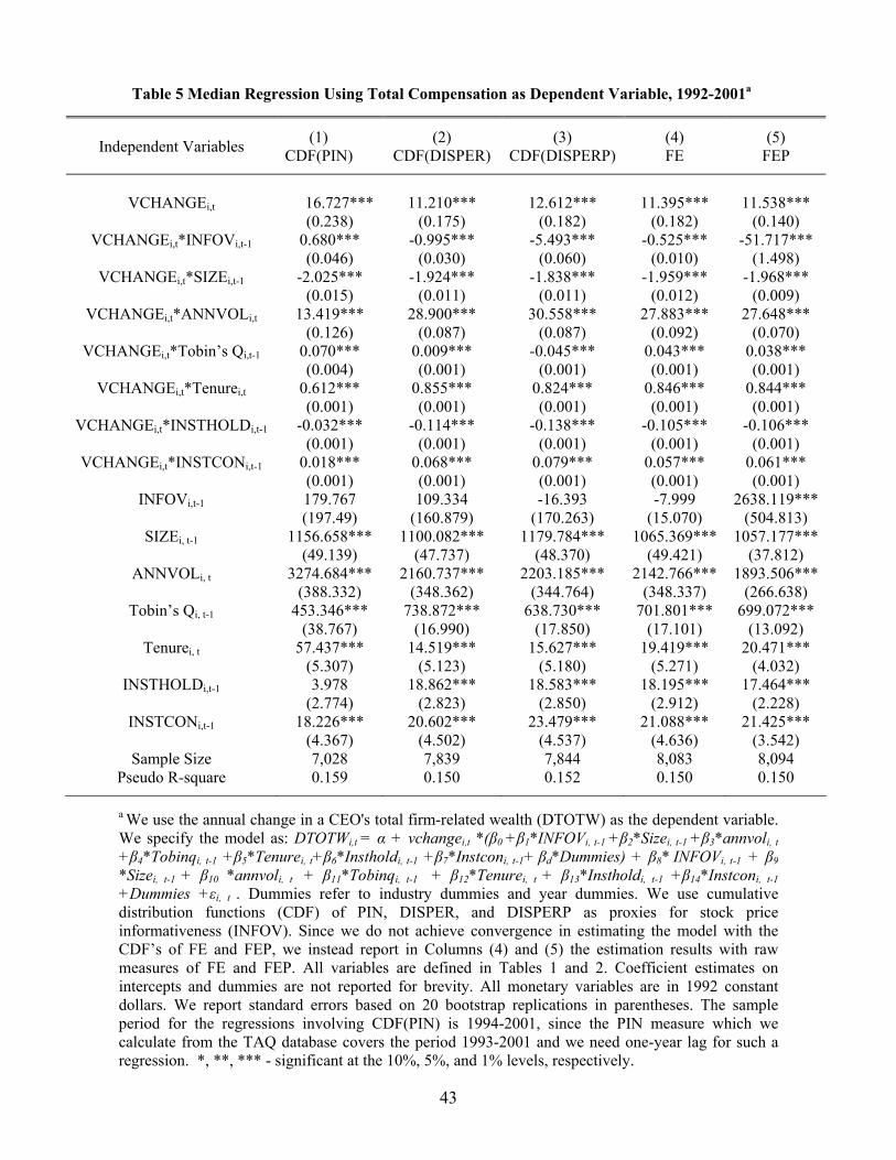
43

Table 5 Median Regression Using Total Compensation as Dependent Variable, 1992-2001a

Independent Variables

(1) CDF(PIN)

(2) CDF(DISPER)

(3) CDF(DISPERP)

(4) FE

(5) FEP

VCHANGEi,t

VCHANGEi,t*INFOVi,t-1

VCHANGEi,t*SIZEi,t-1

VCHANGEi,t*ANNVOLi,t

VCHANGEi,t*Tobin’s Qi,t-1

VCHANGEi,t*Tenurei,t

VCHANGEi,t*INSTHOLDi,t-1

VCHANGEi,t*INSTCONi,t-1

INFOVi,t-1

SIZEi, t-1

ANNVOLi, t

Tobin’s Qi, t-1

Tenurei, t

INSTHOLDi,t-1

INSTCONi,t-1

Sample Size

Pseudo R-square

16.727***

(0.238) 0.680*** (0.046)

-2.025*** (0.015)

13.419*** (0.126)

0.070*** (0.004)

0.612*** (0.001)

-0.032*** (0.001)

0.018*** (0.001) 179.767 (197.49)

1156.658*** (49.139)

3274.684*** (388.332)

453.346*** (38.767)

57.437*** (5.307) 3.978

(2.774) 18.226***

(4.367) 7,028 0.159

11.210***

(0.175) -0.995***

(0.030) -1.924***

(0.011) 28.900***

(0.087) 0.009*** (0.001)

0.855*** (0.001)

-0.114*** (0.001)

0.068*** (0.001) 109.334

(160.879) 1100.082***

(47.737) 2160.737***

(348.362) 738.872***

(16.990) 14.519***

(5.123) 18.862***

(2.823) 20.602***

(4.502) 7,839 0.150

12.612***

(0.182) -5.493***

(0.060) -1.838***

(0.011) 30.558***

(0.087) -0.045***

(0.001) 0.824*** (0.001)

-0.138*** (0.001)

0.079*** (0.001) -16.393

(170.263) 1179.784***

(48.370) 2203.185***

(344.764) 638.730***

(17.850) 15.627***

(5.180) 18.583***

(2.850) 23.479***

(4.537) 7,844 0.152

11.395***

(0.182) -0.525***

(0.010) -1.959***

(0.012) 27.883***

(0.092) 0.043*** (0.001)

0.846*** (0.001)

-0.105*** (0.001)

0.057*** (0.001) -7.999

(15.070) 1065.369***

(49.421) 2142.766***

(348.337) 701.801***

(17.101) 19.419***

(5.271) 18.195***

(2.912) 21.088***

(4.636) 8,083 0.150

11.538***

(0.140) -51.717***

(1.498) -1.968***

(0.009) 27.648***

(0.070) 0.038*** (0.001)

0.844*** (0.001)

-0.106*** (0.001)

0.061*** (0.001)

2638.119*** (504.813)

1057.177*** (37.812)

1893.506*** (266.638)

699.072*** (13.092)

20.471*** (4.032)

17.464*** (2.228)

21.425*** (3.542) 8,094 0.150

a We use the annual change in a CEO's total firm-related wealth (DTOTW) as the dependent variable. We specify the model as: DTOTWi,t = α + vchangei,t *(β0 +β1*INFOVi, t-1 +β2*Sizei, t-1 +β3*annvoli, t +β4*Tobinqi, t-1 +β5*Tenurei, t+β6*Instholdi, t-1 +β7*Instconi, t-1+ βd*Dummies) + β8* INFOVi, t-1 + β9 *Sizei, t-1 + β10 *annvoli, t + β11*Tobinqi, t-1 + β12*Tenurei, t + β13*Instholdi, t-1 +β14*Instconi, t-1 +Dummies +εi, t . Dummies refer to industry dummies and year dummies. We use cumulative distribution functions (CDF) of PIN, DISPER, and DISPERP as proxies for stock price informativeness (INFOV). Since we do not achieve convergence in estimating the model with the CDF’s of FE and FEP, we instead report in Columns (4) and (5) the estimation results with raw measures of FE and FEP. All variables are defined in Tables 1 and 2. Coefficient estimates on intercepts and dummies are not reported for brevity. All monetary variables are in 1992 constant dollars. We report standard errors based on 20 bootstrap replications in parentheses. The sample period for the regressions involving CDF(PIN) is 1994-2001, since the PIN measure which we calculate from the TAQ database covers the period 1993-2001 and we need one-year lag for such a regression. *, **, *** - significant at the 10%, 5%, and 1% levels, respectively.

44

Table 6 Median Regression of CEO Stock-Based Pay-Performance Sensitivity (PPS): Using Different Combinations of the CDFs of the Price Informativeness Measures, 1992-2001a

(1) (2) (3)

(4)

(5) (6)

Intercept

CDF(PINi, t-1)

CDF(FEi,t-1)

CDF(FEPi,t-1)

CDF(DISPERi,t-1)

CDF(DISPERPi,t-1)

SIZEi, t-1

ANNVOLi, t

Tobin’s Qi, t-1

Tenurei, t

INSTHOLDi,t-1

INSTCONi,t-1

Sample Size Pseudo R-square

11.331***

(2.132) 3.240*** (0.673)

-1.257** (0.537)

-1.910***

(0.165) 13.074***

(1.487) 1.126*** (0.132) 0.846** (0.016)

-0.102*** (0.010)

0.065*** (0.015)

3,905 0.104

11.096***

(2.363) 3.007*** (0.749)

-1.091* (0.651)

-1.853*** (0.182)

13.575*** (1.671)

1.194*** (0.147)

0.815*** (0.018)

-0.095*** (0.011)

0.057*** (0.016)

3,805 0.105

10.859***

(2.214) 3.041*** (0.694)

-2.962*** (0.584)

-1.884*** (0.171)

13.638*** (1.517)

0.980*** (0.138)

0.846*** (0.017)

-0.097*** (0.100)

0.079*** (0.015)

3,908 0.105

12.057***

(2.046) 2.593*** (0.643)

-4.355*** (0.597)

-1.815*** (0.156)

15.490*** (1.407)

0.725*** (0.130)

0.803*** (0.016)

-0.096*** (0.009)

0.073*** (0.014)

3,805 0.107

11.791***

(2.132) 2.444*** (0.669)

-0.972 (0.655)

-3.788*** (0.726)

-1.820*** (0.163)

15.302*** (1.466)

0.740*** (0.136)

0.804*** (0.016)

-0.093*** (0.100)

0.078*** (0.015)

3,791 0.107

12.832***

(1.890) 2.654*** (0.589) -0.322 (1.790) -0.335 (1.999)

-4.565*** (1.378)

-7.653*** (1.594)

-1.874*** (0.145)

14.765*** (1.312)

0.649*** (0.120)

0.808*** (0.014)

-0.104*** (0.008)

0.071*** (0.013)

3,788 0.108

aThe dependent variable is the CEO’s stock-based pay-performance sensitivity (PPS), which is defined as the change in value of the CEO’s stock and stock options holdings per $1,000 change in shareholder value. We specify the basic model as: PPSi,t = γ0 + γc*CINFOVi, t-1 + γ2* Sizei, t-1 + γ3* annvoli, t + γ4*Tobinqi, t-1 + γ5*Tenurei, t + γ6*INSTHOLDi, t-1 + γ7*INSTCONi, t-1+ industry dummies + year dummies+ εi, t , where CINFOV’s are various combinations of five price informativeness measures. We use the cumulative distribution functions (CDFs) of the five price informativeness measures in the regressions. We include CDF(PIN) in each combination. Coefficient estimates on industry dummies and year dummies are not reported for brevity. All monetary variables are in 1992 constant dollars. We report standard errors based on 20 bootstrap replications in parentheses. The sample period for regressions involving CDF(PIN) is 1994-2001, since the PIN measure which we calculate from the TAQ database covers the period 1993-2001 and we need one-year lag for such regressions. *, **, and *** - significant at the 10%, 5%, and 1% levels, respectively.

45

Table 7 Median Regression of CEO Total Pay-Performance Sensitivity (PPS_TOT): Using CDFs of the Stock Price Informativeness Measures, 1992-2001

Independent Variables

(1) (2) (3)

(4) (5)

Intercept

CDF(PINi, t-1)

CDF(FEi,t-1)

CDF(FEPi,t-1)

CDF(DISPERi,t-1)

CDF(DISPERPi,t-1)

SIZEi, t-1

ANNVOLi, t

Tobin’s Qi, t-1

Tenurei, t

INSTHOLDi,t-1

INSTCONi,t-1

Sample Size Pseudo R-square

14.517***

(2.050) 4.180*** (0.640)

-2.480*** (0.156)

18.212*** (1.287)

1.485*** (0.126)

0.984*** (0.017)

-0.092*** (0.009)

0.054*** (0.014)

6,724 0.103

18.676***

(2.772)

-3.632*** (0.725)

-2.907***

(0.208) 9.744*** (1.555)

1.833*** (0.074)

1.428*** (0.023)

-0.188*** (0.013)

0.168*** (0.020)

7,053 0.121

20.215***

(2.529)

-7.715*** (0.676)

-2.931***

(0.189) 11.108***

(1.381) 1.368*** (0.069)

1.435*** (0.021)

-0.184*** (0.011)

0.186*** (0.018)

7,061 0.123

18.576***

(2.886)

-4.740***

(0.767)

-2.765***

(0.216) 12.366***

(1.635) 1.670*** (0.077)

1.377*** (0.024)

-0.181*** (0.013)

0.157*** (0.021)

6,851 0.121

22.646***

(3.084)

-11.143*** (0.850)

-2.863*** (0.230)

11.919*** (1.695)

0.978*** (0.085)

1.393*** (0.026)

-0.189*** (0.014)

0.186*** (0.022)

6,856 0.124

a The dependent variable is the CEO’s total pay-performance sensitivity (PPS_TOT), which measures the dollar value change in CEO’s total direct compensation and stock-based compensation per $1,000 increase in shareholder value. We specify the model as: PPS_TOTi,t = γ0 + γ1*INFOVi, t-1 + γ2* Sizei, t-1 + γ3* annvoli, t + γ4*Tobinqi, t-1 + γ5*Tenurei, t + γ6*INSTHOLDi, t-1 + γ7*INSTCONi, t-1+ industry dummies + year dummies+ εi, t . We use the cumulative distribution functions (CDFs) of five price informativeness variables in the regressions. Coefficient estimates on industry dummies and year dummies are not reported for brevity. All monetary variables are in 1992 constant dollars. We report standard errors based on 20 bootstrap replications in parentheses. The sample period for the regression involving CDF(PIN) is 1994-2001, since the PIN measure which we calculate from the TAQ database covers the period 1993-2001 and we need one-year lag for such a regression. *, **, and *** - significant at the 10%, 5%, and 1% levels, respectively.

46

Table 8 Median Regression of the CEO Pay-Performance Sensitivity: Subperiod Analysisa Panel A: 1992-1999 Panel B: 2000-2001

(1) CDF

(PINi,t-1)

(2) CDF

(FEi, t-1)

(3) CDF

(FEPi, t-1)

(4) CDF(DISP

ERi, t-1)

(5) CDF(DISP

ERPi, t-1)

(1)’ CDF

(PINi,t-1)

(2)’ CDF

(FEi, t-1)

(3)’ CDF

(FEPi, t-1)

(4)’ CDF(DISP

ERi, t-1)

(5)’ CDF(DISP

ERPi, t-1)

Intercept

CDF(INFOVi, t-1 )

SIZEi, t-1

ANNVOLi, t

Tobin’s Qi, t-1

Tenurei,t

INSTHOLDi,t-1

INSTCONi,t-1

Sample Size Pseudo R-square

12.523*** (2.403)

2.442*** (0.714)

-2.292*** (0.185)

21.314*** (1.631)

1.501*** (0.155)

0.928*** (0.019)

-0.089*** (0.010)

0.053*** (0.016)

4,963 0.097

14.116*** (3.247)

-2.603*** (0.810)

-2.861*** (0.250)

10.293*** (1.982)

3.682*** (0.125)

1.324*** (0.025)

-0.199*** (0.014)

0.181*** (0.023)

5,303 0.127

15.670*** (2.995)

-5.757*** (0.770)

-2.916*** (0.230)

11.051*** (1.788)

3.293*** (0.118)

1.328*** (0.023)

-0.201*** (0.013)

0.195*** (0.021)

5,310 0.128

13.679*** (3.897)

-2.732*** (1.002)

-2.692*** (0.300)

11.585*** (2.416)

3.647*** (0.152)

1.265*** (0.031)

-0.191*** (0.017)

0.164*** (0.028)

5,132 0.127

18.061*** (3.431)

-7.549*** (0.915)

-2.918*** (0.263)

12.952*** (2.076)

3.048*** (0.139)

1.264*** (0.027)

-0.197*** (0.015)

0.167*** (0.024)

5,137 0.129

14.849*** (3.791)

9.443*** (1.336)

-2.201*** (0.284)

15.009*** (2.088)

1.141*** (0.209)

1.248*** (0.037)

-0.059*** (0.018) -0.005 (0.030)

1,761 0.117

25.019*** (4.622)

-2.619** (1.331)

-2.628*** (0.321)

10.932*** (2.208)

0.544*** (0.083)

1.426*** (0.044)

-0.129*** (0.022) 0.036

(0.037)

1,750 0.122

26.413*** (5.324)

-4.711*** (1.572)

-2.770*** (0.368)

9.881*** (2.453)

0.474*** (0.100)

1.430*** (0.050)

-0.127*** (0.025) 0.055

(0.043)

1,751 0.123

23.305*** (4.266)

-4.544*** (1.221)

-2.435*** (0.295)

12.129*** (2.039)

0.476*** (0.076)

1.444*** (0.040)

-0.147*** (0.02) 0.054

(0.035)

1,719 0.124

24.705*** (4.628)

-9.754*** (1.429)

-2.532*** (0.317)

12.566*** (2.135) 0.178** (0.083)

1.444*** (0.044)

-0.137*** (0.021) 0.088** (0.037)

1,719 0.127

a We divide the sample into two subperiods: 1992-1999 and 2000-2001. For each subperiod, we specify the model as: PPSi,t = γ0 + γ1*INFOVi, t-1 + γ2* Sizei, t-1 + γ3* annvoli, t + γ4*Tobinqi, t-1 + γ5*Tenurei, t + γ6*INSTHOLDi, t-1 + γ7*INSTCONi, t-1+ industry dummies + year dummies+ εi, t . We use the CDFs of the five price informativeness measures in the regressions and report their respective parameter estimates in the second row. Coefficient estimates on industry dummies and year dummies are not reported for brevity. All monetary variables are in 1992 constant dollars. We report standard errors based on 20 bootstrap replications in parentheses. The sample period for the regressions involving CDF(PIN) is 1994-2001, since the PIN measure which we calculate from the TAQ database covers the period 1993-2001 and we need one-year lag for such regressions. *, **, *** - significant at the 10%, 5%, and 1% levels, respectively.

47

Table 9 Robustness Analysis on Filtered Samples a

INFOVi,t-1 Sample

Size Pseudo

R-square

Panel A Filtering by the autocorrelations of the daily trading volumes (AR) (1) deleting firms with AR above the 70% level (CDF(PIN)) (2) deleting firms with AR above the 90% level (CDF(PIN) ) Panel B Filtering by the KZ Index (3) deleting firms with the KZ index above the 70% (CDF(PIN)) (4) deleting firms with the KZ index above the 70% level (CDF(FEP)) (5) deleting firms with the KZ index above the 90% (CDF(PIN)) (6) deleting firms with the KZ index above the 90% level (CDF(FEP)) Panel C Filtering by the MAD (7) deleting firms engaging in M&As (CDF(PIN)) (8) deleting firms engaging in M&As (CDF(FEP)) Panel D Filtering by multiple variables (9) deleting firms with the KZ index above the 70% level or MAD =1 (CDF(PIN)) (10) deleting firms with the KZ index above the 70% level or MAD =1 (CDF(FEP))

4.633*** (0.698)

3.852*** (0.669)

4.162*** (0.820)

-5.147*** (1.119)

3.704*** (0.638)

-6.961*** (0.898)

4.357*** (0.716)

-6.596*** (0.747)

4.638*** (0.865)

-4.843*** (1.127)

4,939

6,205

4,795

4,892

6,142

6,460

6,015

6,305

4,341

4,461

0.101

0.100

0.107

0.131

0.104

0.126

0.100

0.123

0.104

0.132

aThe dependent variable is the CEO’s stock-based pay-performance sensitivity (PPS). We specify the model as: PPSi,t = γ0 + γ1*INFOVi, t-1 + γ2* Sizei, t-1 + γ3* annvoli, t + γ4*Tobinqi, t-1 + γ5*Tenurei, t + γ6*INSTHOLDi, t-1 + γ7*INSTCONi, t-1+ industry dummies + year dummies+ εi, t . For brevity, we only report the estimated coefficients of the various information variables. We first calculate the autocorrelation of daily trading volumes (AR) for each firm on an annual basis. Models 1 and 2 reports the results of deleting firms, whose ARs are above 70% and 90% levels respectively. We then compute the KZ index based on the specification given in Kaplan and Zingales (1997). Models 3-6 report the results of deleting firms whose KZ index levels are above the 70% or 90% levels. We define a dummy variable MAD, whose value is 1 if a firm engages in an M&A activity in a given year, and zero otherwise. We filter our sample in Models 7 and 8 based on MAD. In Models 9-10, we filter our samples based on multiple variables, as indicated in the table. The information variables used in each regression is also indicated in the table. *, **, and *** - significant at the 10%, 5%, and 1% levels, respectively.

48

Table 10 Median Regression of the Pay-Performance Sensitivity: All Executives a Panel A: Dependent variable = PPS_EXE Panel B: Dependent Variable = PPS_TEAM

(1) CDF

(PINI,t-1)

(2) CDF

(FEi, t-1)

(3) CDF

(FEPi, t-1)

(4) CDF(DISP

ERi, t-1)

(5) CDF(DISP

ERPi, t-1)

(1)’ CDF

(PINI,t-1)

(2)’ CDF

(FEi, t-1)

(3)’ CDF

(FEPi, t-1)

(4)’ CDF(DISP

ERi, t-1)

(5)’ CDF(DISP

ERPi, t-1)

Intercept

CDF(INFOVi, t-1 )

SIZEi, t-1

ANNVOLi, t

Tobin’s Qi, t-1

Tenurei,t

CEOFALG

INSTHOLDi,t-1

INSTCONi,t-1

Sample Size

Pseudo R-square

5.437*** (0.219)

0.820*** (0.068)

-0.603*** (0.017)

3.062*** (0.138)

0.184*** (0.013)

__

6.042*** (0.033) -0.001 (0.001)

-0.011*** (0.002)

28,736 0.061

5.507*** (0.260)

-0.698*** (0.068)

-0.660*** (0.020)

4.143*** (0.148)

0.255*** (0.007)

__

8.814*** (0.041)

-0.009*** (0.001) 0.005** (0.002) 29,787 0.071

6.093*** (0.243)

-1.332*** (0.065)

-0.709*** (0.018)

4.152*** (0.135)

0.216*** (0.007)

__

8.828*** (0.038)

-0.007*** (0.001)

0.005*** (0.002) 29,817 0.071

5.594*** (0.258)

-1.056*** (0.069)

-0.650*** (0.019)

4.539*** (0.149)

0.227*** (0.007)

__

8.451*** (0.041)

-0.007*** (0.001) 0.004* (0.002) 28,962 0.071

6.415*** (0.278)

-2.006*** (0.077)

-0.707*** (0.021)

4.297*** (0.155)

0.164*** (0.008)

__

8.396*** (0.043)

-0.007*** (0.001)

0.007*** (0.002) 28,982 0.072

34.633*** (4.207)

9.832*** (1.280)

-5.153*** (0.318)

31.472*** (2.614)

3.815*** (0.258)

1.315*** (0.034)

__

-0.191*** (0.018) 0.062** (0.029) 5,378 0.126

49.505*** (5.502)

-5.157*** (1.426)

-6.162*** (0.411)

15.237*** (3.005)

2.879*** (0.138)

1.837*** (0.044)

__

-0.345*** (0.025)

0.264*** (0.040) 5,839 0.145

57.527*** (6.219)

-14.471*** (1.646)

-6.535*** (0.465)

16.049*** (3.306)

2.380*** (0.159)

1.819*** (0.049)

__

-0.369*** (0.028)

0.283*** (0.045) 5,847 0.147

51.907*** (6.172)

-9.727*** (1.617)

-6.121*** (0.461)

19.155*** (3.400)

2.763*** (0.154)

1.745*** (0.050)

__

-0.337*** (0.028)

0.247*** (0.045) 5,664 0.145

57.072*** (5.068)

-22.431*** (1.365)

-6.134*** (0.377)

21.843*** (2.709)

1.647*** (0.128)

1.738*** (0.040)

__

-0.365*** (0.023)

0.307*** (0.036) 5,667 0.151

a In Panel A, the dependent variable is PPS_EXE, i.e., the pay-performance sensitivity of a top five high-paid executive, CEO included, of a firm. Since the tenure information is not available for non-CEO executives, we drop the variable Tenure from all regressions. CEOFLAG is a dummy variable equal to 1 for CEOs and 0 otherwise. In Panel B, the dependent variable is PPS_TEAM. We sum up PPS_EXE’s across all top five high-paid executives of a firm in a fiscal year to obtain PPS_TEAM. Tenure refers to CEO tenure and CEOFLAG is excluded from all regressions. In both Panels A and B we use the CDFs of the five price informativeness measures. Coefficient estimates on industry dummies and year dummies are not reported for brevity. All monetary variables are in 1992 constant dollars. We report standard errors based on 20 bootstrap replications in parentheses. The sample period for the regressions involving CDF(PIN) is 1994-2001. *, **, *** - significant at the 10%, 5%, and 1% levels, respectively.