Stock Market, Economic Performance, And Presidential ... · Roger W. Mayer, Walden University, USA...

Title Stock Market, Economic Performance, And PresidentialElections

Author(s) Chien, WW; Mayer, R; Wang, Z

Citation Journal of Business & Economics Research, , v. 12 n. 2, p. 159-170

Issued Date

URL http://hdl.handle.net/10722/222295

Rights This work is licensed under a Creative Commons Attribution-NonCommercial-NoDerivatives 4.0 International License.

Journal of Business & Economics Research – Second Quarter 2014 Volume 12, Number 2

Copyright by author(s); CC-BY 159 The Clute Institute

Stock Market, Economic Performance,

And Presidential Elections Wen-Wen Chien, State University of New York at Old Westbury, USA

Roger W. Mayer, Walden University, USA

Zigan Wang, Columbia University, USA

ABSTRACT

Using stock market and economic data from 1900 to 2008 from 27 separate presidential

administrations in the United States (U.S.), including 15 Republican and 12 Democratic, this paper

examines the relationships between the market return after each Election Day and economic

performance during the presidential term. Using the theoretical framework of political economy,

the authors examine how Wall Street’s reaction to a presidential election acts as a predictive

measure of future economic performance. The analysis shows that the after-election market

movement has progressively been more accurate in predicting the future Gross Domestic Product

(GDP) growth but not the future unemployment rates. Given that the results show a higher

correlation over time, the model appears to provide a good starting point for judging the economic

potential of future presidential administrations.

Keywords: Market Return; Economic Performance; GDP Growth; Unemployment

INTRODUCTION

.S. presidential elections and the stock market are popular topics for research (Wisniewski, Lightfoot, &

Lilley, 2012). The reason for this interest is because policies established by the governing president affect

the ability of businesses and the general economy to prosper. The political economy theoretical

framework provides a basis for understanding the relationship between politics and the economy. Gilpin (2001)

describes this relationship as “interactive.” As is seen from the prism of historic events, business attempts to promote

a political agenda that supports their goals (Caro, 2002). The reason that some business sectors are willing to spare

massive amounts of money to promote a specific candidate or political agenda is because the winning candidate’s

agenda has a direct impact on the business environment. Allvine and O’Neil (1980) documented the interaction

between politics and the market by demonstrating that markets generally follow a four-year business cycle that

corresponds to the presidential election cycle. The authors’ research adds to this perspective by increasing their

understanding of how well business and investors gauge the final decision of a presidential election.

Prior researchers examined various elements of the election process to understand the relationship between

the presidential performance variables and stock market performance. These studies are generally predictive in nature.

Niederhoffer, Gibbs, and Bullock (1970) documented the changes of Dow Jones Industrial Average (DJI) before and

after election and nominating conventions for 18 presidents from 1900 to 1968. They also document the one-day,

one-week and one-month DJI changes after the events and DJI changes during each of the four years under each

president's administration, reaching a conclusion that the stock market performances during Republican and

Democratic administrations have no systematic difference. Using data between 1927 and 1998, Santa-Clara and

Valkanov (2003) determined that the stock market’s excess return is higher under Democratic than Republican

presidencies and the difference is from higher real stock returns and lower real interest rates but is not explained by

business-cycle variables and is not concentrated around election dates.

Goodell and Vähämaa (2013) demonstrated that the presidential election process creates market uncertainty

as investors develop expectations regarding potential winners and future macroeconomic policy. Goodell and Bodey

(2012) determined that as the probable winner of the election becomes clearer, volatility decreases and markets react

U



negatively with decreases in P/E ratios. Riley and Luksetich (1980) suggest that the results are dependent upon what

party becomes the clear winner. Huang (1985) documents the higher average returns during Democratic

administrations, in contrast of the widely held belief that the Republican Party is better at business. Moreover, findings

from Johnson, Chittenden, and Jensen (1999) also indicate that the returns to small-cap stocks are substantially higher

during Democratic administrations.

The analysis shows that the after-election market movement has progressively been more accurate in

predicting the future GDP growth but not the future unemployment rates. Given that the researchers see a higher

correlation over time, their model appears to provide a good starting point for judging the economic potential of new

presidential administrations. An additional finding that was not part of the hypothesis was that Republicans tend to

govern in an economy with unemployment rates that increase during the course of their term. Democrats tend to

preside over an economy with higher unemployment rates at the beginning of their terms and that tend to decrease over

time.

The reminder of this paper consists of the research question and hypotheses, research model and data used to

test hypotheses, empirical results, and a conclusion.

RESEARCH QUESTION AND HYPOTHSES

The overreaching research question for this study is, “to what extent does the stock price change immediately

after a presidential election relate to or predict the presidential administration’ economic performance as defined by

GDP growth and unemployment?”

H1: There is a relationship between the GDP growth during the term of a presidential administration and the

change in stock price immediately after the presidential election.

H2: There is a relationship between unemployment rates during the term of a presidential administration and the

change in stock price immediately after the presidential election.

Instead of confining their research to just market reactions to the new president, the researchers examined the

relationship between the market's perspective of each president and the economic performance under each one,

including GDP growth and the unemployment rate. The goal of this research is to determine if the market is able to

predict the impact of a president on the economy. The hypotheses are based on the assumption that the stock market

movement reflects people's perspective of the future economy. The generalized assumption is in the statement that

when people are positive about the future, the stock market reflects this attitude and increases. Conversely, when

people have a pessimistic view of the future the market reflects this attitude and decreases. The efficient market

hypothesis suggests that the market responds to the election winners with all the available information about the

winning candidate. Thus, the prediction of an efficient market should be right (Fama, 1970). If the market moves up

after the election, it suggests that the market generally approves the winner's capability of making the economy grow;

if the market drops, it suggests that the investors are pessimistic about the economy in the future. To the authors’

knowledge, there has not been any research verifying the accuracy of the market's prediction and this paper will fill in

this gap.

RESEARCH MODEL

To test the hypothesis, the researchers use the simple OLS linear regression model to address the correlation

between the 1-day DJI change following the Election Day and the economic indicators, the four-year cumulative GDP

growth rate and average unemployment rate. The formula of the model is:

0 1 2t t t tEI DJI X

where EI is the specific economic indicator. The researchers used two separate indicators, including the four-year

cumulative GDP growth rate in regressions (1) – (4) and the average unemployment rate in regressions (5) – (6). DJI is

the 1-day DJI percentage change following the Election Day. X is the other explanatory variable, or the four-year lag



cumulative GDP growth rate in regressions (1) and (3). The lag GDP growth is a common independent variable for

explaining or predicting the GDP growth rate.

DATA

The DJI was used to measure the market movement around the Election Day because it has a longer range

than any other market indices and it traces back to before 1900. The data include stock market and economic

information from 1900 to 2008 across 27 administrations with 15 of them Republican and 12 Democratic. Table 1

summarizes the DJI closing price of selected dates in each election year’s November and December around the

Election Day since 1900. All data is publicly available; DJI was extracted from Bloomberg.1 Some data reported by

Bloomberg were different compared to the dataset used by Niederhoffer et al. (1970). The researchers were unable to

determine the source of this error; however, the differences did not affect the results of hypothesis testing. In 1984, the

NYSE opened on Election Day for the first time in its 192-year history. So, starting in 1984, the data used was the

Election Day (Tuesday) closing price rather than the price on Monday before Election Day.

Table 1 (as well as Table 3) shows that among the 13 times that the Democratic Party won the elections, the

DJI dropped nine times after the Election Day and among the 15 times when the Republicans won, the market rose ten

times during Wednesday. The sample does not include Obama’s victory in 2012, but the DJI dropped on Wednesday

after the election. Therefore, since 1900, the market has responded negatively to the Democratic Party’s winning for

10 out of 14 times in total.

A correlation analysis concludes that the DJI change on Wednesday is closely correlated to the DJI

movement within the election week (Friday). In addition, it correlates with the DJI movement within two weeks (the

next Friday) and the DJI return within a month after the election. For brevity, the researchers did not include this

analysis in the tables.

Table 2 summarizes the yearly GDP growth and unemployment rates since 1900. GDP growth data from

1901 to 1996 are from Angus Maddison's (2008) Historical Statistics of the World Economy: 1-2008 AD. GDP growth

data from 1997 to 2011 are from the World Bank. GDP growth in 2012 is from the U.S. Bureau of Economic Analysis.

The researchers obtained unemployment rates from various sources. Unemployment rates from 1901 to 1930 are from

Romer (1986), data from 1931 to 1940 are from Darby (1976), data from 1941 to 1947 are from Barro (1977), and data

after 1948 are from the U.S. Bureau of Labor Statistics. The data used for this study comes from the “age 16 and over”

category (U.S. Bureau of Labor Statistics, 2013). According to Barro (1977), the annual average unemployment rates

(data are given in the Economic Report of the President) are based on the total labor force, which includes military

personnel. Data for 1941-43 is adjusted for treatment of government “emergency workers,” as discussed by Darby

(1976). Cumulative GDP growth and average unemployment rate are calculated according to each year’s data.

There were some winning candidates who did not finish their four-year presidency for various reasons. In

recent times, this includes John F. Kennedy who was assassinated and Richard Nixon who resigned in his second term.

In each case, the Vice-President took over and completed the terms. Therefore, the economic performance of those

years should be attributed to combined administration rather than to any single president.

1 http://www.bloomberg.com/markets/stocks/



Table 1: Summary of Dow Jones Industrial Average (DJI) Around Election Day*

Yea

r

Ele

ctio

n W

inn

er

Pa

rty

DJ

I B

efo

re E

lect

ion

*

Ele

ctio

n D

ay

DJ

I W

edn

esd

ay

DJ

I 1

-Day

Ch

an

ge

(%)

DJ

I F

rid

ay

DJ

I 3

-Day

Ch

an

ge

(%)

DJ

I N

ext

Fri

da

y

DJ

I 1

-Wee

k C

han

ge

(%)

DJ

I N

ext

Mo

nth

(in

21

Tra

din

g D

ay

s)

DJ

I 1

-Mo

nth

Ch

an

ge

(%)

DJ

I in

4

Yea

rs (

in 1

000

Tra

din

g D

ay

s)

DJ

I 4

-Yea

r C

ha

ng

e

(%)

190

0 William McKinley (R) 60.87 11/6/190

0 62.9 3.33 65.15 7.03 68.19 12.03 65.07 6.90 63.72 4.68

190

4 Theodore Roosevelt (R) 66.21 11/8/190

4 67.07 1.30 68.03 2.75 69.69 5.26 68 2.70 82.22 24.18

190

8 William Howard Taft (R) 82.9 11/3/190

8 84.87 2.38 87.28 5.28 88.38 6.61 86.58 4.44 91.44 10.30

191

2 Woodrow Wilson (D) 90.29 11/5/191

2 91.94 1.83 91.31 1.13 90.09 -0.22 87.88 -2.67 95.05 5.27

191

6 Woodrow Wilson (D) 107.21 11/7/191

6 106.83 -0.35 107.7 0.41 109.62 2.25 106.43 -0.73 76.65 -28.5

0 192

0 Warren G. Harding (R) 85.48 11/2/192

0 84.99 -0.57 83.48 -2.34 77.56 -9.27 77.3 -9.57 101.96 19.28

192

4 Calvin Coolidge (R) 103.89 11/4/192

4 105.11 1.17 104.9 0.93 108.96 4.88 111.56 7.38 257.13 147.5

0 192

8 Herbert Hoover (R) 257.58 11/6/192

8 260.68 1.20 263.1 2.12 276.66 7.41 279.79 8.62 61.86 -75.9

8 193

2 Franklin D. Roosevelt (D) 64.58 11/8/193

2 61.67 -4.51 68.03 5.34 62.96 -2.51 60.05 -7.01 182.25 182.2

1 193


6 180.66 2.26 181.6 2.79 182.65 3.38 180.97 2.43 132.45 -25.0

3 194


0 131.98 -2.39 136.6 1.06 134.74 -0.35 130.33 -3.61 148.87 10.10

194


4 147.52 -0.27 148.1 0.11 145.77 -1.45 149.23 0.89 188.28 27.29

194

8 Harry S Truman (D) 189.76 11/2/194

8 182.46 -3.85 178.4 -6.00 176.01 -7.25 175 -7.78 265.83 40.09

195

2 Dwight D. Eisenhower (R) 270.22 11/4/195

2 271.29 0.40 273.5 1.20 274.44 1.56 282.05 4.38 490.18 81.40

195

6 Dwight D. Eisenhower (R) 495.36 11/6/195

6 491.14 -0.85 485.3 -2.02 480.66 -2.97 492.73 -0.53 587.30 18.56

196

0 John F. Kennedy (D) 597.62 11/8/196

0 602.25 0.77 608.6 1.84 603.61 1.00 605.16 1.26 876.20 46.61

196

4 Lyndon Johnson (D) 875.5 11/3/196

4 873.81 -0.19 876.9 0.16 874.1 -0.16 870.78 -0.54 950.65 8.58

196

8 Richard Nixon (R) 946.23 11/5/196

8 949.47 0.34 959 1.35 963.7 1.85 977.69 3.32 930.46 -1.67

197

2 Richard Nixon (R) 984.8 11/7/197

2 983.74 -0.11 995.3 1.06 1005.57 2.11 1033.26 4.92 937.00 -4.85

197

6 Jimmy Carter (D) 966.09 11/2/197

6 956.53 -0.99 943.1 -2.38 927.69 -3.97 946.64 -2.01 959.90 -0.64

198

0 Ronald Reagan (R) 937.2 11/4/198

0 953.16 1.70 932.4 -0.51 986.35 5.24 970.48 3.55 1195.89 27.60

198

4 Ronald Reagan (R) 1229.24 11/6/198

4 1233.22 0.32 1219 -0.84 1187.94 -3.36 1170.49 -4.78 2183.50 77.63

198

8 George Bush (R) 2124.64 11/8/198

8 2118.24 -0.30 2067 -2.71 2062.41 -2.93 2141.71 0.80 3200.88 50.66

199

2 Bill Clinton (D) 3262.21 11/3/199

2 3223.04 -1.20 3240 -0.68 3233.03 -0.89 3276.53 0.44 6059.19 85.74

199

6 Bill Clinton (D) 6041.67 11/5/199

6 6177.71 2.25 6220 2.95 6348.03 5.07 6437.1 6.55 10271.72 70.01

200

0 George W. Bush (R) 10977.21 11/7/200

0 10907.06 -0.64 10603 -3.41 10629.9 -3.16 10617.36 -3.28 10137.05 -7.65

200

4 George W. Bush (R) 10054.39 11/2/200

4 10137.05 0.82 10388 3.31 10539 4.82 10585.12 5.28 8519.21 -15.2

7 200

8 Barack Obama (D) 9625.28 11/4/200

8 9139.27 -5.05 8944 -7.08 8497.31 -11.72 8635.42 -10.28 13077.34 35.86

* DJI closing price of the day just before election results were revealed, which was Monday before 1980 and Tuesday since 1984.



Table 2: Summary of Yearly GDP Growth and Unemployment Rate under Each President's Administration

President

Pa

rty

First Year Second Year Third Year Fourth Year All Four Years

Yea

r

GD

P G

row

th

Un

emp

loym

ent

Ra

te

Yea

r

GD

P G

row

th

Un

emp

loym

ent

Ra

te

Yea

r

GD

P G

row

th

Un

emp

loym

ent

Ra

te

Yea

r

GD

P G

row

th

Un

emp

loym

ent

Ra

te

Cu

mu

lati

ve

GD

P G

row

th

Av

erag

e

Un

emp

loym

ent

Ra

te

W. McKinley/T. Roosevelt (R) 1901 11.3 4.59 1902 1.04 4.30 1903 4.86 4.35 1904 -1.26 5.08 16.395 4.580

Theodore Roosevelt (R) 1905 7.40 4.62 1906 11.5 3.29 1907 1.54 3.57 1908 -8.19 6.17 11.657 4.413

William Howard Taft (R) 1909 12.2 5.13 1910 1.02 5.86 1911 3.26 6.27 1912 4.68 5.25 22.550 5.628

Woodrow Wilson (D) 1913 3.95 4.93 1914 -7.7 6.63 1915 2.82 7.18 1916 13.80 5.63 12.265 6.093

Woodrow Wilson (D) 1917 -2.50 5.23 1918 9.02 3.38 1919 0.87 2.95 1920 -0.95 5.16 6.201 4.180

W. G. Harding/C. Coolidge (R) 1921 -2.27 8.73 1922 5.53 6.93 1923 13.2 4.80 1924 3.06 5.80 20.310 6.565

Calvin Coolidge (R) 1925 2.32 4.92 1926 6.52 4.02 1927 1.0 4.57 1928 1.12 5.02 11.314 4.633

Herbert Hoover (R) 1929 6.12 4.61 1930 -8.9 8.94 1931 -7.8 15.3 1932 -13.20 22.90 -22.530 12.938

Franklin D. Roosevelt (D) 1933 -2.10 20.60 1934 7.73 16.00 1935 7.65 14.20 1936 14.21 9.90 29.669 15.175

Franklin D. Roosevelt (D) 1937 4.28 9.10 1938 -3.98 12.50 1939 7.96 11.30 1940 7.73 9.50 16.456 10.600

Franklin D. Roosevelt (D) 1941 18.20 5.80 1942 20.01 2.90 1943 19.89 1.50 1944 8.38 1.00 84.318 2.800

F. D. Roosevelt/ H. Truman (D) 1945 -4.02 1.60 1946 -20.64 3.70 1947 -1.51 3.80 1948 3.78 3.80 -22.145 3.225

Harry S. Truman (D) 1949 0.39 5.90 1950 8.69 5.30 1951 7.61 3.30 1952 3.73 3.00 21.797 4.375

Dwight D. Eisenhower (R) 1953 4.60 2.90 1954 -0.66 5.50 1955 7.07 4.40 1956 1.95 4.10 13.426 4.225

Dwight D. Eisenhower (R) 1957 1.88 4.30 1958 -1.01 6.80 1959 7.42 5.50 1960 2.49 5.50 11.032 5.525

J. F. Kennedy/L. Johnson (D) 1961 2.33 6.70 1962 6.03 5.50 1963 4.32 5.70 1964 5.79 5.20 19.741 5.775

Lyndon Johnson (D) 1965 6.38 4.50 1966 6.55 3.80 1967 2.50 3.80 1968 4.76 3.60 21.712 3.925

Richard Nixon (R) 1969 3.13 3.50 1970 0.17 4.90 1971 3.12 5.90 1972 5.30 5.60 12.174 4.975

R. Nixon/G. R. Ford (R) 1973 5.68 4.90 1974 -0.28 5.60 1975 -0.28 8.50 1976 5.24 7.70 10.596 6.675

Jimmy Carter (D) 1977 4.53 7.10 1978 5.71 6.10 1979 3.40 5.80 1980 0.05 7.10 14.313 6.525

Ronald Reagan (R) 1981 2.50 7.60 1982 -1.87 9.70 1983 4.19 9.60 1984 7.28 7.50 12.427 8.600

Ronald Reagan (R) 1985 3.88 7.20 1986 3.44 7.00 1987 3.52 6.20 1988 4.21 5.50 15.919 6.475

George Bush (R) 1989 3.46 5.30 1990 1.75 5.60 1991 -0.19 6.80 1992 3.34 7.50 8.580 6.300

Bill Clinton (D) 1993 2.69 6.90 1994 4.06 6.10 1995 2.54 5.60 1996 3.75 5.40 13.682 6.000

Bill Clinton (D) 1997 4.50 4.90 1998 4.40 4.50 1999 4.90 4.20 2000 4.20 4.00 19.250 4.400

George W. Bush (R) 2001 1.10 4.70 2002 1.80 5.80 2003 2.60 6.00 2004 3.50 5.50 9.292 5.500

George W. Bush (R) 2005 3.10 5.10 2006 2.70 4.60 2007 1.90 4.60 2008 -0.40 5.80 7.464 5.025

Barack Obama (D) 2009 -3.50 9.30 2010 3.00 9.60 2011 1.70 9.00 2012 2.20 8.10 3.309 9.000

Average

3.63 6.10

2.34 6.24

3.93 6.24

3.23 6.30 14.33 6.22

Average since 1953

3.08 5.66

2.39 6.07

3.25 6.11

3.58 5.87 12.86 5.93

Average (Republican)

4.43 5.21

1.52 5.92

3.03 6.42

1.27 6.99 10.71 6.14

Average since 1953 (R)

3.26 5.06

0.67 6.17

3.26 6.39

3.66 6.08 11.21 5.92

Average (Democratic)

2.70 7.12

3.30 6.62

4.97 6.03

5.49 5.49 18.51 6.31

Average since 1953 (D) 2.82 6.57 4.96 5.93 3.23 5.68 3.46 5.57 15.33 5.94



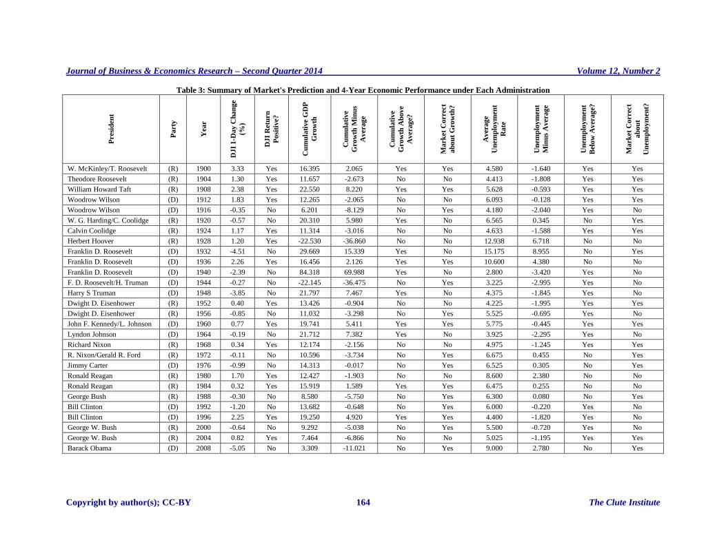
Table 3: Summary of Market's Prediction and 4-Year Economic Performance under Each Administration

Presi

den

t

Pa

rty

Yea

r

DJ

I 1

-Day

Ch

an

ge

(%)

DJ

I R

etu

rn

Po

siti

ve?

Cu

mu

lati

ve G

DP

Gro

wth

Cu

mu

lati

ve

Gro

wth

Min

us

Av

era

ge

Cu

mu

lati

ve

Gro

wth

Ab

ove

Av

era

ge?

Ma

rk

et

Correc

t

ab

ou

t G

row

th?

Av

era

ge

Un

em

plo

ym

en

t

Ra

te

Un

em

plo

ym

en

t

Min

us

Avera

ge

Un

em

plo

ym

en

t

Belo

w A

ver

ag

e?

Ma

rk

et

Correc

t

ab

ou

t

Un

em

plo

ym

en

t?

W. McKinley/T. Roosevelt (R) 1900 3.33 Yes 16.395 2.065 Yes Yes 4.580 -1.640 Yes Yes

Theodore Roosevelt (R) 1904 1.30 Yes 11.657 -2.673 No No 4.413 -1.808 Yes Yes

William Howard Taft (R) 1908 2.38 Yes 22.550 8.220 Yes Yes 5.628 -0.593 Yes Yes

Woodrow Wilson (D) 1912 1.83 Yes 12.265 -2.065 No No 6.093 -0.128 Yes Yes

Woodrow Wilson (D) 1916 -0.35 No 6.201 -8.129 No Yes 4.180 -2.040 Yes No

W. G. Harding/C. Coolidge (R) 1920 -0.57 No 20.310 5.980 Yes No 6.565 0.345 No Yes

Calvin Coolidge (R) 1924 1.17 Yes 11.314 -3.016 No No 4.633 -1.588 Yes Yes

Herbert Hoover (R) 1928 1.20 Yes -22.530 -36.860 No No 12.938 6.718 No No

Franklin D. Roosevelt (D) 1932 -4.51 No 29.669 15.339 Yes No 15.175 8.955 No Yes

Franklin D. Roosevelt (D) 1936 2.26 Yes 16.456 2.126 Yes Yes 10.600 4.380 No No

Franklin D. Roosevelt (D) 1940 -2.39 No 84.318 69.988 Yes No 2.800 -3.420 Yes No

F. D. Roosevelt/H. Truman (D) 1944 -0.27 No -22.145 -36.475 No Yes 3.225 -2.995 Yes No

Harry S Truman (D) 1948 -3.85 No 21.797 7.467 Yes No 4.375 -1.845 Yes No

Dwight D. Eisenhower (R) 1952 0.40 Yes 13.426 -0.904 No No 4.225 -1.995 Yes Yes

Dwight D. Eisenhower (R) 1956 -0.85 No 11.032 -3.298 No Yes 5.525 -0.695 Yes No

John F. Kennedy/L. Johnson (D) 1960 0.77 Yes 19.741 5.411 Yes Yes 5.775 -0.445 Yes Yes

Lyndon Johnson (D) 1964 -0.19 No 21.712 7.382 Yes No 3.925 -2.295 Yes No

Richard Nixon (R) 1968 0.34 Yes 12.174 -2.156 No No 4.975 -1.245 Yes Yes

R. Nixon/Gerald R. Ford (R) 1972 -0.11 No 10.596 -3.734 No Yes 6.675 0.455 No Yes

Jimmy Carter (D) 1976 -0.99 No 14.313 -0.017 No Yes 6.525 0.305 No Yes

Ronald Reagan (R) 1980 1.70 Yes 12.427 -1.903 No No 8.600 2.380 No No

Ronald Reagan (R) 1984 0.32 Yes 15.919 1.589 Yes Yes 6.475 0.255 No No

George Bush (R) 1988 -0.30 No 8.580 -5.750 No Yes 6.300 0.080 No Yes

Bill Clinton (D) 1992 -1.20 No 13.682 -0.648 No Yes 6.000 -0.220 Yes No

Bill Clinton (D) 1996 2.25 Yes 19.250 4.920 Yes Yes 4.400 -1.820 Yes No

George W. Bush (R) 2000 -0.64 No 9.292 -5.038 No Yes 5.500 -0.720 Yes No

George W. Bush (R) 2004 0.82 Yes 7.464 -6.866 No No 5.025 -1.195 Yes Yes

Barack Obama (D) 2008 -5.05 No 3.309 -11.021 No Yes 9.000 2.780 No Yes



EMPIRICAL RESULTS

Descriptive Statistics

GDP growth rates under Democratic administration in the second, third, and the fourth years are greater than

growth under a Republican administration. The difference in the second year has enlarged since 1953, while the

differences in the third and fourth years have shrunk during the second half of the 20th century. The average

cumulative GDP growth for four years under Democratic administration is 18.51 percent since 1900 and 15.33 percent

since 1953, while under Republican presidents the numbers are 10.71 percent and 11.21 percent, respectively (see

Figure 1).

Figure 1: GDP Growth Rate Over Time Under Each Party * The grey area is Republican administration and the blank area is Democratic administration.

The average Republican administration unemployment rate is higher as compared to Democratic. In addition,

Republican presidents tend to govern in an economy with increasing rates, while Democratic presidents govern over

declining unemployment rates. The average unemployment rate under a Republican administration increased from

5.21 in the first year to 6.99 in the last year. This compares to the average unemployment rate under a Democratic

administration which shows a negative trend. The average unemployment rates of the four years within a Democratic

presidency term are 7.12, 6.62, 6.03, and 5.49, respectively (see Figure 2).

Table 3 briefly compares each after-election DJI movement (using Wednesday change as the indicator) and

economic performance within a four-year administration. Since in the long run the US GDP growth rate keeps

relatively stable (the log US GDP line is famous for that it is almost straight except for some special years), the

difference between the GDP growth under each administration and the average GDP growth since 1900 were used as

the indicator of economic growth. The researchers also use the difference between the average unemployment rate

under each administration and the average unemployment rate since 1900 as the other indicator of economy. If the DJI

moves positively, the assumption was that the market is optimistic about the future economy and expects a higher

growth rate and lower unemployment rate, and vice versa. If the future economic indicators met the market

expectation, the researchers assess the market conclusion as correct.

-25

-20

-15

-10

-5

0

5

10

15

20

25

19

01

19

05

19

09

19

13

19

17

19

21

19

25

19

29

19

33

19

37

19

41

19

45

19

49

19

53

19

57

19

61

19

65

19

69

19

73

19

77

19

81

19

85

19

89

19

93

19

97

20

01

20

05

20

09

Republican GDP Growth

GDP Growth Rate Over Time Under Each Party*



Figure 2: Unemployment Rate Over Time Under Each Party * The grey area is Republican administration and the blank area is Democratic administration.

The data of the individual 28 administrations are divided into three groups with equal length of years. From

Table 3, it is clear that the market has been more and more accurate in predicting the GDP growth, especially after

1972. From McKinley to the end of Roosevelt’s first term, the market was only three times right about the GDP growth

and seven times right about the unemployment rate level. From 1936 to the end of Nixon’s second term, the market

was four times right about the GDP growth and three times right about the unemployment rate level. From 1972 to the

end of Bush’s second term, the market was seven times right about the GDP growth and four times right about the

unemployment rate level. If the increasing accuracy of prediction future GDP growth implies the market’s greater

ability of integrating the candidate’s information, it seems that the market’s movement after election did not reflect

investors’ expectation of the unemployment rate. Instead of concluding that the market is not good at predicting the

future unemployment rate under a specific administration, an alternative explanation is that compared to economic

growth, the unemployment rate is relatively less important in determining the market’s movement direction, under the

assumption that the market is more and more efficient in evaluating a presidential candidate and his party.

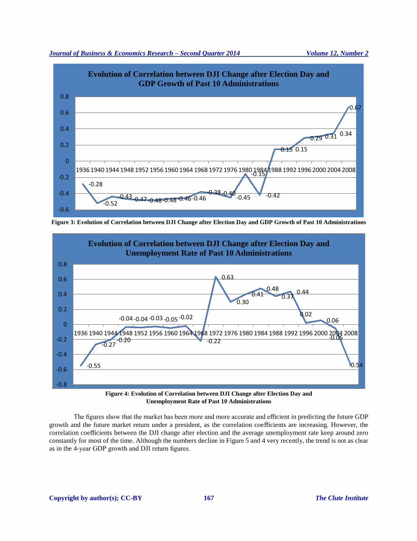
Figures 3, 4, and 5 show more information by presenting the evolution of historical correlations between DJI

change after Election Day and other indicators of interest. Figure 3 shows the evolution of correlation coefficients

between DJI change after Election Day and GDP growth. The calculation of correlation coefficients in Figure 3 is as

follows. For each observation, the value is the correlation coefficient of two time series data, each containing 10

numbers which indicate 10 administrations in past years - one is the DJI 1-Day Change from Table 1 and the other is

the Cumulative GDP Growth from Table 2. For example, the value of the observation in 1940 (equal to -0.52) is the

correlation coefficient of DJI 1-Day Change from 1904 to 1940 (for observation in 1972, it is from 1936 to 1972,

across 40 years and 10 administrations) and Cumulative GDP Growth during the same period. The higher value in

later years means the greater match between DJI change after Election Day and the cumulative GDP growth under the

president’s four-year administration.

The other figures are generated in a similar way. Figure 4 presents the evolution of correlation coefficients

between DJI changes after Election Day and the average unemployment rate, and Figure 5 presents the evolution of

correlation coefficients between DJI change after Election Day and the overall DJI return within four years.

0 1 2 3 4 5 6 7 8 9

10 11 12 13 14 15 16 17 18 19 20 21 22 23 24 25

19

01

19

05

19

09

19

13

19

17

19

21

19

25

19

29

19

33

19

37

19

41

19

45

19

49

19

53

19

57

19

61

19

65

19

69

19

73

19

77

19

81

19

85

19

89

19

93

19

97

20

01

20

05

20

09

Republican Unemployment

Unemployment Rate Over Time Under Each Party*



Figure 3: Evolution of Correlation between DJI Change after Election Day and GDP Growth of Past 10 Administrations

Figure 4: Evolution of Correlation between DJI Change after Election Day and

Unemployment Rate of Past 10 Administrations

The figures show that the market has been more and more accurate and efficient in predicting the future GDP

growth and the future market return under a president, as the correlation coefficients are increasing. However, the

correlation coefficients between the DJI change after election and the average unemployment rate keep around zero

constantly for most of the time. Although the numbers decline in Figure 5 and 4 very recently, the trend is not as clear

as in the 4-year GDP growth and DJI return figures.

-0.28

-0.52 -0.43 -0.47 -0.48 -0.48 -0.46 -0.46

-0.38 -0.40 -0.45

-0.15

-0.42

0.15 0.15

0.29 0.31 0.34

0.67

-0.6

-0.4

-0.2

0

0.2

0.4

0.6

0.8

1936 1940 1944 1948 1952 1956 1960 1964 1968 1972 1976 1980 1984 1988 1992 1996 2000 2004 2008

Evolution of Correlation between DJI Change after Election Day and

GDP Growth of Past 10 Administrations

-0.55

-0.27 -0.20

-0.04 -0.04 -0.03 -0.05 -0.02

-0.22

0.63

0.30 0.41

0.48 0.37

0.44

0.02 0.06

-0.05

-0.54

-0.8

-0.6

-0.4

-0.2

0

0.2

0.4

0.6

0.8

1936 1940 1944 1948 1952 1956 1960 1964 1968 1972 1976 1980 1984 1988 1992 1996 2000 2004 2008


Unemployment Rate of Past 10 Administrations



Figure 5: Evolution of Correlation between DJI Change after Election Day and

DJI Change for 4 Years of Past 10 Administrations

There is a possibility that the results are due to coincidence since the correlation analysis does not ensure the

causality, as most research has encountered similar problems; but each of stock market, economic indicators, and

presidential election attracts people’s attention and it is useful to show readers the important relationships between

them.

RESULTS

Table 4 shows six regressions of which (1), (2), and (5) show the results of a sub-sample of the most recent

ten administrations from Richard Nixon/Gerald Ford in 1972. Models (1) and (2) show that for the most recent ten

administrations, the 1-day DJI percentage change following the Election Day is a significant predictor of the

cumulative GDP growth of the following four years. However, Models (3) and (4) show that the prediction has no

significant accuracy when all 28 administrations since 1900 are included. Models (5) and (6) show that the 1-day DJI

percentage change following the Election Day and the average unemployment rate of the following four years has no

correlation in both the sub-sample and the full sample.

Table 4: Results of Regressions

Model (1) (2) (3) (4) (5) (6)

Cumulative

GDP

Growth

Cumulative

GDP

Growth

Cumulative

GDP

Growth

Cumulative

GDP

Growth

Average

Unemployment

Average

Unemployment

DJI 1-Day Change 1.660* 1.533* -0.677 -1.918 -0.385 -0.294

(0.699) (0.605) (1.798) (1.678) (0.214) (0.266)

Lag Cumulative

GDP Growth

-0.190

(0.431)

-0.334

(0.205)

Constant 14.35* 11.97*** 19.34*** 14.25*** 6.327*** 6.206***

(5.528) (1.166) (4.496) (3.325) (0.412) (0.528)

N 10 10 28 28 10 28

R2 0.460 0.446 0.139 0.048 0.288 0.045

Standard Errors In Parentheses, * p < 0.05, ** p < 0.01, *** p < 0.001

-0.59 -0.52 -0.52

-0.48 -0.43 -0.43 -0.42

-0.65 -0.62

-0.24

0.08 0.03

0.10

0.33

-0.04

0.16 0.21

0.11 0.04

-0.8

-0.6

-0.4

-0.2

0

0.2

0.4

1936 1940 1944 1948 1952 1956 1960 1964 1968 1972 1976 1980 1984 1988 1992 1996 2000 2004 2008


DJI Change for 4 Years of Past 10 Administrations



CONCLUSION

The authors’ study adds to the literature on examining the relationship between a presidential administration

and the economy. The researchers demonstrated that GDP growth is associated with the prediction of the Wall Street,

as defined by the change in stock price immediately after the election. This relationship has strengthened over time.

The researchers were not able to identify the same relationship between stock market change immediately after an

election and unemployment. The divergent results may be explained by the political economy framework and the

strong relationship between business and the presidential administration. Given that the focus of business is on growth

and not full employment, these results suggest that when Wall Street casts its prediction after an election, the

prediction focuses on growth and excludes unemployment variables. Additional research is needed to determine how

GDP, unemployment, and presidential policies interrelate.

AUTHOR INFORMATION

Wen-Wen Chien is an Assistant Professor of Accounting at State University of New York at Old Westbury. E-mail:

[email protected] (Corresponding author)

Roger W. Mayer is an Instructor at Walden University. E-mail: [email protected]

Zigan Wang is a PhD candidate in economics at Columbia University. E-mail: [email protected]

REFERENCES

1. Allvine, F. C., & O’Neil, D. E. (1980). Stock market returns and the presidential election cycle: Implications

for market efficiency. Financial Analysts Journal, 36, 49-56.

2. Barro, R. J. (1977). Unanticipated money growth and unemployment in the United States. The American

Economic Review, 67, 101-115.

3. Caro, R. (2002). The years of Lyndon Johnson: Master of the Senate. New York, NY: Alfred Knopf.

4. Darby, M. R. (1976). Three-and-a-half million U.S. Employees have been mislaid: Or, an explanation of

unemployment. Journal of Political Economy, 84, 1934-1941.

5. Fama, E. (1970). Efficient capital markets: A review of theory and empirical work. Journal of Finance, 25,

383-417.

6. Gilpin, R. (2001). Global political economy: Understanding the international economic order. Princeton,

NJ: Princeton University Press.

7. Goodell, J. W., & Bodey, R. A. (2012). Price-earnings changes during US presidential election cycles: Voter

uncertainty and other determinants. Public Choice, 150, 633-650.

8. Goodell, J. W., & Vähämaa, S. (2013). U.S. presidential elections and implied volatility: The role of political

uncertainty. Journal of Banking & Finance, 37, 1108–1117. Retrieved from

http://dx.doi.org/10.1016/j.jbankfin.2012.12.001

9. Huang, R. D. (1985). Common stock returns and presidential elections. Financial Analysts Journal, 41,

58-61.

10. Johnson, R. R., Chittenden, W. T., & Jensen, G. R. (1999). Presidential politics, stocks, bonds, bills, and

inflation. The Journal of Portfolio Management, 26, 27-31.

11. Jones, S. T., & Banning, K. (2009). U.S. elections and monthly returns. Journal of Economics and Finance,

33, 273-287.

12. Maddison, A. (2008). Historical statistics of the world economy: 1-2008 Ad, dataset. Retrieved from

http://rwanda.opendataforafrica.org/xpjarsb

13. Niederhoffer, V., Gibbs, S., & Bullock, J. (1970). Presidential elections and the stock market. Financial

Analysts Journal, 26, 111-113.

14. Riley, W. B., & Luksetich, W.A. (1980). The market prefers Republicans: Myth or reality. Journal of

Financial and Quantitative Analysis, 15, 541-560.

15. Romer, C. (1986). Spurious volatility in historical unemployment data. The Journal of Political Economy,

94, 1-37.

mailto:[email protected]





16. Santa-Clara, P., & Valkanov R. (2003). The presidential puzzle: Political cycles and the stock market. The

Journal of Finance, 58, 1841-1872.

17. U.S. Bureau of Labor Statistics. (2013). Labor force statistics from the current population survey. Retrieved

from http://data.bls.gov/pdq/SurveyOutputServlet

18. Wisniewski, T. P., Lightfoot, G., & Lilley, S. (2012). Speculating on presidential success: Exploring the link

between the price-earnings ratio and approval ratings. Journal of Economics and Finance, 36(1), 106-122.

Stock Market, Economic Performance, And Presidential ... · Roger W. Mayer, Walden University, USA...

Documents

Transcript of Stock Market, Economic Performance, And Presidential ... · Roger W. Mayer, Walden University, USA...