Stock market and the Stock market and the Economy: introductionEconomy: introductionThe purpose of this introduction is two-fold:

i. Introduce the concept of Expected Present Discounted Value, which is the foundation for IS/LM extensions;

ii. Distinguish between nominal & real interest rates and consider the impact that money growth has on these variables by extending the IS/LM model.

Expected Present Discounted Expected Present Discounted ValuesValues

The expected present value of a sequence of future payments is the value today of this expected sequence of payments.

In order to decide whether I make an investment, I compute the value today of the expected returns (benefits) of the investment and compare with the cost of investing.

If this value exceeds costs then I make the investment

If the one-year nominal interest rate is it lending $1 today yields $(1+ it) next year

Hence $1 next year is worth today ti+1

1$

ti+11

is the discount factor which is the present

discounted value of $1 next year.

The discount factor lies between zero and one since the discount rate (the nominal interest rate) iitt > 0 > 0

The higher the discount rate the lower the discount factor

Therefore $1 in two years time is worth $(1+it)(1+it+1)

and thus $1 two years from today must be worth

)1)(1(

1$

1+++ tt ii

• The present discounted value of a sequence of payments, or value in today’s dollars equals:

$ $( )

$( )( )

$V zi

zi i

zt tt

tt t

t= ++

++ +

+⋅⋅⋅++

+

11

11 11

12

where $zt is today’s payment; $zt+1 is the payment next year etc…

If $z t= $zt+1 =…..= $zt+n then

thus

$ $( ) ( )

V zi it t n= +

++⋅⋅⋅+

+⎡

⎣⎢

⎤

⎦⎥−1

11

11 1

$ $[ / ( ) ]

[ / ( )]V z

i

it t

n

=− +− +

1 1 11 1 1

Geometric series

We are interested in computing the expected present discounted value when future payments and interest rates are uncertain

This equation implies:1. Present value depends positively on today’s actual

payment and expected future payments

2. Present value depends negatively on current and expected future interest rates

$ $( )

$( )( )

$V zi

zi i

zt tt

et

te

t

et= +

++

+ ++⋅⋅⋅+

++

11

11 11

12

La formazione del prezzo di La formazione del prezzo di un’attività finanziaria:un’attività finanziaria:

il problema della allocazione delle risorse tra consumo e risparmio (investimento) per un individuo

obiettivo dell’individuo è distribuire il proprio consumo nel tempo in modo ottimale (massimizzando la propria utilità)

a tal fine l’individuo effettua transizioni in attività reali e finanziarie

Problema del consumatore:Problema del consumatore:

beneficio marginale di consumare un euro in beneficio marginale di consumare un euro in più oggipiù oggi==beneficio marginale di consumare domani un beneficio marginale di consumare domani un euro investito oggi in qualche attivitàeuro investito oggi in qualche attività(confrontare in ogni periodo l’utilità marginale che deriva da una unità di consumo aggiuntiva oggi con quella derivante dalla rinuncia a consumare quella unità aggiuntiva oggi per consumarla domani)

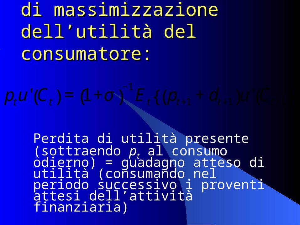
Soluzione del problema di Soluzione del problema di massimizzazione dell’utilità del massimizzazione dell’utilità del consumatore:consumatore:

Perdita di utilità presente (sottraendo pt al consumo odierno) = guadagno atteso di utilità (consumando nel periodo successivo i proventi attesi dell’attività finanziaria)€

ptu' Ct( ) = 1+σ( )−1

E t pt +1 + dt +1( )u' Ct +1( ){ }

Tasso di preferenza Tasso di preferenza intertemporale (intertemporale ():):

Δct+1

ct+1

ct

Δct

Curva di indifferenza intertemporale. Il valore assoluto della pendenza di una curva di indifferenza intertemporale in un punto è detto saggio marginale di preferenza intertemporale, cioè |Δct+1/Δct|.

Se la funzione di utilità del Se la funzione di utilità del consumatore è lineareconsumatore è lineare

l’utilità marginale sarà costante, cioè

€

u'(Ct ) = u' Ct +1( ) = u' C( )

Se l’attività finanziaria oggetto Se l’attività finanziaria oggetto dell’investimento del consumatore è dell’investimento del consumatore è un’azione, avremo:un’azione, avremo:pptt = v = vtt

dove dove vvtt indica il valore dell’azione, quindi indica il valore dell’azione, quindi

€

v t =E t v t +1 + dt +1( )

1+σ( )

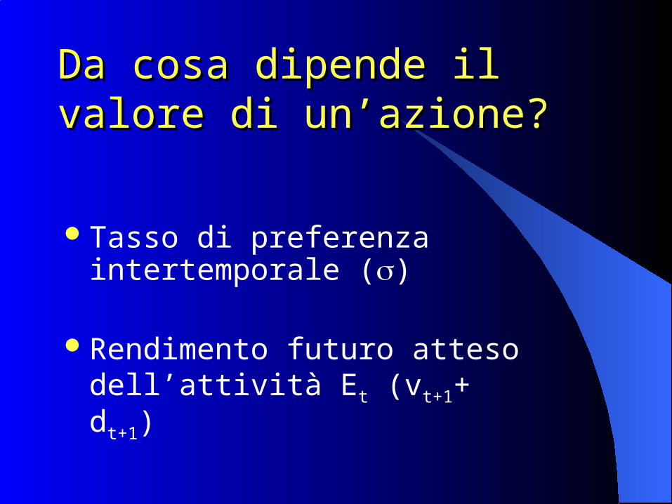
Da cosa dipende il valore di Da cosa dipende il valore di un’azione?un’azione?

Tasso di preferenza intertemporale ()

Rendimento futuro atteso dell’attività Et (vt+1+ dt+1)

La determinazione del coefficiente di La determinazione del coefficiente di attualizzazioneattualizzazione

Ipotesi: le attività più rischiose dovranno scontare i flussi di reddito attesi a tassi maggiori rispetto a quelli relativi ad attività meno volatili

Coefficiente di attualizzazione Coefficiente di attualizzazione (():):

doveirf = tasso di interesse risk-free r = premio per il rischio dell’attività

€

=irf + ρ

The components of an interest The components of an interest rate: the risk-free raterate: the risk-free rate The risk-free rate (denoted as irf) is approximately the yield on

short-term Treasury bills– Includes the pure rate and an allowance for inflation

Viewed as a conceptual floor for the structure of interest rates The Inflation Adjustment

– Inflation refers to a general increase in prices– Refers to the fact that, if prices rise, $100 at the beginning of the year

will not buy as much at the end of the year– If you loaned someone $100 at the beginning of the year, you need to

be compensated for what you expect inflation to be during the year Interest rates include estimates of average annual inflation over loan

periods

The components of an interest The components of an interest rate: risk premiumsrate: risk premiums Default risk: refers to the chance that the lender will not

receive the full amount of principal and interest payments agreed upon;

Liquidity risk: refers to the extra interest demanded by lenders as compensation for bearing liquidity risk (associated with being unable to sell the bond of an little known issuer);

Maturity risk: long-term bond prices change more with interest rate swings than short-term bond price. Gives rise to maturity risk (investors demand a maturity risk premium ranging from 0% to 2% or more for long-term issues).

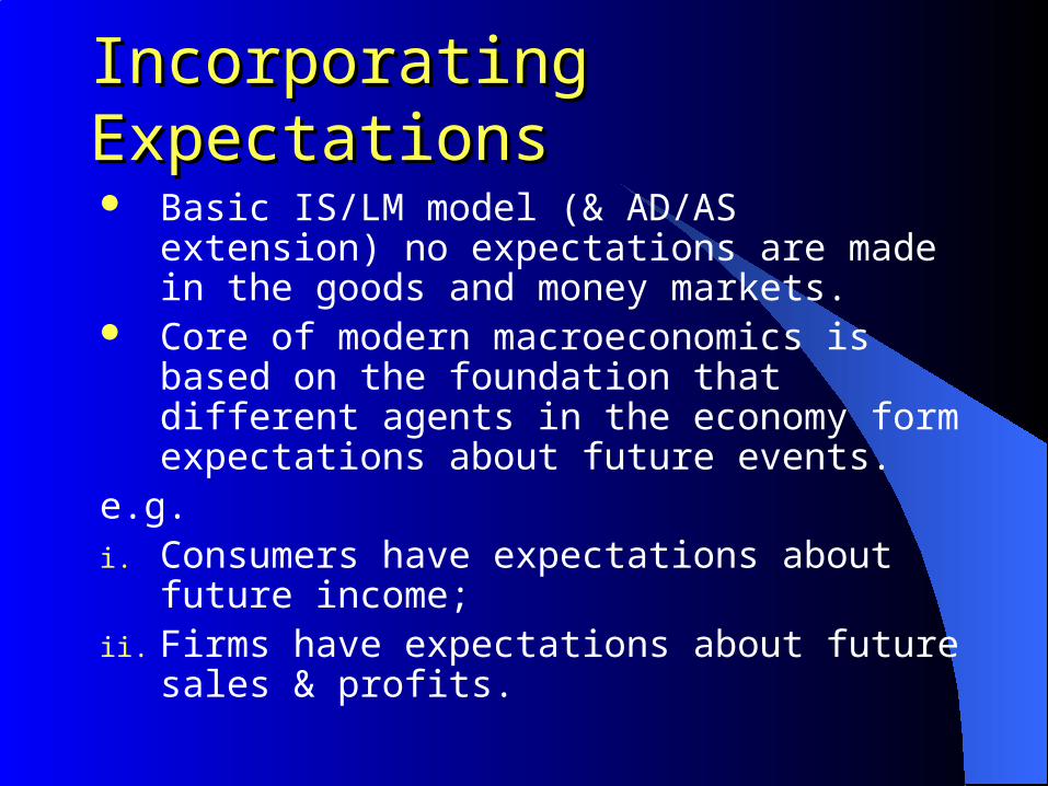
Incorporating ExpectationsIncorporating Expectations

Basic IS/LM model (& AD/AS extension) no expectations are made in the goods and money markets.

Core of modern macroeconomics is based on the foundation that different agents in the economy form expectations about future events.

e.g.i. Consumers have expectations about future

income;ii. Firms have expectations about future sales &

profits.

Stock market and the economy: outline

Distinguish between nominal and real interest rates (IS curve);

Consider the role of expectations in financial markets in the determination of bond and stock prices (LM curve);

Consider the role of expectations in consumption and investment decisions (IS curve)

Therefore our aim is to modify the basic IS/LM model (& AD/AS extension) to examine how fluctuations in economic conditions and macroeconomic policy may account for movements in the stock market.

Nominal vs Real Interest Nominal vs Real Interest RatesRates Nominal Interest Rate is the interest rate

expressed in units of money (it) It tells us how much money we have to pay in the

future in exchange for having one more unit of money today (1+it )

Real Interest Rate is the interest rate expressed in terms of a basket of goods (rt)

It tells us how many goods we have to give up in the future in exchange for having one more basket of goods today (1+it )

The Real Interest Rate is important since agents consume goods and not money!

Deriving the Real Interest Deriving the Real Interest RateRate Borrow money today to buy a good of price Pt then

you have to repay (1+it ) Pt next year In terms of the good you have to repay

where PPeet+1 t+1 denotes the price expectation of the good denotes the price expectation of the good

next year.next year.

Therefore it follows that the one-year real interest Therefore it follows that the one-year real interest rate israte is

et

Pt)Pti(

tr1

11

+

+=+

et

Pt)Pti(

1

1

+

+

Therefore Therefore

π et

et t

t

P P

P≡

−+1

( )11

1+ =

++

ri

ttetπ

Expected inflation is defined asExpected inflation is defined as

Note that:Note that:

r it te

t= −π

Thus the real interest rate is (approximately) equal to the Thus the real interest rate is (approximately) equal to the nominal interest rate minus the expected rate of inflation.nominal interest rate minus the expected rate of inflation.

)1()1(

)1( ettie

tti ππ −+≈

++

Fisher equation

provided πet & it are small

r it te

t= −π Implications of the Fisher Equation:

trtiet =⇒= ;0π

trtiet >⇒> ;0π

0; =⇒= trtietπ

treti ↓↑ ,; π

Nominal and Real Interest Nominal and Real Interest Rates in the United States Rates in the United States Since 1978Since 1978

Nominal and Real One-Year T-bill Rates in the United States, 1978-2001

While the nominal interest rate has declined considerably since the early 1980s, the real interest rate is actually higher in 2001 than it was then.

Nominal & Real Interest Rates & the Nominal & Real Interest Rates & the IS/LM ModelIS/LM Model So far you have encountered the following version of the

IS curve:

Y=C(Y-T)+I(Y,i)+G

• Here investment depends on the nominal interest rate.

• However since firms produce goods, their investment decision should depend on how many goods they have to repay (and not how much money).

• Therefore investment spending depends on the real interest rate and the modified IS curve is

Y=C(Y-T)+I(Y,r)+G

Modified IS/LM modelModified IS/LM model

IS: Y = C(Y-T)+I(Y,i-πe)+G

LM: M/P = YL(i)

Money market equilibrium (LM curve) still depends on the nominal interest rate, since the opportunity cost of holding money is the rate of return from holding bonds ii

Goods market equilibrium now also depends on πe

Equilibrium Output and Interest Rates

The equilibrium level of output and the equilibrium nominal interest rate are given by the intersection of the IS curve and the LM curve. The real interest rate equals the nominal interest rate minus expected inflation.

If r = i - πe, then ∆r = ∆ i - ∆ πe, and if πe is constant then ∆ πe = 0 and ∆r = ∆ i.

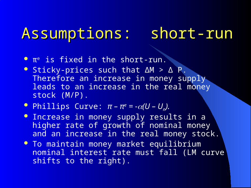
Assumptions: short-runAssumptions: short-run

πe is fixed in the short-run. Sticky-prices such that ∆M > ∆ P. Therefore an increase

in money supply leads to an increase in the real money stock (M/P).

Phillips Curve: π – πe = -(U – Un). Increase in money supply results in a higher rate of

growth of nominal money and an increase in the real money stock.

To maintain money market equilibrium nominal interest rate must fall (LM curve shifts to the right).

The Short-run Effects of an Increase in Money Growth

An increase in money growth increases the real money stock in the short run. This increase in real money leads to an increase in output and a decrease in both the nominal and the real interest rate.

Output increases as the nominal interest rate falls. IS curve does not shift since πe is fixed. The increase in output results in a fall in

unemployment below its natural rate. From the Phillips Curve this implies that inflation increases.

The Fisher equation is

Thus the real interest rate must fall with the nominal interest rate.

Thus higher money growth leads to lower nominal interest rates and lower real interest rates in the short-run.

r it te

t= −π

Medium-RunMedium-Run

πe = π (expected inflation = actual inflation) Phillips Curve: π – πe = 0 = - (U – Un). Thus,

unemployment remains at is natural rate. Output remains at its natural rate

and thus the real interest rate is unaffected. The Quantity Theory of Money holds such that π

= gm (inflation = money growth rate) assuming for simplicity that the rate of growth of output equals zero.

Fisher equation: i = r + πe = r + π = r + gm In the medium-run, an increase in money growth

leads to an equal increase in the nominal interest rate. The real interest rate is unchanged.

Y C Y T I Y r Gn n n= − + +( ) ( , )

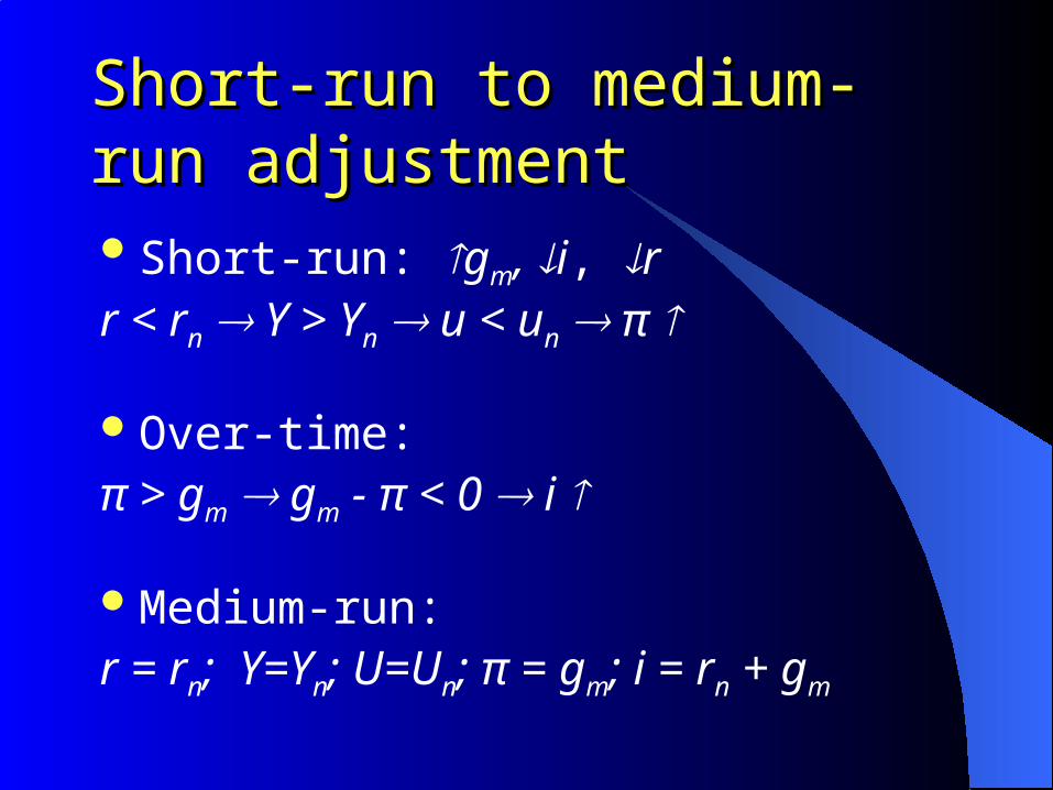
Short-run to medium-run Short-run to medium-run adjustmentadjustmentShort-run: gm, i, rr < rn Y > Yn u < un π

Over-time:π > gm gm - π < 0 i

Medium-run:r = rn; Y=Yn; U=Un; π = gm; i = rn + gm

Fisher HypothesisFisher Hypothesis

To summarize, in the medium run money growth does not affect the real interest rate, but the nominal interest rate increases one for one with inflation. This result is known as the Fisher effect, or the Fisher Hypothesis.

This hypothesis is important for two reasons.1. In offers a testable theory in explaining changes in

interest rates.

2. The Fisher Hypothesis supports the Quantity Theory of Money, i.e. money is neutral in the medium run.

Evidence on the Fisher Evidence on the Fisher HypothesisHypothesis To see if increases in inflation lead to one-for-

one increases in nominal interest rates, economists look at:

1. Nominal interest rates and inflation across countries. The evidence of the early 1990s finds substantial support for the Fisher hypothesis

2. Swings in inflation, which should eventually be reflected in similar swings in the nominal interest rate. Again, the data appears to fit the hypothesis quite well

This offers further support that monetary policy should primarily be used to maintain low and stable inflation

Evidence on the Fisher Evidence on the Fisher HypothesisHypothesis

Nominal Interest Rates and Inflation Across Latin America in the Early 1990s

Roughly half of the points are above the line, the other half below. This is evidence that a 1% increase in inflation should be reflected in a 1% increase in the nominal interest rate.

Evidence on the Fisher Evidence on the Fisher HypothesisHypothesis

The Three-Month Treasury Bill Rate and Inflation, 1927-2000

The increase in inflation from the early 1960s to the early 1980s was associated with an increase in the nominal interest rate. The decrease in inflation since the mid-1980s has been associated with a decrease in the nominal interest rate.

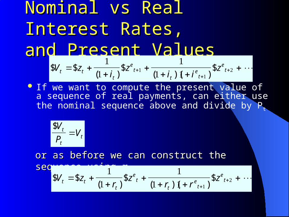
Nominal vs Real Interest Rates,Nominal vs Real Interest Rates,and Present Valuesand Present Values

If we want to compute the present value of a sequence of real payments, can either use the nominal sequence above and divide by Pt

or as before we can construct the sequence using ror as before we can construct the sequence using r tt

$ $( )

$( )( )

$V zi

zi i

zt tt

et

te

t

et= +

++

+ ++⋅⋅⋅+

++

11

11 11

12

$ $( )

$( )( )

$V zr

zr r

zt tt

et

te

t

et= +

++

+ ++⋅⋅⋅

++

11

11 1 1

2

$V

PVt

tt=

We have two formula’s for computing the present value of sequence of payments:

1. Based on nominal interest rate which we will use when considering the pricing of financial assets. Why? Since bonds offer nominal returns.

2. Based on real interest rate which we will use in considering consumption and investment decisions. Why? Base expectations on future real income.

Where do we go from here?Where do we go from here?

We will consider the role of expectations in determining bond and stock prices using are present value formula.

Derive the yield curve used to predict the future short-term interest rate

Consider the relationship between economic activity and stock prices

Speculative bubbles in the stock market