Stochastic simulations of fault networks in 3D

structural modeling∗

Nicolas Cherpeau 12, Guillaume Caumon 2and Bruno Levy 3

Abstract

3D Structural modeling is a major instrument in geosciences, e.g.for the assessment of groundwater and energy resources or nuclearwaste underground storage. Fault network modeling is a particularlycrucial step during this task, for faults compartmentalize rock units andplay a key role in subsurface flow, whether faults are sealing barriersor drains.

Whereas most structural uncertainty modeling techniques only al-low for geometrical changes and keep the topology fixed, we proposea new method for creating realistic stochastic fault networks with dif-ferent topologies. The idea is to combine an implicit representation ofgeological surfaces which provides new perspectives for handling topo-logical changes with a stochastic binary tree to represent the spatialregions. Each node of the tree is a fault, separating the space in twofault blocks. Changes in this binary tree modify the fault relations andtherefore the topology of the model.

Resume

Simulations stochastiques de reseaux de failles en modelisationstructurale 3D. La modelisation structurale est largement utilisee engeoscience, notamment pour l’evaluation des ressources energetiqueset hydriques du sous-sol. La caracterisation des failles est l’une desetapes cles du processus de modelisation etant donne leur importancedans les ecoulements de subsurface.

Alors que la plupart des techniques de modelisation d’incertitudesstructurales existantes perturbent seulement la geometrie des objets,nous proposons une nouvelle methode de simulation stochastique dereseaux de failles, incluant des changements topologiques. Cette methode

∗Published in Comptes Rendus Geoscience, 342(9):687 – 694, 2010. ISSN 1631-0713.doi : 10.1016/j.crte.2010.04.008.

1e-mail: nicolas.cherpeau@gocad.org2Centre de Recherches Petrographiques et Geochimiques - Universite Lorraine, Ecole

Nationale Superieure de Geologie, Rue du doyen Marcel Roubault, 54501 Vandoeuvre-les-Nancy, France

3Centre INRIA Nancy Grand-Est, Campus scientifique, 615 rue du Jardin Botanique,54600 Villers les Nancy, France

1

associe une modelisation implicite des surfaces geologiques, avec unarbre binaire permettant d’agencer les regions spatiales du modele.Chaque noeud de l’arbre represente une faille, separant l’espace endeux blocs. Des changements dans l’arbre binaire modifient les rela-tions entre failles et par consequent la topologie du modele.

KEYWORDS3D structural modeling; Structural uncertainties; Implicit modeling;Fault network; Constructive Solid Modeling

Mots cles : Modelisation structurale 3D, Incertitudes structurales,Modelisation implicite, Reseau de failles, Modelisation solide

1 Introduction

A 3D structural model of the subsurface helps visualizing, understanding andquantifying geophysical processes and assessing natural resources. Indeed,geological structures control to some extend the spatial layout of subsur-face heterogeneities. Therefore, most geostatistical petrophysical modelingmethods use distances which follow folded and faulted structures [1, 2, 3].Moreover, physical modeling codes are best run on grids conforming to ge-ological structures [4, 5, 6].

However, surface geology and borehole data only provide limited infor-mation about subsurface structures and even exhaustively sampled 3D seis-mic surveys cannot remove interpretational uncertainties. Uncertainties aredue to the inherent incompleteness and the limited resolution of geologicaldata sets. Geology is by nature an interpretive science [7] and geologicalconcepts and physical laws help geoscientists reducing uncertainties. How-ever, geoscientists may introduce a prior geological knowledge bias and/orhuman bias [8] when interpreting subsurface data.

These uncertainties have a wide range of consequences in quantitativegeosciences, and Gilbert [9] and Chamberlin [10] in their pioneering workalready argued for multiple hypotheses. Consequently, uncertainties can beassessed by considering not just one (probably wrong) deterministic model,but a set of possible structural models. Depending on the amount and qual-ity of observations, three levels of uncertainty can be defined by comparingsuch possible 3D structural models:

• Low uncertainty when all models have the same layout of structuralsurfaces, and show relatively small geometric variations.

• Medium uncertainty when the geometry of surfaces changes more sig-nificantly and the connection between geological surfaces may varylocally.

2

• High uncertainty when the number of structural interfaces, their spa-tial layout and their geometry are globally variable, except at someobservation points.

From a modeling standpoint, these three degrees of uncertainty corre-spond to increasing difficulty. Therefore, multi-realization methods havemostly focused on low and medium uncertainty, primarily to assess riskin hydrocarbon reservoir management (rock volume estimates [11], under-ground flow [12], well plannning [13], history matching [14]). Most of thesemethods proceed by perturbing a reference interpretation to generate alarge number of equiprobable geometric models of geological structures. Infaulted formations, this may tend to underestimate variability by perturbingonly fault geometry and leaving the first-order fault connectivity constant.Therefore, existing methods are best suited for large scale studies (pluri-decametric) with high-resolution 3D seismic data. For smaller objects orsparser data, stochastic approaches should also sample large uncertaintieswhen generating possible models, some of which should be falsified whenevera new observation is made [15].

In this paper, we propose to sample both the connectivity and the ge-ometry of fault networks in order to account for large uncertainties due tolimited data quantity and resolution. Faults indeed are key elements in3D structural models, and often have a first-order impact on the modelingoutput.

After a review of uncertainty modeling methods using both traditionalexplicit modeling or recent implicit approach (section 2), we introduce ourstochastic fault simulation method (section 3).

2 Structural uncertainties: state of the art

Most existing structural uncertainty modeling methods proceed by perturb-ing a reference interpretation. The result is a large number of equiprobablegeometries representing the uncertainty relative to geological structures.

2.1 Explicit geometrical perturbation techniques and limita-tions

In explicit modeling, geological interfaces are represented as polygonal sur-faces. Lecour et al. [16] propose to modify the geometry of a surface byperturbing its nodes along an uncertainty bar defined at each node. The per-turbation is correlated along the surface using the probability field method[17], in order to obtain realistic geometries. In the case of fault perturba-tion, curvature sign along the sliding direction is preserved to ensure faultcompliance.

3

Figure 1: Topology changes induced by geometrical changes. In thereference case, the horizon H is in between faults F1 and F2. A simple driftof H along uncertainty vectors may completely change the configuration: Hcould possibly occur on either side of F1 or F2 and not anymore in betweenthe two faults.

Fig. 1. Changements topologiques induits par des perturbationsgeometriques. Dans le cas initial, l’horizon H se situe entre les failles F1

et F2. Une simple translation de H le long de vecteurs d’incertitude peutcompletement changer la configuration : H pourrait etre en contact avecseulement F1 ou F2 et ne plus se situer entre les deux failles.

Other techniques have been developed to perturb the geometry of struc-tural models, keeping the topology fixed [18, 19, 20, 14]. For a whole model,each surface is perturbed according to its structural uncertainties and allconnections (horizon to horizon, horizon to fault and fault to fault) arestored. Once all geological objects have been perturbed, connections arehonored so that the topology is preserved [16]. In practice, this raises anumber of challenges to maintain model consistency in the case of largeuncertainties, for interferences between surfaces and large mesh distorsionsmay occur. Moreover, large geometrical uncertainties may require topologychanges, for instance horizon to fault connections (Fig. 1).

2.2 Topological perturbation

Topology is all about connections and relations between objects. In a struc-tural model, topological changes may be introduced in different manners:

• Adding or removing geological objects.

4

• In the case of faults, changing the truncation rule between two faults.

• During geometrical perturbations, a simple drift of an horizon alonguncertainty vectors may induce a topological change (especially faultto horizon connections, Fig. 1).

Few methods have been proposed to change the topology of a structuralmodel. A fault modeling tool, referred to as Havana has been proposed in[21, 22]. It is mainly designed for the oil industry and works directly on acorner-point reservoir grid used for flow simulations. This choice allows fordirectly observing the effects of structural uncertainties on flow simulations.However, resevoir grids have known shortcomings to accurately representgeological structures. Consequently, sub-seismic faults are added by simplymodifying the permeability field. Main faults are bilinear planes parallel tothe pillars of the reservoir grid or stair-stepped faults.

In our approach, we borrow the idea of fault operator to [21], but usea flexible representation of faults. This makes it possible to account forlarge structural uncertainties without making simplifications due to the gridorientation. For accuracy, this method uses an implicit representation ofstructural interfaces, as in [23, 24, 25].

2.3 Implicit modeling: new perspectives for 3D modeling

An implicit surface (e.g. Fig. 3d) is described by an isovalue f of a mono-tonic volumetric function F(x, y, z) (e.g. Fig. 3a,c)(e.g. the geological time[26], the signed distance to an object [27]):

F(x, y, z) = f (1)

A conforming stratigraphic column is then represented as a set of isopo-tentials of a same scalar field, whereas unconformities and faults are definedby their own scalar field. Consequently, horizons can be perturbed indepen-dently of faults. Truncations by faults are only honored when an explicitsurface is extracted from an isovalue of a scalar field.

Implicit modeling provides a means to easily truncate some surfaces byothers using Constructive Solid Geometry (CSG) concepts. For instance, asurface A (FA(x, y, z) = fA) can be truncated by another implicit surface B(FB(x, y, z) = fB), by making a boolean intersection between A and eitherhalf-spaces of B (Fig. 2). For instance, a truncated surface A|B+ is definedby:

FA(x, y, z) = fA|FB(x, y, z) ≥ fB (2)

The reference scalar field of an implicit surface (F(x, y, z) = f) can beperturbed by introducing a correlated random field R(x, y, z) [18]. The newsurface is defined by the same isovalue f in the field F(x, y, z) +R(x, y, z)(Fig. 3).

5

fbfa

fa

+ →

a.

b. c.

fa

fb

A-

+

A

+- B

∩

A+ -B∩

A+

B

+B

∩A- -B∩A- +B

→

→

→

→→

Figure 2: Boolean operations in implicit modeling. a. Left: twosurfaces A (FA(x, y, z) = fA) and B (FB(x, y, z) = fB) and theircorresponding half-spaces. Right: boolean sum of the two scalarfields defining four spatial regions. b. Example of boolean operation:FA(x, y, z) ∩ FB(x, y, z) ≥ fB. c. Example of truncation corresponding tothe operation: FA(x, y, z) = fA ∩ FB(x, y, z) ≥ fB (equation 2).

Fig 2. Operations booleennes en modelisation implicite. a. Gauche : deuxsurfaces A (FA(x, y, z) = fA) et B (FB(x, y, z) = fB) et leurs demi-espaces.Droite: 4 regions spatiales definies par l’intersection des deux champsscalaires. b. Exemple d’operation booleenne: FA(x, y, z)∩FB(x, y, z) ≥ fB.c. Exemple d’intersection : FA(x, y, z) = fA ∩ FB(x, y, z) ≥ fB (equation2).

3 A new method for stochastic simulations of faultnetworks

The proposed stochastic fault simulation method takes advantage of the im-plicit surface perturbation and CSG operations between faults. To representhow faults partition the domain and interact one with another, we proposeusing a binary tree.

3.1 Binary trees as descriptors of fault relationships

Indeed, each fault divides the modelM in two distinct fault blocks B− andB+ [28], defined by:

• B− = {(x, y, z) ∈M|F(x, y, z) < f}

• B+ = {(x, y, z) ∈M|F(x, y, z) > f}

6

Figure 3: Geometrical perturbation method in implicit modeling. a. Thereference scalar field F(x, y, z) defining the initial implicit surface (isovaluef , planar surface). b. A correlated random field R(x, y, z) generated bySequential Gaussian Simulation represents the perturbation field. c. Thesurface is now defined by the isovalue f in the field F(x, y, z) +R(x, y, z).d. View of the perturbed surface.

Fig 3. Methode de perturbation geometrique en modelisation im-plicite. a. Le champ scalaire de reference F(x, y, z) definit la surface initiale(isovaleur f , surface plane). b. Un champ aleatoire correle genere par uneSimulation Sequentielle Gaussienne correspond au champ de perturbation.c. La surface est maintenant definie par l’isovaleur f dans le champF(x, y, z) +R(x, y, z). d. Surface perturbee.

Then, in the binary tree representing a fault network, each node representsa fault and each leave (node without children) represents a fault block (Fig.4).

Each fault in the tree is potentially a branching fault for its parentfaults in the tree. Switching a parent and its child in the tree changes theirrelationship: the main fault becomes the branching fault and inversely (Fig.5). A special case may occur when a fault F cuts a set of older faultsSold = {Fi|i ∈ [1, n]}. In this case, the oldest faults Sold are on both sides of

7

Figure 4: A fault network and its topological representation as a binarytree. a. Fault network in 3D. b. The same model in top view to make thetopology more explicit. Each fault Fi divides the model in two blocks Bi.c. Binary tree representing the fault relationships. The fault F4 is the mainand oldest fault (root node of the tree), other faults are branching faults.

Fig. 4. Un reseau de failles et sa representation topologique en ar-bre binaire. a. Reseau de failles en 3D. b. Le meme modele vu de dessusafin d’expliciter la topologie. Chaque faille Fi coupe le modele en deuxblocs Bi. c. Arbre binaire representant les relations entre failles. La failleF4 est la faille principale (racine de l’arbre), les autres failles etant desfailles secondaires.

the cutting fault F in the 3D model, hence they appear in the two branchesof F in the tree (Fig. 5c).

When modeling a given fault array, some faults may not be truncatedby other faults. Therefore, individual faults can be considered either parentor child in the binary tree, there is no consequence in term of truncationsince faults are not in contact. Consequently, a given fault network maybe described by several binary trees (Fig. 6). As there is no one-to-one

8

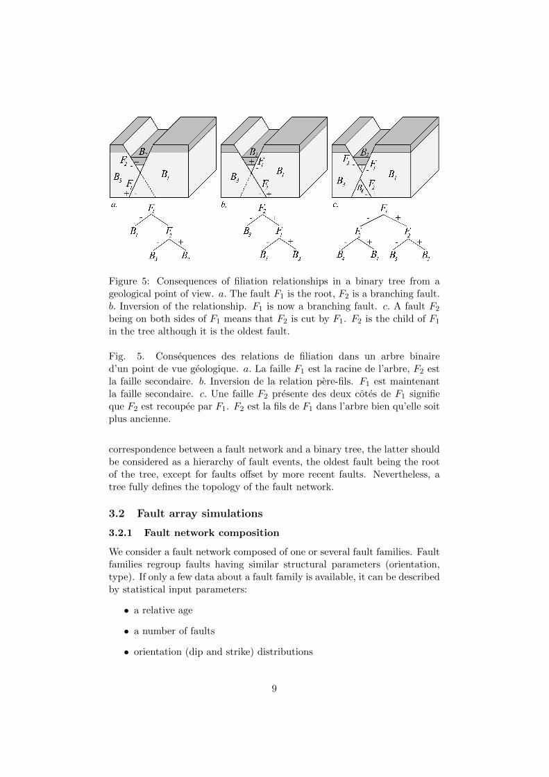
Figure 5: Consequences of filiation relationships in a binary tree from ageological point of view. a. The fault F1 is the root, F2 is a branching fault.b. Inversion of the relationship. F1 is now a branching fault. c. A fault F2

being on both sides of F1 means that F2 is cut by F1. F2 is the child of F1

in the tree although it is the oldest fault.

Fig. 5. Consequences des relations de filiation dans un arbre binaired’un point de vue geologique. a. La faille F1 est la racine de l’arbre, F2 estla faille secondaire. b. Inversion de la relation pere-fils. F1 est maintenantla faille secondaire. c. Une faille F2 presente des deux cotes de F1 signifieque F2 est recoupee par F1. F2 est la fils de F1 dans l’arbre bien qu’elle soitplus ancienne.

correspondence between a fault network and a binary tree, the latter shouldbe considered as a hierarchy of fault events, the oldest fault being the rootof the tree, except for faults offset by more recent faults. Nevertheless, atree fully defines the topology of the fault network.

3.2 Fault array simulations

3.2.1 Fault network composition

We consider a fault network composed of one or several fault families. Faultfamilies regroup faults having similar structural parameters (orientation,type). If only a few data about a fault family is available, it can be describedby statistical input parameters:

• a relative age

• a number of faults

• orientation (dip and strike) distributions

9

Figure 6: Non uniqueness of the representation of a fault array in a binarytree. a. 3D diagram representing three faults. The faults F1 and F2 arenot in contact so they can either be parent or child in the binary tree. b.Representation of the three faults in a binary tree with F1 as the parentfault. c. F2 is now the root of the tree without any change about theirtruncation in the diagram. There may be a consequence of the changedeeper, outside the diagram.

Fig. 6. Non unicite de la representation d’un ensemble de faillesdans un arbre binaire. a. Diagramme 3D representant 3 failles. Les faillesF1 et F2 ne sont pas en contact. Par consequent, elles peuvent etre pereou fils dans l’arbre binaire. b. Arbre binaire avec F1 en tant que failleparente. c. F2 est maintenant la racine de l’arbre mais aucun recoupementn’a change. Il se peut que le recoupement change plus en profondeur, endehors du diagramme.

• perturbation parameters

Alternatively, fault families may be described by any scalar field (e.g.coming from the interpolation of field, borehole or seismic data) and per-turbation parameters defining the associated uncertainties. The key inputparameter is the relative age of faults since it determines the order of simu-lation and thus the place in the binary tree (section 3.2.3).

To simulate a fault array, only one binary tree is needed, containing allthe faults of the network. Different fault networks are obtained by generatingdifferent binary trees.

10

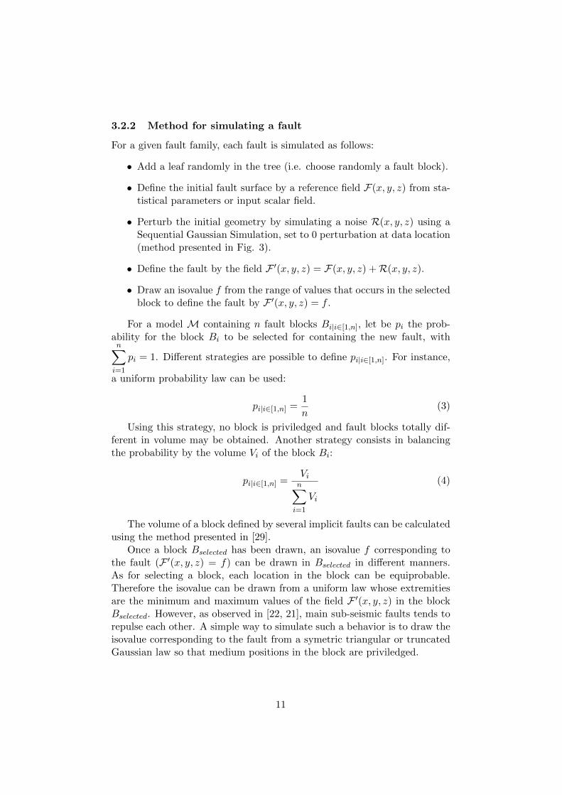
3.2.2 Method for simulating a fault

For a given fault family, each fault is simulated as follows:

• Add a leaf randomly in the tree (i.e. choose randomly a fault block).

• Define the initial fault surface by a reference field F(x, y, z) from sta-tistical parameters or input scalar field.

• Perturb the initial geometry by simulating a noise R(x, y, z) using aSequential Gaussian Simulation, set to 0 perturbation at data location(method presented in Fig. 3).

• Define the fault by the field F ′(x, y, z) = F(x, y, z) +R(x, y, z).

• Draw an isovalue f from the range of values that occurs in the selectedblock to define the fault by F ′(x, y, z) = f .

For a model M containing n fault blocks Bi|i∈[1,n], let be pi the prob-ability for the block Bi to be selected for containing the new fault, withn∑

i=1

pi = 1. Different strategies are possible to define pi|i∈[1,n]. For instance,

a uniform probability law can be used:

pi|i∈[1,n] =1

n(3)

Using this strategy, no block is priviledged and fault blocks totally dif-ferent in volume may be obtained. Another strategy consists in balancingthe probability by the volume Vi of the block Bi:

pi|i∈[1,n] =Vin∑

i=1

Vi

(4)

The volume of a block defined by several implicit faults can be calculatedusing the method presented in [29].

Once a block Bselected has been drawn, an isovalue f corresponding tothe fault (F ′(x, y, z) = f) can be drawn in Bselected in different manners.As for selecting a block, each location in the block can be equiprobable.Therefore the isovalue can be drawn from a uniform law whose extremitiesare the minimum and maximum values of the field F ′(x, y, z) in the blockBselected. However, as observed in [22, 21], main sub-seismic faults tends torepulse each other. A simple way to simulate such a behavior is to draw theisovalue corresponding to the fault from a symetric triangular or truncatedGaussian law so that medium positions in the block are priviledged.

11

3.2.3 Order of simulation

In the general case, fault families are simulated in chronological order, theoldest one first. Consequently, all the faults belonging to the same familyare branching faults for the faults belonging to older families (Fig. 7).

3.2.4 Case of cogenetic faulting

Faults with different structural characteristics (i.e., belonging to differentfamilies) may initiate simultaneously at the geological time scale and thustruncate each other. One example of such a situation are conjugate faults,corresponding to steeply opposed-dipping faults. In this case, fault familiescannot be simulated one after the other. Instead, let be Scoeval the set ofall the faults to be simulated belonging to cogenetic families. The methodis iterative: a fault is drawn in the set Scoeval and added randomly in thebinary tree, until Scoeval is empty. Consequently, faults belonging to a givenfamily may be parent or child for the other cogenetic families, hence differenttruncation rules between families (Fig. 8d).

3.2.5 Case of cross-cutting faults

A special situation may occur when a fault is offset by other faults (Fig.5c). Indeed, in this case, the parent fault in the tree is the youngest one.This situation can be obtained by simulating the youngest fault Fyoung

(Fyoung(x, y, z) = fyoung) first and then simulating the shifted fault Fshifted

in a block (adding it at one leaf as usually). Then, depending on the dis-placement of the cutting fault Fyoung, Fshifted may be added to anotherleaf. Assuming no rotation of Fyoung’s displacement, Fshifted is defined bythe same scalar field but by different isovalues depending on the fault block:

• Fshifted(x, y, z) = f−|Fyoung(x, y, z) ≤ fyoung

• Fshifted(x, y, z) = f+|Fyoung(x, y, z) ≥ fyoung

4 Perspectives and conclusion

We have introduced a new framework for modeling structural uncertainties.In particular, the method goes beyond the perturbation of deterministic 3Dstructural interpretations, but considers the uncertainty about connectivitiesbetween structural interfaces (Fig. 8). We expect this method to provide abasis for further advances in subsurface uncertainty management, including:

• Taking into account additional data, e.g. field and seismic data, sizedistribution, slip information. In the case seismic data is available,the global vertical displacement is known for the fault zone. The sumof the simulated displacement for all the faults present laterally in

12

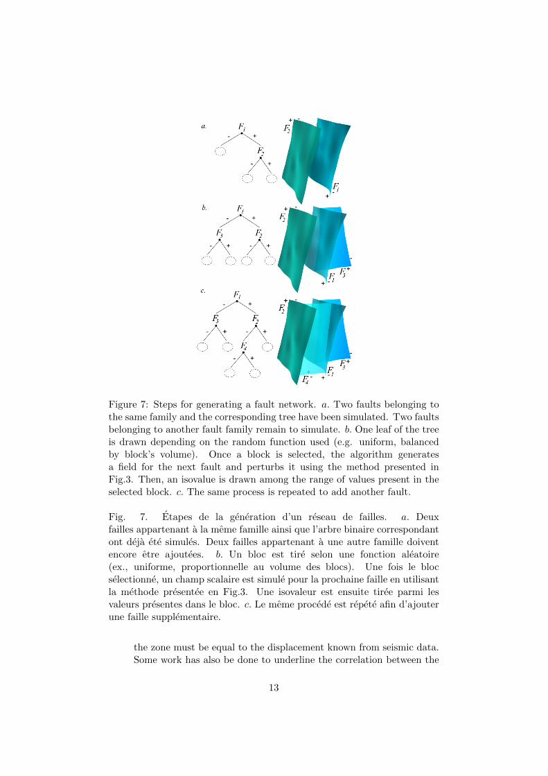
Figure 7: Steps for generating a fault network. a. Two faults belonging tothe same family and the corresponding tree have been simulated. Two faultsbelonging to another fault family remain to simulate. b. One leaf of the treeis drawn depending on the random function used (e.g. uniform, balancedby block’s volume). Once a block is selected, the algorithm generatesa field for the next fault and perturbs it using the method presented inFig.3. Then, an isovalue is drawn among the range of values present in theselected block. c. The same process is repeated to add another fault.

Fig. 7. Etapes de la generation d’un reseau de failles. a. Deuxfailles appartenant a la meme famille ainsi que l’arbre binaire correspondantont deja ete simules. Deux failles appartenant a une autre famille doiventencore etre ajoutees. b. Un bloc est tire selon une fonction aleatoire(ex., uniforme, proportionnelle au volume des blocs). Une fois le blocselectionne, un champ scalaire est simule pour la prochaine faille en utilisantla methode presentee en Fig.3. Une isovaleur est ensuite tiree parmi lesvaleurs presentes dans le bloc. c. Le meme procede est repete afin d’ajouterune faille supplementaire.

the zone must be equal to the displacement known from seismic data.Some work has also be done to underline the correlation between the

13

displacement of a fault and its size [30, 31]. Such correlations couldbe used either to simulate the displacement or laterally dying andsynsedimentary faults, depending on the available data.

• How to model particular fault zones? Using our method, realisticfault arrays are obtained but not particular configurations. One maywant to simulate, e.g. a fault relay zone, for there are evidence such astructure occurs in the studied area although uncertainties remain. Forinstance, the probability of a breaching fault to connect two segmentsof a relay zone must only be defined for the block in between the twosegments. It means that some blocks cannot be selected during thesimulation, i.e. the binary tree structure is constrained.

• Flower structures between two faults is another challenge since in thiscase, each fault is both parent and child of the other fault, corre-sponding to cycles in the tree. To solve this problem, the geometryof a flower structure may be obtained by considering one main faultdepending on the sliding direction and an inactive lentil bounded tothe sliding surface [32].

The method takes advantage of implicit modeling for both topology de-scription and changes. Each fault is fully described by a monotonic vol-umetric function F ′(x, y, z) corresponding to the sum of a reference fieldF(x, y, z), computed from statistical or hard data, and a spatially corre-lated random field R(x, y, z) corresponding to the associated uncertainties.We believe this implicit representation provides a convenient and robust wayof guaranteeing the model consistency.

A binary tree has been introduced to describe the spatial relationshipsbetween faults. The tree should be considered as a descriptor of fault events,a fault being a branching fault for its ascending branch in the tree. Duringthe fault simulation, faults are added in the tree according to their relativeage in order to obtain a fault network honoring input structural constraints.Fault arrays with different topologies are obtained by simulating differentbinary trees.

Such a multi-realization approach enables to assess the inherent uncer-tainties to geological data sets. Existing methods are mostly used in theoil industry to reduce economical risks. However, we believe it has a strongpotential in other application fields such as potential field interpretation orseismic waveform inversion.

Acknowledgements

This research was performed in the frame of the gOcad research project. Thecompanies and universities members of the gOcad consortium are acknowl-

14

edged for their support, as well as Paradigm Geophysical for also providingthe Gocad software and API. This is CRPG contribution 2020.

References

[1] J.-P. Chiles, P. Delfiner, Geostatistics: Modeling Spatial Uncertainty,Series in Probability and Statistics, John Wiley and Sons, 1999, 696p.

[2] P. Goovaerts, Geostatistics for natural resources evaluation, AppliedGeostatistics, Oxford University Press, New York, NY, 1997, 483p.

[3] N. Remy, A. Boucher, J. Wu, Applied Geostatistics with SGeMS: AUser’s Guide, Cambridge University Press, 2008, 284p.

[4] C. A. Guzofski, J. P. Mueller, J. H. Shaw, P. Muron, D. A. Medwed-eff, F. Bilotti, C. Rivero, Insights into the mechanisms of fault-relatedfolding provided by volumetric structural restorations using spatiallyvarying mechanical constraints, AAPG Bulletin 93 (4) (2009) 479–502.

[5] A. Paluszny, S. K. Matthai, M. Hohmeyer, Hybrid finite elementfinitevolume discretization of complex geologic structures and a new simula-tion workflow demonstrated on fractured rocks, Geofluids 7 (2) (2007)186–208.

[6] J. F. Thompson, B. K. Soni, N. P. Weatherill, Hand Book of GridGeneration, CRC Press, New York, 1999.

[7] R. Frodeman, Geological reasoning: geology as an interpretive and his-torical science, Geological Society of America Bulletin 107 (8) (1995)960–968.

[8] C. Bond, A. Gibbs, Z. Shipton, S. Jones, What do you think thisis? ”conceptual uncertainty” in geoscience interpretation, GSA Today17 (11) (2007) 4–10.

[9] G. K. Gilbert, The inculcation of scientific method by example, Amer-ican Journal of Science 31 (1886) 284–299.

[10] T. C. Chamberlin, The method of multiple working hypotheses, Science15 (1890) 92–96.

[11] P. Samson, O. Dubrule, N. Euler, Quantifying the impact of structuraluncertainties on gross-rock volume estimates, in: NPF/SPE European3D Reservoir Modelling Conference (SPE 35535), 1996, pp. 381–392.

[12] T. Manzocchi, A. E. Heath, B. Palananthakumar, C. Childs, J. J.Walsh, Faults in conventional flow simulation models: a consideration

15

of representational assumptions and geological uncertainties, PetroleumGeoscience 14 (1) (2008) 91–110.

[13] G. Vincent, B. Corre, P. Thore, Managing structural uncertainty in amature field for optimal well placement, in: SPE Reservoir Evaluation& Engineering, Vol. 2, 1999, pp. 377–384.

[14] S. Suzuki, G. Caumon, J. Caers, Dynamic data integration for struc-tural modeling: model screening approach using a distance-based modelparameterization, Computational Geosciences 12 (2008) 105–119.

[15] A. Tarantola, Popper, bayes and the inverse problem, Nature Physics2 (2006) 492–494.

[16] M. Lecour, R. Cognot, I. Duvinage, P. Thore, J.-C. Dulac, Modeling ofstochastic faults and fault networks in a structural uncertainty study,Petroleum Geoscience 7 (2001) S31–S42.

[17] R. M. Srivastava, R. Froidevaux, Probability field simulation: A retro-spective, in: Geostatistics Banff 2004, Springer, 2004, pp. 55–64.

[18] G. Caumon, A.-L. Tertois, L. Zhang, Elements for stochastic structuralperturbation of stratigraphic models, in: Proc. Petroleum Geostatistics,EAGE, 2007.

[19] T. Charles, J. M. Guemene, B. Corre, G. Vincent, O. Dubrule, Expe-rience with the quantification of subsurface uncertainties, Paper pre-sented at SPE Asia Pacific Oil and Gas Conference and Exhibition,Jakarta, Indonesia, SPE 68703, 17–19 April.

[20] P. Thore, A. Shtuka, M. Lecour, T. Ait-Ettajer, R. Cognot, Struc-tural uncertainties: determination, management and applications, Geo-physics 67 (3) (2002) 840–852.

[21] L. Holden, P. Mostad, B. F. Nielsen, J. Gjerde, C. Townsend, S. Otte-sen, Stochastic structural modeling, Math. Geol. 35 (8) (2003) 899–914.

[22] K. Hollund, P. Mostad, B. F. Nielsen, L. Holden, J. Gjerde, M. G. Con-tursi, A. J. McCann, C. Townsend, E. Sverdrup, Havana - a fault mod-eling tool, in: A. G. Koestler, R. Hunsdale (Eds.), Hydrocarbon SealQuantification. Norwegian Petroleum Society Conference, Stavanger,Norway, Vol. 11 of NPF Special Publication, Elsevier Science, 2002,pp. 157–171.

[23] P. Calcagno, J. Chiles, G. Courrioux, A. Guillen, Geological modellingfrom field data and geological knowledge: Part i. modelling methodcoupling 3d potential-field interpolation and geological rules, Physics

16

of the Earth and Planetary Interiors 171 (1-4) (2008) 147 – 157, re-cent Advances in Computational Geodynamics: Theory, Numerics andApplications.

[24] T. Frank, A.-L. Tertois, J.-L. Mallet, 3d-reconstruction of complex ge-ological interfaces from irregularly distributed and noisy point data,Computers & Geosciences 33 (7) (2007) 932 – 943.

[25] A. Guillen, P. Calcagno, G. Courrioux, A. Joly, P. Ledru, Geologicalmodelling from field data and geological knowledge: Part ii. modellingvalidation using gravity and magnetic data inversion, Physics of theEarth and Planetary Interiors 171 (1-4) (2008) 158 – 169, recent Ad-vances in Computational Geodynamics: Theory, Numerics and Appli-cations.

[26] J.-L. Mallet, Space-time mathematical framework for sedimentary ge-ology, Mathematical geology 36 (1) (2004) 1–32.

[27] D. Ledez, Modelisation d’objets naturels par formulation implicite,Ph.D. thesis, INPL, Nancy, France (2003).

[28] A.-L. Tertois, J.-L. Mallet, Distance maps and virtual fault blocks intetrahedral models, 26th Gocad Meeting, Nancy, June (2006).

[29] J.-J. Royer, Conditional integration of a linear function on a tetrahe-dron, 25th Gocad Meeting, Nancy, June (2005).

[30] J. J. Walsh, J. Watterson, Analysis of the relationship between displace-ments and dimensions of faults, Journal of Structural Geology 10 (3)(1988) 239–247.

[31] P. A. Gillespie, J. J. Walsh, J. Watterson, Limitations of dimension anddisplacement data from single faults and the consequences for data anal-ysis and interpretation, Journal of Structural Geology 14 (10) (1992)1157–1172.

[32] J. J. Walsh, J. Watterson, W. R. Bailey, C. Childs, Fault relays, bendsand branch-lines, Journal of Structural Geology 21 (8-9) (1999) 1019 –1026.

17

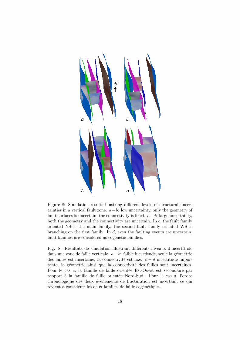
Figure 8: Simulation results illustring different levels of structural uncer-tainties in a vertical fault zone. a− b: low uncertainty, only the geometry offault surfaces is uncertain, the connectivity is fixed. c−d: large uncertainty,both the geometry and the connectivity are uncertain. In c, the fault familyoriented NS is the main family, the second fault family oriented WS isbranching on the first family. In d, even the faulting events are uncertain,fault families are considered as cogenetic families.

Fig. 8. Resultats de simulation illustrant differents niveaux d’incertitudedans une zone de faille verticale. a− b: faible incertitude, seule la geometriedes failles est incertaine, la connectivite est fixe. c − d incertitude impor-tante, la geometrie ainsi que la connectivite des failles sont incertaines.Pour le cas c, la famille de faille orientee Est-Ouest est secondaire parrapport a la famille de faille orientee Nord-Sud. Pour le cas d, l’ordrechronologique des deux evenements de fracturation est incertain, ce quirevient a considerer les deux familles de faille cogenetiques.

18