Stochastic Simulation and Applications in Finance with MATLAB® Programs (Huynh/Stochastic) ||...

4

Introduction to Computer Simulationof Random Variables

In finance, as in many other areas of social and human sciences, it is often very difficult or evenimpossible to find an analytical solution for most of the problems we have to solve. This is thecase with the evaluation of complex and interdependent financial products. However, there aremany numerical techniques available to evaluate these products. One of the techniques thatwe present in this book is the computer based simulation method. From its inherent nature,this method offers a wide flexibility, especially when evaluating financial products dependenton many state variables.

How can a computer generate random events, since if it executes a given algorithm knowingthe initial result, we should be able to guess the results at the outset? In fact, results generatedon a computer are not conceptually random but, from the point of view of an observer, behavelike random ones.

These results occur with a statistical regularity as discussed in the previous chapters. Theregularity associated with the results generated by a computer can be explained as follows: ifthe algorithm generated by a computer is chaotic then it will produce unpredictable results foran observer. Thus, to build a dynamically chaotic algorithm is sufficient to generate randomevents.

The previous chapters showed how to obtain random variables for which we know thedistribution function from a uniform random variable. The problem of generating randomvariables on computer is the same as generating a uniform random variable.

In order to generate a uniform random variable without resorting to a complex chaoticdynamic, all we need to do is to build an algorithm such that the generated result has thestatistical regularity of a uniform random variable.

If the generated number is expressed with a binary representation, the number of 0 and 1should be approximately equal, the number of two following 0 and two following 1 should beapproximately equal, etc.

In the last 50 years, we have seen researchers focussing on building algorithms that yield thisstatistical regularity. Because a computer has a finite precision, the generator can’t generatean infinite number of different outcomes but only a finite number of results. This means thatthe series of generated results is periodic. Generally, we choose the algorithm that gives us thelongest possible period.

In this chapter, we define basic concepts regarding the generation of random variables oncomputers and we present the techniques used to generate some widely used random variablesin finance. After that, we present the simulation of random vectors using variance-covariancematrix decomposition techniques such as the Cholesky decomposition and the eigenvaluedecomposition. The financial assets variance-covariance matrix decomposition is important inthe study of risk factors, and more precisely in the pricing of financial instruments and riskmanagement. Finally, we introduce the acceptance-rejection and Monte Carlo Markov Chain(MCMC) generation methods that could both be used in many simulation cases in finance.

Stochastic Simulation and Applications in Finance with MATLAB® Programsby Huu Tue Huynh, Van Son Lai and Issouf Soumaré

Copyright © 2008, John Wiley & Sons Ltd.

48 Stochastic Simulation and Applications in Finance

In this chapter, as well as in the followings, we include MATLAB R© programs in order toillustrate the theory presented. A list of most frequently used functions in MATLAB is givenin Appendix B.

4.1 UNIFORM RANDOM VARIABLE GENERATOR

As discussed above, the series of numbers generated by the computer must have the longestpossible period. The most frequently used algorithm is of the form:

xn+1 = axn + b ( mod m). (4.1)

The series of results obtained from an initial value corresponds to the realization of a sequenceof uniform random variables on the set

{0, 1, 2, . . . , m − 1}. (4.2)

In reality, in order for the period of the series generated with this algorithm to be m, wemust choose integer a, b and m in an appropriate way, because this period is equal to m if andonly if

(i) b is relatively prime with m,(ii) a − 1 is a multiple of any prime number that divides m, for example a multiple of 3 if m

is a multiple of 3.

The parameters used by MATLAB’s generator are described in Moler (1995) and given by:

m = 231 − 1 = 2147483647,

b = 0, and

a = 75 = 16807.

This algorithm generates a series of integer numbers between 0 and m − 1. If we divide theresult by m, we get results in the interval [0, 1]. Since m is very large, the difference between2 successive numbers is relatively small and thus we can consider this discrete variable to bea continuous variable in [0, 1].

In MATLAB, to generate a uniform random variable between 0 and 1, often denoted byU(0, 1), we use the command rand. The command rand generates one random variableuniformly distributed on the interval [0, 1]. The command rand (m, n) generates m × nrandom variables uniformly distributed on [0, 1] and stocked in a matrix of m rows and ncolumns.

From the examples presented in previous chapters, a uniformly distributed random variableon the set [a, b] called U(a, b) can be generated from the variable U(0, 1) using the relation

U (a, b) = (b − a)U (0, 1) + a. (4.3)

4.2 GENERATING DISCRETE RANDOM VARIABLES

4.2.1 Finite Discrete Random Variables

Let the random variable X on the finite space of events {x1, x2, . . . , xn} have the respectiveprobabilities p1, p2, . . . , pn. We can simulate X with a uniform random variable U(0, 1) in

Introduction to Computer Simulation of Random Variables 49

setting:

X = x1 if U ≤ p1, (4.4)

X = x2 if p1 < U ≤ p1 + p2, (4.5)...

X = xn if p1 + p2 + · · · + pn−1 < U ≤ p1 + p2 + · · · + pn. (4.6)

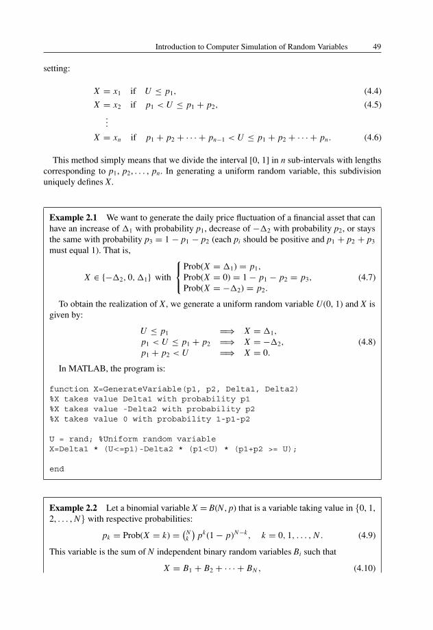
This method simply means that we divide the interval [0, 1] in n sub-intervals with lengthscorresponding to p1, p2, . . . , pn. In generating a uniform random variable, this subdivisionuniquely defines X.

Example 2.1 We want to generate the daily price fluctuation of a financial asset that canhave an increase of �1 with probability p1, decrease of −�2 with probability p2, or staysthe same with probability p3 = 1 − p1 − p2 (each pi should be positive and p1 + p2 + p3

must equal 1). That is,

X ∈ {−�2, 0,�1} with

⎧⎨⎩Prob(X = �1) = p1,

Prob(X = 0) = 1 − p1 − p2 = p3,

Prob(X = −�2) = p2.

(4.7)

To obtain the realization of X, we generate a uniform random variable U(0, 1) and X isgiven by:

U ≤ p1 =⇒ X = �1,

p1 < U ≤ p1 + p2 =⇒ X = −�2,

p1 + p2 < U =⇒ X = 0.

(4.8)

In MATLAB, the program is:

function X=GenerateVariable(p1, p2, Delta1, Delta2)%X takes value Delta1 with probability p1%X takes value -Delta2 with probability p2%X takes value 0 with probability 1-p1-p2

U = rand; %Uniform random variableX=Delta1 * (U<=p1)-Delta2 * (p1<U) * (p1+p2 >= U);

end

Example 2.2 Let a binomial variable X = B(N, p) that is a variable taking value in {0, 1,2, . . . , N} with respective probabilities:

pk = Prob(X = k) = (Nk

)pk(1 − p)N−k, k = 0, 1, . . . , N . (4.9)

This variable is the sum of N independent binary random variables Bi such that

X = B1 + B2 + · · · + BN , (4.10)


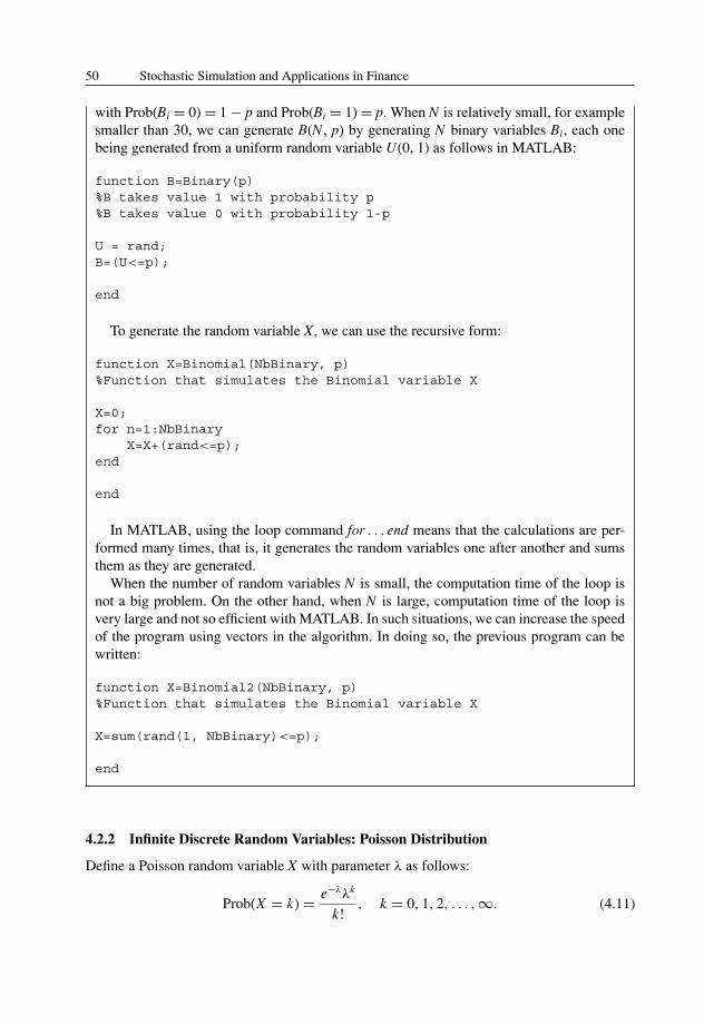
with Prob(Bi = 0) = 1 − p and Prob(Bi = 1) = p. When N is relatively small, for examplesmaller than 30, we can generate B(N, p) by generating N binary variables Bi, each onebeing generated from a uniform random variable U(0, 1) as follows in MATLAB:

function B=Binary(p)%B takes value 1 with probability p%B takes value 0 with probability 1-p

U = rand;B=(U<=p);

end

To generate the random variable X, we can use the recursive form:

function X=Binomial(NbBinary, p)%Function that simulates the Binomial variable X

X=0;for n=1:NbBinary

X=X+(rand<=p);end

end

In MATLAB, using the loop command for . . . end means that the calculations are per-formed many times, that is, it generates the random variables one after another and sumsthem as they are generated.

When the number of random variables N is small, the computation time of the loop isnot a big problem. On the other hand, when N is large, computation time of the loop isvery large and not so efficient with MATLAB. In such situations, we can increase the speedof the program using vectors in the algorithm. In doing so, the previous program can bewritten:

function X=Binomial2(NbBinary, p)%Function that simulates the Binomial variable X

X=sum(rand(1, NbBinary)<=p);

end

4.2.2 Infinite Discrete Random Variables: Poisson Distribution

Define a Poisson random variable X with parameter λ as follows:

Prob(X = k) = e−λλk

k!, k = 0, 1, 2, . . . ,∞. (4.11)


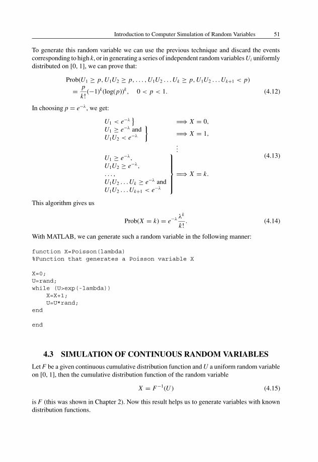
To generate this random variable we can use the previous technique and discard the eventscorresponding to high k, or in generating a series of independent random variables Ui uniformlydistributed on [0, 1], we can prove that:

Prob(U1 ≥ p, U1U2 ≥ p, . . . , U1U2 . . . Uk ≥ p, U1U2 . . . Uk+1 < p)

= p

k!(−1)k(log(p))k, 0 < p < 1. (4.12)

In choosing p = e−λ, we get:

U1 < e−λ} =⇒ X = 0,

U1 ≥ e−λ andU1U2 < e−λ

}=⇒ X = 1,

...U1 ≥ e−λ,

U1U2 ≥ e−λ,

. . . ,

U1U2 . . . Uk ≥ e−λ andU1U2 . . . Uk+1 < e−λ

⎫⎪⎪⎪⎪⎬⎪⎪⎪⎪⎭ =⇒ X = k.

(4.13)

This algorithm gives us

Prob(X = k) = e−λ λk

k!. (4.14)

With MATLAB, we can generate such a random variable in the following manner:

function X=Poisson(lambda)%Function that generates a Poisson variable X

X=0;U=rand;while (U>exp(-lambda))

X=X+1;U=U*rand;

end

end

4.3 SIMULATION OF CONTINUOUS RANDOM VARIABLES

Let F be a given continuous cumulative distribution function and U a uniform random variableon [0, 1], then the cumulative distribution function of the random variable

X = F−1(U ) (4.15)

is F (this was shown in Chapter 2). Now this result helps us to generate variables with knowndistribution functions.


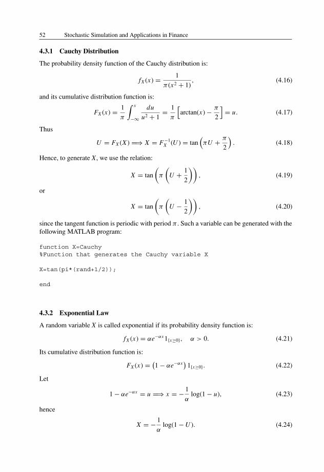
4.3.1 Cauchy Distribution

The probability density function of the Cauchy distribution is:

fX (x) = 1

π (x2 + 1), (4.16)

and its cumulative distribution function is:

FX (x) = 1

π

∫ x

−∞

du

u2 + 1= 1

π

[arctan(x) − π

2

]= u. (4.17)

Thus

U = FX (X ) =⇒ X = F−1X (U ) = tan

(πU + π

2

). (4.18)

Hence, to generate X, we use the relation:

X = tan

(π

(U + 1

2

)), (4.19)

or

X = tan

(π

(U − 1

2

)), (4.20)

since the tangent function is periodic with period π . Such a variable can be generated with thefollowing MATLAB program:

function X=Cauchy%Function that generates the Cauchy variable X

X=tan(pi*(rand+1/2));

end

4.3.2 Exponential Law

A random variable X is called exponential if its probability density function is:

fX (x) = αe−αx 1{x≥0}, α > 0. (4.21)

Its cumulative distribution function is:

FX (x) = (1 − αe−αx

)1{x≥0}. (4.22)

Let

1 − αe−αx = u =⇒ x = − 1

αlog(1 − u), (4.23)

hence

X = − 1

αlog(1 − U ). (4.24)


Since U is uniformly distributed on [0, 1], then 1 − U is also uniformly distributed on [0, 1].It follows that X can be generated by:

X = − 1

αlog(U ), (4.25)

where U is a uniform random variable on [0, 1]. In MATLAB, this procedure gives:

function X=Exp(alpha)%Function that generates the Exponential variable X

X = -log(rand)/alpha;

end

4.3.3 Rayleigh Random Variable

X is a Rayleigh random variable if its density function is equal to

fX (x) = xe− x2

2 1{x≥0}. (4.26)

Its cumulative distribution function is then:

FX (x) =∫ x

0ve− v2

2 dv = 1 − e− x2

2 = u =⇒ x =√

−2 log(1 − u). (4.27)

X can therefore be generated from a uniform random variable U(0, 1) by the relation:

X =√

−2 log(1 − U ). (4.28)

Since 1 − U also follows a uniform law on [0, 1], we can directly generate X by:

X =√

−2 log(U ). (4.29)

The MATLAB program is

function X=Rayleigh%Function that generates the Rayleigh variable X

X = sqrt(-2*log(rand));

end

4.3.4 Gaussian Distribution

Consider a standard Gaussian random variable X with zero mean and unit variance, denotedby N(0, 1). X can be generated following three different approaches.

Method 1

Let 12 random variables {Ui}i=1, . . . ,12 uniformly distributed on [0, 1], we study their sum:

X = U1 + U2 + . . . + U12 − 6. (4.30)


Since

E [Ui ] = 1

2and Var [Ui ] = 1

12, (4.31)

it follows:

E [X ] = 0 and Var [X ] = 1. (4.32)

X is thus of zero mean and unit variance. Since X is the sum of 12 independent random variableshaving the same probability law, by virtue of the central limit theorem, we can consider X asa Gaussian variable. This way of generating a Gaussian random variable is interesting but notvery precise since it is not possible to obtain rare events at the tail of the distribution. In fact,with this simulation Prob(X > 6) = 0 but for a standard Gaussian random variable Prob(X >

6) � 10−7.The program in MATLAB is:

function X=Gaussian1%Generation of a Gaussian variable with method 1

X = sum(rand(1,12))-6;

end

Method 2

We saw in Chapter 2 that two Gaussian random variables X and Y with mean of 0 and varianceof 1 can be generated from a Rayleigh variable with density

fρ(ρ) = ρe− ρ2

2 1{ρ≥0} (4.33)

and a uniform random variable on [0, 2π ] of density

fθ (θ ) = 1

2π, 0 ≤ θ ≤ 2π. (4.34)

For the simulation, we set

X = ρ cos(θ ) (4.35)

and

Y = ρ sin(θ ). (4.36)

We saw that ρ and θ can be generated from two uniformly distributed random variables on[0, 1]:

ρ =√

−2 log(U1) (4.37)

and

θ = 2πU2. (4.38)


Then we can generate two Gaussian random variables from two uniform random variables on[0, 1] with the following formulas known as the Box-Muller method:

X =√

−2 log(U1) cos(2πU2) (4.39)

and

Y =√

−2 log(U1) sin(2πU2). (4.40)

The program in MATLAB language is:

function [X,Y]=Gaussian2%Function that generates two Gaussian random variables with method 2

U1=rand;U2=rand;X=sqrt(-2*log(U1))*cos(2*pi*U2);Y=sqrt(-2*log(U1))*sin(2*pi*U2);

end

Method 3

In MATLAB, the command randn directly generates a Gaussian random variable with meanof 0 and variance of 1. If we want to generate a matrix n × m with elements being Gaussianwith zero mean and unit variance, the command is randn(n, m).

Thus, in MATLAB, in order to generate a Gaussian random variable X with mean μ andvariance σ 2, the command is:

function X=Gaussian3(mu,sigma)%Function that generates a Gaussian variable X%with mean mu and standard deviation sigma with method 3

X = sigma * randn + mu;

end

We now compare all three methods of generating Gaussian random variables. We present asmall program generating N Gaussian random variables following each of the three methods.We also compute their means and standard deviations.

function Gaussian(N)%Function that compares the different methods of generating% a Gaussian random variable%N must be an even number

%Method 1A = sum(rand(N,12),2) - 6;MeanA = mean(A,1);


Table 4.1 Mean and standard deviation using the three methods for generating aGaussian random variable

Method 1 Method 2 Method 3

N Mean Std. Mean Std. Mean Std.

10 0.1066 1.4399 0.0007 1.0938 0.3265 0.1817102 −0.1719 0.9127 −0.1286 0.9488 0.0188 1.0673103 0.0517 0.9755 −0.0296 0.9886 0.0253 0.9677104 0.0044 1.0155 −0.0023 1.0194 −0.0035 0.9967105 −0.0062 1.0009 −0.0048 1.0024 0.0015 1.0044106 0.0019 0.9991 −0.0015 1.0005 0.0002 1.0009

StdA = std(A);sprintf(’Method 1 \n Mean: %g, Standard deviation: %g’, MeanA, StdA)

%Method 2U1 = rand(1,N/2);U2 = rand(1,N/2);B1 = sqrt(-2*log(U1)).*cos(2*pi*U2);B2 = sqrt(-2*log(U1)).*sin(2*pi*U2);B = [B1,B2]’;MeanB = mean(B);StdB = std(B);sprintf(’Method 2 \n Mean: %g, Standard deviation: %g’, MeanB, StdB)

%Method 3C = randn(N,1);MeanC = mean(C);StdC = std(C);sprintf(’Method 3 \n Mean: %g, Standard deviation: %g’, MeanC, StdC)end

We call the program with different values for N. Table 4.1 simply shows the simulated meanand standard deviation of a standardized normal random variable (mean zero and standarddeviation one) using each of the three methods.

4.4 SIMULATION OF RANDOM VECTORS

In this section, we would like to generate a Gaussian random vector X having a knownvariance-covariance matrix �X = cov(X , X�). Let Z = (Z1, . . . , Zn)� be an independentGaussian random vector of zero mean and unit variance: Z ∼ N (0, I ), that is

E[Z ] = 0 and Var(Z ) = I, (4.41)

where I is the identity matrix with 1 on the diagonal and 0 elsewhere. We want to use such avector to create the random vector X . We include a review on matrix algebra in Appendix A.


4.4.1 Case of a Two-Dimensional Random Vector

We want to generate the vector X with the following properties:

X =(

X1

X2

)∼ N

(0,

(σ 2

1 ρσ1σ2

ρσ1σ2 σ 22

)). (4.42)

Then

E[Xi ] = 0, E[X2i ] = σ 2

i , E[X1 X2] = ρσ1σ2. (4.43)

Let the Gaussian random vector

Z =(

Z1

Z2

)∼ N

(0,

(1 00 1

)). (4.44)

Then setting

X1 = σ1 Z1

X2 = αZ1 + βZ2, (4.45)

we obtain

E[X1 X2] = ασ1 E[Z21] = ασ1. (4.46)

However, we want to have E[X1X2] = ρσ 1σ 2, hence α = ρσ 2. Moreover

Var(X2) = α2 + β2 = σ 22 ⇒ β = ±

√σ 2

2 (1 − ρ2). (4.47)

We choose β =√

σ 22 (1 − ρ2). Hence(

X1

X2

)=(

σ1 0ρσ2

√1 − ρ2σ2

)(Z1

Z2

). (4.48)

Thus, we can generate such variables in MATLAB using the following program:

function rep=RandomVector(sigma1, sigma2, rho)%Generation of a random vector of dimension 2 and correlation rho

MatrixL = [sigma1, 0;rho*sigma2, sigma2*sqrt(1-rhoˆ2)];rep = MatriceL*randn(2, 1);

end

4.4.2 Cholesky Decomposition of the Variance-Covariance Matrix

In the more general case of any n-dimensional random vector, if we take

X = L Z =⇒ cov(X , X�) = E[L Z Z�L�], (4.49)


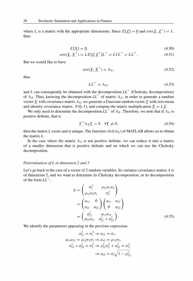
where L is a matrix with the appropriate dimensions. Since E[Z ] = 0 and cov(Z , Z�) = I,then

E[X ] = 0, (4.50)

cov(X , X�) = L E[Z Z�]L� = L I L� = L L�. (4.51)

But we would like to have

cov(X , X�) = �X , (4.52)

thus

L L� = �X , (4.53)

and L can consequently be obtained with the decomposition LL� (Cholesky decomposition)of �X . Thus, knowing the decomposition LL� of matrix �X , in order to generate a randomvector X with covariance matrix �X , we generate a Gaussian random vector Z with zero meanand identity covariance matrix, N (0, I ), and compute the matrix multiplication X = L Z .

We only need to determine the decomposition LL� of �X . Therefore, we note that if �X ispositive definite, that is

Y ��X Y > 0 ∀Y = 0, (4.54)

then the matrix L exists and is unique. The function chol(�X) of MATLAB allows us to obtainthe matrix L.

In the case where the matrix �X is not positive definite, we can reduce it into a matrixof a smaller dimension that is positive definite and on which we can use the Choleskydecomposition.

Determination of L in dimension 2 and 3

Let’s go back to the case of a vector of 2 random variables. Its variance-covariance matrix A isof dimension 2, and we want to determine its Cholesky decomposition, or its decompositionof the form LL�:

A =(

σ 21 ρ12σ1σ2

ρ12σ2σ1 σ 22

)

=(

a11 0

a21 a22

)(a11 a12

0 a22

)

=(

a211 a11a12

a21a11 a221 + a2

22

). (4.55)

We identify the parameters appearing in the previous expression.

a211 = σ 2

1 ⇒ a11 = σ1,

a11a12 = ρ12σ1σ2 ⇒ a12 = ρ12σ2,

a212 + a2

22 = σ 22 ⇒ ρ2

12σ22 + a2

22 = σ 22 ,

⇒ a22 = σ2

√1 − ρ2

12,


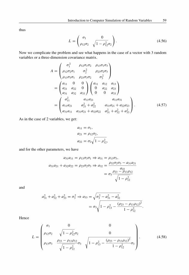
thus

L =(

σ1 0

ρ12σ2

√1 − ρ2

12σ2

). (4.56)

Now we complicate the problem and see what happens in the case of a vector with 3 randomvariables or a three-dimension covariance matrix.

A =

⎛⎜⎝ σ 21 ρ12σ1σ2 ρ13σ1σ3

ρ12σ2σ1 σ 22 ρ23σ2σ3

ρ13σ3σ1 ρ23σ3σ2 σ 23

⎞⎟⎠=⎛⎝a11 0 0

a21 a22 0a31 a32 a33

⎞⎠⎛⎝a11 a12 a13

0 a22 a23

0 0 a33

⎞⎠=

⎛⎜⎝ a211 a11a21 a11a31

a11a21 a221 + a2

22 a31a21 + a22a23

a31a11 a31a21 + a32a22 a231 + a2

32 + a233

⎞⎟⎠ . (4.57)

As in the case of 2 variables, we get:

a11 = σ1,

a21 = ρ12σ2,

a22 = σ2

√1 − ρ2

12,

and for the other parameters, we have

a31a11 = ρ13σ3σ1 ⇒ a31 = ρ13σ3,

a31a21 + a32a22 = ρ23σ2σ3 ⇒ a32 = ρ32σ2σ3 − a31a21

a22

= σ3ρ23 − ρ13ρ12√

1 − ρ212

and

a231 + a2

32 + a233 = σ 2

3 ⇒ a33 =√

σ 23 − a2

31 − a232

= σ3

√1 − ρ2

13 − (ρ23 − ρ13ρ12)2

1 − ρ212

.

Hence

L =

⎛⎜⎜⎜⎜⎜⎝σ1 0 0

ρ12σ2

√1 − ρ2

12σ2 0

ρ13σ3ρ23 − ρ13ρ12√

1 − ρ212

σ3

√1 − ρ2

13 − (ρ23 − ρ13ρ12)2

1 − ρ212

σ3

⎞⎟⎟⎟⎟⎟⎠ . (4.58)


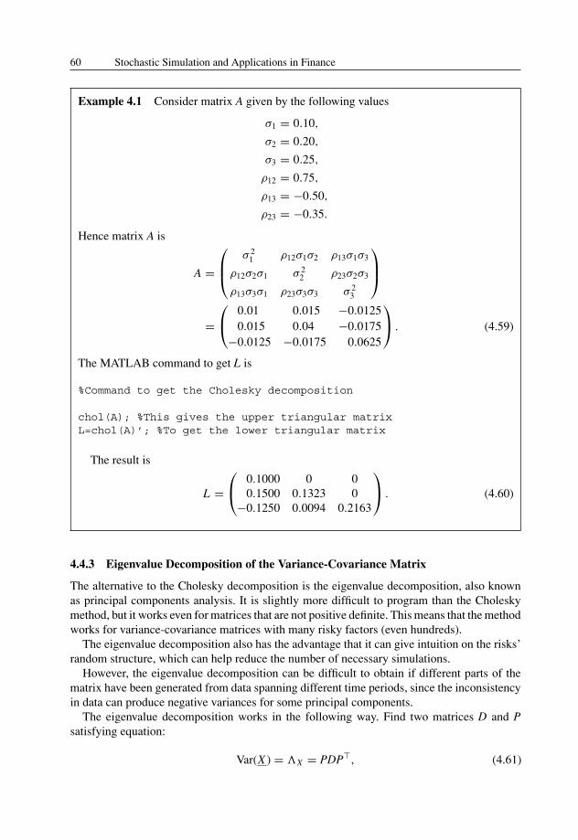
Example 4.1 Consider matrix A given by the following values

σ1 = 0.10,

σ2 = 0.20,

σ3 = 0.25,

ρ12 = 0.75,

ρ13 = −0.50,

ρ23 = −0.35.

Hence matrix A is

A =

⎛⎜⎝ σ 21 ρ12σ1σ2 ρ13σ1σ3

ρ12σ2σ1 σ 22 ρ23σ2σ3

ρ13σ3σ1 ρ23σ3σ3 σ 23

⎞⎟⎠=⎛⎝ 0.01 0.015 −0.0125

0.015 0.04 −0.0175−0.0125 −0.0175 0.0625

⎞⎠ . (4.59)

The MATLAB command to get L is

%Command to get the Cholesky decomposition

chol(A); %This gives the upper triangular matrixL=chol(A)’; %To get the lower triangular matrix

The result is

L =⎛⎝ 0.1000 0 0

0.1500 0.1323 0−0.1250 0.0094 0.2163

⎞⎠ . (4.60)

4.4.3 Eigenvalue Decomposition of the Variance-Covariance Matrix

The alternative to the Cholesky decomposition is the eigenvalue decomposition, also knownas principal components analysis. It is slightly more difficult to program than the Choleskymethod, but it works even for matrices that are not positive definite. This means that the methodworks for variance-covariance matrices with many risky factors (even hundreds).

The eigenvalue decomposition also has the advantage that it can give intuition on the risks’random structure, which can help reduce the number of necessary simulations.

However, the eigenvalue decomposition can be difficult to obtain if different parts of thematrix have been generated from data spanning different time periods, since the inconsistencyin data can produce negative variances for some principal components.

The eigenvalue decomposition works in the following way. Find two matrices D and Psatisfying equation:

Var(X ) = �X = PDP�, (4.61)


where �X is the variance-covariance matrix, D is a matrix such that the only non zero elementsare the ones on the diagonal, and P is an orthogonal matrix, that is:

I = PP�. (4.62)

This method rests on the eigenvectors forming a basis, which is guaranteed in this case sincethe matrix �X is symmetric. The elements on the diagonal of matrix D are the eigenvalues ofmatrix �X . Knowing that D is a diagonal matrix with all positive elements

D =

⎛⎜⎝ d1 0 0

0. . . 0

0 0 dn

⎞⎟⎠ , (4.63)

the matrix �X can be partitioned in two, such that

�X = L L�, with L = P√

D, (4.64)

and

√D =

⎛⎜⎝√

d1 0 0

0. . . 0

0 0√

dn

⎞⎟⎠ . (4.65)

From this decomposition of matrix �X , the vector X can be obtained exactly as in the case ofthe Cholesky decomposition in setting

X = L Z , (4.66)

with the vector Z being composed of n independent random variables with unit variance, thatis, Var(Z ) = I .

Example 4.2 If we take the matrix A given previously, that is

A =⎛⎝ 0.01 0.015 −0.0125

0.015 0.04 −0.0175−0.0125 −0.0175 0.0625

⎞⎠ . (4.67)

We obtain the following matrices P and D

P =⎛⎝ 0.9367 0.2285 −0.2652

−0.3359 0.7998 −0.49750.0985 0.5551 0.8259

⎞⎠ (4.68)

D =⎛⎝ 0.0033 0 0

0 0.0321 00 0 0.0771

⎞⎠ . (4.69)

These matrices can be computed in MATLAB with the command

%Command giving the eigenvalues and eigenvectors%of matrix A

[P,D] = eig(A); %P->eigenvectors’ matrix%D->corresponding eigenvalues’ matrix


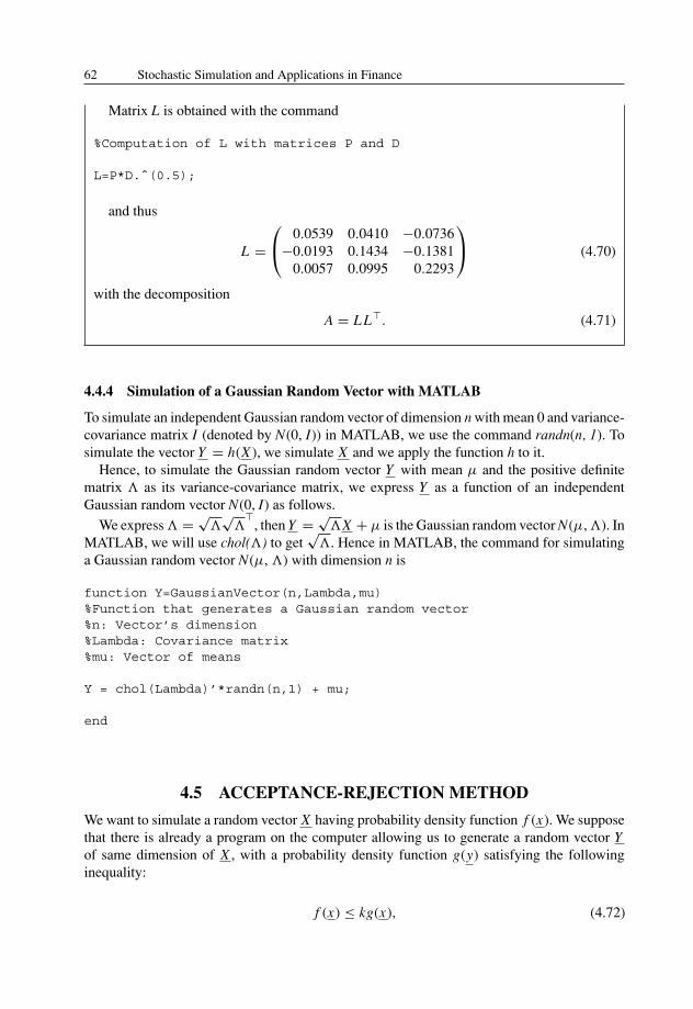
Matrix L is obtained with the command

%Computation of L with matrices P and D

L=P*D.ˆ(0.5);

and thus

L =⎛⎝ 0.0539 0.0410 −0.0736

−0.0193 0.1434 −0.13810.0057 0.0995 0.2293

⎞⎠ (4.70)

with the decomposition

A = L L�. (4.71)

4.4.4 Simulation of a Gaussian Random Vector with MATLAB

To simulate an independent Gaussian random vector of dimension n with mean 0 and variance-covariance matrix I (denoted by N(0, I)) in MATLAB, we use the command randn(n, 1). Tosimulate the vector Y = h(X ), we simulate X and we apply the function h to it.

Hence, to simulate the Gaussian random vector Y with mean μ and the positive definitematrix � as its variance-covariance matrix, we express Y as a function of an independentGaussian random vector N(0, I) as follows.

We express � = √�

√�

�, then Y = √

�X + μ is the Gaussian random vector N(μ, �). InMATLAB, we will use chol(�) to get

√�. Hence in MATLAB, the command for simulating

a Gaussian random vector N(μ, �) with dimension n is

function Y=GaussianVector(n,Lambda,mu)%Function that generates a Gaussian random vector%n: Vector’s dimension%Lambda: Covariance matrix%mu: Vector of means

Y = chol(Lambda)’*randn(n,1) + mu;

end

4.5 ACCEPTANCE-REJECTION METHOD

We want to simulate a random vector X having probability density function f (x). We supposethat there is already a program on the computer allowing us to generate a random vector Yof same dimension of X , with a probability density function g(y) satisfying the followinginequality:

f (x) ≤ kg(x), (4.72)


where k is a given positive constant. We set

α(x) = f (x)

kg(x). (4.73)

Generation algorithm1- We generate the vector Y 1 with probability density function g(y) and a random variable U1

independent of Y 1, uniformly distributed between 0 and 1.2- If U1 ≤ α(Y 1), we choose X = Y 1, otherwise we reject Y 1 and re-generate new Y and Uuntil Um ≤ α(Y m), then we will choose X = Y m . This way, the generated random vector Xfollows the probability law f (x).

In order to illustrate this result, we consider the event {X ∈ E}, where E is a subset of thereal axis. Because Y m and Um are all independent, we immediately note that the events

{X = Y 1}, {X = Y 2}, . . . , {X = Y m} (4.74)

are mutually exclusive, which gives

Prob(X ∈ E) = Prob({X = Y 1, X ∈ E} or . . .

or {X = Y m, X ∈ E} or . . .)

=∞∑

m=1

Prob({X = Y m, X ∈ E}). (4.75)

We know that

Prob({X = Y m, X ∈ E}) = Prob({U1 > α(Y 1)} ∩ {U2 > α(Y 2)} ∩ . . .

∩ {Um−1 > α(Y m−1)} ∩ {Um ≤ α(Y m)}∩ {Y m ∈ E})

= Prob({U1 > α(Y 1)}) ×Prob({U2 > α(Y 2)}) × . . .

× Prob({Um−1 > α(Y m−1)})× Prob({Um ≤ α(Y m), Y m ∈ E})

= (1 − p)m−1Prob(Y m ∈ E | Um ≤ α(Y m))

× Prob(Um ≤ α(Y m)), (4.76)

where p = Prob(U ≤ α(Y )).Since

Prob(Y m ∈ E | Um ≤ α(Y m)) (4.77)

is identical to

Prob(Y ∈ E | U ≤ α(Y )), (4.78)

we have

Prob({X = Y m, X ∈ E}) = p(1 − p)m−1Prob(Y ∈ E | U ≤ α(Y )). (4.79)


Finally,

Prob(X ∈ E) =∞∑

m=1

p(1 − p)m−1Prob(Y ∈ E | U ≤ α(Y ))

= pProb(Y ∈ E | U ≤ α(Y ))∞∑

m=1

(1 − p)m−1

= Prob(Y ∈ E | U ≤ α(Y ))

= Prob(Y ∈ E, U ≤ α(Y ))

Prob(U ≤ α(Y )). (4.80)

To determine Prob(X ∈ E), we must compute Prob(Y ∈ E, U ≤ α(Y )) and Prob(U ≤ α(Y )).We have

Prob(U ≤ α(Y )) =∫

Prob(U ≤ α(y))g(y)dy

=∫

α(Y )g(y)dy

=∫ f (y)

kg(y)g(y)dy

= 1

k, (4.81)

and

Prob(Y ∈ E, U ≤ α(Y )) =∫

Eg(y)dy

∫ α(y)

0du

=∫

Eα(y)g(y)dy

=∫

E

f (y)

kg(y)g(y)dy

= 1

k

∫E

f (y)dy. (4.82)

Which gives

Prob(X ∈ E) =∫

Ef (x)dx . (4.83)

This relation shows that the probability density function of X is effectively f (x).

Remark 5.1 We have shown that Prob(U ≤ α(Y )) = 1k , which means that the rate of rejection

is very high when k is large. When k approaches 1, the rate of rejection decreases rapidly.Thus, in practice, we should choose a function g(y) with values of similar size to f (x).


4.6 MARKOV CHAIN MONTE CARLO METHOD (MCMC)

4.6.1 Definition of a Markov Process

Let a random process {Xn, n = 0, 1, 2, . . . } be given. Refer to Chapter 7 for a more detailedanalysis of random processes.

We suppose that Xn take their values in the states’ set Ω. We say that the process {Xn, n =0, 1, 2, . . . } is a Markov chain if

Prob(Xn+1 = xn+1 | Xn = xn, Xn−1 = xn−1, . . . , X0 = x0) (4.84)

is equal to

Prob(Xn+1 = xn+1 | Xn = xn). (4.85)

It means that the probability that the process is in state xn+1 at n + 1, knowing that is wasin state xn at n, is independent of everything that happened before n. All that matters are thesuccessive moments n and n + 1.

Moreover, the Markov chain will be called homogeneous if

Prob(Xn+1 = y | Xn = x) = px,y . (4.86)

That is, the probability of being in state y knowing that the process was in state x previously,px,y, is totally independent of n. All that matters is the evolution between two successive dates.

4.6.2 Description of the MCMC Technique

We will show in Chapter 5 that the so-called Monte Carlo method can be used to estimatethe mathematical expectation of a random quantity q(X), where X is a random variable withprobability density function fX(x):

E[q(X )] ≈ 1

N

N∑n=1

q(Xn), (4.87)

where the samples Xn are independently generated by computer.It is not always easy to directly generate Xn if fX(x) is complicated. Because the estimator

(6.4) doesn’t require the independence hypothesis for the Xn, we can use any method togenerate them, provided that Xn has fX(x) as its density function. This explains the idea ofusing a Markov chain.

Suppose that we have a homogeneous Markov chain such that the successive states {X0,X1, X2, . . . } are characterized by the transition probability

Prob(Xn+1 | Xn). (4.88)

The homogeneity ensures that Prob(Xn+1 | Xn) doesn’t depend on n.How does the choice of X0 affect Xn? Expressed differently, what is the form of fXn (x |x0)?

It is known that, under very general regularity conditions, fXn (x |x0) becomes independent ofx0 when n is very large, that is, when the chain is in a stationary regime.

We denote by ϕX(x) the density function of X in the state when the chain reaches thepermanent regime assuming that we can construct the chain such that ϕX(x) is identical to thedesired fX(x). We let the chain evolve until it reaches the stationary regime (i.e., large M) and


then use the following simulated states to estimate E[q(X)]:

E[q(X )] ≈ 1

N − M

N∑n=M+1

q(Xn). (4.89)

This result of using part of the simulated states to estimate the expected value is known underthe name “ergodic mean”.

The most widely known method of generating a Markov chain with ϕX(x) identical to fX(x)is the Metropolis-Hastings algorithm. Let g(x |y) be any conditional density function.

Let’s define

α(x, y) = min(1,

fX (y)g(x |y)

fX (x)g(y|x)

). (4.90)

Assuming that at any time n, the chain is in state Xn = xn, in order to construct the desiredMarkov chain we generate two random variables. The first, Y , is characterized by the densityfunction g(y|xn) and the second one, Un, is independent of the first and is uniformly distributedbetween 0 and 1. Xn+1 is then defined by

Xn+1 ={Y, if U ≤ α(xn, y);

Xn, if U > α(xn, y).(4.91)

As seen in Section 4.5, this is precisely the rejection method.It is important to note that since there is no predefined form for g(y|x), we will choose a

particular formulation in order to suit the model under study.

Notes and Complementary Readings

For further readings, readers can eventually refer to the following publications on Monte Carlosimulations and numerical methods: Kloeden, Platen and Schurz (1997), Press, Teukolsky,Vetterling and Flannery (1992), Rubinstein (1981) and Seydel (2002).

For a quick learning of MATLAB, the reader can refer to Etter and Kuncicky (2002)and Pratap (2002), and for complementary references on random variables generation withMATLAB, we suggest Martinez and Martinez (2002).

Useful references on Markov chains and random processes are the books of Ross (2002 aand b) and Kloeden and Platen (1992).

Stochastic Simulation and Applications in Finance with MATLAB® Programs (Huynh/Stochastic) ||...

Documents

Transcript of Stochastic Simulation and Applications in Finance with MATLAB® Programs (Huynh/Stochastic) ||...