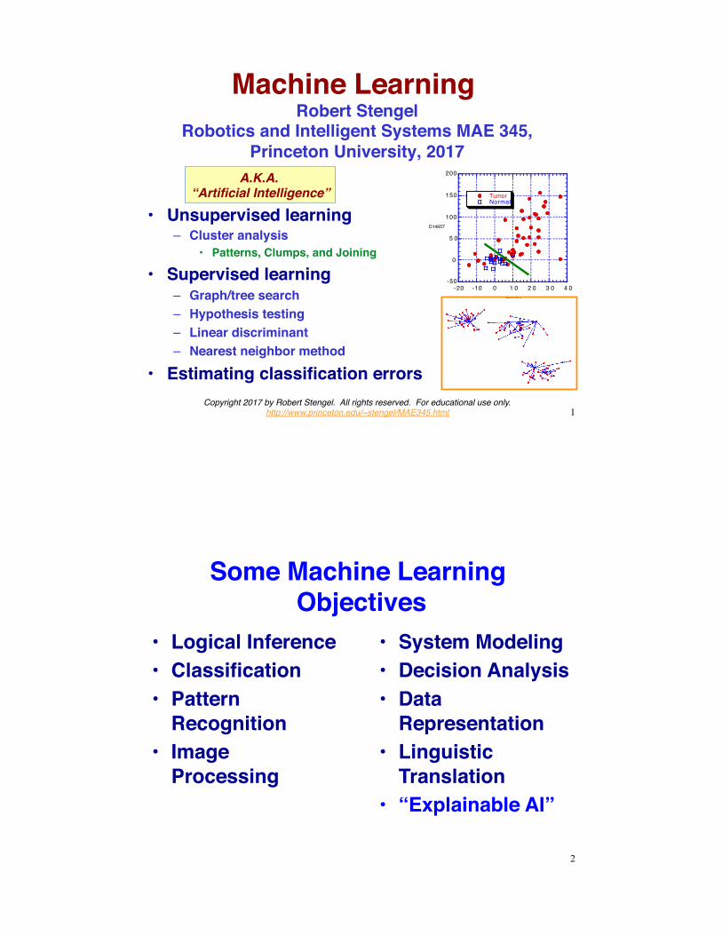
Machine Learning !Robert Stengel!

Robotics and Intelligent Systems MAE 345, !Princeton University, 2017

•! Unsupervised learning–! Cluster analysis

•! Patterns, Clumps, and Joining

•! Supervised learning–! Graph/tree search–! Hypothesis testing–! Linear discriminant–! Nearest neighbor method

•! Estimating classification errors

-50

0

5 0

100

150

200

-20 -10 0 1 0 2 0 3 0 4 0

TumorNormal

D14657

M94363

Copyright 2017 by Robert Stengel. All rights reserved. For educational use only.http://www.princeton.edu/~stengel/MAE345.html

A.K.A. “Artificial Intelligence”

1

Some Machine Learning Objectives

2

•! Logical Inference•! Classification•! Pattern

Recognition•! Image

Processing

•! System Modeling•! Decision Analysis•! Data

Representation•! Linguistic

Translation•! “Explainable AI”

Old-Fashioned A.I.

•! Expert Systems–! Communication/

Information Theory–! Decision Rules–! Graph and Tree

Searches–! Asymmetric

Structure–! Explanation Facility

3

TrendyA.I.

•! Deep-Learning Neural Networks–! Unsupervised

Shallow Networks–! Supervised Shallow

Networks–! Back-Propagation–! Associative/

Recurrent Networks

Explainable Artificial Intelligence?

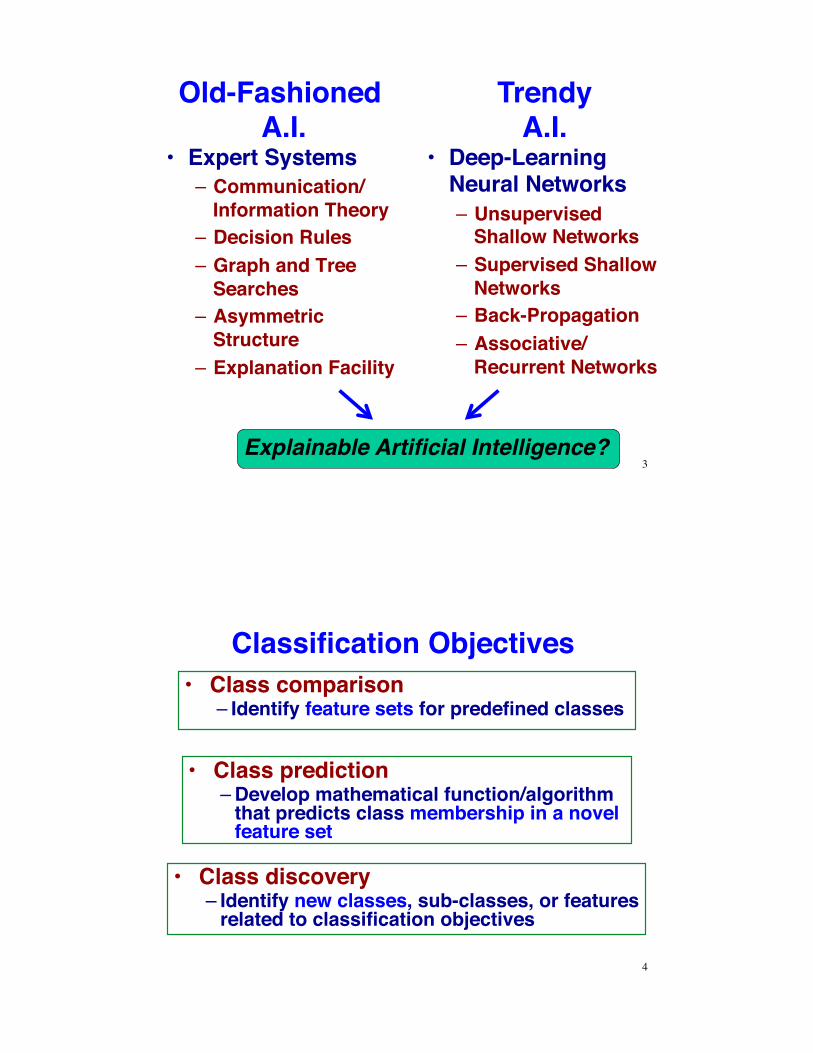
Classification Objectives •! Class comparison

–!Identify feature sets for predefined classes

•! Class prediction–!Develop mathematical function/algorithm

that predicts class membership in a novel feature set

•! Class discovery–!Identify new classes, sub-classes, or features

related to classification objectives

4

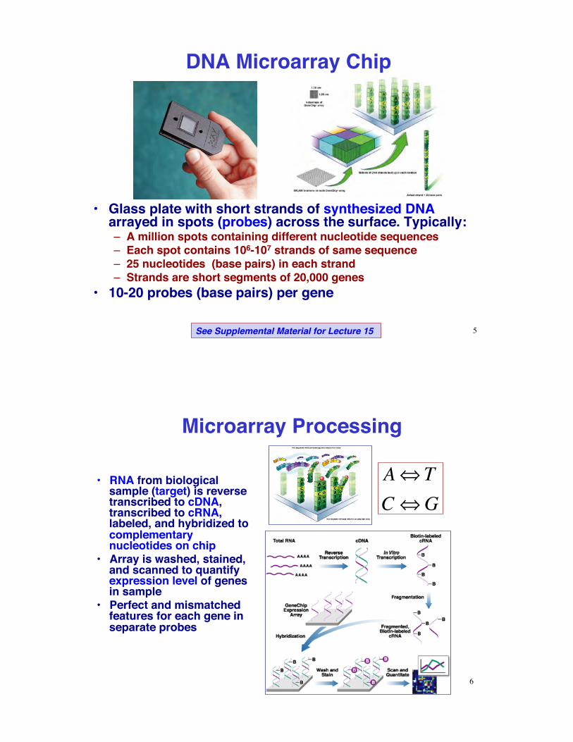
DNA Microarray Chip

5See Supplemental Material for Lecture 15

•! Glass plate with short strands of synthesized DNA arrayed in spots (probes) across the surface. Typically:–! A million spots containing different nucleotide sequences–! Each spot contains 106-107 strands of same sequence–! 25 nucleotides (base pairs) in each strand–! Strands are short segments of 20,000 genes

•! 10-20 probes (base pairs) per gene

Microarray Processing

•! RNA from biological sample (target) is reverse transcribed to cDNA, transcribed to cRNA, labeled, and hybridized to complementary nucleotides on chip

•! Array is washed, stained, and scanned to quantify expression level of genes in sample

•! Perfect and mismatched features for each gene in separate probes

6

A! TC!G

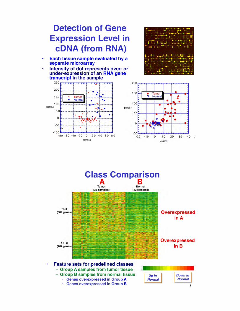
Detection of Gene Expression Level in

cDNA (from RNA)

-100

-50

0

5 0

100

150

200

250

-80 -60 -40 -20 0 2 0 4 0 6 0 8 0

TumorNormal

H57136

M96839

•! Each tissue sample evaluated by a separate microarray

•! Intensity of dot represents over- or under-expression of an RNA gene transcript in the sample

7

Class Comparison A B

Overexpressed in B

Overexpressed in A

8

•! Feature sets for predefined classes–! Group A samples from tumor tissue–! Group B samples from normal tissue

•! Genes overexpressed in Group A•! Genes overexpressed in Group B

Up In Normal

Down in Normal

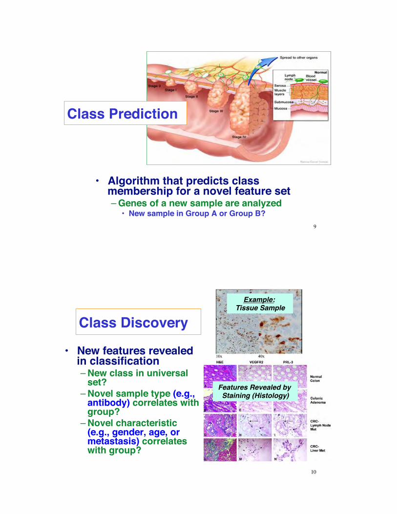
•! Algorithm that predicts class membership for a novel feature set–!Genes of a new sample are analyzed

•! New sample in Group A or Group B?

Class Prediction

9

•! New features revealed in classification–!New class in universal

set?–!Novel sample type (e.g.,

antibody) correlates with group?

–!Novel characteristic (e.g., gender, age, or metastasis) correlates with group?

Class Discovery Example:

Tissue Sample

10

Features Revealed by Staining (Histology)

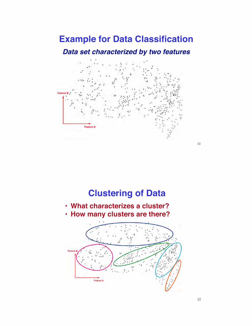
Example for Data ClassificationData set characterized by two features

11

Clustering of Data•! What characterizes a cluster?•! How many clusters are there?

12

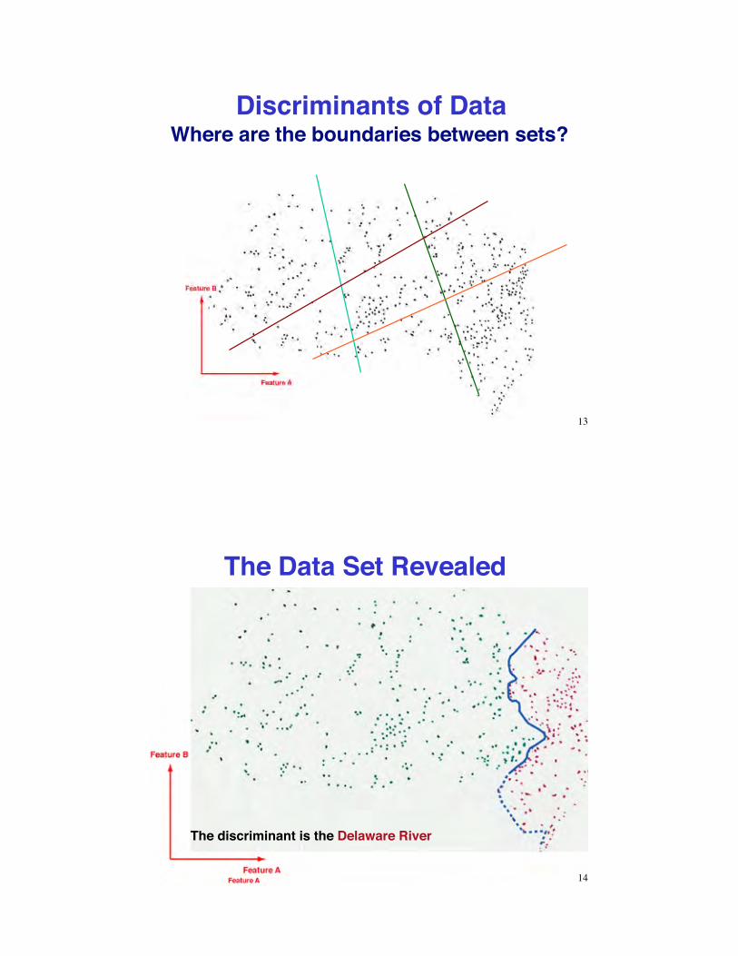
Discriminants of DataWhere are the boundaries between sets?

13

The Data Set Revealed

The discriminant is the Delaware River

14

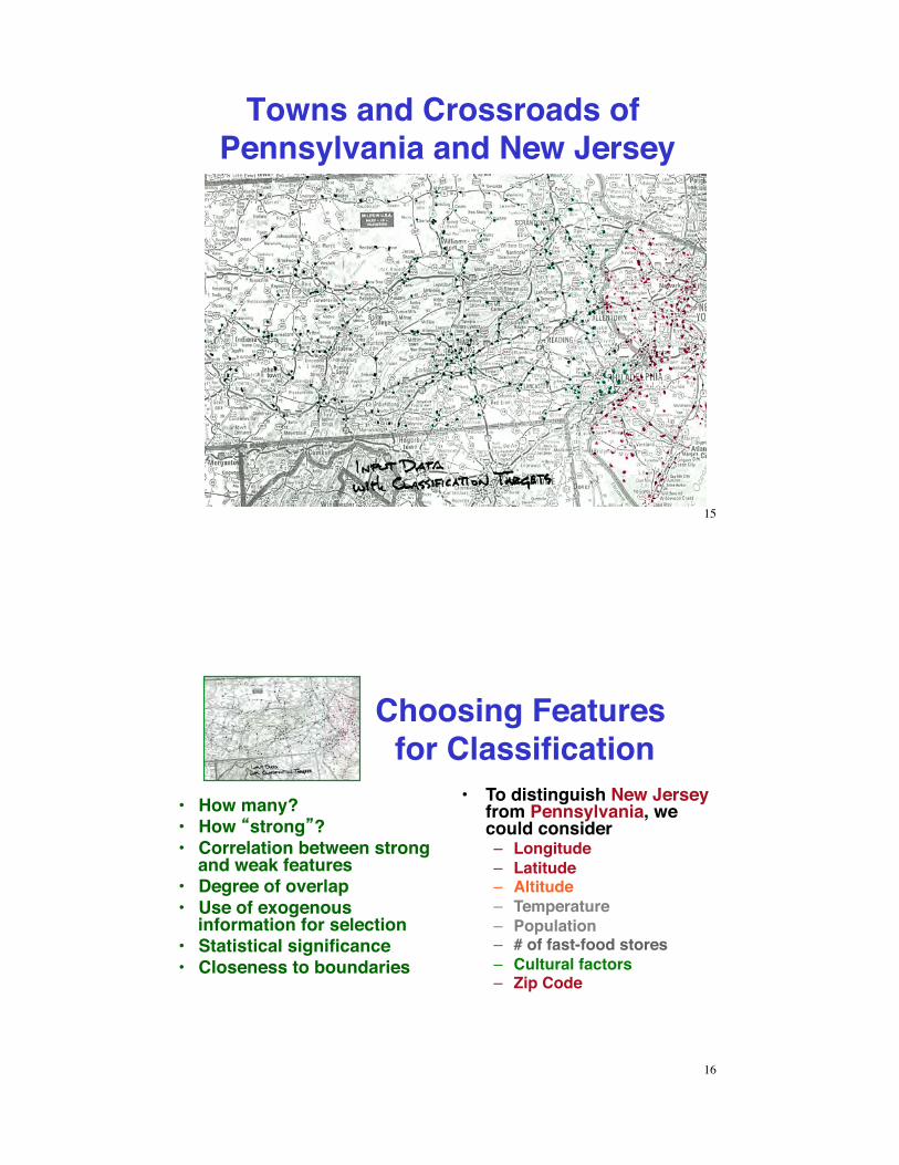
Towns and Crossroads of Pennsylvania and New Jersey

15

Choosing Features for Classification

•! How many?•! How strong ?•! Correlation between strong

and weak features•! Degree of overlap•! Use of exogenous

information for selection•! Statistical significance•! Closeness to boundaries

•! To distinguish New Jersey from Pennsylvania, we could consider–! Longitude–! Latitude–! Altitude–! Temperature–! Population–! # of fast-food stores–! Cultural factors–! Zip Code

16

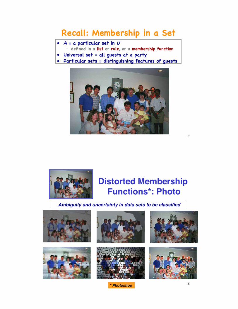
Recall: Membership in a Set!•! A = a particular set in U !

–! defined in a list or rule, or a membership function!•! Universal set = all guests at a party!•! Particular sets = distinguishing features of guests!

17

Distorted Membership Functions*: Photo

Ambiguity and uncertainty in data sets to be classified

* Photoshop 18

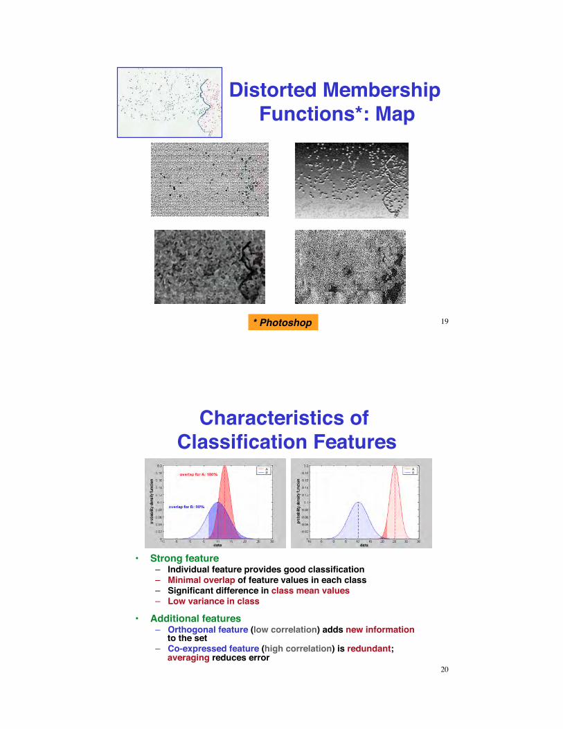
Distorted Membership Functions*: Map

* Photoshop 19

Characteristics of Classification Features

•! Additional features–! Orthogonal feature (low correlation) adds new information

to the set–! Co-expressed feature (high correlation) is redundant;

averaging reduces error

•! Strong feature–! Individual feature provides good classification–! Minimal overlap of feature values in each class–! Significant difference in class mean values–! Low variance in class

20

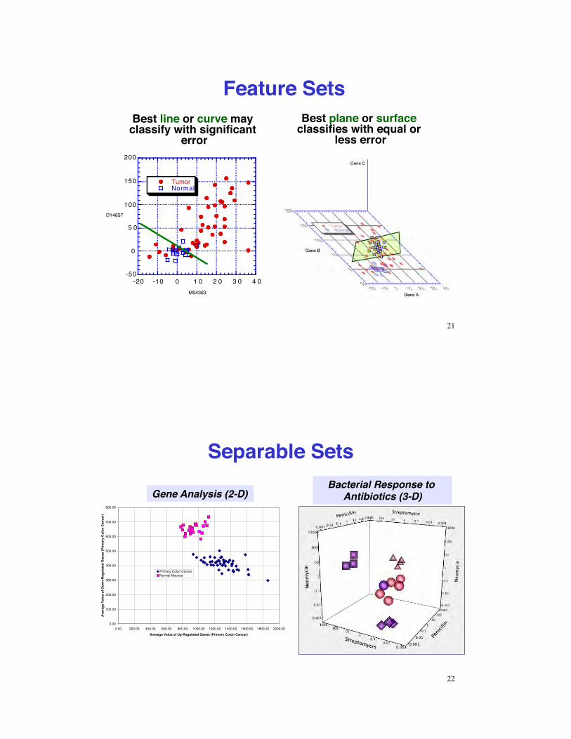
Feature Sets

-50

0

5 0

100

150

200

-20 -10 0 1 0 2 0 3 0 4 0

TumorNormal

D14657

M94363

Best line or curve may classify with significant

error

Best plane or surface classifies with equal or

less error

21

Separable Sets

0.00

100.00

200.00

300.00

400.00

500.00

600.00

700.00

800.00

0.00 200.00 400.00 600.00 800.00 1000.00 1200.00 1400.00 1600.00 1800.00 2000.00Average Value of Up-Regulated Genes (Primary Colon Cancer)

Ave

rage

Val

ue o

f Dow

n-R

egul

ated

Gen

es (P

rimar

y C

olon

Can

cer)

Primary Colon CancerNormal Mucosa

Gene Analysis (2-D)Bacterial Response to

Antibiotics (3-D)

22

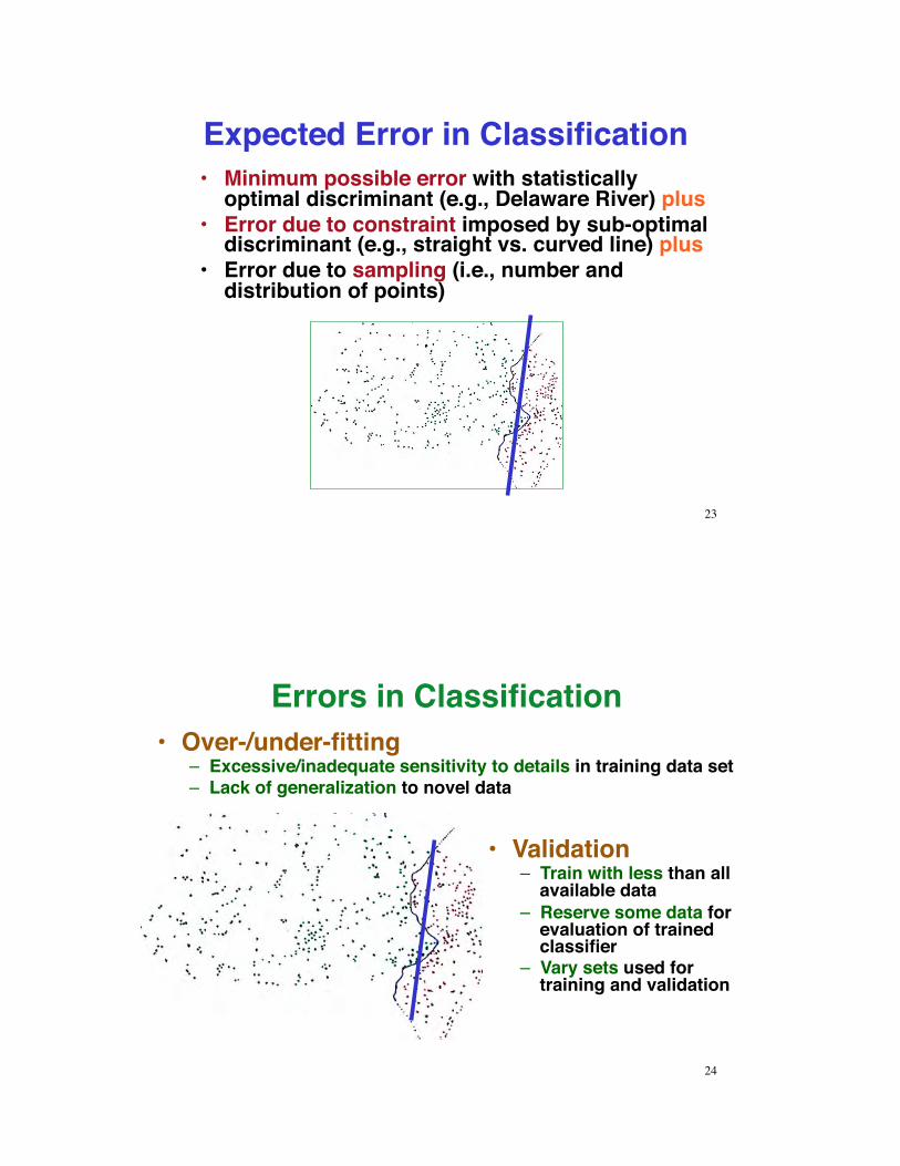
Expected Error in Classification •! Minimum possible error with statistically

optimal discriminant (e.g., Delaware River) plus•! Error due to constraint imposed by sub-optimal

discriminant (e.g., straight vs. curved line) plus•! Error due to sampling (i.e., number and

distribution of points)

23

Errors in Classification •! Over-/under-fitting

–! Excessive/inadequate sensitivity to details in training data set–! Lack of generalization to novel data

•! Validation–! Train with less than all

available data–! Reserve some data for

evaluation of trained classifier

–! Vary sets used for training and validation

24

Validation of Classifier

•! Train, Validate, and Test•! Reserve some data for evaluation of trained classifier•! Train with A, test with B

–! A: Training set (or sample)–! B: Novel set (or sample)–! Vary sets used for training and validation

•! Leave-one-out validation (combined validation and test)–! Remove a single sample–! Train on remaining samples–! Does the trained classifier identify the single sample?–! Repeat with all sets, removing all samples, one-by-one

25

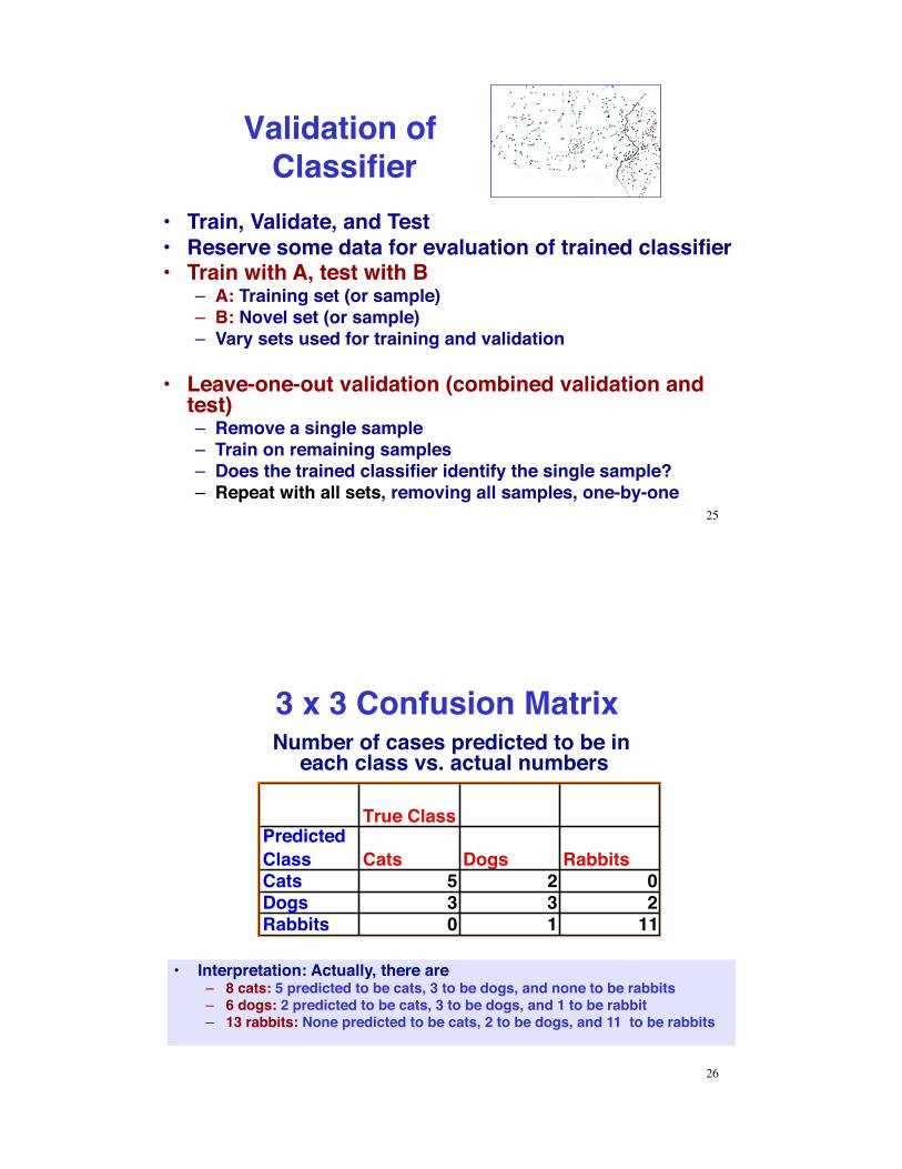
3 x 3 Confusion Matrix Number of cases predicted to be in

each class vs. actual numbers

True ClassPredicted Class Cats Dogs RabbitsCats 5 2 0Dogs 3 3 2Rabbits 0 1 11

•! Interpretation: Actually, there are–! 8 cats: 5 predicted to be cats, 3 to be dogs, and none to be rabbits–! 6 dogs: 2 predicted to be cats, 3 to be dogs, and 1 to be rabbit–! 13 rabbits: None predicted to be cats, 2 to be dogs, and 11 to be rabbits

26

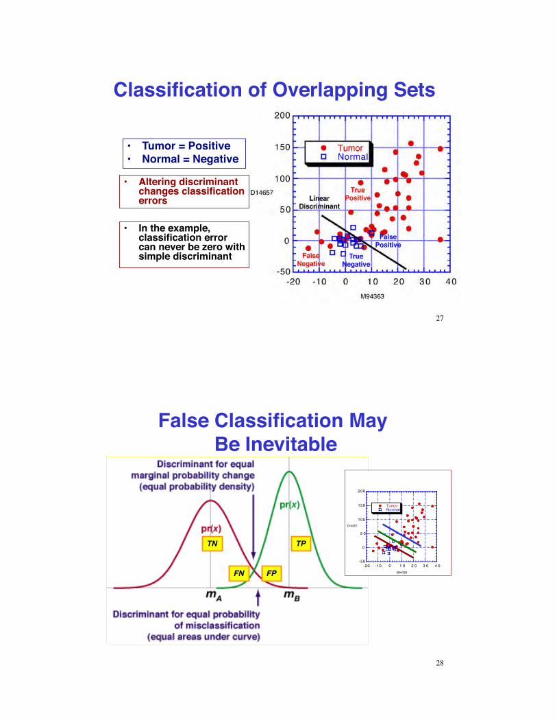
Classification of Overlapping Sets

•! Tumor = Positive•! Normal = Negative

•! Altering discriminant changes classification errors

•! In the example, classification error can never be zero with simple discriminant

27

False Classification May Be Inevitable

TP

FN FP

TN

-50

0

5 0

100

150

200

-20 -10 0 1 0 2 0 3 0 4 0

TumorNormal

D14657

M94363

28

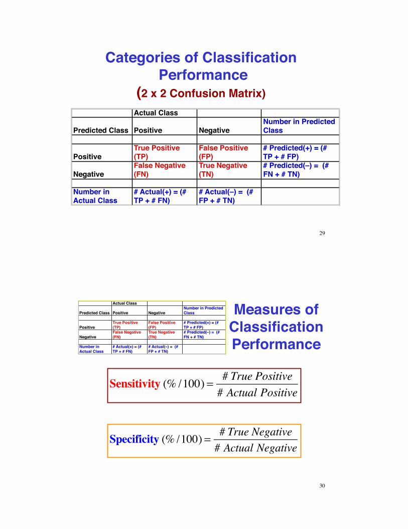
Categories of Classification Performance!

(2 x 2 Confusion Matrix) Actual Class

Predicted Class Positive NegativeNumber in Predicted Class

PositiveTrue Positive (TP)

False Positive (FP)

# Predicted(+) = (# TP + # FP)

NegativeFalse Negative (FN)

True Negative (TN)

# Predicted(–) = (# FN + # TN)

Number in Actual Class

# Actual(+) = (# TP + # FN)

# Actual(–) = (# FP + # TN)

29

Measures of Classification Performance

Specificity (% /100) = # True Negative# Actual Negative

Sensitivity (% /100) = # True Positive# Actual Positive

Actual Class

Predicted Class Positive NegativeNumber in Predicted Class

PositiveTrue Positive (TP)

False Positive (FP)

# Predicted(+) = (# TP + # FP)

NegativeFalse Negative (FN)

True Negative (TN)

# Predicted(–) = (# FN + # TN)

Number in Actual Class

# Actual(+) = (# TP + # FN)

# Actual(–) = (# FP + # TN)

30

Measures of Classification Performance

Accuracy (%/100) = # True Positive + # True Negative# Actual Positive + # Actual Negative

Positive Predictive Value (%/100) = # True Positive# Predicted Positive

Negative Predictive Value (%/100) = # True Negative# Predicted Negative

31

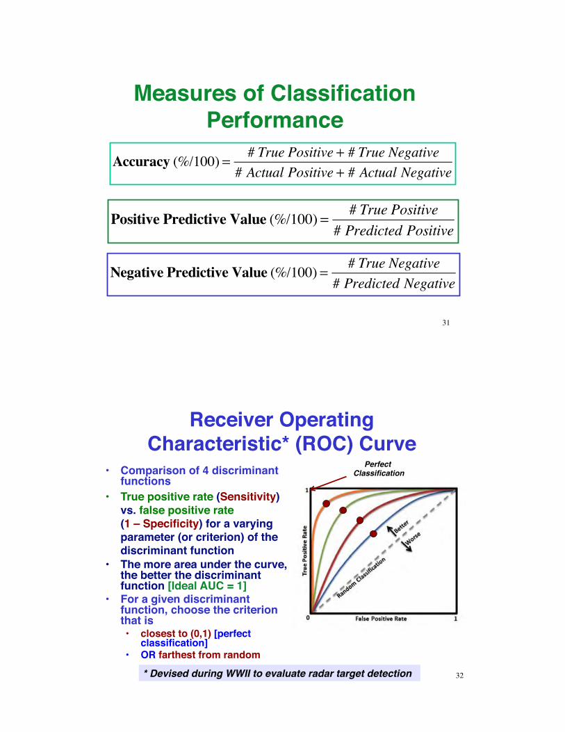
Receiver Operating Characteristic* (ROC) Curve

•! Comparison of 4 discriminant functions

•! True positive rate (Sensitivity) vs. false positive rate (1 – Specificity) for a varying parameter (or criterion) of the discriminant function

•! The more area under the curve, the better the discriminant function [Ideal AUC = 1]

•! For a given discriminant function, choose the criterion that is •! closest to (0,1) [perfect

classification] •! OR farthest from random

* Devised during WWII to evaluate radar target detection 32

Perfect Classification

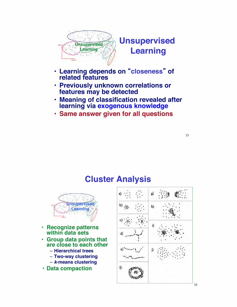
Unsupervised Learning

•! Learning depends on closeness of related features

•! Previously unknown correlations or features may be detected

•! Meaning of classification revealed after learning via exogenous knowledge

•! Same answer given for all questions

UnsupervisedLearning

33

Cluster Analysis

UnsupervisedLearning

•! Recognize patterns within data sets

•! Group data points that are close to each other–!Hierarchical trees–! Two-way clustering–! k-means clustering

•! Data compaction

34

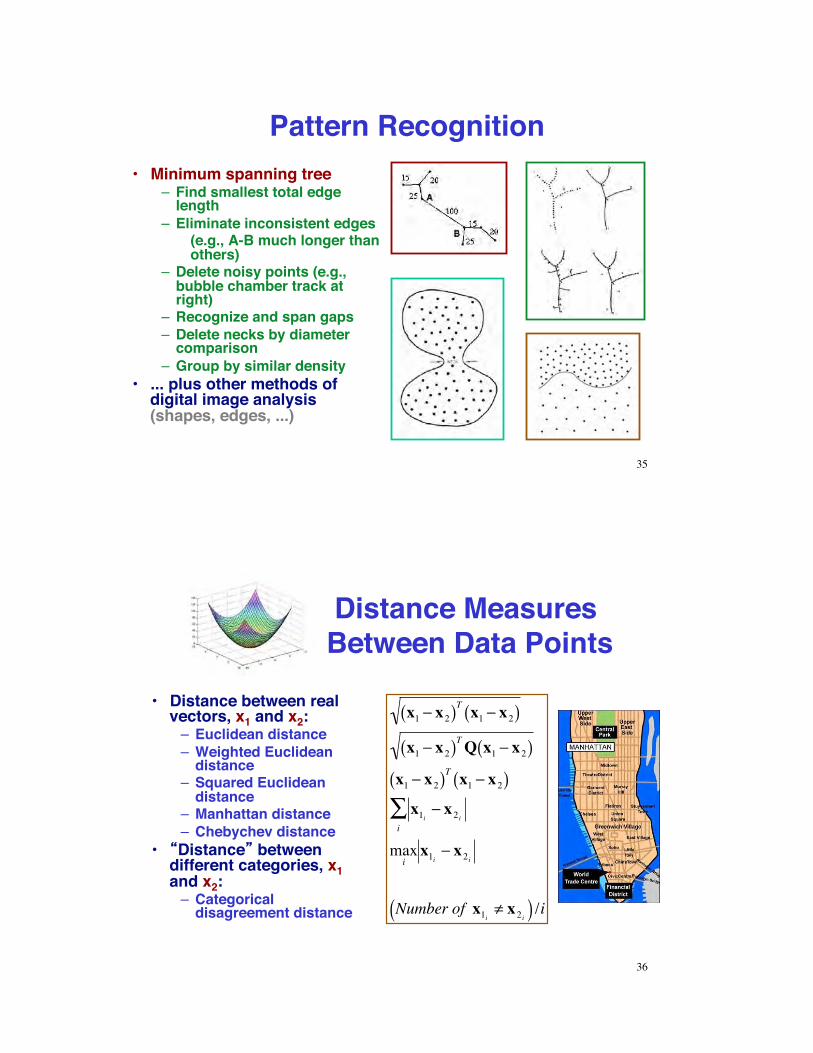
Pattern Recognition•! Minimum spanning tree

–! Find smallest total edge length

–! Eliminate inconsistent edges(e.g., A-B much longer than others)

–! Delete noisy points (e.g., bubble chamber track at right)

–! Recognize and span gaps–! Delete necks by diameter

comparison–! Group by similar density

•! ... plus other methods of digital image analysis (shapes, edges, ...)

35

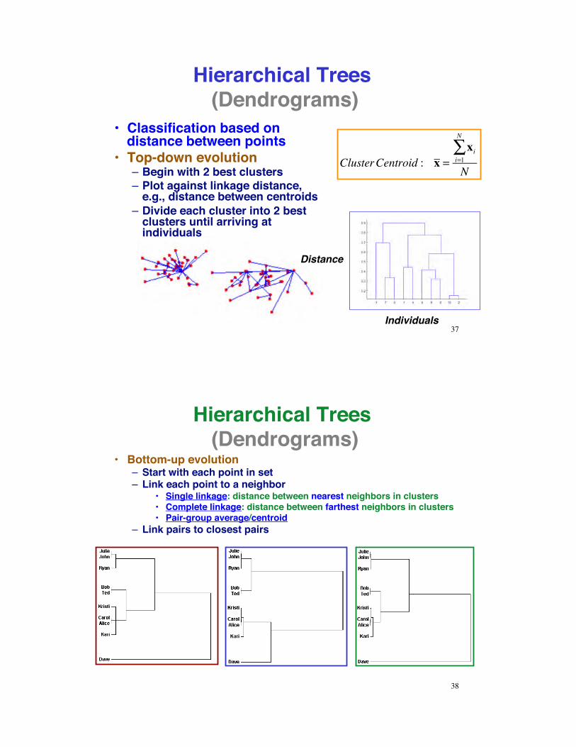
Distance Measures Between Data Points

•! Distance between real vectors, x1 and x2:–! Euclidean distance–! Weighted Euclidean

distance–! Squared Euclidean

distance–! Manhattan distance–! Chebychev distance

•! Distance between different categories, x1 and x2:–! Categorical

disagreement distance

x1 ! x2( )T x1 ! x2( )x1 ! x2( )TQ x1 ! x2( )x1 ! x2( )T x1 ! x2( )x1i ! x2 i

i"max

ix1i ! x2 i

Number of x1i # x2 i( ) /i

36

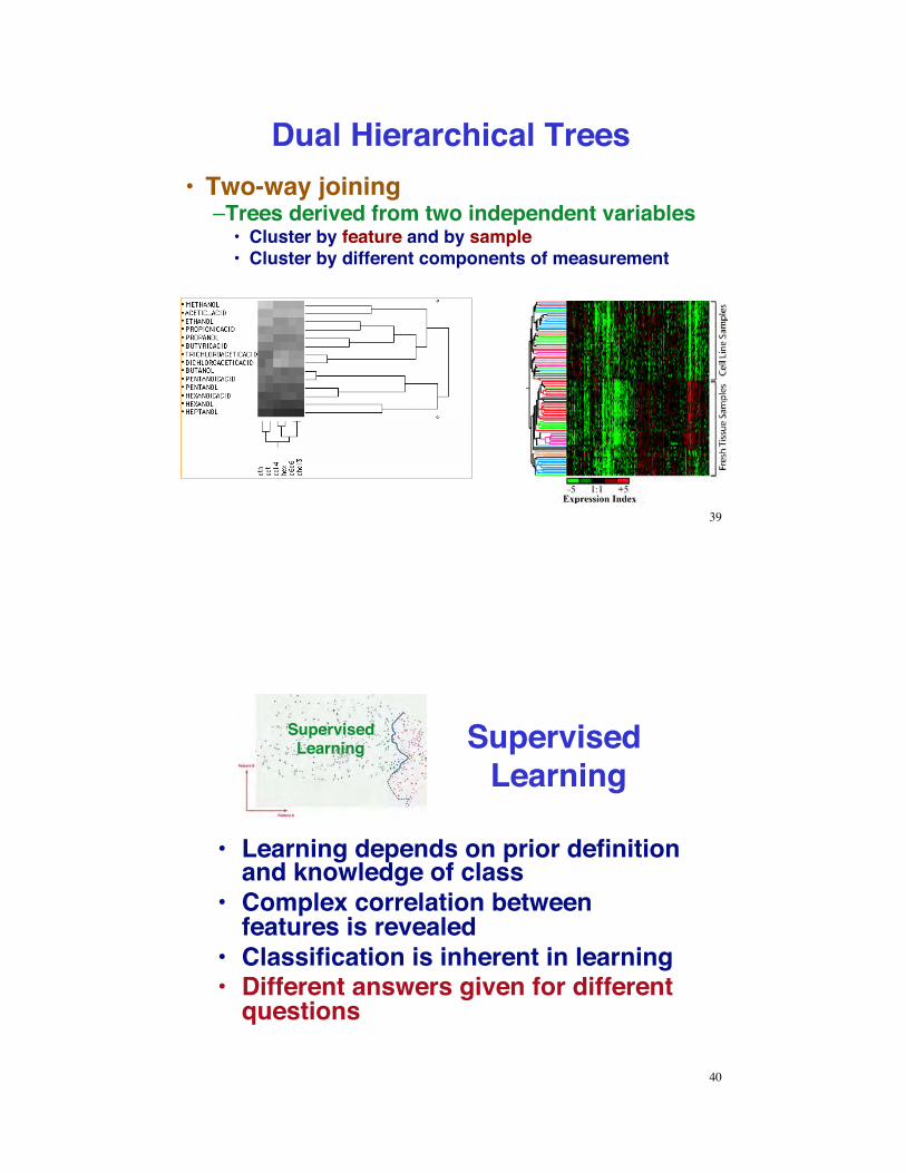
Hierarchical Trees (Dendrograms)

•! Classification based on distance between points

•! Top-down evolution–!Begin with 2 best clusters–! Plot against linkage distance,

e.g., distance between centroids–!Divide each cluster into 2 best

clusters until arriving at individuals

ClusterCentroid : x =xi

i=1

N

!N

37

Distance

Individuals

Hierarchical Trees (Dendrograms)

•! Bottom-up evolution–! Start with each point in set–! Link each point to a neighbor

•! Single linkage: distance between nearest neighbors in clusters•! Complete linkage: distance between farthest neighbors in clusters•! Pair-group average/centroid

–! Link pairs to closest pairs

38

Dual Hierarchical Trees•! Two-way joining

–!Trees derived from two independent variables•! Cluster by feature and by sample •! Cluster by different components of measurement

39

Supervised Learning

•! Learning depends on prior definition and knowledge of class

•! Complex correlation between features is revealed

•! Classification is inherent in learning•! Different answers given for different

questions

SupervisedLearning

40

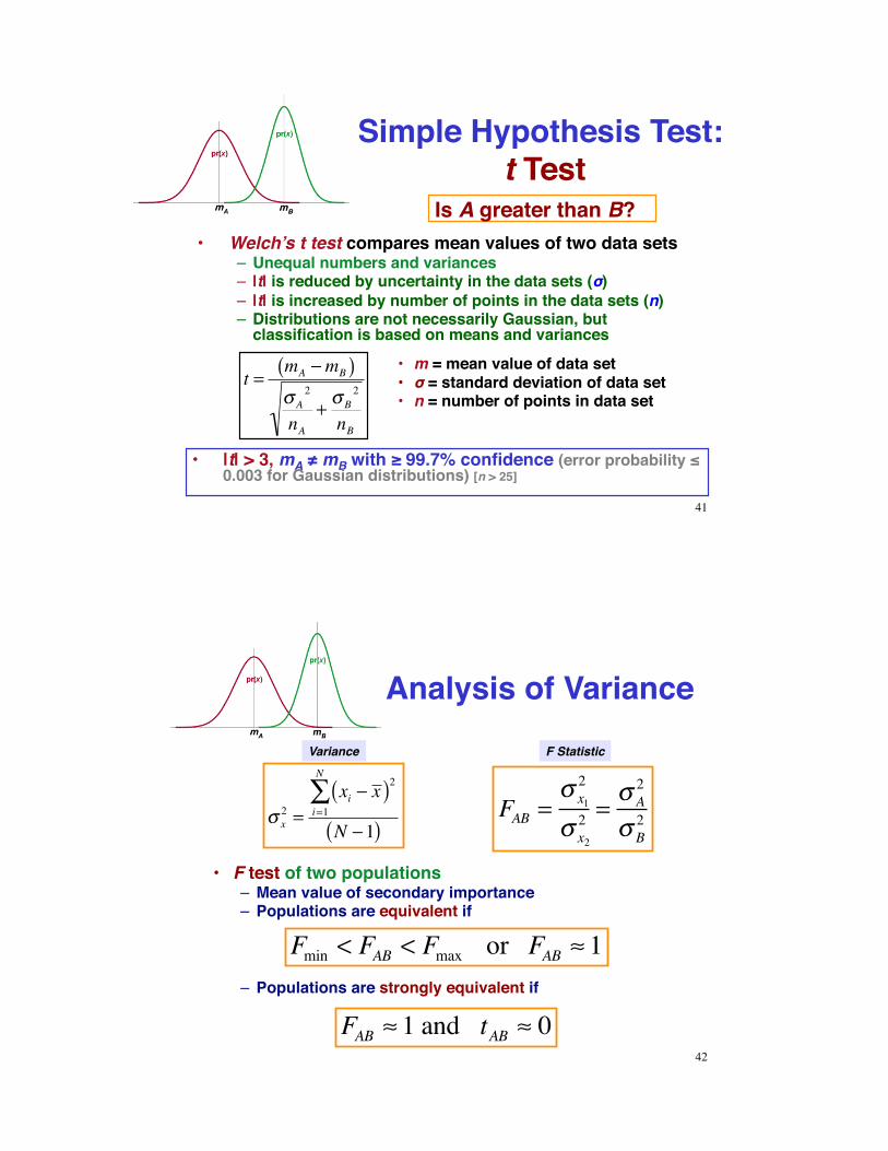
Simple Hypothesis Test: t Test

Is A greater than B?

•! m = mean value of data set•! ! = standard deviation of data set•! n = number of points in data set

•! |t| > 3, mA " mB with # 99.7% confidence (error probability $ 0.003 for Gaussian distributions) [n > 25]

•! Welch’s t test compares mean values of two data sets–! Unequal numbers and variances–! |t| is reduced by uncertainty in the data sets (!)–! |t| is increased by number of points in the data sets (n)–! Distributions are not necessarily Gaussian, but

classification is based on means and variances

t =mA !mB( )"A

2

nA+ "B

2

nB

41

Analysis of Variance

! x2 =

xi " x( )2i=1

N

#N "1( )

•! F test of two populations–! Mean value of secondary importance–! Populations are equivalent if

FAB =! x12

! x22 =

! A2

! B2

Fmin < FAB < Fmax or FAB ! 1–! Populations are strongly equivalent if

FAB ! 1 and tAB ! 0

F StatisticVariance

42

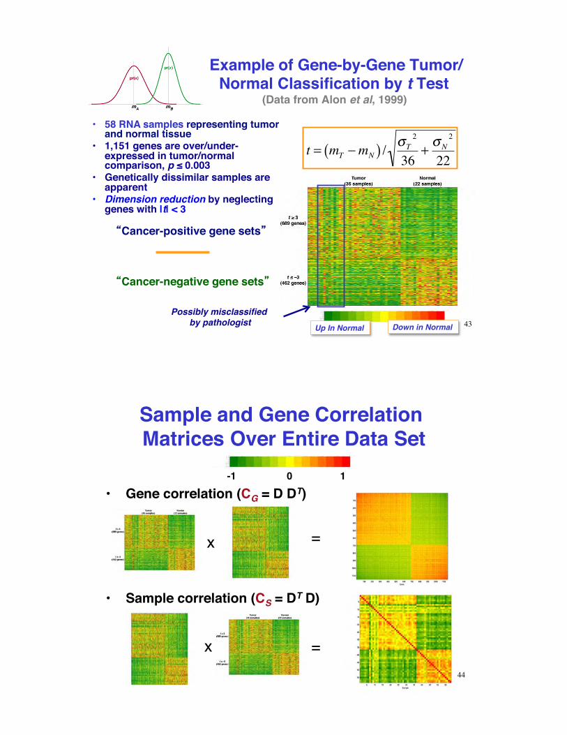
Example of Gene-by-Gene Tumor/Normal Classification by t Test

(Data from Alon et al, 1999)

t = mT !mN( ) / "T2

36+ "N

2

22

•! 58 RNA samples representing tumor and normal tissue

•! 1,151 genes are over/under-expressed in tumor/normal comparison, p $ 0.003

•! Genetically dissimilar samples are apparent

•! Dimension reduction by neglecting genes with |t| < 3

Cancer-positive gene sets

Cancer-negative gene sets

Up In Normal Down in Normal 43Possibly misclassified

by pathologist

Sample and Gene Correlation Matrices Over Entire Data Set

•! Gene correlation (CG = D DT)

x =

x =

-1 0 1

•! Sample correlation (CS = DT D)

44

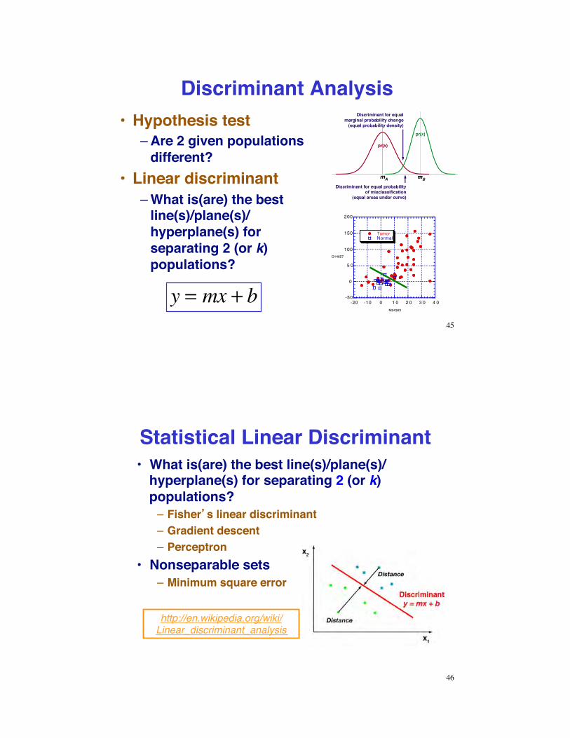
Discriminant Analysis•! Hypothesis test

–!Are 2 given populations different?

•! Linear discriminant–!What is(are) the best

line(s)/plane(s)/ hyperplane(s) for separating 2 (or k) populations?

-50

0

5 0

100

150

200

-20 -10 0 1 0 2 0 3 0 4 0

TumorNormal

D14657

M94363

y = mx + b45

Statistical Linear Discriminant•! What is(are) the best line(s)/plane(s)/

hyperplane(s) for separating 2 (or k) populations?–! Fisher s linear discriminant–!Gradient descent–! Perceptron

•! Nonseparable sets–!Minimum square error

http://en.wikipedia.org/wiki/Linear_discriminant_analysis

46

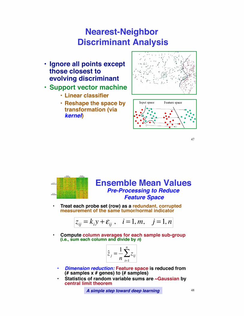
Nearest-Neighbor Discriminant Analysis

•! Ignore all points except those closest to evolving discriminant

•! Support vector machine•! Linear classifier•! Reshape the space by

transformation (via kernel)

47

Ensemble Mean Values

•! Treat each probe set (row) as a redundant, corrupted measurement of the same tumor/normal indicator

zij = kiy + !ij , i =1,m, j =1, n

ˆ z j = 1n

ziji=1

n

!•! Dimension reduction: Feature space is reduced from

(# samples x # genes) to (# samples)•! Statistics of random variable sums are ~Gaussian by

central limit theorem

•! Compute column averages for each sample sub-group (i.e., sum each column and divide by n)

48

Pre-Processing to Reduce Feature Space

A simple step toward deep learning

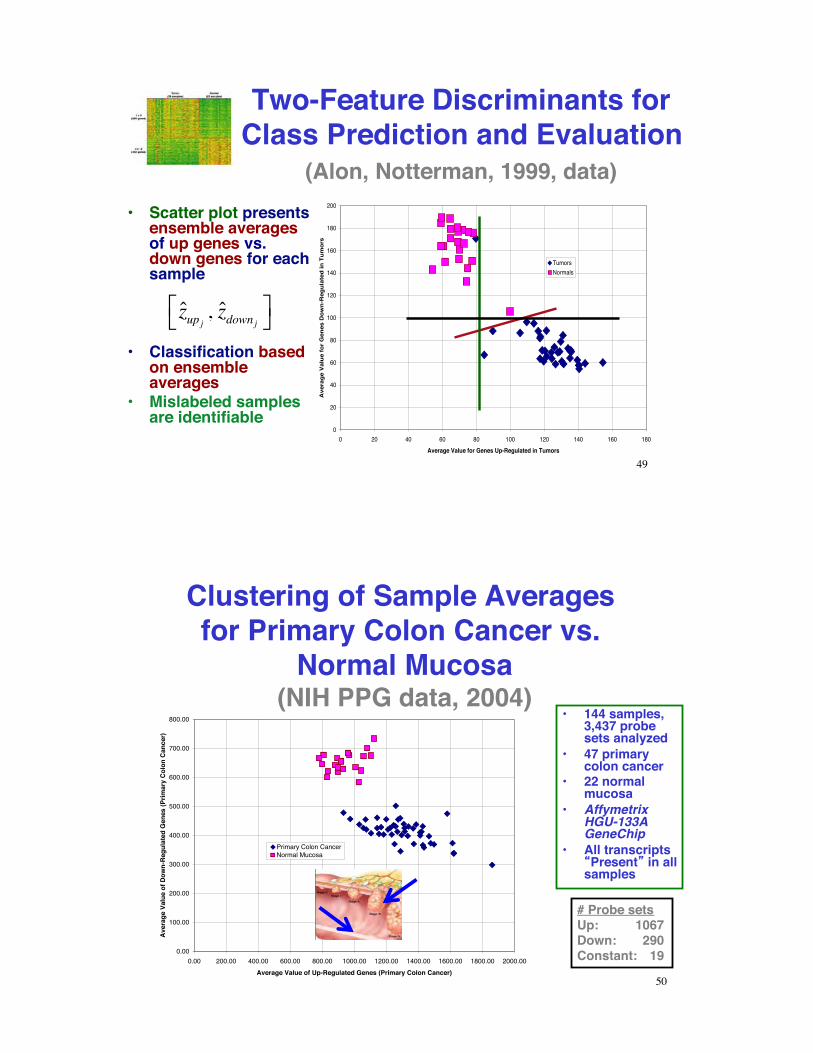
Two-Feature Discriminants for Class Prediction and Evaluation

(Alon, Notterman, 1999, data) •! Scatter plot presents

ensemble averages of up genes vs. down genes for each sample

•! Classification based on ensemble averages

•! Mislabeled samples are identifiable

zupj , zdownj!" #$

0

20

40

60

80

100

120

140

160

180

200

0 20 40 60 80 100 120 140 160 180Average Value for Genes Up-Regulated in Tumors

Ave

rage

Val

ue fo

r G

enes

Dow

n-R

egul

ated

in T

umor

s

TumorsNormals

49

Clustering of Sample Averages for Primary Colon Cancer vs.

Normal Mucosa!(NIH PPG data, 2004)

# Probe setsUp: 1067Down: 290Constant: 19

•! 144 samples, 3,437 probe sets analyzed

•! 47 primary colon cancer

•! 22 normal mucosa

•! Affymetrix HGU-133A GeneChip

•! All transcripts Present in all

samples

0.00

100.00

200.00

300.00

400.00

500.00

600.00

700.00

800.00

0.00 200.00 400.00 600.00 800.00 1000.00 1200.00 1400.00 1600.00 1800.00 2000.00Average Value of Up-Regulated Genes (Primary Colon Cancer)

Ave

rage

Val

ue o

f Dow

n-R

egul

ated

Gen

es (P

rimar

y C

olon

Can

cer)

Primary Colon CancerNormal Mucosa

50

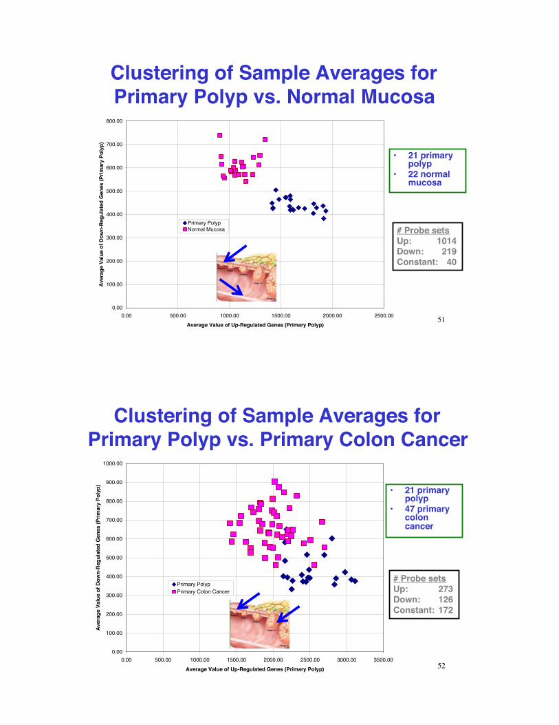
Clustering of Sample Averages for Primary Polyp vs. Normal Mucosa

0.00

100.00

200.00

300.00

400.00

500.00

600.00

700.00

800.00

0.00 500.00 1000.00 1500.00 2000.00 2500.00Average Value of Up-Regulated Genes (Primary Polyp)

Ave

rage

Val

ue o

f Dow

n-R

egul

ated

Gen

es (P

rimar

y Po

lyp)

Primary PolypNormal Mucosa # Probe sets

Up: 1014Down: 219Constant: 40

•! 21 primary polyp

•! 22 normal mucosa

51

Clustering of Sample Averages for Primary Polyp vs. Primary Colon Cancer

0.00

100.00

200.00

300.00

400.00

500.00

600.00

700.00

800.00

900.00

1000.00

0.00 500.00 1000.00 1500.00 2000.00 2500.00 3000.00 3500.00Average Value of Up-Regulated Genes (Primary Polyp)

Ave

rage

Val

ue o

f Dow

n-R

egul

ated

Gen

es (P

rimar

y Po

lyp)

Primary PolypPrimary Colon Cancer

# Probe setsUp: 273Down: 126Constant: 172

•! 21 primary polyp

•! 47 primary colon cancer

52

Next Time:!Introduction to Neural Networks!

53

SSuupppplleemmeennttaall MMaatteerriiaall

54

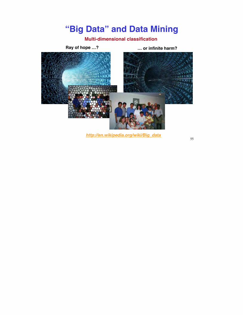
“Big Data” and Data Mining

http://en.wikipedia.org/wiki/Big_data

Ray of hope …? … or infinite harm?

Multi-dimensional classification

55