Stochastic Optimization for Operating Chemical … Optimization for Operating Chemical Processes 459...

∗Stochastic Optimization for Operating ChemicalProcesses under Uncertainty

René Henrion1, Pu Li2, Andris Möller1, Marc C. Steinbach3, Moritz Wendt2, andGünter Wozny2

1 Weierstraß-Institut für Angewandte Analysis und Stochastik (WIAS), Berlin, Germany2 Institut für Prozess- und Anlagentechnik, Technische Universität Berlin, Germany3 Konrad-Zuse-Zentrum für Informationstechnik Berlin (ZIB), Germany

Abstract Mathematical optimization techniques are on their way to becoming a standardtool in chemical process engineering. While such approaches are usually based on deter-ministic models, uncertainties such as external disturbances play a significant role in manyreal-life applications. The present article gives an introduction to practical issues of processoperation and to basic mathematical concepts required for the explicit treatment of uncertain-ties by stochastic optimization.

1 OPERATING CHEMICAL PROCESSES

Chemical industry plays an essential role in the daily life of our society. The purposeof a chemical process is to transfer some (cheap) materials into other (desired) ma-terials. Those materials include any sorts of solids, liquids and gas and can be singlecomponents or multicomponent mixtures. Common examples of chemical processesare reaction, separation and crystallization processes usually composed of operationunits like reactors, distillation columns, heat exchangers and so on. Based on mar-ket demands, those processes are designed, set up and put into operation. From thedesign, the process is expected to be run at a predefined operating point, i.e., with acertain flow rate, temperature, pressure and composition [22].

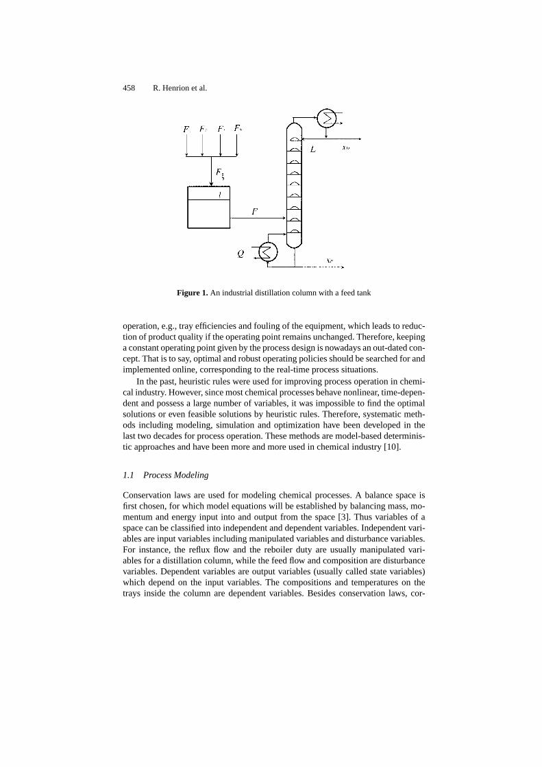
Distillation is one of the most common separation processes which consumesthe largest part of energy in chemical industry. Figure 1 shows an industrial distil-lation process to separate a mixture of methanol and water to high purity products(methanol composition in the distillate and the bottom should be xD ≥ 99.5 mol%and xB ≤ 0.5 mol%, respectively). The feed flow F to the column is from outflowsof different upstream plants. These streams are first accumulated in a tank (a middlebuffer) and then fed to the column. The column is operated at atmospheric pressure.From the design, the diameter of the column, the number of trays, the reboiler dutyQ and the reflux flow L will be defined for the given product specifications.

For an existing chemical process, it is important to develop flexible operatingpolicies to improve its profitability and reducing its effect of pollution. The ever-changing market conditions demand a high flexibility for chemical processes un-der different product specifications and different feedstocks. On the other hand,the increasingly stringent limitations to process emissions (e.g., xB ≤ 0.5 mol% inthe above example) require suitable new operating conditions satisfying these con-straints. Moreover, the properties of processes themselves change during process

458 R. Henrion et al.

Figure 1. An industrial distillation column with a feed tank

operation, e.g., tray efficiencies and fouling of the equipment, which leads to reduc-tion of product quality if the operating point remains unchanged. Therefore, keepinga constant operating point given by the process design is nowadays an out-dated con-cept. That is to say, optimal and robust operating policies should be searched for andimplemented online, corresponding to the real-time process situations.

In the past, heuristic rules were used for improving process operation in chemi-cal industry. However, since most chemical processes behave nonlinear, time-depen-dent and possess a large number of variables, it was impossible to find the optimalsolutions or even feasible solutions by heuristic rules. Therefore, systematic meth-ods including modeling, simulation and optimization have been developed in thelast two decades for process operation. These methods are model-based determinis-tic approaches and have been more and more used in chemical industry [10].

1.1 Process Modeling

Conservation laws are used for modeling chemical processes. A balance space isfirst chosen, for which model equations will be established by balancing mass, mo-mentum and energy input into and output from the space [3]. Thus variables of aspace can be classified into independent and dependent variables. Independent vari-ables are input variables including manipulated variables and disturbance variables.For instance, the reflux flow and the reboiler duty are usually manipulated vari-ables for a distillation column, while the feed flow and composition are disturbancevariables. Dependent variables are output variables (usually called state variables)which depend on the input variables. The compositions and temperatures on thetrays inside the column are dependent variables. Besides conservation laws, cor-

Stochastic Optimization for Operating Chemical Processes 459

relation equations based on physical and chemical principles are used to describerelations between state variables. These principles include vapor-liquid equilibriumif two phases exist in the space, reaction kinetics if a reaction takes place and fluiddynamics for describing the hydraulics influenced by the structure of the equipment.

Let us consider modeling a general tray of a distillation column, as shown inFigure 2, where i and j are the indexes of components (i = 1,NK) and trays (fromthe condenser to the reboiler), respectively. The dependent variables on each trayare the vapor and liquid compositions yi,j, xi,j, vapor and liquid flow rate Vj, Lj,liquid molar holdup Mj, temperature Tj and pressure Pj. The independent variablesare the feed flow rate and composition Fj, zFi,j, heat flow Qj and the flows andcompositions from the upper as well as lower tray. The model equations includecomponent and energy balances, vapor-liquid equilibrium equations, a liquid holdupequation as well as a pressure drop equation (hydraulics) for each tray of the column:

– Component balance:

d(Mjxi,j)

dt= Lj−1xi,j−1 + Vj+1yi,j+1 − Ljxi,j − Vjyi,j + FjzFi,j (1)

– Phase equilibrium:

yi,j = ηjKi,j(xi,j, Tj, Pj)xi,j + (1 − ηj)yi,j+1 (2)

– Summation equation:

NK∑i=1

xi,j = 1,

NK∑i=1

yi,j = 1 (3)

– Energy balance:

d(MjHLj )

dt= Lj−1H

Lj−1 + Vj+1H

Vj+1 − LjH

Lj − VjH

Vj + FjH

LF,j + Qj (4)

– Holdup correlation:Mj = ϕj(xi,j, Tj, Lj) (5)

– Pressure drop equation:

Pj = Pj−1 + ψ(xi,j−1, yi,j, Lj−1, Vj, Tj) (6)

In addition to the equations (1)–(6), there are auxiliary relations to describe the va-por and liquid enthalpy HV

j , HLj , phase equilibrium constant Ki,j, holdup correlation

ϕj and pressure drop correlation ψj which are functions of the dependent variables.Parameters in these correlations can be found in chemical engineering handbookslike [9, 19]. Murphree tray efficiency ηj is introduced to describe the nonequilib-rium behavior. This is a parameter that can be verified by comparing the simulationresults with the operating data.


Figure 2. A general tray of the distillation column

Equations of all trays in the column lead to a complicated nonlinear DAE sys-tem. Moreover, some dependent variables are required to be kept at a predefinedvalue (e.g., the bottom liquid level of the column). This will be realized by feed-back control loops usually with PID (proportional-integral-derivative) controllers.Thus controller equations have to be added to the model equation system, if closedloop behaviors will be studied. Process simulation means, with given independ-ent variables, to solve the DAE so as to gain the profiles of the dependent vari-ables. In the framework of optimization, an objective function will be defined (e.g.,minimizing the energy consumption during the operation). The above DAE systemwill be the equality constraints. The inequality constraints consist of the distillateand bottom product specifications as well as the physical limitations of vapor andliquid flow rates. Thus a dynamic nonlinear optimization problem is formulated.Approaches to solve dynamic optimization problems use a discretization method(either multiple-shooting or orthogonal collocation) to transform the dynamic sys-tem to a NLP problem. They can be classified into simultaneous approaches, whereall discretized variables are included in a huge NLP problem, and sequential ap-proaches, where a simulation step is used to compute the dependent variables andthus only the independents will be solved by NLP. Solution approaches to suchproblems can be found in [15, 23]. As a result, optimal operating policies for themanipulated variables can be achieved. It should be noted that some processes mayhave zero degree of freedom. In the above example, when the product specificationsbecome equalities, it implies that the independent variables at the steady state mustbe fixed for fulfilling these specifications.

1.2 Uncertainties in Process Operation

Although deterministic approaches have been successfully applied to many complexchemical processes, their results are only applicable if the real operating conditionsare included in the problem formulation. To deal with the unknown operating re-ality a priori, optimization under uncertainty has to be considered [13]. From theviewpoint of process operation there are two general types of uncertainties.


Internal Uncertainties

These uncertainties represent the unavailability of the knowledge of a process. Theprocess model is only an approximation and thus can not describe the real behav-ior of the process exactly. Internal uncertainties include the model structure and theparameter uncertainty. For the description of a chemical or a thermodynamic phe-nomenon several representations always exist. The selection of a representation forthe model leads to a structure uncertainty. Model parameters (such as parameters ofreaction kinetics and vapor-liquid equilibrium) are usually estimated from a limitednumber of experimental data and hence the model may not be able to predict theactual process [28].

External Uncertainties

These uncertainties, mainly affected by market conditions, are from outside but haveimpacts on the process. These can be the flow rate and composition of the feedstock,product specifications as well as the supply of utilities. The outlet stream from anupstream unit and the recycle stream from a downstream unit are usually uncertainstreams of the considered operating unit. For some processes which are sensitiveto the surrounding conditions, the atmospheric temperature and pressure will beconsidered as external uncertain variables.

While some uncertain variables are treated as constants during the process op-eration, there are some time-dependent uncertain variables which are dependent onthe process operating conditions. For instance, the tray efficiency of a distillationcolumn often changes with its vapor and liquid load. Another example is the uncer-tainty of the feed streams coming from the upstream plants. In these cases a dynamicstochastic optimization problem will be formulated. For such problems, rather thanindividual stochastic parameters, continuous stochastic processes should be consid-ered. Approximately, most of them can be considered as normal distributed stochas-tic processes. There may exist correlation between these variables. Operation datafrom historic records can be used to estimate these stochastic properties.

In deterministic optimization approaches the expected values of uncertain vari-ables are usually employed. In the reality the uncertain variables will deviate fromtheir expected values. Based on the realized uncertain variables a reoptimization canbe carried out to correct the results from the last iteration. For dynamic optimiza-tion, a moving horizon with N time intervals will be introduced. Figure 3 showsthe implementation of the three consecutive paces of the moving horizon. At thecurrent horizon k only the values of the available policies for the first time intervalu1 which were developed in the past horizon k − 1, will be realized to the process.During this time interval a reoptimization is carried out to develop the operatingpolicies for the future horizon k + 1. The method in which the expected values ofthe uncertainties are used in the problem formulation is the so-called wait-and-seestrategy. The shortcoming of this strategy is that it can not guarantee holding in-equality constraints.


Figure 3. Reoptimization over a moving horizon

1.3 Distillation Column Operation under Uncertain Feed Streams

Now we consider again the industrial distillation process. The flows from the up-stream plants often change considerably due to the varying upstream operation. Wemay have high flow rates of the feed during the main working hours and decreasedflow rates during the night hours or at the weekend. Figure 4 shows the measuredprofiles of the total feed flow, composition and temperature for 24 hours. Here weonly focus on the impact of the variation of the flow rate. One consequence resultedfrom the fluctuating feed streams is that the tank level l may exceed the upper boundlmax (then a part of the liquid must be pumped out to an extra tank) or fall belowthe lower bound lmin (then a redundant feed stream must be added to the feed flow).Since the appearance of these cases will lead to considerable extra costs, a carefulplanning for the operation should be made to prevent these situations.

Another consequence of a large feed change is that it causes significant vari-ations of the operating point of the distillation column. To guarantee the productquality (xD, xB), a conservative operating point is usually used for a higher puritythan the required specification. This leads, however, to more energy consumptionthan required. The growth of energy requirement for a column operation is verysensitive to the product purity, especially for a high purity distillation.

Conventionally a feedback control loop is used in process industry to keep thelevel of the feed tank, using the outflow as the manipulated variable. The drawbackof this control loop is that it can not guarantee the output constraints and it willpropagate the inflow disturbance to the downstream distillation column.

To describe the continuous uncertain inflow this stochastic process will be dis-cretized as multiple stochastic variables in fixed time intervals. We assume they havea multivariate normal distribution with an available expected profile and a covari-ance matrix in the considered time horizon. The reason for this assumption is thatthe total feed of the tank is the sum of several independent streams from the up-stream plants. According to the central limit theorem [16], if a random variable isgenerated as the sum of effects of many independent random parameters, the distri-bution of the variable approaches a normal distribution, regardless of the distribution


Figure 4. Measured feed profiles of an industrial methanol-water distillation process

of each individual parameter. These parameters can be readily obtained by analyz-ing daily measured operating data. It is obvious that a wait-and-see strategy is notappropriate to be used in this process. Setting the feed flow with its expected profilein a deterministic optimization can not guarantee holding the tank level in the de-sired region. The product specification will also be easily violated by the drasticallychanging real feed flow. Therefore, a here-and-now strategy, which includes the un-certainties in the optimization problem, should be used. This will be discussed inthe next sections.

2 MODELING UNCERTAINTY

As discussed in the previous section, a common technique of correcting randomdisturbances in chemical processes is moving horizon control (or model predictivecontrol): states are measured (or estimated) in relatively small intervals, and optimalopen-loop strategies are computed over a given planning horizon—“optimal” underthe simplifying assumption that no further disturbances occur. In effect, the frequentrepetition of this process implicitly generates a (possibly nonlinear) feedback con-troller that reacts to the measured disturbances.

The stochastic approaches described here are naturally applicable within sucha moving horizon framework but differ in a fundamental aspect: rather than justreacting they look ahead by taking stochastic information on future events explicitlyinto account. This is possible if it is known which random events may occur and how


likely they are. In other words, a stochastic model of the disturbances is required,taking the form of a random process ξ = (ξt)t∈[0,T ] defined on some underlyingprobability space (Ω,F , P). Here T is the length of the planning horizon and 0 is thecurrent time. In the present context, only R

k-valued discrete-time processes for t =0, 1, . . . , T are considered, and it is assumed that ξt is observed just before time t

so that ξ0 is known at t = 0. Thus, the processes can be seen as random variablesξ = (ξ1, . . . , ξT ) in R

kT . Moreover, we consider either discrete distributions Pξ ordistributions with a continuous density function on R

kT . (More details will be givenbelow.) For a comprehensive treatment of the measure-theoretic and probability-theoretic foundations see, e.g., Bauer [1, 2].

Apparently the explicit modeling of uncertainty adds information to the opti-mization model and allows for more robust process control. The price one has topay is the necessity of solving a stochastic optimization problem whose complexitymay exceed the complexity of the underlying deterministic problem by orders ofmagnitude.

The precise nature of uncertainties (such as the time dependence and the signif-icance in objective and constraints) leads to different classes of stochastic optimiza-tion models; we will describe two of them. The first approach yields a multistagerecourse strategy consisting of optimal reactions to every observable sequence ofrandom events. It minimizes expected costs while satisfying all constraints. This isappropriate if feasible solutions exist for every possible disturbance, or if costs forthe violation of soft constraints can be quantified (as penalty terms). The secondapproach yields a single control strategy that does not react to random events but isguaranteed to satisfy the constraints with a prescribed probability. This is appropri-ate if constraint violations are unavoidable in certain extreme cases, or if they causesignificant costs that cannot be modeled exactly. For detailed discussions of stochas-tic modeling aspects and problem classes we refer to the textbooks [5] and [14].

3 SCENARIO-BASED STOCHASTIC OPTIMIZATION

In scenario-based optimization, uncertainty is modeled as a finite set of possiblerealizations of the future with associated positive probabilities. Each realization iscalled a scenario and represents a certain event or, in our case, history of events. Inprecise probabilistic terms this corresponds to a discrete distribution given by a finiteprobability space (Ω,F , P), |Ω| = N. One may simply think of ω as the “number”of a scenario, which is often emphasized by using index notation. Thus, each ele-mentary event ω ∈ Ω labels a possible realization ξω = (ξω1, . . . , ξωT ), and thedistribution is given by N probabilities (pω)ω∈Ω, that is, Pξ(ξω) = P(ω) = pω.(The σ-field is then simply the power set of the sample space, F = 2Ω.)

3.1 Scenario Trees

As indicated, we have to deal with event histories rather than single events. Thismeans that there is a finite number of realizations of ξ1, each of which may lead to


LT ≡ L2 = 3, 4, 5

L1 = 1, 2

L0 = 0

1

0

2

4 53 F2 ≡ FT = σ(3, 4, 5)

F1 = σ(3, 4, 5)

F0 = σ(3, 4, 5)

Figure 5. A small scenario tree with level sets and corresponding σ-fields

a different group of realizations of ξ2, and so on. The repeated branching of partialevent histories ξt := (ξ0, . . . , ξt), called stage t scenarios, defines a scenario tree(or event tree) whose root represents ξ0, the known observation at t = 0, and whoseleaves represent the complete set of scenarios. Thus any node represents a groupof scenarios that share a partial history ξt. We denote by V the set of nodes (orvertices) of the tree, by Lt ⊆ V the level set of nodes at time t, and by L ≡ LT

the set of leaves; further by 0 ∈ L0 the root, by j ∈ Lt the “current” node, byi ≡ π(j) ∈ Lt−1 its unique predecessor (if t > 0), and by S(j) ⊆ Lt+1 its set ofsuccessors. The scenario probabilities are pj > 0, j ∈ L. All other nodes also havea probability pj satisfying pj =

∑k∈S(j) pk. Hence,

∑j∈Lt

pj = 1 holds for all t,and p0 = 1.

Seen as a partitioning of the scenarios into groups, each level set Lt consists ofatoms generating a sub-σ-fieldFt = σ(Lt) ⊆ F (whereF0 = ∅,Ω andFT = F),and ξt is measurable with respect to Ft. The tree structure is thus reflected by thefact that these σ-fields form a filtration F0 ⊆ · · · ⊆ FT to which the process(ξt)

Tt=0 is adapted. For instance, in Figure 5 the nodes represent scenario sets as

follows: 0 ↔ 3, 4, 5, 1 ↔ 3, 4, 2 ↔ 5, 3 ↔ 3, 4 ↔ 4, and 5 ↔ 5.Since these abstract probability-theoretic notions are unnecessarily general for ourpurposes, we will use the more natural concept of scenario trees in the following.The notation ξt = (ξj)j∈Lt or ξ = (ξj)j∈V refers to the distinct realizations of ξ onlevel t or on the entire tree, respectively. (Here we include the deterministic initialevent ξ0 in ξ.)

3.2 Multistage Stochastic Programs

The main topic of this section are multistage decision processes, that is, sequencesof alternating decisions and observations over the given planning horizon. The ini-tial decision must be made without knowledge of the actual realizations of futureevents; hence it is based solely on ξ0 and the probability distribution of ξ. As thefuture unfolds, the decision maker observes realizations ξj of random events ξt,thus collecting additional information which he or she takes into account from thenon. The resulting sequence of decisions is therefore called nonanticipative. For in-stance, in controlling the feed tank of the distillation column in Section 1, we haveto decide in each time step how much liquid to extract during the next period basedon observations of the inflow during all previous periods and taking into accountthe probability distribution of future inflows. (For the initial decision, past obser-


vations do not appear explicitly in the problem but are implicitly modeled in thedistribution.)

The specific class of problems considered here are (convex quadratic) multistagerecourse problems on scenario trees, with decision vectors yj ∈ R

n, j ∈ V . Givenare convex quadratic objective functions

φj(yj) :=1

2y∗jHjyj + f∗jyj,

and polyhedral feasible sets depending on the previous decision yi ≡ yπ(j),

Y0 := y0 ≥ 0 : W0y0 = h0 , (7)

Yj(yi) := yj ≥ 0 : Wjyj = hj − Tjyi , j ∈ V∗ := V \ 0. (8)

These are the realizations of random costs φt(yt) and random sets Yt(yt−1), thatis, we take as random events the problem matrices and vectors

ξj = (Hj, fj,Wj, hj, Tj)

or, more generally, the functions and sets ξj = (φj, Yj). (Conceptually we are thusallowing entirely random problem data. In practice, however, only a subset of matrixand vector elements will usually depend on an even smaller number of randominfluences.) Decisions yj are to be made so as to minimize the immediate costsplus the expected costs of (optimal) future decisions; this is expressed in the generalmultistage recourse problem

miny0∈Y0

φ0(y0)

+ EL0

[min

y1∈Y1(y0)φ1(y1) + · · ·+ ELT−1

[min

yT∈YT (yT−1)φT (yT )

]. . .

]. (9)

Here ELt denotes the conditional expectation with respect to Lt,

ELt(Xt+1) =

∑k∈S(j)

pk

pj

Xk

j∈Lt

.

The recourse structure of this class of stochastic programs is induced by thestage-coupling equations in (8); it is best seen in the deterministic equivalent form.Defining QT+1(yT ) := 0 and then recursively

Qt(yt−1) := ELt−1

[min

yt∈Yt(yt−1)φt(yt) +Qt+1(yt)

], t = T(−1)1,

or, in terms of the realizations,

Qt(yi) :=∑

j∈S(i)

pj

pi

[min

yj∈Yj(yi)φj(yj) +Qt+1(yj)

], t = T(−1)1, i ∈ Lt−1,


the deterministic equivalent problem reads

miny0∈Y0

φ0(y0) +Q1(y0).

This has the form of a deterministic optimization problem (hence the name), butQ1 is nonlinear and in general non-smooth, so it is not necessarily an appropriateformulation for numerical computations. In the case of interest one can actuallyunwrap the nesting of minimizations to obtain a single objective; the deterministicequivalent then takes the form of a large but structured convex quadratic program inthe decision variables y = (yj)j∈V ,

miny

∑j∈V

pj

[1

2y∗jHjyj + f∗jyj

], (10)

s.t. W0y0 = h0, (11)

Wjyj = hj − Tjyi ∀j ∈ V∗, (12)

yj ≥ 0 ∀j ∈ V. (13)

This is called the extensive form. In stochastic notation with y = (y0, . . . , yT ) thesame problem reads

miny

T∑t=0

E

[1

2y∗tHtyt + f∗tyt

](14)

s.t. W0y0 = h0, (15)

Wtyt = ht − Ttyt−1 ∀t ∈ 1, . . . , T , (16)

yt ≥ 0 ∀t ∈ 0, . . . , T . (17)

Problem (14–17) and its deterministic equivalent (10–13) represent a standardproblem class in stochastic programming. Especially the linear case with fixed re-course (i.e., objective

∑t E[f∗tyt] and deterministic Wt) is very well-understood

and widely used in practice. An important property of the deterministic equivalentis that, except for the recourse sub-structure, it has the form of a standard mathe-matical program (LP, QP, CP, or NLP). Thus, even though the scenario tree maycause exponential growth of the problem size, standard solution approaches are ap-plicable when combined with suitable techniques that exploit the sparsity inducedby the stochastic nature. The most prominent such techniques are decompositionapproaches which split the large stochastic program into smaller problems associ-ated with clusters of nodes (or scenarios). For a discussion of these techniques werefer the reader to the excellent survey articles [4, 21]; our own approach combinesinterior point methods with specially developed sparse-matrix techniques.

3.3 Dynamic Structure

The stage-coupling equations (16) or (12) define (implicitly) an underlying dynamicprocess, usually combined with further equality constraints. More precisely, the


rows of conditions (16) can be categorized into dynamic equations and certain typesof constraints which possess natural interpretations and satisfy associated regularityconditions. In [25, 26] we have developed complete such categorizations for sev-eral formulations of stochastic programs, accompanied by solution algorithms thatemploy natural pivot orders resulting from the refined sparse structure.

In processes governed by differential (or difference) equations there is typicallyalso a natural partitioning of the decision variables y = (x, u) into (independent)control variables u and (dependent) state variables x, the former representing theactual degrees of freedom available to the decision maker. The dynamic equationsare then often given in explicit form,

xj = Gjxi + Ejui + hj, (18)

which is equivalent to (12) if we define Wj := (I 0) and Tj := −(Gj Ej). Inthis notation (and with the convention xπ(0), uπ(0) ∈ R

0), the multistage stochasticprogram of interest takes the form

min(x,u)

∑j∈V

pj

[1

2

(xjuj

)∗(Hj J∗jJj Kj

)(xjuj

)+

(fjdj

)∗(xjuj

)], (19)

s.t. xj = Gjxi + Ejui + hj ∀j ∈ V, (20)

x ∈ [xmin, xmax], (21)

u ∈ [umin, umax], (22)∑j∈V

pj(Fjxj + Djuj + ej) = 0. (23)

Apart from the form of dynamic equations, the major difference to the standardformulation consists in the additional equality constraint (23). This condition rep-resents a sum of expectations; we call it a global constraint since it may couple allnodes of the tree. In the standard formulation (10–13), such a condition cannot bemodeled directly; it would require surplus variables and additional constraints.

The natural interpretation of the dynamics (18) is that the decision ui at timet−1 controls all subsequent states xj, j ∈ S(i), at time t. This is the typical situationin discretized continuous-time processes: actually ui determines a control action forthe entire interval (t − 1, t) which becomes effective in xj one period later. In otherapplication contexts (particularly in the financial area), decisions become effectiveimmediately, leading to dynamic equations

xj = Gjxi + Ejuj + hj. (24)

Here each state xj has “ its own” control uj rather than sharing ui with the siblingsS(i).

The problem classes and solution algorithms associated with the possible formu-lations of dynamics are closely related; we refer to them collectively as tree-sparse.(For details see [24–26].) Applications are not only in discrete-time deterministicand stochastic optimal control but also in other dynamic optimization problems with


an underlying tree topology; extensions to network topologies with “ few” cycles arestraightforward. A very general related problem class is investigated in [20] usinga similar formulation of dynamics but σ-fields and probability spaces rather thanscenario trees.

3.4 Convex Programs

Since we are concerned with convex quadratic stochastic programs, we recall heresome basic definitions and facts of convex optimization. A convex optimizationproblem has the general form

miny∈Y

f(y) (25)

where Y is a convex set and f : Y → R is a convex function, that is,

(1 − t)y0 + ty1 ∈ Y and f((1 − t)y0 + ty1) ≤ (1 − t)f(y0) + tf(y1)

for all y0, y1 ∈ Y and t ∈ [0, 1]. A convex program (CP) is the special case

miny

f(y) s.t. g(y) = 0, h(y) ≥ 0, (26)

where g : Rn → R

m is an affine mapping, g(y) ≡ Ay + a, and h : Rn → R

k is a(component-wise) concave mapping. If f, g, h are twice continuously differentiable,this means that the Hessians of f and −hi are positive semidefinite, D2f(y) ≥ 0

and D2hi(y) ≤ 0. The convex quadratic case (with H ≥ 0) reads

miny

1

2y∗Hy + f∗y s.t. Ay + a = 0, By + b ≥ 0. (27)

The feasible set Y is a polyhedron if and only if it is given by finitely many linearequalities and inequalities, as in (27). It is easily seen that all level sets Nc := y ∈Y : f(y) ≤ c of (25) are convex. Moreover, every local solution is automatically aglobal solution, and the set S of all solutions is convex. In the general case S may beempty even if feasible solutions exist. This happens either if f is unbounded below,infy∈Y = −∞, or if f is bounded below but the level sets Nc are unbounded forc ↓ infy∈Y > −∞. Both situations are impossible in the convex quadratic case (27):existence of a solution y ∈ Y is then always guaranteed (unless the problem isinfeasible). Uniqueness of a solution y holds under standard conditions. For theconvex QP (27), a sufficient condition is positive definiteness of H on the null spaceN(A) or, more generally, on its intersection with the null spaces of the rows of B

associated with strictly active inequalities at y. All this applies in particular to thestochastic problems (10–13) and (19–23). For an exhaustive treatment of the theoryand numerical aspects of convex and (nonconvex) nonlinear programming we referthe reader to standard textbooks, such as [7, 8, 17].


4 STOCHASTIC OPTIMIZATION UNDER PROBABILISTIC CONSTRAINTS

An important instance of optimization problems with uncertain data occurs if theconstraints depend on a stochastic parameter, such as the inequality system

h(x, ξ) ≥ 0, (28)

where h : Rn ×R

s → Rm, ξ is an s-dimensional random variable defined on some

probability space (Ω,A, P) and the inequality sign has to be understood component-wise. Written as such, the constraint set is not a well-defined part of an optimizationproblem since, usually, the decision on the variables x has to be taken before ξ

can be observed. It is clear that, in order to arrive at an implementable form of theconstraints, one has to remove in an appropriate way the dependence of h on specificoutcomes of ξ. The most prominent approaches to do so are

– the expected value approach– the compensation approach– the worst case approach– the approach by probabilistic constraints

Using expected values, the system (28) is replaced by E h(x, ξ) ≥ 0, which nowcan be understood as an inequality system depending on x only, as the expectationoperator acts as an integrator over ξ. An even simpler form is obtained when therandom variable itself is replaced by its expectation: h(x, Eξ) ≥ 0 (both forms co-incide in case that h depends linearly on ξ). The last form corresponds to the naiveidea of substituting random parameters by average values. It seems obvious (andwill be demonstrated later) that such reduction to first moment information ignoressubstantial information about ξ. Indeed, the expectation approach guarantees theinequality system to be satisfied on the average only, but a decision x leading to afailure of a system for about half of the realizations of ξ is usually considered asunacceptable. On the other extreme, the worst case approach enforces a decision tobe feasible under all possible outcomes of ξ: h(x, ξ) ≥ 0 ∀ξ. This puts emphasison absolute safety which is frequently either not realizable in the strict sense or isbought by extreme increase of costs. Although diametrically opposed in their mod-eling effects, both the expected value and worst case approach share some ignoranceof the stochastic nature of ξ.

The basic idea of compensation relies on the possibility to adjust constraint vi-olations in the system (28) after observation of ξ by later compensating actions.Accordingly, the set of variables splits into first stage decisions x (to be fixed beforerealization of ξ) and second stage decisions y (to be fixed after realization of ξ).As an example, one may think of power scheduling where an optimal load patternof power generating units has to be designed prior to observing the unknown de-mand, and, where possible later gaps between supply and demand can be correctedby additional resources (e.g., hydro-thermal units, contracts etc.). The adjustment ofconstraint violation is modeled by an inequality system H(x, ξ, y) ≥ 0, connectingall three types of variables and it causes additional costs g(y, ξ) for the second stage


decisions. Of course, given x and ξ, y should be chosen as to minimize second stagecosts among all feasible decisions. Summarizing, compensation models replace theoriginal problem

min f(x) | h(x, ξ) ≥ 0

of minimizing the costs of first stage decision under stochastic inequalities by aproblem where the sum of first stage costs and expected optimal second stage costsis minimized:

minf(x) + Q(x), Q(x) = Eq(x, ξ), q(x, ξ) = ming(y, ξ) | H(x, ξ, y) ≥ 0 .

The compensation approach, however, requires that compensating actions exist at alland can be reasonably modeled. In many situations this is not the case. For instance,operating an abundance of inflow in a continuous distillation process may causeadjusting actions which are inconvenient to carry out or the costs of which are hardto specify. In such circumstances, emphasis is shifted towards the reliability of asystem by requiring a decision to be feasible at high probability. More precisely,(28) is replaced by the probabilistic constraint

P(h(x, ξ) ≥ 0) ≥ p.

Here, P is the probability measure of the given probability space and p ∈ (0, 1]is some probability level. Of course, the higher p the more reliable is the mod-eled system. On the other hand, the set of feasible x is more and more shrunk withp ↑ 1 which makes increase the optimal value of the objective function at the sametime. The extreme case p = 1 is similar to the worst case approach mentioned be-fore. Fortunately, in a typical application, considerable increase in reliability can beobtained—for instance when contrasted to the expected value approach—at a smallexpense of the objective function and it is only for requirements close to certaintythat the optimal value of the objective function worsens critically. This makes theuse of probabilistic constraints a good compromise between the afore-mentionedmethods. For a detailed introduction into various models of stochastic optimizationthe reader is referred to the monographs [5], [14] and [18].

4.1 Types of Probabilistic Constraints

Both for theoretical and practical reasons it is a good idea to identify different typesof probabilistic constraints. First let us recall, that (28) is a system of inequalitiesgiven in components by h1(x, ξ) ≥ 0, . . . , hm(x, ξ) ≥ 0. Now, when passing toprobabilistic constraints as described before, one has the choice of integrating orseparating these components with respect to the probability measure P:

P[h1(x, ξ) ≥ 0, . . . , hm(x, ξ) ≥ 0] ≥ p or

P[h1(x, ξ) ≥ 0] ≥ p, . . . , P[hm(x, ξ) ≥ 0] ≥ p.

These alternatives are referred to as joint and individual probabilistic constraints,respectively. It is easily seen that feasibility in the first case entails feasibility in the


second case while the reverse statement is false. In the context of control problems,the components of ξ may relate to a discretization of the time interval. Then, jointprobabilistic constraints express the condition that at minimum probability p certaintrajectories satisfy the given constraints over the whole interval whereas individualones mean that this statement holds true for each fixed time of the discretized inter-val. From the formal point of view, passing from joint to individual constraints mayappear as a complication as a single inequality (with respect to the decision variablesx) is turned into a system of m inequalities. However, introducing one-dimensionalrandom variables (depending on x) ηi(x) := hi(x, ξ), it can be seen that the jointconstraints involve all components ηi simultaneously, whereas in each of the indi-vidual constraints just one specific component ηi figures as a scalar random variable.Taking into account that the numerical treatment of probability functions involv-ing high-dimensional random vectors is much more delicate than in dimension one,where typically a reduction to quantiles of one-dimensional distributions can be car-ried out, the increase in the number of inequalities is more than compensated by amuch simpler implementation. Of course, the choice between both formulations isbasically governed by the modeling point of view.

Another important structure of probabilistic constraints occurs if in the con-straint function h decision and random variables are separated in the sense thath(x, ξ) = h(x) − h(ξ). Using the distribution function Fη(z) := P(η ≤ z) for thetransformed random variable η = h(ξ), the resulting (joint) probabilistic constraintmay be equivalently written as

P(h(x, ξ) ≥ 0) ≥ p ⇐⇒ P(h(x) ≥ h(ξ)) ≥ p ⇐⇒ Fη(h(x)) ≥ p.

In this way, the originally implicit constraint function on x has been transformed intoa composed function Fη h. Taking into account that h is analytically given fromthe very beginning and that there exist satisfactory approaches of evaluating dis-tribution functions (in particular multivariate normal distribution), one has arrivedat an explicit, implementable constraint. Thus it makes sense to speak of explicitprobabilistic constraints here.

In the general implicit case, the evaluation of probabilities P(h(x, ξ) ≥ 0) aswell as of their gradients with respect to x may become very difficult and efficientonly in lower dimension. Nevertheless, there is some good chance for special caseslike hi( · , ξ) concave. Another option for solution is passing from joint to individualconstraints.

4.2 Storage Level Constraints

An important instance of probabilistic constraints arises with the control of stochas-tic storage levels. Here it is assumed that some reservoir storing water or energyor anything similar is subject to lower and upper capacity levels lmin and lmax. Thereservoir is continuously fed and emptied. The feed ξ is assumed to be stochasticwhereas extraction x is carried out in a controlled way. We consider this processover a fixed time horizon [ta, tb] and discretize ξ and x according to subintervals of


time as (ξ1, . . . , ξs) and (x1, . . . , xs), where ξi and xi denote the amount of sub-stance directed to or extracted from the reservoir, respectively, during the i-th timesubinterval. Accordingly, the current capacity level after the i-th interval amountsto l0+ ξ1 + · · · + ξi − x1 − · · · − xi, where l0 refers to the initial capacity at ta.Thus, the stochastic storage level constraints may be written as

lmin − l0 ≤ ξ1 + · · ·+ ξi − x1 − · · ·− xi ≤ lmax − l0 (i = 1, . . . , s)

or more compactly as the system l1 ≤ Lξ − Lx ≤ l2, where L is a lower left trian-gular matrix filled with ‘1’ . Obviously, decision and random variables are separatedhere and, according to the preceding section, the resulting probabilistic constraintsbecome explicit and can basically be reduced to level sets of s-dimensional distribu-tion functions in case of joint constraints. The problem becomes particularly simpleif the constraints are considered individually both with respect to the upper andlower level and to time index i. For instance, the i-th upper level constraint writesas

P(ηi ≤ l2i + x1 + · · ·+ xi) ≥ p ⇐⇒ Fηi(l2i + x1 + · · ·+ xi) ≥ p⇐⇒ x1 + · · ·+ xi ≥ (Fηi)

−1(p) − l2i ,

where ηi = ξ1 + · · · + ξi, Fηi refers to the 1-dimensional distribution functionof ηi and (Fηi)

−1(p) denotes the (usually tabulated) p-quantile of this distribution.Consequently, the probabilistic constraints can be transformed to a system of simplelinear inequalities in the decision variable x then. Storage level constraints will beconsidered later in the context of controlling a continuous distillation process wherethe role of the reservoir is played by the so-called feed tank which acts as a bufferbetween stochastic inflows and the operating distillation unit.

4.3 Numerical Treatment

The solution of optimization problems involving probabilistic constraints requiresat least the ability of evaluating the function ϕ(x) = P(h(x, ξ) ≥ 0). Thinking ofdiscretized control problems which are typically large dimensional, efficient meth-ods like SQP have to be employed. Then, of course, the gradient of ϕ has to beprovided as well if not even second partial derivatives.

Assuming ξ to have a density fξ, the function ϕ is formally defined as theparameter-dependent multivariate integral

ϕ(x) =

∫h(x,z)≥0

fξ(z)dz, (29)

where integration takes place over an s-dimensional domain. Thinking of discretizedcontrol problems again, the dimension s of the random variable may correspond tothe discretization of a time interval, hence values of s = 20 are more than moderate.In such dimension, however, an ‘exact’ evaluation of the above integral by numer-ical integration is far from realistic. Rather, two principal ‘ inexact’ strategies have


proven powerful in the past, namely bounding and simulation. Some rough ideas canbe illustrated for the example of distribution functions, i.e., the special case wherethe domain of integration becomes a cell h(x) + R

s−. As mentioned in the previous

sections, the evaluation of distribution functions is crucial for the important specialcase of explicit probabilistic constraints.

The generic representatives of the bounding and simulation procedures are theBonferroni bounds and the crude Monte-Carlo estimator. The Bonferroni boundsrefer to the determination of the probability P(

⋃s

k=1 Ak) of the union of s abstractprobability events Ak, and they are based on the inequalities

2m∑k=1

(−1)k−1Sk ≤ P(

s⋃k=1

Ak) ≤2m+1∑k=1

(−1)k−1Sk,

where m = 1, . . . , 3s/24 on the left hand side and m = 0, . . . , 3(s − 1)/24 on theright hand side, and

Sk =∑

1≤i1<···<ik≤s

P(Ai1 ∩ · · · ∩Aik)

denotes the summarized probability of all possible intersections of order k. In caseof s = 2, for instance, the very properties of a measure yield

P(A1 ∪A2) = P(A1) + P(A2) − P(A1 ∩A2) ≤ P(A1) + P(A2) = S1,

so we have recovered the first Bonferroni upper bound in a trivial case. For theevaluation of a distribution function one has

F(z) = P(ξ1 ≤ z1, . . . , ξs ≤ zs) = P(A1 ∩ · · · ∩As) = 1 − P(

s⋃k=1

Ak),

hence the Bonferroni bounds can be applied to the last expression. Specifying thesebounds for m up to 2, one gets

1 − S1 ≤ F(z) ≤ 1 − S1 + S2.

Increasing m, these bounds become sharper and sharper until the maximum pos-sible value of m exactly realizes the desired probability. On the other hand, thedetermination of Sk becomes increasingly complex. For instance, in the contextof F being a multivariate normal distribution, the determination of probabilitiesP(Ai1 ∩ · · · ∩ Aik) leads to k-dimensional integration of that distribution. Thiscan be efficiently done for k = 1, 2 but gets quickly harder with higher dimension.At the same time, the number of such probability terms to be summed up in thedetermination of Sk equals

(sk

)and thus makes the numerical effort soon explode.

That is why in the determination of distribution functions, one has to be content withthe very few first terms Sk. Often, the gap between the resulting Bonferroni boundsis too large for practical purposes then.


Fortunately, sharper bounds can be derived on the basis of appropriate linearprograms (see [18]). For k ≤ 4 there even exist explicit expressions for these im-proved bounds, for instance 1 − S1 + 2

sS2 ≤ F(z) provides a much better lower

bound on the basis of Sk with k ≤ 2 than the Bonferroni counterpart 1 − S1 ≤ F(z)(where S2 does not figure at all in the first lower bound). Still the gap may remainunsatisfactory. Another strategy of deriving bounds relies on graph-theoretical ar-guments. The prominent Hunter bound (see [12]), for instance, is based on finding amaximum weight spanning tree in a graph the vertices of which are represented bythe single events Ak and the edges of which correspond to pairwise intersections ofevents Ak∩Al. The weight of an edge is given by the probability P(Ak∩Al) whichis easily calculated for all edges. The Hunter bound can be shown to be at least asgood as, but frequently much better than the (improved) lower Bonferroni bound1 − S1 + 2

sS2 mentioned above, although calculated with basically the same effort.

The idea behind the Hunter bound has been continuously generalized towards morecomplex graph structures (hypertrees defined by hyperedges) in the last few yearsresulting in amazingly efficient lower and upper bounds. Excellent results for themultivariate normal distribution are reported in [6] with dimension up to s = 40.

The simplest scheme of Monte-Carlo simulation for evaluating (29) consists ingenerating a sample of N realizations z1, . . . , zN of ξ and to take then the ratiok/N as an estimate for the desired probability, where k = # i | h(x, zi) ≥ 0 . Forlarger dimension s, the variance of this estimate becomes quite large which makesit unsatisfactory soon. Similar to the starting point of Bonferroni bounds, more effi-cient simulation schemes have been developed as well. At this point, we may referto Szántai’s simulation scheme (see [27], related approaches are described in [18])which is based on the knowledge of the first two terms S1, S2 of probabilities of sin-gle events and pairwise intersections. Using the same sample as already generatedfor the crude Monte-Carlo estimator, these terms allow immediately to calculatetwo additional Monte-Carlo estimators, the reason behind being a simple cancella-tion rule of binomial expressions. Now, the main idea is to convexly combine thesethree Monte-Carlo estimators (including the crude one) and to exploit correlationsbetween them in order to minimize the variance of the combined estimator. In thisway, simulation results become considerably more precise. Finally, an extension toincorporating Hunter’s and the other mentioned graph-theoretical bounds into thisscheme has been successfully carried out.

The procedures described so far are related to the evaluation of functional valuesof ϕ in (29) with special emphasis on distribution functions. As for gradients orhigher order derivatives, these can be reduced analytically to the determination offunctional values again at least in case of a multivariate normal distribution (fordetails see [18]). Hence, the same basic strategies apply although with repeatedeffort now (n components for the gradient and n(n + 1)/2 components for theHessian if wanted).


4.4 Probability Maximization

As already mentioned above, increasing the probability level p in a probabilisticconstraint shrinks the feasible set. Typically, the feasible set becomes empty start-ing from a critical value p which may be less than 1. In particular, a user of someimplemented solution method dealing with probabilistic constraints might uninten-tionally have chosen a value of p above that critical value. Then, for instance, SQPcodes working with infeasible iterates and enforcing feasibility in convergence only,will consume a lot of computing time in vain due to operating on an empty constraintset. This effect is particularly undesirable in an environment of on-line optimization.Therefore, one has good reason prior to the optimization problem itself to determinep by probability maximization over the constraints:

maxp | P(h(x, ξ) ≥ 0) ≥ p .

As long as probabilistic constraints are considered alone in this auxiliary problem,it can be solved rather quickly as compared to the original optimization problem.However, one has to take into account that the obtained maximum value of p isjust an upper bound for p since the other constraints of the optimization problem(usually related to the dynamics of the underlying control problem) are not involvedhere. At least, this bound gives an indication for a probability level which cannot beexceeded at all. In order to calculate the exact bound, one would have to include allconstraints which, of course, is almost as time consuming as the original problem.

4.5 Structural Properties

For an efficient treatment of probabilistic constraints, it is crucial to have some in-sight into their analytical, geometrical and topological structure. While correspond-ing statements are well-known and immediate for usual (analytical) constraints ofthe type g(x) ≤ 0 (e.g., when g is linear, convex or differentiable), there are noobvious relations between the quality of data and the structure of probabilistic con-straints. Most results in this direction are concerned with convexity issues whichhave direct consequences for numerics and theoretical analysis. A correspondingimportant statement in simplified form is the following one (cf. [18]):

Theorem 1. In (28), let the components hi of h be convex and assume that ξ has adensity the logarithm of which is concave. Then, the function ϕ(x) = P(h(x, ξ) ≥0) is concave and, hence, the corresponding probabilistic constraint may be con-vexly described, i.e., P(h(x, ξ) ≥ 0) ≥ p ⇐⇒ −ϕ(x) ≤ p.

Many but not all of the prominent multivariate distribution share the property of hav-ing a log-concave density as required in the last theorem (e.g., multivariate normaldistribution or uniform distribution on bounded convex sets, cf. [18]).An alternative structural characterization relates to the weaker property of connect-edness (cf. [11]):


Theorem 2. The constraint set x | P(h(x) ≥ h(ξ)) ≥ p of an explicit proba-bilistic constraint is connected whenever the components hi are concave and theconstraint qualification

Im(h) ∩ (t · (1, . . . , 1) + Rm+ ) = ∅ ∀t ∈ R.

In the affine linear case h(x) = Ax + b, this constraint qualification reduces to thepositive linear independence of the rows of A.

Note that this last result does not require any assumptions on the distribution of therandom variable. Applying the previous theorems to the specific situation of jointstorage level constraints to be considered later on in the context of a distillationprocess, one may infer that the feasible set is convex for many and connected for alldistributions of the random variable ξ.

REFERENCES

1. H. Bauer. Maß- und Integrationstheorie. (Measure and integration theory). de GruyterLehrbuch. De Gruyter, Berlin, 2nd, revised edition, 1992. (In German.).

2. H. Bauer. Probability Theory. de Gruyter Studies in Mathematics 23. de Gruyter, Berlin,1996. (Translated from the German by Robert B. Burckel.).

3. L. T. Biegler, I. E. Grossmann, and A. W. Westerberg. Systematic Methods of ChemicalProcess Design. Prentice-Hall, Englewood Cliffs, NJ, 1997.

4. J. R. Birge. Stochastic programming computations and applications. INFORMS J. Com-put., 9(2):111–133, 1997.

5. J. R. Birge and F. Louveaux. Introduction to Stochastic Programming. Springer-Verlag,New York, 1997.

6. J. Bukszár and A. Prékopa. Probability bounds with cherry trees. Math. Oper. Res.7. A. V. Fiacco and G. P. McCormick. Nonlinear Programming: Sequential Unconstrained

Minimization Techniques. Wiley, New York, 1968. Reprinted by SIAM Publications,1990.

8. P. E. Gill, W. Murray, and M. H. Wright. Practical Optimization. Addison Wesley, 1981.9. J. Gmehling, U. Onken, and W. Arlt. VLE Data Collection. DECHEMA, 1997.

10. I. E. Grossmann and A. W. Westerberg. Research challenges in process systems engi-neering. AIChE J., 46:1700–1703, 2000.

11. R. Henrion. A note on the connectedness of chance constraints. Preprint 21, StochasticProgramming Eprint Series (SPEPS), 2000. Submitted to J. Optim. Theory Appl.

12. D. Hunter. Bounds for the probability of a union. J. Appl. Probab., 13:597–603, 1976.13. M. G. Ierapetritou, J. Acevedo, and E. N. Pistikopoulos. An optimization approach

for process engineering problems under uncertainty. Comput. Chem. Eng., 20:703–709,1996.

14. P. Kall and S. W. Wallace. Stochastic Programming. Wiley, New York, 1994.15. P. Li, H. A. Garcia, G. Wozny, and E. Reuter. Optimization of a semibatch distillation

process with model validation on the industrial site. Ind. Eng. Chem. Res., 37:1341–1350, 1998.

16. M. Loeve. Probability Theory. Van Nostrand-Reinhold, Princeton, NJ, 1963.17. J. Nocedal and S. J. Wright. Numerical Optimization. Springer-Verlag, New York, 1999.18. A. Prékopa. Stochastic Programming. Kluwer Academic Publishers, Dordrecht, The

Netherlands, 1995.


19. R. C. Reid, J. M. Prausnitz, and B. E. Poling. The Properties of Gases and Liquids.McGraw-Hill, New York, 1987.

20. R. T. Rockafellar and R. J.-B. Wets. Generalized linear-quadratic problems of determin-istic and stochastic optimal control in discrete time. SIAM J. Control Optim., 28(4):810–822, 1990.

21. A. Ruszczynski. Decomposition methods in stochastic programming. Math. Program-ming, 79(1-3):333–353, 1997.

22. W. D. Seider, J. D. Seader, and D. R. Lewin. Process Design Principles: Synthesis,Analysis and Evaluation. Wiley, New York, 1998.

23. M. C. Steinbach. Fast Recursive SQP Methods for Large-Scale Optimal Control Prob-lems. Ph. D. dissertation, University of Heidelberg, Germany, 1995.

24. M. C. Steinbach. Recursive direct algorithms for multistage stochastic programs in finan-cial engineering. In P. Kall and H.-J. Lüthi, editors, Operations Research Proceedings1998, 241–250, New York, 1999. Springer-Verlag.

25. M. C. Steinbach. Hierarchical sparsity in multistage convex stochastic programs. In S. P.Uryasev and P. M. Pardalos, editors, Stochastic Optimization: Algorithms and Applica-tions, 363–388, Kluwer Academic Publishers, 2001. Dordrecht, The Netherlands.

26. M. C. Steinbach. Tree-sparse convex programs. Technical Report ZR-01-08, ZIB, 2001.Submitted for publication.

27. T. Szántai and A. Habib. On the k-out-of-r-from-n : F system with unequal elementprobabilities. In F. Gianessi et al., editor, New Trends in Mathematical Programming,289–303. Kluwer Academic Publishers, Dordrecht, The Netherlands, 1998.

28. W. B. Whiting. Effects of uncertainties in thermodynamic data and models on processcalculations. J. Chem. Eng. Data, 41:935–941, 1996.

Stochastic Optimization for Operating Chemical … Optimization for Operating Chemical Processes 459...

Documents

Transcript of Stochastic Optimization for Operating Chemical … Optimization for Operating Chemical Processes 459...