Stochastic Modeling of Temperature and Dissolved Oxygen in...

148

Thirteenth Annual Report

Stochastic Modeling of Temperature and Dissolved Oxygen in Stratified Fish Ponds

Work Plan 7, DAST Study 2; Work Plan 8, DAST Study 1

Zhimin Lu and Raul H. PiedrahitaDepartment of Biological and Agricultural Engineering

University of California, Davis, USA

(Printed as Submitted)

Introduction

Research on water quality modeling inaquaculture ponds has involved, for the most part,the development of deterministic models. In adeterministic model, the outcome of the model isalways the same for a given set of input parameters.There are very few examples of models used inaquaculture in which stochastic variables, equations,or parameters are considered. Sadeh et al. (1986)used random water quality parameters in their studyof economic profitability of shrimp production inponds. In their model, water temperature was usedas a determinant factor of shrimp growth rate. Inturn, water temperature was determined from airtemperature using a linear equation. The probabi-lities of temperature occurrences were estimated fromrecords spanning more than 40 years. The effects oflight and phytoplankton concentration on shrimpgrowth were not considered in their model.

Recent work undertaken by the UC DavisDAST has resulted in a first version of a water qualityand fish growth model using stochastically generatedweather parameters (solar radiation, wind speed andwind direction), and that model is described in thisreport. The water quality component of the model isbased on a deterministic model of stratified pondsdeveloped by Losordo (1988) and modified byCulberson (1993). The temperature model is based onan energy balance for the water column (Losordo,1988). Dissolved oxygen (DO) is the primary variableconsidered in the water quality model, and isdetermined from mass balance calculationsconsidering oxygen production, consumption, andtransfer terms. Weather parameters (solar irradiance,air temperature, wind speed and direction) are criticalinput variables in modeling both water temperatureand DO. Therefore, weather parameters for astochastic pond model need to be obtained from somestatistical treatment of existing records for a site.

Numerous papers have been published onmodeling weather parameters. Program simulationshave been developed generally using the probabilitydistributions generated from measured values(Amato, et al., 1986). To obtain an accurate distri-bution, a long-term, complete data set is required.Unfortunately, large, reliable data sets are rarelyavailable for prospective aquaculture sites, especiallyin rural areas, and some of the work undertaken inthis project has been targeted at finding ways to makeoptimum use of limited weather data sets.

Model Structure

The combined water quality/fish growthmodel consists of four parts : 1. weather parametergeneration; 2. temperature simulation; 3. DOsimulation; 4. fish growth simulation. Initial versionsof the first two parts of the model have beendescribed by Santos Neto and Piedrahita (1994).

Weather parameter generation

The simulation of hourly values for solarradiation is carried out in two steps. A total solarradiation value for a given date is generated in thefirst step. The distribution of the total daily solarradiation over a day is obtained in the second step,and hourly values are estimated (Santos Neto andPiedrahita, 1994).

Total daily solar radiation for a given date isobtained from (Amato et al., 1986):

Hi = µ(i) + σ(i) ⋅ χ̂(i, j)for i=1, 2,...n; j=1, 2, ..., m (i = day, j = year)

where,

Hi = generated total daily solar radiation for day i

(1)

149

Technical Reports: Data Analysis and Synthesis

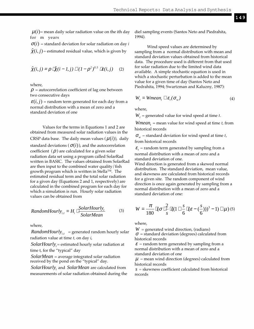
µ(i)= mean daily solar radiation value on the ith dayfor m years

σ(i) = standard deviation for solar radiation on day i

χ̂(i, j) = estimated residual value, which is given by

χ̂(i, j) = ρ ⋅ χ̂(i − 1, j) + (1 − ρ 2 )0.5 ⋅ ε(i, j)

where,ρ = autocorrelation coefficient of lag one betweentwo consecutive days

ε(i, j) = random term generated for each day from anormal distribution with a mean of zero and astandard deviation of one

Values for the terms in Equations 1 and 2 areobtained from measured solar radiation values in the

CRSP data base. The daily mean values ( µ(i)), daily

standard deviations ( σ(i) ), and the autocorrelationcoefficient ( ρ ) are calculated for a given solarradiation data set using a program called SolarRadwritten in BASIC. The values obtained from SolarRadare then input to the combined water quality/fishgrowth program which is written in Stella™. Theestimated residual term and the total solar radiationfor a given day (Equations 2 and 1, respectively) arecalculated in the combined program for each day forwhich a simulation is run. Hourly solar radiationvalues can be obtained from

RandomHourlyi,t = Hi ⋅ SolarHourlyt

SolarMean

where,

RandomHourlyi,t = generated random hourly solarradiation value at time t, on day i,

SolarHourlyt = estimated hourly solar radiation attime t, for the “typical” daySolarMean = average integrated solar radiationreceived by the pond on the “typical” day.

SolarHourlyt and SolarMean are calculated frommeasurements of solar radiation obtained during the

diel sampling events (Santos Neto and Piedrahita,1994).

Wind speed values are determined bysampling from a normal distribution with mean andstandard deviation values obtained from historicaldata. The procedure used is different from that usedfor solar radiation due to the limited wind dataavailable. A simple stochastic equation is used inwhich a stochastic perturbation is added to the meanvalue for a given time of day (Santos Neto andPiedrahita, 1994; Swartzman and Kaluzny, 1987):

Wt = Wmeant + ε t (σw )

where,

Wt = generated value for wind speed at time t.

Wmeant = mean value for wind speed at time t, fromhistorical records

σw = standard deviation for wind speed at time t,from historical records

ε t = random term generated by sampling from anormal distribution with a mean of zero and astandard deviation of one.Wind direction is generated from a skewed normaldistribution. The standard deviation, mean value,and skewness are calculated from historical recordsfor a given site. The random component of winddirection is once again generated by sampling from anormal distribution with a mean of zero and astandard deviation of one:

W = π180

⋅ (σ ⋅ 2

s⋅ ((1 + s

6⋅ (ε − (

s

6)))3 − 1) + µ )

where,W = generated wind direction, (radians)σ = standard deviation (degrees) calculated fromhistorical recordsε = random term generated by sampling from anormal distribution with a mean of zero and astandard deviation of oneµ = mean wind direction (degrees) calculated fromhistorical recordss = skewness coefficient calculated from historicalrecords

(2)

(3)

(4)

(5)

150


where,CCHL = ratio of phytoplankton carbon to

chlorophyll a, mgC

mgChla

α = slope of photosynthesis rate to light intensity (P-

I) curve, mgC

mgChla ⋅ w

m2

Imax = maximum light intensity, w

m2

µmax = maximum phytoplankton growth rate,

mgO2

mgC ⋅ hr

g(t) = temperature dependence, 1.08(t-20)

e = constant, 2.718In the model, α and µmax are inferred from a previousdeterministic model (Culberson, 1993). CCHL isdepended on the maximum light intensity Imax andwater temperature. In the present model, Imax isdetermined as the weighted average of the lightintensity for the previous three days (Lee et al. 1991b):

Imax = 0.7 Imax 1 + 0.2 Imax 2 + 0.1Imax 3

where Imax, Imax2, and Imax3 are the lightest intensitiesone, two, and three days prior to the current day

Fish growth rate

The fish growth model was adapted from themodel developed by the OSU-DAST (Bolte et al.,1994). The adaptation was carried out as part of workcarried out by the UC Davis DAST, on modeling ofintegrated aquaculture-agriculture systems, and isdescribed by Jamu and Piedrahita (Aquaculture PondModeling for the Analysis of Integrated Aquaculture/Agriculture Systems, Work Plan 8, Study 2 in thisvolume).

Temperature model

Water temperature is calculated from anenergy balance as described by Losordo (1988) and byCulberson (1993). The main heat sources in a pondare solar irradiance and atmospheric radiation.Incident solar irradiance is obtained from generatedsolar radiation values as described above.Atmospheric radiation is determined by airtemperature. The attenuation of solar irradiance withdepth in the water column is estimated by using abulk light extinction coefficient determined as afunction of Secchi disk depth. Since the daily Secchidisk depth was not available in the CRSP data base, asite-specific regression equation between Secchi diskand chlorophyll-a concentration is used in the model.Energy exchange between layers in the pond watercolumn is due to diffusion and convection (Losordo,1988). Diffusion is estimated primarily as a functionof wind speed, wind direction, and fetch (Losordo,1988; Culberson, 1993).

Dissolved Oxygen model

Dissolved oxygen concentrations aredetermined from mass balance calculations in whichphotosynthesis constitutes the main source of oxygen.Oxygen sinks include respiration by phytoplankton,fish, benthic organisms, etc. Oxygen transfer with theatmosphere may constitute a source or a sink,depending on whether the oxygen concentration inthe surface layer of the pond is below or abovesaturation. Calculation of oxygen production andconsumption rates requires some estimate ofphytoplankton concentration. In previous modelsLosordo (1988) and Culberson (1994) used measuredchlorophyll-a values, but those are not available on adaily basis as needed for simulations covering manyconsecutive days. Therefore, Culberson’s model wasmodified by adding a mass balance term forchlorophyll-a, and introducing a term relatingphytoplankton carbon to chlorophyll-a concentration(carbon:chlorophyll-a ratio, or CCHL). CCHL ishighly variable, and values are reported between 10and 1000 (Steele, 1962). An estimate of CCHL can beobtained from (Lee et al., 1991 a, b):

CCHL = 24 ⋅ α ⋅ Imax

µmaxg(t)e(6)

(7)

151


Results and Discussion

A period of 83 days was simulated, from Julianday 40 to 123, with a time step of 0.0625 hours. Thelength of the simulation was limited by the internalstructure of the modeling software (16 bit addresses,or a maximum of 32,768 steps), and was independentof hardware (same limitation on Macintosh™ andWindows™ machines). Simulation results(maximum, minimum, and average values) areobtained after running the model 50 times usingstochastically generated weather parameters asdescribed above, and are shown in Figures 1 through15. The data used for model execution were collectedat the CRSP site in Thailand, and correspond to thedata set used in the development of previous modelsby the UC Davis DAST (Santos Neto and Piedrahita,1994; Culberson , 1993). Simulated watertemperatures of the three layers are shown in Figures1 through 3. Measured values available for the 83 daytime period lie within the range of temperaturesdefined in the simulations with two exceptions, oneon day 82, and one on day 110 (0.5, and 0.3 ˚C higherthan the maximum temperatures simulated for thecorresponding times). Simulation results for themiddle and bottom layers lie further from the meanvalues, and stray beyond the range of temperaturesestimated from the simulations for the bottomtemperature for days 40 and 110 (Figures 5 and 6).

Dissolved oxygen fluctuations were morepronounced for the surface layer than for the middleand bottom layers (Figures 7-9). The probability ofthe pond dissolved oxygen concentration droppingbelow 2 mg/L was most evident during the secondhalf of the simulation period, where the minimumDO calculated often was under 2 mg/L during atleast part of the day in all three layers (Figures 7-9).The minimum DO calculated over the 50 simulationruns reached 0 mg/L for all three layers on days 102

and 103 (Figures 7-9). Comparing the simulated andmeasured DO values for the three layers shows betteragreement for the surface and middle layer than forthe bottom layer (Figures 10-12). The largefluctuations of temperature and DO are causedprimarily by the large changes of the stochasticallygenerated solar radiation values (Figure 13). Themaximum solar radiation intensity generated, I

maxranged from 500 to 2800 µmol/m2/s, with the

measured values being lower than the mean of thepredictions for most days (Figure 13).

Chlorophyll-a concentration rises throughoutthe simulation period (Figure 14), but no data areavailable in this particular data set to compare to thesimulated values. However, chlorophyll-aconcentrations are often observed to rise during agrowing season. Fish biomass is being overestimatedin the current version of the model (Figure 15), andrevisions to the fish growth estimation as a functionof feed quantity and quality, and of water qualityparameters will be necessary to improve the accuracyof the predictions.

Anticipated Benefits

The results presented in this report are for thefirst version of a model of water quality and fishgrowth in fish ponds using stochastic weather inputs.The results show the power and usefulness of using astochastic approach to simulate pond production. Bybeing able to generate a range of possible waterquality and fish yield outcomes for a site and for aparticular pond management strategy, the modelerwill be able to identify risks associated with a givenoperation and make more informed decisions on siteselection and on pond management. Improvementsare needed in the model, especially in the dissolvedoxygen and fish growth simulations.

152


Figu

re 1

. T

empe

ratu

re p

red

icti

ons

for

the

surf

ace

laye

r of

a s

trat

ifie

d p

ond

aft

er 5

0 ru

ns, a

nd o

ver

an 8

3 d

ay s

imul

atio

n. T

he m

axim

um,

min

imum

, and

mea

n te

mpe

ratu

re o

btai

ned

at e

ach

hour

of t

he s

imul

atio

n ar

e sh

own.

153


Figu

re 2

. T

empe

ratu

re p

red

icti

ons

for

the

mid

dle

laye

r of

a s

trat

ifie

d p

ond

aft

er 5

0 ru

ns, a

nd o

ver

an 8

3 d

ay s

imul

atio

n. T

he m

axim

um,

min

imum

, and

mea

n te

mpe

ratu

re o

btai

ned

at e

ach

hour

of t

he s

imul

atio

n ar

e sh

own.

154


Figu

re 3

. T

empe

ratu

re p

red

icti

ons

for

the

bott

om la

yer

of a

str

atif

ied

pon

d a

fter

50

runs

, and

ove

r an

83

day

sim

ulat

ion.

The

max

imum

,m

inim

um, a

nd m

ean

tem

pera

ture

obt

aine

d a

t eac

h ho

ur o

f the

sim

ulat

ion

are

show

n.

155


Figu

re 4

. C

ompa

riso

n of

mea

sure

d a

nd p

red

icte

d te

mpe

ratu

res

for

the

surf

ace

laye

r. T

he d

ays

show

n ar

e th

ose

for

whi

ch m

easu

red

val

ues

wer

eav

aila

ble.

156


Figu

re 5

. C

ompa

riso

n of

mea

sure

d a

nd p

red

icte

d te

mpe

ratu

res

for

the

mid

dle

laye

r. T

he d

ays

show

n ar

e th

ose

for

whi

ch m

easu

red

val

ues

wer

eav

aila

ble.

157


Figu

re 6

. C

ompa

riso

n of

mea

sure

d a

nd p

red

icte

d te

mpe

ratu

res

for

the

bott

om la

yer.

The

day

s sh

own

are

thos

e fo

r w

hich

mea

sure

d v

alue

s w

ere

avai

labl

e.

158


Figu

re 7

. D

isso

lved

oxy

gen

pred

icti

ons

for

the

surf

ace

laye

r of

a s

trat

ifie

d p

ond

aft

er 5

0 ru

ns, a

nd o

ver

an 8

3 d

ay s

imul

atio

n. T

he m

axim

um,

min

imum

, and

mea

n D

O o

btai

ned

at e

ach

hour

of t

he s

imul

atio

n ar

e sh

own.

159


Figu

re 8

. D

isso

lved

oxy

gen

pred

icti

ons

for

the

mid

dle

laye

r of

a s

trat

ifie

d p

ond

aft

er 5

0 ru

ns, a

nd o

ver

an 8

3 d

ay s

imul

atio

n. T

he m

axim

um,

min

imum

, and

mea

n D

O o

btai

ned

at e

ach

hour

of t

he s

imul

atio

n ar

e sh

own.

160


Figu

re 9

. D

isso

lved

oxy

gen

pred

icti

ons

for

the

bott

om la

yer

of a

str

atif

ied

pon

d a

fter

50

runs

, and

ove

r an

83

day

sim

ulat

ion.

The

max

imum

,m

inim

um, a

nd m

ean

DO

obt

aine

d a

t eac

h ho

ur o

f the

sim

ulat

ion

are

show

n.

161


Figu

re 1

0. C

ompa

riso

n of

mea

sure

d a

nd p

red

icte

d D

O fo

r th

e su

rfac

e la

yer.

The

day

s sh

own

are

thos

e fo

r w

hich

mea

sure

d v

alue

s w

ere

avai

labl

e.

162


Figu

re 1

1. C

ompa

riso

n of

mea

sure

d a

nd p

red

icte

d D

O fo

r th

e m

idd

le la

yer.

The

day

s sh

own

are

thos

e fo

r w

hich

mea

sure

d v

alue

s w

ere

avai

labl

e.

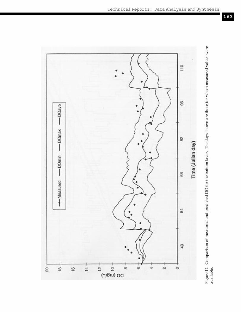
163


Figu

re 1

2. C

ompa

riso

n of

mea

sure

d a

nd p

red

icte

d D

O fo

r th

e bo

ttom

laye

r. T

he d

ays

show

n ar

e th

ose

for

whi

ch m

easu

red

val

ues

wer

eav

aila

ble.

164


Figu

re 1

3. M

axim

um s

olar

rad

iati

on in

tens

ity

(Im

ax) o

btai

ned

aft

er 5

0 si

mul

atio

ns c

ompa

red

to m

easu

red

val

ues

avai

labl

e.

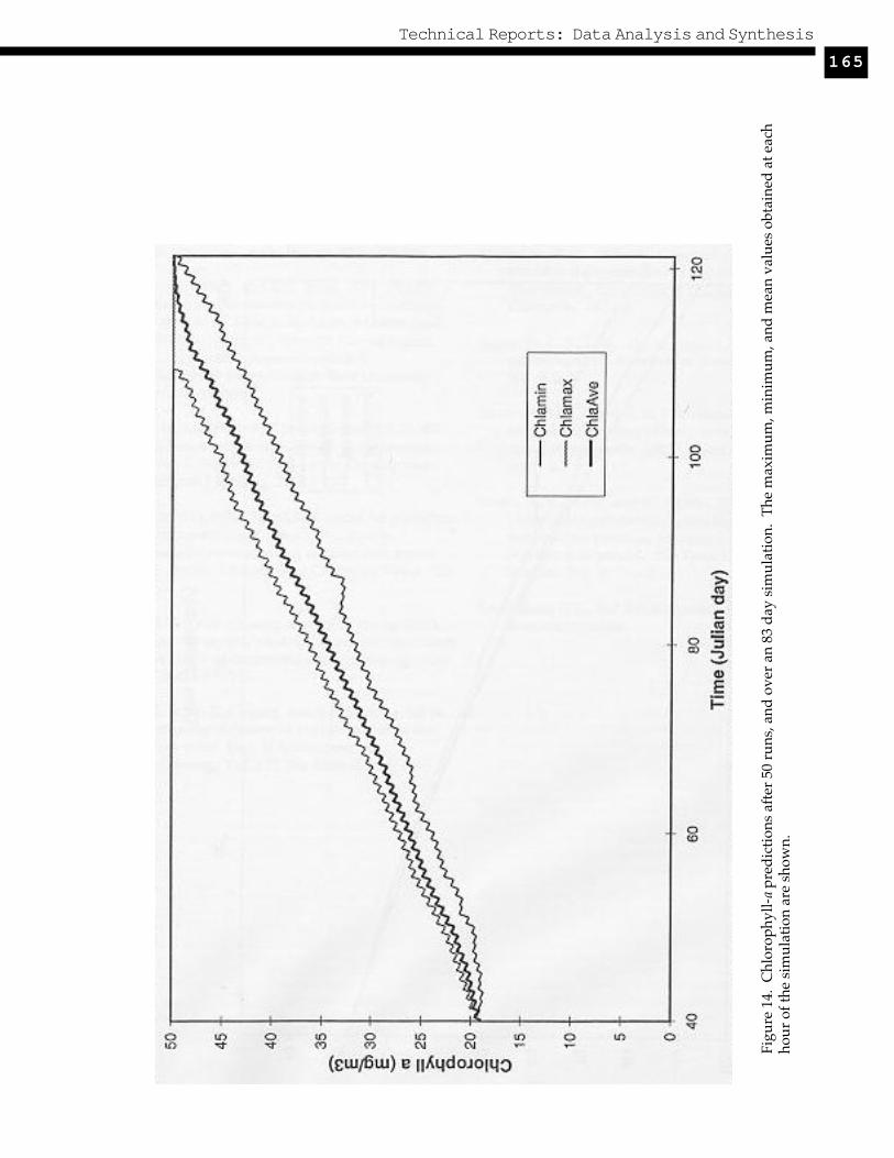
165


Figu

re 1

4. C

hlor

ophy

ll-a

pred

icti

ons

afte

r 50

run

s, a

nd o

ver

an 8

3 d

ay s

imul

atio

n. T

he m

axim

um, m

inim

um, a

nd m

ean

valu

es o

btai

ned

at e

ach

hour

of t

he s

imul

atio

n ar

e sh

own.

166


Figu

re 1

5. I

ndiv

idua

l fis

h m

ass

pred

icte

d a

fter

50

runs

com

pare

d to

mea

sure

d v

alue

s av

aila

ble.

167


Literature Cited

Amato, U. , A. Andretta, B. Bartoli, B. Coluzzi and V.Cuomo. 1986 Markov processes and fourieranalysis as a tool to describe and simulate dailysolar irradiance. Solar Energy 37(3): 179-194.

Bolte, J.P., S.S. Nath, and D.E. Ernst. 1994. POND: adecision support system for pond aquaculture.pp 48-67 In H. Egna, J. Bowman, B Goetze, andN. Weidner (Editors), Twelfth Annual Report.Pond Dynamics/Aquaculture CRSPManagement Office, Oregon State University,Corvallis, Oregon.

Cuenco, M. L., Robert R. S. and William E. G., 1985.Fish Bioenergetics and Growth in AquaculturePonds: I. Individual Fish Model DevelopmentEcological Modeling, 27:169-190.

Culberson, S.D. 1993. Simplified model for predictionof temperature and dissolved oxygen inaquaculture ponds: using reduced data inputs.M.S. Thesis. University of California, Davis. 212pp.

Lee, J. H. W., Y. K. Cheung, and P.P.S. Wong, 1991a.Dissolved oxygen variation in marine fish culturezone. Jour. of Environmental Engineering. Vol.117, No. 6:799-815.

Lee, J. H. W., Y. K. Cheung, and P.P. S. Wong, 1991b.Forecasting of dissolved oxygen in marine fishculture zone. Jour. of Environmental

Engineering. Vol. 117, No. 6:816-833.Losordo, T.M. 1988. The characterization and

modeling of thermal and oxygen stratification inaquaculture ponds. Ph.D. dissertation.University of California, Davis. 416 pp.

Piedrahita, R. H. 1984. Development of a computermodel of the aquaculture pond ecosystem. Ph.Ddissertation. University of California, Davis,California. 162 pp.

Reynolds, C. S., 1984. The ecology of freshwaterphytoplankton. Cambridge University Press.384 pp.

Santos Neto, C.D. and R.H. Piedrahita. 1994.Stochastic modeling of temperature in stratifiedaquaculture ponds. CRSP report, work plan 7,study 2.

Sedeh, A., C. Pardy and W. Griffin, 1986.Uncertainty consideration resulting fromtemperature variation on growth of PenaeusStylirostris in ponds., The Texas Journal ofScience., Vol. 38. No. 2.

Swartzman, G.L., and S.P. Kaluzny. 1987. Ecologicalsimulation primer.

Stochastic Modeling of Temperature and Dissolved Oxygen in...

Documents

Transcript of Stochastic Modeling of Temperature and Dissolved Oxygen in...