Stochastic Modeling of Advection-Di usion-Reaction...
164
UNIVERSITY OF CALIFORNIA, SAN DIEGO Stochastic Modeling of Advection-Diffusion-Reaction Processes in Biological Systems A dissertation submitted in partial satisfaction of the requirements for the degree Doctor of Philosophy in Engineering Sciences (Mechanical Engineering) by TaiJung Choi Committee in charge: Daniel M. Tartakovsky, Chair Shankar Subramaniam, Co-Chair Marcos Intaglietta Ratneshwar Lal Mano R. Maurya Sutanu Sarkar 2013
Transcript of Stochastic Modeling of Advection-Di usion-Reaction...

UNIVERSITY OF CALIFORNIA, SAN DIEGO
Stochastic Modeling of Advection-Diffusion-Reaction Processes inBiological Systems
A dissertation submitted in partial satisfaction of the
requirements for the degree
Doctor of Philosophy
in
Engineering Sciences (Mechanical Engineering)
by
TaiJung Choi
Committee in charge:
Daniel M. Tartakovsky, ChairShankar Subramaniam, Co-ChairMarcos IntagliettaRatneshwar LalMano R. MauryaSutanu Sarkar
2013

Copyright
TaiJung Choi, 2013
All rights reserved.

The dissertation of TaiJung Choi is approved, and it is
acceptable in quality and form for publication on micro-
film and electronically:
Co-Chair
Chair
University of California, San Diego
2013
iii

DEDICATION
To “my family, my advisers, my friends”.
iv

TABLE OF CONTENTS
Signature Page . . . . . . . . . . . . . . . . . . . . . . . . . . . . . . . . . . iii
Dedication . . . . . . . . . . . . . . . . . . . . . . . . . . . . . . . . . . . . . iv
Table of Contents . . . . . . . . . . . . . . . . . . . . . . . . . . . . . . . . . v
List of Figures . . . . . . . . . . . . . . . . . . . . . . . . . . . . . . . . . . viii
List of Tables . . . . . . . . . . . . . . . . . . . . . . . . . . . . . . . . . . . ix
Acknowledgements . . . . . . . . . . . . . . . . . . . . . . . . . . . . . . . . x
Vita and Publications . . . . . . . . . . . . . . . . . . . . . . . . . . . . . . xi
Abstract of the Dissertation . . . . . . . . . . . . . . . . . . . . . . . . . . . xiii
Chapter 1 Introduction . . . . . . . . . . . . . . . . . . . . . . . . . . . . 11.1 Multi-scale modeling in biology . . . . . . . . . . . . . . 11.2 Stochasticity in biology . . . . . . . . . . . . . . . . . . . 21.3 Hybrid algorithms for multi-scale systems . . . . . . . . . 4
1.3.1 Motivation . . . . . . . . . . . . . . . . . . . . . . 41.3.2 Temporal multi-scale processes . . . . . . . . . . . 51.3.3 Temporal and spatial multi-scale processes . . . . 6
1.4 Conclusions and future directions . . . . . . . . . . . . . 9
Chapter 2 Stochastic Hybrid Modeling of Intracellular Calcium Dynamics 112.1 Introduction . . . . . . . . . . . . . . . . . . . . . . . . . 112.2 Dynamics of Cytosolic Calcium . . . . . . . . . . . . . . 15
2.2.1 Biological mechanisms and pathways . . . . . . . 152.2.2 Mathematical representations of calcium dynamics 17
2.3 Materials and Methods . . . . . . . . . . . . . . . . . . . 182.3.1 The mathematical model of cytosolic calcium dy-
namics . . . . . . . . . . . . . . . . . . . . . . . . 192.3.2 Comparison of computational efficiency of stochas-
tic simulation algorithms . . . . . . . . . . . . . . 212.3.3 A multi-scale hybrid approach . . . . . . . . . . . 222.3.4 Application to cytosolic calcium dynamics in RAW
cells . . . . . . . . . . . . . . . . . . . . . . . . . 302.4 Results . . . . . . . . . . . . . . . . . . . . . . . . . . . . 31
2.4.1 Dose response . . . . . . . . . . . . . . . . . . . . 322.4.2 Convergence of stochastic simulations at low doses 33
v

2.4.3 Random variability of the [Ca2+]i response at lowdoses . . . . . . . . . . . . . . . . . . . . . . . . . 34
2.4.4 Sensitivity analysis . . . . . . . . . . . . . . . . . 352.4.5 Calcium response to protein knockdown . . . . . . 37
2.5 Summary and Discussion . . . . . . . . . . . . . . . . . . 392.5.1 Methodological novelty . . . . . . . . . . . . . . . 392.5.2 Sensitivity analysis . . . . . . . . . . . . . . . . . 402.5.3 Knockdown (KD) analysis . . . . . . . . . . . . . 422.5.4 Stochastic effects at low molecular numbers . . . 432.5.5 Deriving statistics from stochastic simulation . . . 44
Chapter 3 Stochastic Operator Splitting Approach for Reaction-DiffusionProcesses . . . . . . . . . . . . . . . . . . . . . . . . . . . . . 573.1 Introduction . . . . . . . . . . . . . . . . . . . . . . . . . 573.2 Methods: Numerical approach . . . . . . . . . . . . . . . 61
3.2.1 Operator-splitting method . . . . . . . . . . . . . 613.2.2 Algorithms for the stochastic operator-splitting
method . . . . . . . . . . . . . . . . . . . . . . . . 643.2.3 Comparison of our method with GMP method . . 69
3.3 Results: Case studies . . . . . . . . . . . . . . . . . . . . 713.3.1 Synthetic reaction-diffusion case study . . . . . . 713.3.2 Gene expression case study . . . . . . . . . . . . . 753.3.3 CheY diffusion case study . . . . . . . . . . . . . 80
3.4 Summary and Discussion . . . . . . . . . . . . . . . . . . 82
Chapter 4 Stochastic Models of Chemotaxis-Diffusion-Reaction Processesin Wound Healing . . . . . . . . . . . . . . . . . . . . . . . . 1034.1 Introduction . . . . . . . . . . . . . . . . . . . . . . . . . 1034.2 Wound healing . . . . . . . . . . . . . . . . . . . . . . . 106
4.2.1 Hemostasis . . . . . . . . . . . . . . . . . . . . . . 1064.2.2 Inflammation . . . . . . . . . . . . . . . . . . . . 1074.2.3 Proliferation . . . . . . . . . . . . . . . . . . . . . 1094.2.4 Remodeling . . . . . . . . . . . . . . . . . . . . . 110
4.3 A mathematical model of inflammation . . . . . . . . . . 1104.3.1 Diffusion . . . . . . . . . . . . . . . . . . . . . . . 1114.3.2 Chemotaxis . . . . . . . . . . . . . . . . . . . . . 1124.3.3 Reactions . . . . . . . . . . . . . . . . . . . . . . 113
4.4 Numerical approach . . . . . . . . . . . . . . . . . . . . . 1144.5 Simulation results . . . . . . . . . . . . . . . . . . . . . . 115
4.5.1 Chemotaxis and diffusion . . . . . . . . . . . . . . 1154.5.2 Chemotaxis, diffusion and reactions . . . . . . . . 118
4.6 Summary and Discussion . . . . . . . . . . . . . . . . . . 119
vi

Chapter 5 Conclusions . . . . . . . . . . . . . . . . . . . . . . . . . . . . 127
Appendix A Existing algorithms for stochastic simulation . . . . . . . . . . 131A.1 Gillespie algorithm . . . . . . . . . . . . . . . . . . . . . 134A.2 Tau-leap algorithm . . . . . . . . . . . . . . . . . . . . . 135A.3 Chemical Langevin equation . . . . . . . . . . . . . . . . 137
Appendix B Diffusion processes and GMP algorithm . . . . . . . . . . . . . 138B.1 Diffusion process: Brownian dynamics . . . . . . . . . . . 138B.2 Diffusion process: Cellular automata . . . . . . . . . . . 139B.3 Gillespie multi-particle (GMP) method . . . . . . . . . . 140
Bibliography . . . . . . . . . . . . . . . . . . . . . . . . . . . . . . . . . . . 142
vii

LIST OF FIGURES
Figure 2.1: A simplified model for calcium signaling including calcium in-flux, ER, and mitochondrial exchange and storage. . . . . . . . 49
Figure 2.2: Temporal evolution of the concentrations of substrate, S(t),and product, P (t), computed using the Gillespie, tau-leap, andchemical Langevin equation (CLE) approaches. . . . . . . . . . 50
Figure 2.3: Dose response. . . . . . . . . . . . . . . . . . . . . . . . . . . . 51Figure 2.4: Revelation of stochastic effects at low doses. . . . . . . . . . . . 52Figure 2.5: Sensitivity analysis. . . . . . . . . . . . . . . . . . . . . . . . . 53Figure 2.6: Knockdown response of PLCβ. . . . . . . . . . . . . . . . . . . 54Figure 2.7: Knockdown response of GRK. . . . . . . . . . . . . . . . . . . . 55Figure 2.8: The Ca2+
i response to the simultaneous knockdown of GRK andgene/protein related to Vmax,IP3dep. . . . . . . . . . . . . . . . . 56
Figure 3.1: Schematic representation of the diffusion-reaction operator-splitting.The final value after diffusion process at time t+ ∆t is used asthe initial value for the reaction process. . . . . . . . . . . . . . 94
Figure 3.2: Histogram of ln(1/r), where r is a uniformly distributed randomvariable in [0,1 . . . . . . . . . . . . . . . . . . . . . . . . . . . 95
Figure 3.3: Temporal evolution of the count of molecules at the center cellaveraged over 512 realizations of cellular automata (CA) andBrownian dynamics (BD). . . . . . . . . . . . . . . . . . . . . . 96
Figure 3.4: A+B → C case study: (A) Initially, species A and B exist onlyin left-hand side. All A and B molecules and their product Pdiffuse with the same diffusion constant. . . . . . . . . . . . . . 97
Figure 3.5: A+B → C case study: Effect of diffusion constant, D (m2/s),on (A) τD (or ∆t) and (B) computational time for our methodand the GMP method. . . . . . . . . . . . . . . . . . . . . . . . 98
Figure 3.6: A+B → C case study: (A)-(B) As cell size becomes finer, theresults from our approach converge to the numerical solution. . 99
Figure 3.7: Gene expression case study: (A) Dash-dotted line shows the re-sult of Gillespie algorithm which deals with only reaction process.100
Figure 3.8: Gene expression case study: (A) The result of GMP algorithmfor various L and the corresponding ∆t (= τD) values. . . . . . 101
Figure 3.9: CheY diffusion case study. . . . . . . . . . . . . . . . . . . . . . 102
Figure 4.1: Leukocytes flow along the blood stream. When injury occurs inthe tissue, they begin to roll and adhere on endothelium cells. . 123
Figure 4.2: 1D diffusion and chemotaxis. . . . . . . . . . . . . . . . . . . . 124Figure 4.3: 2D diffusion and chemotaxis. . . . . . . . . . . . . . . . . . . . 125Figure 4.4: 3D diffusion, chemotaxis and reactions. . . . . . . . . . . . . . . 126
viii

LIST OF TABLES
Table 2.1: The run-time scalability of the Gillespie, tau-leap, and chemicalLangevin equation algorithms as a function of the number ofmolecules. . . . . . . . . . . . . . . . . . . . . . . . . . . . . . . 46
Table 2.2: Criteria used to identify slow and fast reactions and correspond-ing numerical method. Column 2 and 3 list the scale and simu-lation method in the “scale (method)” format. . . . . . . . . . . 47
Table 2.3: Summary of results of KD response. The change in the featuresof calcium response listed is for increase in KD-level (decreasein IC:[.]) of the protein. Qualitative nature of the features ismostly independent of the level of [R]. . . . . . . . . . . . . . . . 48
Table 3.1: The tunable parameter k1 is used as a criterion to decide if thesystem is diffusion- or reaction-controlled. . . . . . . . . . . . . . 86
Table 3.2: Comparison of computational time for cellular automata andBrownian dynamics. . . . . . . . . . . . . . . . . . . . . . . . . . 87
Table 3.3: A synthetic reaction-diffusion system A+B → C with diffusionconstant D = 10−12 m2/s. . . . . . . . . . . . . . . . . . . . . . . 88
Table 3.4: Gene expression case study: DNA has 1 molecule and RNAp has18 molecules. . . . . . . . . . . . . . . . . . . . . . . . . . . . . . 89
Table 3.5: Gene expression case study: Reaction time is averaged over 256realizations of a simplified gene expression process. . . . . . . . . 90
Table 3.6: Gene expression case study. According to the central limit the-orem, noise level or standard deviation decreases as 1/
√Nr. . . . 91
Table 3.7: CheY diffusion case study: kf and kb denote respectively forwardand backward reaction rate constants for the E. coli system. . . 92
Table 3.8: CheY diffusion case study: 13 species and 13 reactions in the E.coli system. . . . . . . . . . . . . . . . . . . . . . . . . . . . . . 93
Table 4.1: Constants for reaction, diffusion and chemotaxis. . . . . . . . . . 121Table 4.2: Initial number of bacteria and leukocytes are 50 and 500. 32
simulations are conducted for 10000 sec. . . . . . . . . . . . . . . 122
ix
ACKNOWLEDGEMENTS
I would like to acknowledge Professor Daniel Tartakovsky and Shankar Sub-
ramaniam for their support as advisors during my doctoral period. I would also
like to appreciate Doctor Mano Maurya for his help and advices. Through many
research topics and multiple drafts for journal papers and dissertation, their guid-
ance has proved to be very priceless and invaluable to me.
The text of this dissertation includes the reprints of the following papers,
either accepted or submitted for consideration at the time of publication. The
dissertation author was the primary investigator and author of these publications.
Chapter 2
TaiJung Choi, Mano R. Maurya, Daniel M. Tartakovsky, Shankar Subramaniam
(2010), ‘Stochastic Hybrid Modeling of Intracellular Calcium Dynamics’. J. Chem.
Phys., 133, 165101.
Chapter 3
TaiJung Choi, Mano R. Maurya, Daniel M. Tartakovsky, Shankar Subramaniam
(2012), ‘Stochastic Operator-Splitting Method for Reaction-Diffusion Systems’. J.
Chem. Phys., 137, 184102.
Chapter 4
TaiJung Choi, Mano R. Maurya, Daniel M. Tartakovsky, Shankar Subramaniam
(2013), ‘Stochastic Modeling of Chemotaxis-Diffusion-Reaction Processes’. Under
preparation.
x

VITA
2012 Ph.D. in Mechanical and Aerospace Engineering, Universityof California, San Diego.
2004 M.S. in Mechanical and Aerospace Engineering, Seoul Na-tional University, Seoul, Korea
2002 B.S. in Mechanical Engineering, Korea University, Seoul, Ko-rea
JOURNAL PUBLICATIONS
TaiJung Choi, Mano R. Maurya, Daniel M. Tartakovsky, Shankar Subramaniam(2010), ‘Stochastic Hybrid Modeling of Intracellular Calcium Dynamics’. J. Chem.Phys., 133, 165101.
TaiJung Choi, Mano R. Maurya, Daniel M. Tartakovsky, Shankar Subramaniam(2012), ‘Stochastic Operator-Splitting Method for Reaction-Diffusion Systems’. J.Chem. Phys., 137, 184102.
TaiJung Choi, Mano R. Maurya, Daniel M. Tartakovsky, Shankar Subramaniam(2013), ‘Stochastic Modeling of Chemotaxis-Diffusion-Reaction Processes’. Underpreparation.
SELECT PRESENTATIONS
TaiJung Choi, Mano R. Maurya, Daniel M. Tartakovsky, Shankar Subramaniam,‘Stochastic Simulation of Cytosolic Calcium Dynamics’, (2009) AIChE AnnualMeeting, Nashville, TN, November 8-13.
Mano R. Maurya, TaiJung Choi, Daniel M. Tartakovsky, Shankar Subramaniam,‘Timescale Analysis of Cytosolic Calcium Dynamics’, (2010) AIChE Annual Meet-ing, Salt Lake City, UT, November 7-12.
TaiJung Choi, Mano R. Maurya, Daniel M. Tartakovsky, Shankar Subramaniam,‘Stochastic Operator Splitting Method for Biological Systems’, (2011) AIChE An-nual Meeting, Minneapolis, MN, October 16-21.
POSTER PRESENTATIONS
xi
TaiJung Choi, Mano R. Maurya, Daniel M. Tartakovsky, Shankar Subramaniam,‘Stochastic Modeling of Calcium Dynamics in RAW 264.7 Cells’, (2010) ResearchExpo, University of California, San Diego, April 15.
TaiJung Choi, Mano R. Maurya, Daniel M. Tartakovsky, Shankar Subramaniam,
‘Stochastic Operator-Splitting Method for Reaction-Diffusion Process’, (2011) Re-
search Expo, University of California, San Diego, April 14.
xii

ABSTRACT OF THE DISSERTATION
Stochastic Modeling of Advection-Diffusion-Reaction Processes inBiological Systems
by
TaiJung Choi
Doctor of Philosophy in Engineering Sciences (Mechanical Engineering)
University of California, San Diego, 2013
Daniel M. Tartakovsky, ChairShankar Subramaniam, Co-Chair
This dissertation deals with complex and multi-scale biological processes.
In general, these phenomena can be described by ordinary or partial differential
equations and treated with deterministic methods such as Runge-Kutta and al-
ternating direction implicit algorithms. However, these approaches cannot predict
the random effects caused by the low number of molecules involved and can re-
sult in severe stability and accuracy problem due to wide range of time or length
scales depending upon the system being studied. In the first part of the disserta-
tion, therefore, we develope the stochastic hybrid algorithm for complex reaction
networks. Deterministic models of biochemical processes at the subcellular level
might become inadequate when a cascade of chemical reactions is induced by a few
xiii
molecules. Inherent randomness of such phenomena calls for the use of stochastic
simulations. However, being computationally intensive, such simulations become
infeasible for large and complex reaction networks. To improve their computa-
tional efficiency in handling these networks, we present a hybrid approach, in
which slow reactions and fluxes are handled through exact stochastic simulation
and their fast counterparts are treated partially deterministically through chemical
Langevin equation. The classification of reactions as fast or slow is accompanied
by the assumption that in the time-scale of fast reactions, slow reactions do not
occur and hence do not affect the probability of the state. In the second and third
part of the dissertation, we employ stochastic operator splitting algorithm for
(chemotaxis-)diffusion-reaction processes. The reaction and diffusion steps employ
stochastic simulation algorithm and Brownian dynamics, respectively. Through
theoretical analysis, we develop an algorithm to identify if the system is reaction-
controlled, diffusion-controlled or is in an intermediate regime. The time-step size
is chosen accordingly at each step of the simulation. We apply our algorithm to
several examples in order to demonstrate the accuracy, efficiency and robustness
of the proposed algorithm comparing with the solutions obtained from determin-
istic partial differential equations and Gillespie multi-particle method. The third
part deals with application of the stochastic-operator splitting approach to model
the chemotaxis of leukocytes as part of the inflammation process during wound
healing. We analyze both chemotaxis as well as the diffusion process as a drift
phenomenon. We use two dimensionless numbers, Damkohler and Peclet num-
xiv

ber, in order to analyze the system. Damkohler number determines if the system
is reaction-controlled or drift controlled and Peclet number identifies which phe-
nomenon is dominant between diffusion and chemotaxis.
xv

Chapter 1
Introduction
1.1 Multi-scale modeling in biology
Biological systems involve various processes taking place at a wide range
of spatial and temporal scales. Biological systems have spatial scales which range
from kilometers, e.g. the habitat of animals, to micrometers such as phenomena at
the cellular level. The spatial scales can range from meters to microns in dealing
with a single organism. Within the intercellular space, depending upon the context,
the spatial domain of interest can vary from nanometers to micrometers. Similar
phenomena is observed for the temporal scale. For example, population fluctuation
of some animal group can be detected at the time scale of years whereas events
such as cell division occur on a scale of hours and molecular chemical reactions
take place within milliseconds to minutes. Specially at subcellular volumes when
the number of molecules can be low so that the continuum approximation becomes
1
2
invalid, stochastic effects become important. The interplay of stochasticity with
the multiplicity in the spatial and temporal domains is complex. Not accounting
the different time and spatial scales in the modeling and simulation of stochastic
systems results in errors and/or large simulation times. The development of robust
mathematical techniques for the modeling and simulation of stochastic biological
systems with multiscale temporal and spatial scales is the main focus of this dis-
sertation. The stochasticity is quantitatively modeled through the use of random
variables. In addition, this dissertation also deals with approaches to account for
multiple spatial and temporal scales. In this dissertation, several biological sys-
tems are used to demonstrate the effectiveness of methodologies developed. The
biological systems include (1) regulation of the dynamics of intracellular calcium
ion levels, (2) molecular diffusion and reactions in E coli and (3) leukocyte chemo-
taxis through the tissue during the inflammation phase of wound healing process.
These case studies are linked with each other in various ways and at various bio-
logical scales (from intracellular to tissue level) and serve as excellent test-beds in
multi-scale mathematical modeling and quantitative systems biology.
1.2 Stochasticity in biology
Over the last few decades, in the field of molecular biology, the importance
of stochasticity has been increasingly recognized and outstanding developments
have led to a better understanding of biological systems at the subcellular level.
3
At the level of micro-scale systems such as the interactions between molecules, e.g.
DNA, mRNA, protein, small molecules, it follow an important law of physics, i.e.,
randomness or fluctuations in a system are inversely proportional to the square
root of the number of particles [1]. Therefore, a lower number of molecules (or low
concentration) results in high fluctuation which is largely due to thermal oscilla-
tions. For example, in processes such as gene transcription/regulation and signal
transduction [2], number of molecules involved in the chemical reactions is usually
low, e.g., a single DNA template, tens of mRNA molecules and around hundred
molecules of transcription factors. Such stochastic effects arising due to the in-
herent nature of biochemical interactions are often termed as intrinsic noise. In
addition, there exists an extrinsic noise as well caused by random fluctuations in
other factors such as the number of ribosomes, the stage of the cell cycle, mRNA
degradation, and the cellular environment [3]. Yarchuk et al. showed that protein
production occurs in short bursts at random time intervals rather than in a contin-
uous manner [4]. In addition, spatial randomness plays an important role during
processes such as E. coli movement [5], tumor growth [6] and leukocyte chemotaxis
[7].

4
1.3 Hybrid algorithms for multi-scale systems
1.3.1 Motivation
Intracellular signaling is an important event in cellular life that mediates
most of cell functions, such as adaptation in response to environmental changes,
metabolism, cellular growth and proliferation. Mathematical modeling, tradition-
ally based on ordinary differential equations, helped to explain and illustrate many
of these complex phenomena, including the bistability and graded versus switch-
like response in intracellular signaling [8] and sub-population variability [9]. ODE-
based formulations offer accurate predictions of biochemical dynamics with large
numbers of molecules, but are expected to fail if the numbers of reacting molecules
become exceedingly small. When this occurs, randomness associated with the
dynamics of individual molecules becomes important and calls for a probabilistic
(stochastic) description. Chapter 2 provides an example of such modeling in the
context of intracellular calcium dynamics.
All ODE-based models, and most of stochastic models of the type dis-
cussed above, are based on the assumption of a perfectly mixed (homogeneous)
system, in which every point (or volume) in space has the same concentration
(or number of molecules) of reacting species. This assumption becomes invalid
when the number of reacting molecules becomes small and transport also take
place in heterogeneous crowded environments. In Chapters 3 and 4, we develop
computational methods to deal with such spatial heterogeneity in the context of

5
molecular diffusion and reactions in E. coli (Chapter 3) and leukocyte chemo-
taxis (Chapter 4). These two biological phenomena illustrate the complexity of
most cellular processes by exhibiting multiple time and length scales, randomness
and spatial inhomogeneity. These chapters present a new stochastic hybrid algo-
rithm for multi-scale systems and a new stochastic operator splitting algorithm for
(chemotaxis-)diffusion-reaction systems, respectively.
1.3.2 Temporal multi-scale processes
In Chapter 2, we present a novel algorithm for the stochastic simulation
of multi-scale (time-domain) biochemical processes. The methodology is applied
to study intracellular calcium dynamics in mouse RAW 264.7 macrophage cells.
Intracellular signaling plays an important role in cellular life that regulates most of
its functions, such as adaptation in response to environmental changes and regular
functions including metabolism, cellular growth and proliferation. Mass balance
for chemical reactions which is described by ordinary differential equations (ODE)
is generally applied to analyze these chemical reactions. These ODE-based for-
mulations can predict accurately the dynamics of biochemical pathways with large
numbers of molecules of all reacting species. However, it might fail in the case that
the concentrations of involved chemical species become exceedingly small [10]. In
this case, it is necessary to apply stochastic analysis which treat chemical reactions
as random events. A chemical master equation (CME) yields an exact probabilistic
description of multi-species reactions, but its high dimensionality renders it com-

6
putationally prohibitive. Gillespie algorithm [11], a good approximation of CMEs,
deals with all possible reactions using uniformly distributed random variables in
[0,1]. A tau-leap algorithm [12] or chemical Langevin equation (CLE) [13] can
further approximate CME using Poisson random variables and Gaussian random
variables, respectively. Implicit in these and other approximations of the SSA is a
trade-off between computational speed-up and accuracy, which undermines their
use in complex multi-scale biochemical phenomena involving fast and slow reac-
tions. Therefore, we present a hybrid algorithm in which slow and fast reactions
are identified, they can be reclassified during simulation in response to changes
in concentrations, and we can deal with complex fluxes that cannot be modeled
explicitly through reactions.
1.3.3 Temporal and spatial multi-scale processes
In Chapters 3 and 4, we investigate diffusion-reaction systems in various
biological systems such as CheY diffusion in E. coli (Chapter 3) and inflammation
process during wound healing (Chapter 4). In addition to randomness from small
number of molecules, we have stochasticity due to inhomogeneity of molecules
across the space. In order to simulate the spatial variation, mesh/grid-based ap-
proaches are used. The number of molecules within each voxel can be low resulting
in stochasticity. Therefore, we have to deal with two types of randomness, i.e., in
the temporal domain and in the spatial domain. Partial differential equations
(PDEs) can predict accurately the dynamics of spatially heterogeneous systems

7
composed of chemical species with high concentration. However, similar to ODE-
based models, they fail to account for the randomness inherent in a system com-
prised of small number of molecules. A number of simulation methods have been
developed for the simulation of reaction-diffusion systems. The Green’s function
reaction dynamics [14] and Smoldyn’s algorithm [15], employs Brownian dynam-
ics to track the diffusion of molecules and assume that bimolecular reactions can
take place when two molecules exist within a certain distance. These requirements
necessitate the tracking of individual particles and/or distances between them,
which makes such algorithms computationally expensive. MesoRD [16] and the
Gillespie multi-particle (GMP) methods [17, 18] trade representational accuracy
for computational efficiency. They are based on a reaction-diffusion master equa-
tion [19], which generalizes a chemical master equation developed for well-mixed
chemical reactions by discretizing the space into a collection of cells and treating
each cell as a well mixed system. MesoRD [16] treats diffusion as a unimolecular
reaction whose reaction rate is related to the corresponding diffusion coefficient.
The GMP method [17, 18] employs an operator-splitting scheme in which the Gille-
spie algorithm and cellular automata [20] handle reaction and diffusion processes,
respectively.
We have developed a stochastic numerical algorithm to simulate reaction-
diffusion processes with a small number of non-uniformly distributed molecules. It
employs an operator-splitting, in which the Gillespie algorithm [11] and Brownian
dynamics are used to simulate reaction and diffusion processes, respectively. Our
8
algorithm is conceptually similar to the GMP method in that it relies on operator-
splitting. However, it offers a number of computational advantages in terms of both
accuracy and efficiency. First, the cellular automata used in the GMP method re-
strict a particle’s movement during one fixed time-step to the adjacent cells only,
while Brownian motion places no restrictions on the distance particles can travel
during one time-step, thus gaining in computational efficiency. Second, Brown-
ian dynamics provides a more accurate representation of diffusion than cellular
automata. Third, our algorithm offers the flexibility of adaptive selection of the
time-step sizes for operator-splitting, depending on whether the system is reaction-
or diffusion-controlled.
We have also studied the inflammation process during wound healing in
which leukocyte cells sense the gradient of chemoattractants from the wound site
and chemotax in the direction of higher concentration while also diffusing ran-
domly. It involves three processes, diffusion, reaction and chemotaxis. In addition
to the diffusion-reaction processes explained above, we also have to deal with the
chemotaxis process. In order to identify the drift (chemotaxis + diffusion) time
scale, Peclet number is introduced. Damkohler number decides if system is diffu-
sion or reaction controlled.
9
1.4 Conclusions and future directions
In biological systems, randomness is caused by small number of molecules
and spatial inhomogeneity. Therefore, we have developed stochastic hybrid algo-
rithms for multi-scale reaction systems, in which chemical reactions are classified
as fast or slow according to propensity functions and chemical species are clas-
sified as low or high based on the number of molecules. We applied our hybrid
algorithm to intracellular calcium dynamics in mouse macrophage cells by apply-
ing Gillespie algorithm or Chemical Langevin equation appropriately according
to system’s state. Next, we have developed stochastic operator-splitting method
for (chemotaxis)-diffusion-reaction systems. Proper selection of time step is very
important because drift (chemotaxis, diffusion) time constant and reaction time
constant may be significantly different. Furthermore, one needs to identify the
dominant process between diffusion and chemotaxis. Hence, we use Damkohler
and Peclet numbers. In this dissertation, these novel methodologies have been
developed and applied to interesting biological systems in order to verify accu-
racy, efficiency and robustness of the proposed algorithms. We have applied these
approaches to several biological systems of low to moderate complexity.
In the future, these approaches can be tested on more complex and realis-
tic systems. For example, stem cells exist during all phases of development, e.g.,
embryonic stem (ES) cells during the embryonic stage and adult stem cells after
all the organs are formed. Stem cells are characterized by two important abilities,

10
viz., renew themselves and differentiate into a variety of distinct lineages. ES cells
are omnipotent or pluripotent i.e., they have the ability to generate all embryonic
tissues. Due to their potential to regenerate tissue damaged due to disease or in-
jury, stem cell-based therapies for various degenerative diseases are being developed
[?]. Stem cell properties are governed by a complex set of interactions between
signaling from the extracellular and intercellular environment and the dynamics
of core transcriptional machinery. Spatial variability plays an important role in
this process. Therefore, we can apply our operator-splitting approach to stochas-
tic stem-cell fate decision modeling in order to quantitatively study the molecular
mechanism of ES cells [?]. In another application, we will consider all processes
from rolling to chemotaxis of leukocytes based on our stochastic operator-splitting
method because spatial variation is important for the leukocyte movement inside
the capillary, across endothelial cell wall and through the tissue. We will employ
different boundary and initial conditions for these three connected spatial zones.
We will perform a comprehensive quantitative analysis of leukocyte motion during
wound healing process by accounting for blood flow, wall shear stress and contact
force between endothelial cells.
Chapter 2
Stochastic Hybrid Modeling of
Intracellular Calcium Dynamics
2.1 Introduction
Intracellular signaling is an important event in cellular life that mediates
most of its functions, such as adaptation in response to environmental changes and
regular functions including metabolism, cellular growth and proliferation. Math-
ematical modeling has helped to explain and illustrate many of these complex
phenomena, including the bistability and graded versus switch-like response in in-
tracellular signaling [8], auto-catalysis as a mechanism of positive feedback in the
cell cycle [21], and sub-population variability [9]. Much of this modeling is done in
a deterministic setting, and involves systems of coupled ordinary differential equa-
tions (ODEs) describing the rate of change of components (reactants and products)
11

12
of the biochemical reactions and other processes involved in the pathway.
ODE-based formulations provide accurate predictions of the dynamics of
biochemical pathways with large numbers of molecules of all reacting species, but
might fail when the concentrations of reactants and/or products become exceed-
ingly small so than only a few molecules (less than 10 in some cases) are involved
[10]. Indeed, for small volumes and small concentrations that often characterize
sub-cellular processes, the very concept of concentration breaks down. When this
occurs, randomness associated with the dynamics of individual molecules becomes
pronounced, necessitating the use of probabilistic (stochastic) models. A chemical
master equation (CME) yields an exact probabilistic description of multi-species
reactions, but its high dimensionality renders it computationally prohibitive.
Gillespie’s stochastic simulation algorithm (SSA) [11] provides an exact
sampling of the solution of the CME, thus providing highly accurate results with
sufficient sampling. The computational efficiency of the SSA can be increased by
adopting, for example, a tau-leap algorithm [12] or its continuous-limit approxi-
mation in the form of a chemical Langevin equation (CLE) [13]. Implicit in these
and other approximations of the SSA is a trade-off between computational speed-
up and accuracy, which undermines their use in complex multi-scale biochemical
phenomena involving fast and slow reactions. A quasi-steady-state approximation
[22], which neglects the fast reactions by assuming that a subset of chemical species
is at steady state at the timescale of interest, is efficient but clearly inexact.
Some of the more recent contributions in this area include: (1) speed-up of

13
computation through a binomial tau-leaping approach [23] and k-skip method [24],
(2) time-scale/reaction partitioning based on the propensity values [25], a hybrid
approach [26] and quasi-steady-state approximation [27], (3) partial-propensity-
based approach [28] and (4) alternative formulations of CLE [29]. Besides, [30] has
developed an approach to perform stochastic simulation of reaction systems with
time-delays. [31] have developed a software called Biomolecular Network Simulator
to study various aspects of stochastic simulation of complex biomolecular reaction
networks. [32] have presented a detailed analysis of issues in simplification of
Michaelis-Menten formulation into a single-step reaction in stochastic simulation.
[33] have developed a methodology for parametric sensitivity analysis in stochastic
simulation of reaction networks. By no means this is an exhaustive list.
Hybrid methods, e.g., by [26], which we pursue here, address the multi-scale
nature of reactive systems by identifying fast and slow reactions, and simulating the
former with a CLE and the latter with Gillespie’s SSA. This approach significantly
reduces simulation time without compromising the accuracy of the outputs. We
present a hybrid algorithm in which slow and fast reactions are identified a priori,
they can be reclassified during simulation in response to changes in concentrations,
and we can deal with complex fluxes that cannot be modeled explicitly through
reactions. An example of such as flux, in the model of cytosolic calcium dynamics,
is the flux of [Ca2+] from the endoplasmic reticulum to the cytosol through inositol
1,4,5- trisphosphate receptor channels (please see the expression for Jch in Section
2.3.3).

14
We have used the dynamics of cytosolic calcium as a case study to test
our approach. The cytosolic calcium dynamics and its mathematical descriptions
are briefly discussed in Section 3.2 to motivate the development of a multi-scale
stochastic hybrid algorithm (SHA) in section 2.3, which consists of the following
steps. Section 2.3.1 contains a formulation of the calcium dynamics model used in
our analysis. In Section 2.3.2, we compare the performance of existing stochastic
approaches, i.e., the Gillespie’s SSA, a tau-leap algorithm, and a chemical Langevin
equation. In Section 2.3.3, we present the SHA, which consists of deterministic
and stochastic components, explicitly accounts for the presence of slow and fast
reactions, and incorporates complex fluxes that cannot be modeled through reac-
tions explicitly. An approach to handle reactions with complex rate expressions
is also presented in this section explaining why the existing approaches to deal
with complex rates laws such as Michaelis-Menten mechanism [22, 27, 32] may not
be directly applicable. The practical implementation of the SHA to the cytosolic
calcium dynamics model [9] is presented in Section 2.3.4. Section 2.4 contains the
results of stochastic simulations of cytosolic calcium dynamics, whose biological
implications are further discussed in Section 2.5.
2.2 Dynamics of Cytosolic Calcium
Cytosolic calcium is a second messenger that plays an important role in
intracellular signaling. Dynamic changes in intracellular calcium serve both as an
15
important indicator of cellular events and as a quantitative measure of cellular
response to stimuli. In addition to affecting gene regulation, calcium regulates
the activity of many proteins such as calmodulin [34], calreticulin [35, 36, 37]
and calcineurin [38]. Through such regulation, cytosolic calcium affects many
functions including muscle contraction, fertilization, learning and memory, among
many others.
2.2.1 Biological mechanisms and pathways
Following [9], we consider a signaling network for calcium dynamics (Fig. 2.1),
which represents the ligand-induced release of calcium from the ER into cytosol,
binding of calcium (Cai) to proteins (Pr) in the cytosol (shown) and in the ER
(not shown) and other calcium exchange fluxes to/from the ER, the extra-cellular
space and mitochondria. In the basal state, the channel flux from the ER is very
small and, along with the leakage flux from the ER, is balanced by the Ca2+ uptake
back into the ER by the sarco(endo)plasmic reticulum calcium ATPase (SERCA)
pump; the net flux across the mitochondria and the PM is zero; and the Ca2+
outflux from the cytosol to the extracellular matrix (ECM) is mediated by the
plasma membrane calcium ATPase (PMCA) pump and the Na+/Ca2+ exchanger
(NCX). The influx across the plasma membrane consists of a non-specific leakage
flux and an [IP3]-dependent specific flux, which combines many fluxes including
the entry through store-operated channels in response to the ER depletion and
other effects [39]. Ca2+ binds to buffer proteins in all three compartments, the

16
cytosol, the ER and the mitochondria, for which rapid buffering kinetics suggested
earlier [40, 41] is used. For a more detailed analysis of the perturbation of the
calcium network, we refer the reader to [42]. Maurya et al. [9] developed a kinetic
model for calcium signaling in mouse macrophage-like RAW 264.7 cell and simu-
lated the calcium dynamics for the ligand Complement 5a (C5a). In non-excitable
cells, such as macrophages, ligand-induced release of calcium from the endoplas-
mic reticulum (ER) is the main initiator of calcium dynamics. Upon stimulation
with C5a, the C5a receptor (C5aR) becomes activated leading to activation of G-
protein, Gα,i followed by activation of phospholipase C (PLC) β (PLCβ). The net
result is increased hydrolysis of phosphatidylinositol 4,5-bisphosphate (PIP2) into
inositol 1,4,5-trisphosphate (IP3) and increase in the levels of cytosolic calcium
([Ca2+]i) due to the opening of IP3 receptor (IP3R) channels on the endoplasmic
(or sarcoplasmic) reticulum (ER/SR) membrane [43]. The concentration of cal-
cium in the cytosol is in sub-micromolar range whereas it can be 10’s to 100’s
micromolar (µM) in the ER [43]. Hence, upon opening of the IP3R channels,
the large gradient of calcium between the ER and the cytosol results in a burst
(large peak) of [Ca2+]i response [43]. Through a positive feedback mechanism, also
known as calcium-induced calcium release (CICR) [44, 45], more Ca2+ is released
from the ER into the cytosol. Most of the calcium released binds to various pro-
teins, such as calmodulin (CaM). Calcium is also pumped back to the ER by the
SERCA pump. Some calcium is also expelled to the extracellular space through
the Na2+/Ca2+ exchanger (NCX) and the PMCA pump. The resulting calcium

17
current facilitates the cross-talk between calcium dynamics and action potential in
cardiac pacemaker cells [46]. Calcium exchange between cytosol and mitochondria
also has been observed at elevated level of [Ca2+]i.
2.2.2 Mathematical representations of calcium dynamics
Mathematical models of cytosolic calcium dynamics were developed for both
excitable [47, 48, 49, 50, 51] cells and non-excitable [41, 47, 52] cells. Many of
these models deal with spatial distribution of calcium by employing two- or three-
dimensional partial-differential equations [53]. Most of such models rely on non-
specific (independent of cell-type) parameter values and provide qualitative (rather
than quantitative) predictions of the behavior of various cell types. Moreover, they
fail to capture the calcium dynamics in RAW 264.7 cells without parameter-tuning
[9].
The Maurya et al. [9] model overcomes these limitations by using experi-
mental measurements in RAW cells to constrain parameter values. The model ne-
glects molecular diffusion, the presence of IP3R clusters, and local-concentration
effects in the mechanism for calcium release from the ER [54], all of which are
accounted for in the work by [55, 56, 49]. On the other hand, it includes detailed
mechanisms of G-protein coupled receptor and G-protein activation and inactiva-
tion, which are absent in the Refs. [39, 41, 52, 53]. The model enables the analysis
of the effects of single and multiple knockdowns of proteins and sub-populational
variability, i.e., to account for the fact that different cell-populations, when trig-
18
gered by the same strength of a stimulus, result in quantitatively and qualitatively
different responses (different peak heights, rise-time, etc.) [57]. Hence, we adopt
the signaling network identified by [9] as the basis for the present analysis. The
focus of the modeling studies is on the sensitivity analysis of the peak-height of
cytosolic Ca2+ to stochastic versus deterministic simulation.
2.3 Materials and Methods
A mathematical representation of the signaling network identified by [9]
is presented in Section 2.3.1. The performance of standard stochastic simulation
algorithms is compared in Section 2.3.2. A new hybrid algorithm that significantly
improves the computational efficiency of the standard stochastic algorithms is pre-
sented in Section 2.3.3. The application of the hybrid algorithm to the cytosolic
calcium dynamics model [9] is presented in Section 2.3.4.
2.3.1 The mathematical model of cytosolic calcium dynam-
ics
A system of ordinary differential equations (ODEs) that describe the cy-
tosolic calcium dynamics [9] accounts for the chemical reactions grouped into the
four modules in Fig. 2.1B. The receptor module (box 1) consists of the reactions
1-11 responsible for receptor activation, desensitization of the ligand-bound active
receptor due to its phosphorylation, internalization of the ligand-bound phospho-

19
rylated receptor and receptor recycle. The GTPase cycle module (box 2) consists
of reactions 12-16 corresponding to activation and deactivation of G-protein (G-
protein is active when Gβγ and Gα,iT are separated). The IP3 module (box 3)
includes activation of PLCβ upon binding of Gβγ and cytosolic Ca2+ and sub-
sequently catalyzed hydrolysis of PIP2 into IP3 and DAG. Reactions 19 and 20
capture IP3 metabolism, i.e. its degradation/conversion to/from other inositol-
phosphates and back to PIP2, with only one intermediate pseudo-species, namely
IP3,p or IP3 product (Fig. 2.1A) [41]. Positive feedback effects from calmodulin
constitute the fourth module (box 4).
The cytosol and other compartments are assumed to be well-mixed. The
state variables are described by a set of ODEs [58] involving the Ca2+ fluxes be-
tween different cellular compartments and other fluxes due to reactions. The 15
state variables (concentrations) used to model the details of ligand-induced gen-
eration of IP3 are [L], [R], [LR], [Gβγ], [GRK], [LRp], [Rp], [LRi], [Rp,i], [Rpool],
[Gα,iT], [Gα,iD], [PIP2], [IP3] and [CaM]. [X] represents concentration of species
X. These differential equations involve fluxes only related to reactions modeled
explicitly. Calcium dynamics introduces four additional state variables: [Ca2+]i,
[Ca2+]ER, h and [Ca2+]mit, where [Ca2+]ER and [Ca2+]mit denote the concentrations
of free Ca2+ in the ER and mitochondria, respectively; and h is the fraction of
IP3R to which calcium is not bound at the inhibitory site (IP3 and calcium may
or may not be bound at the other two sites, respectively) [59]. These differential
equations deal with flux expressions due to complex lumped mechanisms which

20
cannot be modeled through reactions explicitly. Thus, the model by [9, 60] has
19 state variables. The quantities of all chemical species are in terms of their con-
centrations, normalized with respect to a unit volume of the cytosol. The model
involves 65 reaction-rate parameters, including both simple and complex reaction
fluxes and other flux exchanges between different compartments.
In this analysis, we focus on the calcium dynamics in the regimes with
exceedingly small concentrations of relevant chemical compounds. To give an ex-
ample, for dose response, corresponding to the lowest dose of the ligand C5a, the
number of the molecules is 180 (0.1% of 30nM concentration). In another case,
in sensitivity analysis of Gβγ, the number of molecules of Gβγ(total pool) consid-
ered is 2500 at 5% level of nominal value. Corresponding to this, the number of
molecules of free Gβγ is 10. In such regimes, the fidelity of continuum (ODE-based)
descriptions might be compromised, and stochastic effects become important.
2.3.2 Comparison of computational efficiency of stochastic
simulation algorithms
For the sake of completeness, in Appendix A, we present a brief overview of
existing stochastic algorithms, namely Gillespie algorithm, tau-leap method and
chemical Langevin equation. To compare their performance, we have applied these
three algorithms to an enzymatic reaction satisfying the Michaelis-Menten rate law

21
(example taken from [61]),
S + Ec1−→ C, C
c2−→ S + E, Cc3−→ P + E, (2.1)
where S, E, C, and P denote the substrate, enzyme, enzyme-substrate complex,
and product, respectively, or the number of their molecules. Fig. 2.2 shows the
temporal evolution of S(t) and P (t) from their initial levels S(0) = 312, E(0) =
125 and P (0) = 0, computed with the three approaches for stochastic simulation
described above. The three algorithms yield similar predictions, with the tau-leap
and CLE algorithms giving nearly indistinguishable solutions.
Fig. 2.2A shows time-course of one realization from each method. Although
the single time-courses show good agreement, time-course of mean and standard
deviation of 1024 realizations are computed as well in order to ensure that they have
similar statistical characteristics. Fig. 2.2B-C show excellent agreement among
three algorithms in terms of mean and standard deviation. Next three histograms
show probability distribution of the number of molecules of S sampled at t=10
second (Fig. 2.2D-F). The three histograms have almost same values of the mean
([Gillespie, Tau-leap, CLE] = [140.40, 139.25, 139.89]) and standard deviation
([Gillespie, Tau-leap, CLE] = [5.84, 6.09, 6.06]).
Table 2.1 demonstrates the scalability of the three stochastic algorithms
with the number of molecules involved in the simulation of Eq. (2.1). As the
initial number of molecules, S(0) and P (0), increases 100-fold, the computational
time of the Gillespie algorithm increases almost 100-fold, while the run times of

22
the tau-leap and CLE algorithms remain practically unchanged. The run times
reported represent Matlab simulations carried out on a Windows based PC with
2.1GHz Intel dual core processor and 2GB RAM.
2.3.3 A multi-scale hybrid approach
While the use of the CLE is appealing due to its computational efficiency,
its accuracy suffers as the number of molecules involved in the chemical reactions
becomes small. Likewise, the Gillespie algorithm is attractive due to its accuracy
but it becomes inefficient when the number of chemical reactions and/or molecules
becomes large. This dichotomy calls for the use of a hybrid approach (described
in Section 2.3.3 below) in which fast reactions are tackled with the CLE, and the
Gillespie algorithm is employed to simulate slow reactions.
An additional complication in modeling the cytosolic calcium dynamics
arises from the presence of fluxes in which reactions are either absent or modeled
implicitly and, hence, are not readily amenable to the stochastic formulations
described above. These fluxes are modeled deterministically via ODEs as described
in Section 2.3.3, giving rise to a stochastic-deterministic hybrid approach. Besides,
the rate expressions for some reactions are complex. These rate expressions are
a combination (function) of one or more law of mass action kinetics, Michaelis-
Menten kinetics or Hill-dynamics-based terms. A stochastic treatment of such
reactions in terms of propensity functions is described in Section 2.3.3. Our new
multi-scale hybrid approach accounts for all these three scenarios.

23
Multi-scale approach
In many complex biochemical systems, including the cytosolic calcium dy-
namics, some reactions occur very frequently over short time-intervals, while others
seldom occur. In deterministic ODE-based models, the Jacobian matrix, which is
a function of both the reaction rate constants and the species concentrations, can
be used to classify species as fast or slow. In particle-based stochastic simulations,
the system proceeds through firing of reactions and hence the speed of both the
reactions and species is important. To call a reaction “slow” or “fast”, the knowl-
edge of reaction rate constants alone is not sufficient. Indeed, a reaction with
a large reaction rate constant cannot be classified as “fast” if they involve small
numbers of reactant species. The approach presented below is, essentially, based
on the previous work of [26] and [62] (see also the contribution of [63]).
Following [26], we classify a j-th reaction as fast if the following two con-
straints on the propensity function (Eq. (A.2)) and the number of molecules of
each species involved in the reaction are simultaneously satisfied,
aj[X(t)]dt α, 1 ≤ j ≤M (2.2a)
and
Xi(t) > β|νji |, 1 ≤ i ≤ N, (2.2b)
where νji are the components of the vector νj. The coefficients α > 1 and β
serve to specify how many reactions occur and how many molecules exist within

24
dt, respectively. Both α and β can vary with a system’s size. For the simulations
reported in Section 2.4, the values of α and β are based on trial and error. We
tried the following combinations: (α, β) = (3,000, 16,000), (3,000, 15,000), (2,000,
16,000), (4,000, 16,000). Values of beta less than 16,000 result in negative number
of molecules of at least one component. Thus, values of β have a significant effect
on classification of reactions as slow or fast. However, values of α have weaker
effect as revealed by little change in computation time. This is because the range
of α is wide so that these values are not critical in deciding fast or slow reactions.
As a result, we found that α = 3,000 and β = 16,000 provide good computational
efficiency and maintain the positivity of the number of molecules.
Suppose that at a time t the system state is denoted as X(t), and the system
consists of Ms slow and Mf fast reactions (Ms+Mf = M): M =Ms∪Mf ,Ms =
Ms andMf = Mf . Let the probability of the system state be denoted by P [X; t].
Then, P [X; t] can be rewritten as the joint probability Ps,f [X; t], which is in turn
expressed in terms of the conditional probability as Ps,f [X; t] = Ps|f [X; t]Pf [X; t].
This allows one to approximate the rate of change of P [X; t] [62],
dP [X; t]
dt=
dPs|f [X, t]
dtPf [X; t] +
dPf [X; t]
dtPs|f [X; t], (2.3)
with
dP [X; t]
dt≈ dPf [X; t]
dtPs|f [X; t]. (2.4)
This approximation is justified by the fact that, at the time-scale of interest,
the probability of the occurrence of slow reactions (conditioned on the occurrence of
25
the fast reactions) does not change with time, so that its derivative is approximately
zero.
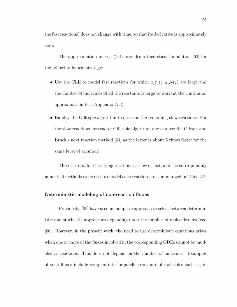
The approximation in Eq. (2.4) provides a theoretical foundation [62] for
the following hybrid strategy:
• Use the CLE to model fast reactions for which ajτ (j ∈ Mf ) are large and
the number of molecules of all the reactants is large to warrant the continuum
approximation (see Appendix A.3).
• Employ the Gillespie algorithm to describe the remaining slow reactions. For
the slow reactions, instead of Gillespie algorithm one can use the Gibson and
Bruck’s next reaction method [64] as the latter is about 5 times faster for the
same level of accuracy.
These criteria for classifying reactions as slow or fast, and the corresponding
numerical methods to be used to model each reaction, are summarized in Table 2.2.
Deterministic modeling of non-reaction fluxes
Previously, [65] have used an adaptive approach to select between determin-
istic and stochastic approaches depending upon the number of molecules involved
[66]. However, in the present work, the need to use deterministic equations arises
when one or more of the fluxes involved in the corresponding ODEs cannot be mod-
eled as reactions. This does not depend on the number of molecules. Examples
of such fluxes include complex inter-organelle transport of molecules such as, in

26
our model, movement of Ca2+ from endoplasmic reticulum to the cytosol through
IP3R channels (Jch in Eq. (2.5)). One can argue that this particular flux could
be modeled using the 12 reversible reactions proposed by [67] and later simplified
by [59]. However, in some cases the detailed mechanisms are not known and flux
approximation is the only option.
The calcium dynamics model [9] includes four coupled ODEs for the state
variables [Ca2+]ER, [Ca2+]i, h and [Ca2+]mit, which contain fluxes whose under-
lying mechanisms involve many reactions that are not modeled explicitly. These
processes are treated deterministically in our algorithms. Consider, for example,
the rate of change of [Ca2+]ER (the other three ODEs can be found here [9]),
d[Ca2+]ER
dt=βER
ρER
(JSERCA − Jch − JER,leak). (2.5)
In Eq. (2.5), the rapid binding of calcium to buffer proteins is modeled implicitly
through βER, the ratio of free calcium to total (free and bound) calcium in the ER;
and the use of ρER, the volumetric ratio of the ER and the cytosol, obviates the
need to specify the ER volume explicitly. The calcium fluxes through the SERCA
pump back to the ER, JSERCA, through the IP3R channel from the ER to the
cytosol, Jch, and due to the calcium leakage from the ER, JER,leak, are prescribed
as nonlinear functions of the state variables [Ca2+]ER, [Ca2+]i, h and [Ca2+]mit.
The complexity of the fluxes of the state variables [Ca2+]ER, [Ca2+]i, h
and [Ca2+]mit complicate their modeling with the stochastic simulation algorithms
described above. For example, the expression for Jch is given by:

27
Jch = vmax,ch×([
[IP3]
[IP3] +KIP3
]×[
[Ca2+]i
[Ca2+]i +Kact
]× h)
3× ([Ca2+]ER− [Ca2+]i)
(2.6)
So, in our hybrid approach, the corresponding four ODEs are integrated
via a first-order Euler scheme after all other quantities are updated using the
multi-scale stochastic method described in Section 2.3.3. The coupling of con-
tinuum (ODE-based) and stochastic (particle-based) descriptions requires relating
the concentrations to numbers of molecules. For the cytosolic calcium dynamics
in RAW 264.7 cells considered in this study, we use a cytosolic volume V = 10pL
or a cell diameter of 27µm. Then the concentrations, e.g., the concentration of
ligand, [L] = 30nM, can be related to the numbers of molecules, as follows
30nM = 30× 10−9 × 6.022× 1023
L× 10−11L = 180, 660 molecules. (2.7)
Reactions with complex rate expressions
Some explicitly modeled reactions have complex rate laws which are ac-
tually functions of Michaelis-Menten (M-M) or Hill dynamics-based complex rate
expressions.
We studied four methods for stochastic simulation presented in the litera-
ture to perform course-graining and handle complex rate laws such as Michaelis-
Menten rate law for a single reaction and coupled reactions with Michaelis-Menten
rate law. The first such contribution is the quasi-steady-state approximation

28
(QSSA) approach of [22]. [68] have carried out in-depth analysis of using QSSA
under different conditions through the use of singular perturbation analysis. More
recently, [27] have extended the QSSA by analyzing the conditions under which the
standard QSSA might fail. They have utilized the total QSSA (TQSSA) and have
shown that under certain conditions the method of [22] fails. They have applied
the TQSSA approach to a single Michaelis-Menten mechanism, the Goldbeter-
Koshland (GK) ultrasensitive switch system involving two coupled Michaelis-Menten
mechanisms and a bistable system composed of two GK switches. The approach
requires solving quadratic equations to solve for the propensity for slow reactions
for use with the standard Gillespie algorithm. For these cases, the results are out-
standing in that the mean temporal responses obtained from the TQSSA and the
standard Gillespie algorithm are indistinguishable. The work of [32] deals with
a detailed analysis of the issues in simplification of Michaelis-Menten formulation
into a single-step reaction in stochastic simulation.
All these are successful approaches in handling systems with one or a few
reactions. However, these approaches have not been applied on more complex
systems involving many reactions (say, about 20 or more) with both simple and
complex rate laws. Some of the rate laws in our model are much more complex
than even the most complex examples presented in these contributions because in
our case, the corresponding mechanisms are highly lumped representations of the
underlying detailed mechanisms. If one were to consider the detailed mechanisms,
the parameters would be unknown.
29
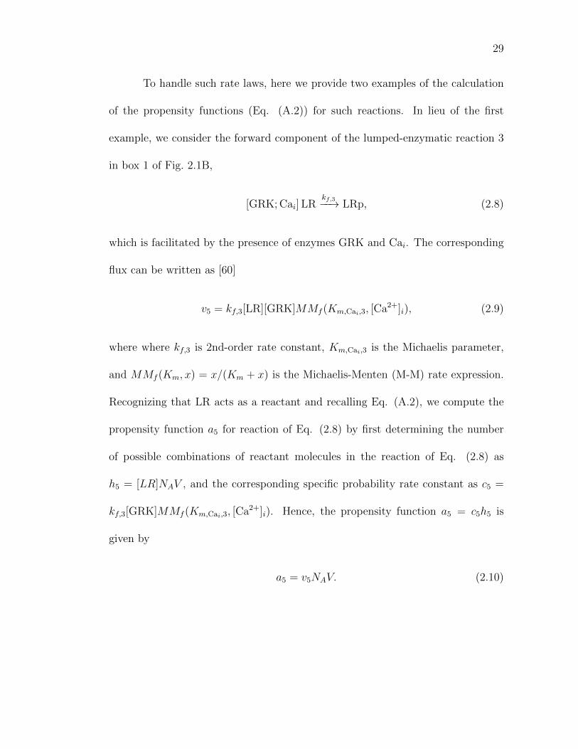
To handle such rate laws, here we provide two examples of the calculation
of the propensity functions (Eq. (A.2)) for such reactions. In lieu of the first
example, we consider the forward component of the lumped-enzymatic reaction 3
in box 1 of Fig. 2.1B,
[GRK; Cai] LRkf,3−−→ LRp, (2.8)
which is facilitated by the presence of enzymes GRK and Cai. The corresponding
flux can be written as [60]
v5 = kf,3[LR][GRK]MMf (Km,Cai,3, [Ca2+]i), (2.9)
where where kf,3 is 2nd-order rate constant, Km,Cai,3 is the Michaelis parameter,
and MMf (Km, x) = x/(Km + x) is the Michaelis-Menten (M-M) rate expression.
Recognizing that LR acts as a reactant and recalling Eq. (A.2), we compute the
propensity function a5 for reaction of Eq. (2.8) by first determining the number
of possible combinations of reactant molecules in the reaction of Eq. (2.8) as
h5 = [LR]NAV , and the corresponding specific probability rate constant as c5 =
kf,3[GRK]MMf (Km,Cai,3, [Ca2+]i). Hence, the propensity function a5 = c5h5 is
given by
a5 = v5NAV. (2.10)
30
2.3.4 Application to cytosolic calcium dynamics in RAW
cells
This multi-scale hybrid approach was applied to the cystolic calcium dy-
namics with parameter values and initial conditions taken from [9]. The system
consists of 28 irreversible reactions and 26 species, which are represented by the
state vector
X = [L,R,LR,Gβγ,GRK,GRK.Gβγ,Ca2+i ,LRp,Rp,LRi,ARR,Rp,i,Rpool,
GiD,T,Gα,iT,Gα,iD,A,PIP2, IP3,PLCβ, IP3p,XPIP2,gen,CaM,
Ca2.CaM,Ca2.CaM.GRK]T . (2.11)
The multi-scale hybrid algorithm is needed because the numbers of molecules of
some of these species are close to 0 while others have above 106 molecules, and
because the propensity functions aj(X) (j = 1, . . . , 28) vary from 0 to over 104.
Before the ligand is added, the system is simulated for 1000 sec so that the
system reaches a steady state. At time t = 1000 sec, ligand C5a is applied to cells
and binds to its receptor (C5aR), which leads to the increase in IP3 levels. The
simulation consists of two phases: before adding ligand and after adding ligand. At
t = 0, the species R, Gβγ, GRK, Ca2+i , Rpool, T, Gα,iD, A, PIP2, PLCβ, XPIP2,gen
and CaM are present. Other species have zero concentration.
At the first time step, τ = 8.0361 × 10⁻⁷ sec. Reactions 14, 17, 18 and 21
in Fig. 2.1B are considered to be fast, while the remaining reactions are taken to
be slow (see approximation 2.2b). The second time step is calculated based on the
31
reaction rates and number of molecules obtained from first time step, etc.
All simulations reported in Section 2.4 were carried out on the linux-based
Triton Cluster at San Diego Supercomputer Center (SDSC), with parallelization
accomplished by using Microsoft’s Star-P program. The number of processors used
varied between 8 and 256 depending upon the number of realizations generated.
On an average, the simulation time for each realization was 15 hrs. The total
single-processor equivalent of simulation time for all the results is about 50,000
hrs.
2.4 Results
Comparison of response of Ca2+i from stochastic and deterministic simula-
tion is presented in Section 2.1. Briefly, in the limit of large number of molecules of
reacting species, stochastic and deterministic simulations yield nearly identical re-
sults. Below, we compare other features of the response as predicted by stochastic
versus deterministic simulation.
2.4.1 Dose response
Dose response, which is a measure of efficacy of a ligand [9], is presented in
Fig. 2.3. Rather than relying on commonly used saturating dose levels to generate
dose-response curves, we choose only sub-basal (very low) doses. This enables us to
identify differences between the dose responses of [Ca2+]i predicted by deterministic

32
and stochastic simulations, respectively. Fig. 2.3A demonstrates the temporal
evolution of the dose responses of [Ca2+]i to the basal dose of [C5a] = 30 nM and
its 0.1%, 1%, 10%, and 50% fractions. The peak height of cytosolic Ca2+ increases
with the dose of ligand, a finding that is made explicit in Fig. 2.3C.
The stochasticity effects and differences in [Ca2+]i responses obtained from
the deterministic and stochastic simulations are explored in Figs. 2.3B and 2.3C.
Note that in Fig. 2.3A the dose responses computed with the two approaches
are nearly identical, with the deterministic predictions shifted to the right by 100
sec to improve visibility. Fig. 2.3B demonstrates the importance of stochasticity
(randomness) for small numbers of ligand molecules (e.g., 0.1% C5a), when the
peak height varies substantially between realizations. Although the ensemble mean
of the peak-height of [Ca2+]i response from these realizations visually overlaps with
that from deterministic prediction, quantitatively, they are different as expressed
through “normalized response difference (NRD)” in Fig. 2.3C.
As the number of molecules becomes very small, the concept of “concen-
tration” loses its rigor and deterministic simulations can be expected to introduce
modeling errors. This effect is elucidated in Fig. 2.3D, where the relative er-
ror or “normalized response difference (NRD)” (E) between the deterministic and
stochastic solutions of [Ca2+]i response is shown. E is computed as,
E ≡ |deterministic− ensemble avg|max(deterministic,ensemble avg)
× 100%. (2.12)
Fig. 2.3D shows that E decreases as the dose of C5a increases, indicating the di-

33
minishing effects of randomness (stochasticity). The NRD varies from E = 7% at
the 0.1% dose to almost zero at the full dose of 30 nM. These results demonstrate
that at lower doses, stochastic simulations are needed and that the ensemble av-
erage of multiple realizations provides a more accurate prediction of the system
behavior then does the deterministic output. Further analysis of this phenomenon
is presented below.
2.4.2 Convergence of stochastic simulations at low doses
Figs. 2.4A-D show the histograms of the peak-value of calcium response,
[Ca2+]i, due to the 0.1% dose of C5a. The histograms in Figs. 2.4A-D represent
respectively 16, 64, 256, and 512 realizations of the stochastic hybrid algorithm,
using 20 bins in each case. The vertical dotted line in each panel corresponds to
the mean computed from the corresponding number of realizations, and the solid
curves are the Gaussian distributions whose mean and variance are computed
from the same realizations. Although the central limit theorem applies to the
distribution of the mean of a random variable instead of the distribution of the
random variable itself, it is interesting to note that the shape of the computed
distributions approaches the Gaussian distribution as the number of realizations
increases from 16 in Figs. 2.4A to 512 in Figs. 2.4D.
To find out if the central limit theorem is applicable to the peak-value of
[Ca2+]i response, the mean of 4, 8, 16 or 32 realizations was computed. This was
repeated in each case to generate 1024 such mean values. The histogram of the
34
mean values is shown in Figs. 2.4E-H. All the four histograms are similar to a
Gaussian distribution and the standard deviation from these distributions indeed
decreased proportional to 1/√Nr, Nr being the number of realizations used to
compute the mean.
2.4.3 Random variability of the [Ca2+]i response at low doses
The number of molecules of C5a at 0.1% dose is about 180. The number of
molecules of cytosolic Ca2+ is of the order of 300,000. The number of molecules
of free Gβγis about 10,000 and that of the phosphorylated receptor still bound
to the ligand (LRp) is about 60. Fig. 2.4I shows how standard deviation (σ) of
the [Ca2+]i response varies across 16 realizations. Fig. 2.4J shows the variation
of the normalized standard deviation σ, defined as: σ = σ/H, where H = h − b
is the difference between the basal level of calcium response b and the peak level
h. It is clear from Fig. 2.4J that the normalized standard deviation σ increases
as the C5a dose decreases, indicating the increasing importance of randomness
(stochasticity). This is because as the C5a dose (the number of C5a molecules)
decreases, fewer C5a molecules participate in chemical collisions and hence the
enhanced relative importance of stochasticity. One implication of this is that more
stochastic realizations are needed to accurately estimate the mean response or the
variability in response. From experimental view point, a larger population of cells
is needed to get a stable reading for mean calcium response.

35
2.4.4 Sensitivity analysis
In this study we have focused on the perturbations in the initial pool of
certain species. Quantification of parametric uncertainty in the reaction rate con-
stants used in the Gillespie and other algorithms described above can be carried
out following the procedure described in [69]. A similar analysis could be per-
formed with respect to perturbations in the rate parameters while keeping the C5a
dose and the initial pool of all species at their nominal levels. Since the number
of molecules is sufficiently large under these conditions, the results of sensitivity
analysis using stochastic simulation are similar to those obtained using determin-
istic simulation. As an example, results of sensitivity analysis of [Ca2+]i response
for changes in k1.
The sensitivity of [Ca2+]i response to variations in [Gβγ] is shown in Fig. 2.5.
In this discussion, IC refers to initial condition, which is generally also the total
pool of protein/species being considered. These concentrations were changed, one
at a time, by factors of 10−3, 10−2, 0.05, 0.1, 0,2, 0.5, and 0.75 of their respective
base values. For each concentration change, a new basal level (steady state) was
computed by allowing the system to evolve for 1000 sec before ligand addition, at
which time 30 nM of C5a ligand was applied. Note that 10% of a base value means
a 90% knockdown of the species/gene in question. Shift of basal level before ligand
addition and the peak-height from basal level are the main focus of this sensitivity
analysis.
36
Figs. 2.5A-C provide an analysis of the [Ca2+]i response to changing doses of
IC:[Gβγ], which varies from its base value to the 1/20, 1/5, 1/2, and 3/4 fractions
thereof. The number of molecules involved at 1/20 level of IC:[Gβγ] is: Gα,iD:
46,000, Gα,iT: 5,100, free Gβγ: 16, GRK.Gβγ: 10, LRp, 1,400, Rp, 15, IP3: 260,000
and free cytosolic Ca2+: 290,000. Figs. 2.5B-C reveal that the [Ca2+]i response
is very sensitive to the changes in IC:[Gβγ]. Its peak height decreases by 90%
as IC:[Gβγ] is reduced by 50%, and becomes negligible when [Gβγ] drops below
20% of its base value (Fig. 2.5B). The relative error between the [Ca2+]i responses
predicted by deterministic and stochastic simulations, E (Fig. 2.5C) becomes very
large when the concentration [Gβγ] drops below 20% of its base value, indicating
the importance of randomness, which is caused by small numbers of molecules of
Gβγ.
We have also studied how the mean peak-height and NRD change when
different numbers of realizations are used. Fig. 2.5B show the mean peak-height
obtained from 8, 16, 32 realizations and deterministic simulation. The curves are
almost indistinguishable. Difference for [5%, 20%, 50%, 75%, 100%] of IC:[Gβγ]
is [1.1775 0.15677 0.16032 0.10425 0.10491]%; the large difference being less than
1.2%. Essentially, 16 realizations are sufficient to compute the mean with good
accuracy that is what is used in other simulations as well.
37
2.4.5 Calcium response to protein knockdown
Since the stochastic hybrid algorithm enables us to predict cytosolic calcium
dynamics when only a few molecules of reacting species are present, we are in a
position to explore the effects of proteins’ knockdown on calcium response. Figs. 2.6
and 2.7 show the [Ca2+]i response to knockdown of proteins PLCβ and GRK,
respectively. Fig. 2.8 shows the [Ca2+]i response to knockdown of protein GRK
and perturbation of (knockdown of the protein related to) Vmax,PM,IP3dep. To model
a protein’s knockdown, we first reduced its basal level, and then computed a new
basal level (steady state) by evolving the system for 1000 sec, at which time 30
nM of C5a ligand was applied.
Figs. 2.6A and 2.6B show the [Ca2+]i response to the 50%, 80%, 90%,
and 99% knockdown of PLCβ for 0.1% and 10% doses of IC:[R], respectively.
The number of molecules involved at 0.1% dose of IC:[R] and 90% knockdown
of PLCβ is: total PLCβ: 3,400, Gα,iD: 17,000, Gα,iT: 350, free Gβγ: 14,000,
GRK.Gβγ: 3,700, LRp, 225, Rp, 2, IP3: 270,000 and free cytosolic Ca2+: 297,000.
Fig. 2.6C provides a temporal snapshot of the [Ca2+]i peak heights corresponding
to different combinations of the PLCβ and IC:[R] levels. Both the peak height
and basal levels of [Ca2+]i decrease as the knockdown level of PLCβ increases.
The deterministic and stochastic simulations yield similar results with NRD less
than 4% (Fig. 2.6D). This clearly suggests that it may not be necessary to carry
out stochastic simulation to model knockdown of PLCβ. For experiments, the

38
implication is that a relatively smaller population of cells may be sufficient to get
a stable readout if other experimental factors can be controlled.
Figs. 2.7A and 2.7B present the [Ca2+]i response to the 50%, 80%, 90%,
and 99% knockdown of GRK for 0.1% and 10% doses of IC:[R], respectively. The
number of molecules involved at 0.1% dose of IC:[R] and 90% knockdown of GRK
is: free GRK: 1,500, Gα,iD: 9,200, Gα,iT: 400, free Gβγ: 10,000, GRK.Gβγ: 400,
LRp, 44, Rp, 1, IP3: 400,000 and free cytosolic Ca2+: 301,000. The largest peak
height occurs at lowest [GRK] and highest [R] (Fig. 2.7C), which is qualitatively
opposite to the response due to the PLCβ. Fig. 2.7D demonstrates that either
deterministic or stochastic simulations can be used to investigate this behavior,
with the maximum NRD E of about 1.5%, which occurs at low [R] and is practically
independent of the level of GRK.
Fig. 2.8 demonstrates the [Ca2+]i response to various degrees of simul-
taneous knockdown of protein GRK and the protein related to Vmax,PM,IP3dep.
Knockdown of GRK has a more pronounced effect on [Ca2+]i response than does
Vmax,PM,IP3dep. The relative importance of the two knockdowns does not change at
different levels of KD. This suggests the robustness of the system response over a
large range of perturbations.

39
2.5 Summary and Discussion
In summary, we have integrated the existing techniques for multiscale stochas-
tic simulation with deterministic simulation to deal with complex reactions systems
and have applied it to studying calcium dynamics in macrophage cells. When the
concentration of reactants is sufficiently large, the stochastic method yields time-
course profiles identical to those obtained from a deterministic model (ensemble
average of 16 or more realizations). However, at lower number of molecules of one
or more species, measurable relative difference in [Ca2+]i responses predicted by
the two approaches is obtained, especially for the case of Gβγ, thus suggesting the
necessity of using stochastic simulation as opposed to deterministic simulation for
studying system dynamics at sub-cellular levels. Dose response analysis revealed
that while the normalized response difference (NRD) between [Ca2+]i responses
predicted by deterministic and stochastic simulations is negligible at the full dose
of 30nM (shown) or higher doses including saturating doses (not shown), it in-
creases with decreasing doses. At 0.1% dose, it is as high as 7%. These results
are emphasized again in the sensitivity analysis of the parameters used in the
simulation and in the knockdown analysis of reacting protein components.
2.5.1 Methodological novelty
We have developed a hybrid approach to stochastic simulation, in which
slow reactions and fluxes are handled through exact stochastic simulation and

40
their fast counterparts are treated partially deterministically through the chemical
Langevin equation. The classification of reactions as fast or slow is accompanied by
a partial equilibrium assumption, according to which a population of slow species
is not altered by fast reactions. Our new approach also handles reactions with com-
plex rate expressions such as functions of Michaelis-Menten kinetics and power-law
kinetics by developing mathematical expressions for their propensity functions and
microscopic fluxes. Fluxes which cannot be modeled explicitly through reactions
are handled deterministically.
2.5.2 Sensitivity analysis
With decreasing IC:[R], lesser [Gβγ] is available [42] (Figs. 2.5A-C), which
results in reduced activation of PLCβ and as a consequence reduced hydrolysis of
PIP2 into IP3. Hence, the increase in cytosolic [Ca2+] is smaller. The sensitivity
curve for IC:[R] in Fig. 2.5B is nonlinear. This is because the ligand and the
receptor bind in 1:1 stoichiometry, and the nominal value of IC:[R] (∼40nM) is
larger than the nominal (100%) level of C5a (30nM). Thus, for a small decrease
(say, 10%) in IC:[R], about 36nM [R] is present. Since 36nM is still larger than
30nM, the dynamics of [LR] remains almost the same and so does the peak height
of the temporal response of [Ca2+]i. Basal level does not change in our model since
the receptor comes into play only after adding the ligand. In reality, there is a little
decrease of [Ca2+] in cytosol due to the little basal activity, but it is compensated
by the basal hydrolysis rate of PIP2 and hence is unobservable.
41
The peak height of the [Ca2+]i response decreases with decreasing value of
IC:[Gβγ], and no baseline shift is observed (Fig. 2.5D). In the absence of perturba-
tion, at early times, the concentrations [Gβγ] = 8.28e−3 µM and [Gα,iD] = 8.12e−3
µM are almost equal. However, if IC:[Gβγ] is decreased, there is little free Gβγ left.
Since this directly affects the rate of PIP2 hydrolysis, no IP3 can be generated. Due
to this effect, with decreasing IC:[Gβγ], the peak-height of [Ca2+]i decreases much
more sharply. Although not shown in Figs. 2.5D-E, if IC:[Gβγ] increases beyond
100% of base case, then the excess Gβγ is present in the free form, hence both the
basal level and peak-height increase till saturation. This is similar to the decrease
in IC:[Gα,iD] shown in Figs. 2.5G-I and briefly discussed below.
Sensitivity analysis of IC:[Gα,iD] shows biphasic response of [Ca2+]i: large
baseline shift and low peak height at substantially low IC:[Gα,iD] (Fig. 2.5G, upper
panel) and a small baseline shift (increase) and the corresponding nominal increase
of peak height at relatively smaller perturbations ([90% 85% 80%] of IC:[Gα,iD],
Fig. 2.5G, lower panel). At substantially low [Gα,iD], large amount of free [Gβγ]
results in a large basal level shift and with the basal level at this plateau, little
additional increase in [Ca2+]i is observed, i.e. this results in a low peak-height of
[Ca2+]i upon ligand addition.
The NRD increases with decreasing IC:[R]. The behavior of NRD for de-
crease in IC:[Gβγ] is similar to that for decrease in IC:[R] except that it is drastically
larger at very low values (more than 80% NRD at 5% IC:[Gβγ]). While the NRD
in the sensitivity analysis of IC:[R] is under 2% for all changes, it is up to 90% in
42
the perturbation of IC:[Gβγ]. There are three reasons for this drastic difference:
(1) stochastic effects are prominent at low concentrations, (2) the system is very
sensitive to large decreases in [Gβγ] as compared to in [R] or [Gα,iD], and (3) the
NRD is normalized by the peak-height (Eq. (2.12)). Since peak-height is very low
at low [Gβγ], the NRD gets amplified.
2.5.3 Knockdown (KD) analysis
Our results show reduced G-protein activity and [Ca2+]i response upon
KD of the receptor. KD of Gβγ results in a sharp decrease in calcium levels
and KD of Gα,iD results in considerably large increases in basal level of [Ca2+]i
(inferred from sensitivity analysis). KD of GRK results in increased and prolonged
mobilization of calcium since the receptor remains active for a longer time. Thus,
GRK regulates G-protein activity strongly. Similar to Gβγ, knockdown of PLCβ
shows a sharp decrease in [Ca2+]i. This is because IP3 generation is catalyzed by
the active complex of Ca2+, PLCβ and Gβγ. As the knockdown level of PLCβ
increases, both the peak height and basal levels of [Ca2+]i decrease since less IP3
is generated. Qualitatively, the knockdown response of PLCβ is similar to that of
the knockdown response of Gβγ since both play a similar role in IP3 generation.
In contrast to the KD response of PLCβ, as KD level of GRK increases,
peak height of [Ca2+]i increases strongly (Figs. 2.7A-B). This is because the phos-
phorylation induced through reactions 3 and 4 decreases as KD level of GRK
increases. Moreover, the time to return to steady state also increases considerably

43
since the receptor remains active for longer time and relatively more Gβγ is present
in the free active state. The basal level increases slightly relative to peak-height
only at low IC:[R] (0.1%, Fig. 2.7A). At moderate IC:[R] (10%, Fig. 2.7B), the
increase in basal level is negligible as compared to the peak-height.
Vmax,PM,IP3dep affects JPM,IP3dep (IP3-dependent in-flux to cytosol across the
plasma membrane) in a proportional manner. Double perturbation of GRK and
Vmax,PM,IP3dep has revealed that for increase in their KD levels, GRK and Vmax,PM,IP3dep
have opposite effects on [Ca2+]i. Reduction of Vmax,PM,IP3dep results in decrease of
[Ca2+]i because JPM,IP3dep is reduced (the lower three time-courses shown with light
colored lines in Fig. 2.8). On the contrary, KD of GRK increases [Ca2+]i response
because phosphorylation of the active receptor is reduced (Fig. 2.8, time-course
shown with light continuous line (100% Vmax,PM,IP3dep and 100% GRK) and time-
course shown with dark continuous line (100% Vmax,PM,IP3dep and 50% GRK)). The
qualitative nature of the response does not change at different KD levels of the
protein GRK and the protein related to Vmax,PM,IP3dep suggesting that the system
is robust to such perturbations.
The main features of the KD response are summarized in Table 2.3.
2.5.4 Stochastic effects at low molecular numbers
In the base case (30nM C5a), there is good agreement between [Ca2+]i
responses predicted by deterministic and stochastic simulation. However, at low
doses of the ligand or proteins such as the receptor and GRK, stochastic effects
44
become prominent resulting in up to 2-4% NRD for low concentrations of the
receptor, GRK and Gα,iD, up to 7% NRD for dose response and up to 90% NRD
for low concentration of Gβγ. Although the absolute value of fluctuations is larger
in the case of higher doses resulting in a higher peak [Ca2+]i value, the normalized
standard deviation of the response increases with decreasing dose.
2.5.5 Deriving statistics from stochastic simulation
We also found that with more realizations, the computed distribution of
the ensemble mean of the peak-height approaches a normal distribution when the
number of realizations used to compute the mean increases, as would be mandated
by the central limit theorem. Our results suggest that when 20 bins are used,
about 250 realizations are sufficient to derive an approximate distribution; results
from 512 realizations are good in terms of reaching a normal distribution. Statis-
tics related to low order moments of the distribution, such as mean and standard
deviation could be computed accurately even with lesser number of realizations
(about 16 realizations to compute the mean and about 128 realizations for the
standard deviation) at least for the cytosolic calcium response. For other systems
some trial may be involved. These results can be potentially used for deciding
the number of realizations needed to compute meaningful statistics in stochastic
simulations, at least for similar systems with a similar number of components.

45
TaiJung Choi, Mano R. Maurya, Daniel M. Tartakovsky, Shankar Subra-
maniam (2010), ‘Stochastic Hybrid Modeling of Intracellular Calcium Dynamics’.
J. Chem. Phys., 133, 165101

46
Table 2.1: The run-time scalability of the Gillespie, tau-leap, and chemical
Langevin equation algorithms as a function of the number of molecules.
Initial number of moleculesS: 312, E: 125 S: 31200, E: 12500
Method Computation time (s) Computation time (s)Gillespie algorithm 0.892 100.3Tau-leap algorithm 0.235 0.354
CLE 0.003 0.003
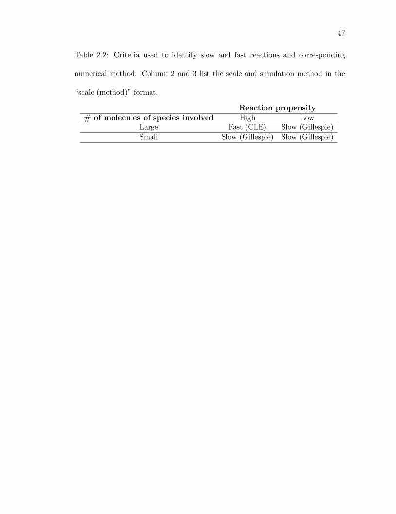
47
Table 2.2: Criteria used to identify slow and fast reactions and corresponding
numerical method. Column 2 and 3 list the scale and simulation method in the
“scale (method)” format.
Reaction propensity# of molecules of species involved High Low
Large Fast (CLE) Slow (Gillespie)Small Slow (Gillespie) Slow (Gillespie)
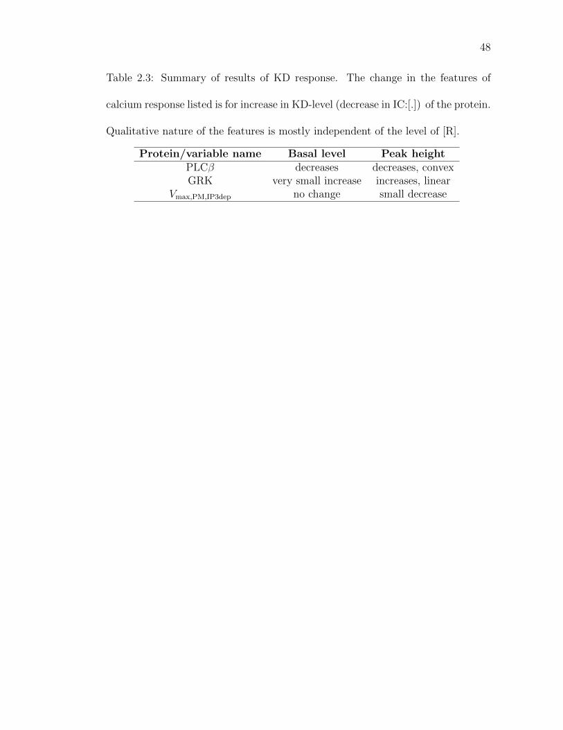
48
Table 2.3: Summary of results of KD response. The change in the features of
calcium response listed is for increase in KD-level (decrease in IC:[.]) of the protein.
Qualitative nature of the features is mostly independent of the level of [R].
Protein/variable name Basal level Peak heightPLCβ decreases decreases, convexGRK very small increase increases, linear
Vmax,PM,IP3dep no change small decrease

49
GTPase activating protein (GAP), respectively. Reaction 15 is similar to
reaction 12 but is catalyzed by L.R, and reaction 16 is similar to reaction 13
but is catalyzed by GAP (A, RGS) (57). A more detailed description of theGTPase cycle, similar to the three-cube model in Fig. 1 A of Bornheimer
et al. (58) but with simplification of reactions GD4G4GT into GD4GT
(Fig. 1 B, reaction 12) and explicit modeling of Gbg and Ga,i, was included
in a detailed model, but its fit to one set of basic experimental data(stimulation with 250 nMC5a) was similar to the compact model of Fig. 1 B.Hence, to reduce computational complexity, only the simpler model (Fig.
1 B) is used for further analysis with knockdown data. Additional discussionon this simplification is presented in Supplementary Material (Approxima-tions and the lumped/simplified mechanisms in the model). Reactions 15 and
16 are lumped-enzymatic reactions, where T is GTP, D is GDP, and A is the
GAP RGS.
Reaction 15: !L:R"GiD1T/Ga;iT1Gbg 1D
#L:R is an enzyme$Reaction 16: !A"Ga;iT/Ga;iD1 Pi #A is an enzyme$
IP3 module. In the basal state, most of the IP3 is generated due to slowhydrolysis of PIP2 (reaction 17), since free Gbg is present in very small
amounts. Upon G-protein activation, dissociated Gbg binds to PLCb. CytosolicCa21 (Fig. 1 B, box 3, Cai) can bind to both PLCb and PLCb.Gbg. Bind-ing affinities for Gbg and calcium-bound forms of PLCb are ;10 times
higher than that of free PLCb (13). Each of PLCb.Gbg, PLCb.Cai andPLCb.Gbg.Cai catalyze hydrolysis of PIP2, but PLCb.Gbg.Cai is the most
potent. In our model, for simplification, a lumped-enzymatic reaction isused to model the enhancement due to PLCb.Gbg.Cai (see reaction 18 (Fig.
1 B, box 3)):
Reaction 18: !Cai; Gbg; PLCb" PIP2/IP3 1DAG
#enzyme is a ternary complex of Cai; Gbg; and PLCb$:
As explained in Supplementary Material (Approximations and the
lumped/simplified mechanisms in the model), the rate expression of theabove reaction is a close approximation to an expression derived based on
the assumption that all the four reversible reactions related to PLCb are in
equilibrium. Further, it is assumed that the enzymatic effect of PLCb.Gbg
and PLCb.Cai is captured through suitable increase in the value of the rate
constant. The amount of Gbg bound to PLCb complexes (estimated to be
;10% of free Gbg) is ignored for Gbg balance (Supplementary Material,
Details of explicitly modeled reactions) in the reduced model; if all otherspecies are included, then little reduction is achieved, and therefore it would
be appropriate to model all reactions explicitly. Since PLCb is not used in
any other reaction in our model, PLCb denotes the total PLCb (buffered).
Reactions 19 and 20 (Fig. 1 A) are simplified and highly lumped repre-sentations of IP3 metabolism, i.e., degradation/conversion to/from other ino-
sitol phosphates and back to PIP2, with only one intermediate pseudospecies,
namely, IP3,p or IP3 product (12). Since oscillation is not observed in theexperimental data on C5a stimulation of RAW cells, this simple represen-
tation is considered sufficient. As Mishra and Bhalla (13) have noted, such a
simple description may be insufficient to model oscillatory response, even
though Marhl et al. (59) have shown that interactions with the mitochondria(included in our model) can result in oscillations, especially above cytosolic
[Ca21] of ;0.5 mM.
It should be noted here that the free Gbg subunit is responsible for the
activation of PLCb, as opposed to activation by the free a subunit of aG-protein, e.g., GaqT (G-protein Gq) upon activation of P2Y2 receptors, as
presented by Lemon et al. (12). For the G-protein Gi, the a subunit, i.e.,
GaiT, does not bind to PLCb. Gbg also has been implicated in calcium
oscillations during fertilization (60).
FIGURE 1 A simplified model for
calcium signaling including calcium in-
flux, ER, and mitochondrial exchange
and storage, used in the conceptual-model-based computation. (A) Overall
schematic model. The ligand C5a binds
to its receptor C5aR on the plasma mem-
brane, activating G-protein Gi. Thefree subunit Gbg binds to and activates
PLCb, which hydrolyzes PIP2 into IP3and DAG. IP3 binds to its receptor on theER membrane and the IP3R channels
open to release calcium into the cytosol.
Other calcium fluxes (e.g., with mito-
chondria and extracellular space) arealso shown. (B) The mechanisms for the
receptor module (box 1), the GTPase
cycle module (box 2), and IP3-generationmodule (box 3), and the feedback effects(boxes 1 and 4). PIP2, phosphatidylino-sitol 4,5-bisphosphate; IP3, inositol 1,4,5-
trisphosphate; IP3R, IP3 receptor; IP3,p, alumped product of IP3 phosphorylation;
Cai, cytosolic Ca21; ER, endoplasmic
reticulum; CICR, calcium-induced cal-
cium release; SERCA, sarco(endo)plasmic reticulum calcium ATPase;
PMCA, plasma membrane calcium
ATPase; NCX, Na1/Ca21 exchanger;mit (subscript), mitochondria; L, ligand C5a; R, receptor C5aR; GRK, G-protein-coupled receptor kinase; CaM, calmodulin; PLCb, phospholipase C-b; GAP,GTPase activating protein; RGS, regulator of G-protein signaling; DAG, diacylglycerol; PKC, protein kinase C; Pi, phosphate.
712 Maurya and Subramaniam
Biophysical Journal 93(3) 709–728
(A) Overall schematic (B) Modules
ADP
ATPSERCApump
mitochondria
IP3IP3,P
PIP2
Leak IP3 dependentflux
PMR
Figure 2.1: A simplified model for calcium signaling including calcium influx, ER,
and mitochondrial exchange and storage. (A) Ligand C5a binds to its receptor on
plasma membrane (PM) and activates G protein Gi. The free Gβγ binds to PLCβ
and increases its activity which accelerates the phosphorylation of PIP2 into IP3
and DAG. IP3 binds to its receptor IP3R on the ER membrane. Thus, calcium from
the ER is released into the cytosol. Other fluxes between cytosol and mitochondria
or ECM are also shown. (B) Receptor module (box 1), GTPase cycle module (box
2), IP3 generation module (box 3) and feedback module (box 4).
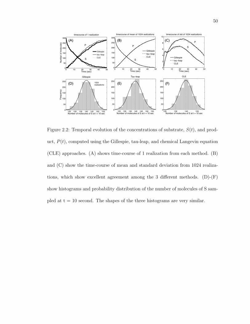
50
125 130 135 140 145 150 1550
50
100
150
200
250
Number of molecules of S at t = 10 sec
Freq
uenc
y
Gillespie
125 130 135 140 145 150 1550
50
100
150
200
250
Number of molecules of S at t = 10 sec
Tau leap
120 130 140 1500
50
100
150
200
250
Number of molecules of S at t = 10 sec
CLE
0 10 20 30 40 500
50
100
150
200
250
300
Time (sec)
timecourse of mean of 1024 realizations
Gillespietau leapCLE
0 10 20 30 40 500
2
4
6
8
10
Time (sec)
timecourse of std of 1024 realizations
Gillespietau leapCLE
0 10 20 30 40 500
50
100
150
200
250
300
Time (sec)
Num
ber o
f mol
ecul
es
timecourse of 1 realization
Gillespietau leapCLE
S
P
S
P P
S
1024 realizations
(A) (C)(B)
(D) (E) (F)
Figure 2.2: Temporal evolution of the concentrations of substrate, S(t), and prod-
uct, P (t), computed using the Gillespie, tau-leap, and chemical Langevin equation
(CLE) approaches. (A) shows time-course of 1 realization from each method. (B)
and (C) show the time-course of mean and standard deviation from 1024 realiza-
tions, which show excellent agreement among the 3 different methods. (D)-(F)
show histograms and probability distribution of the number of molecules of S sam-
pled at t = 10 second. The shapes of the three histograms are very similar.

51
10 4 10 3 10 20
0.01
0.02
0.03
0.04
0.05
Dose amount [C5a] (uM)
Peak
hei
ght [
Ca2+
] i (uM
)
Ensemble avg.Deterministic
10 4 10 3 10 20
2
4
6
8
Dose amount [C5a] (uM)N
RD
(%)
1000 1050 1100 1150 12000.04
0.05
0.06
0.07
0.08
0.09
time (sec)
[Ca2+
] i (uM
)
0.1% C5a1%10%50%100%
950 1000 1050 1100 11500.04938
0.04940
0.04942
0.04944
0.04946
0.04948
0.04950
time (sec)
[Ca2+
] i (uM
)
C5a
Ensemble avg.Deterministic
0.1 % C5a
(A) (B)
(C) (D)
Figure 2.3: Dose response. (A) Comparison between ensemble average of 16 re-
alizations and deterministic simulation. For better contrast, the time-course from
deterministic simulation is shifted by 100s. (B) Comparison between ensemble
average and individual realizations in stochastic simulation for 0.1% (of 30nM)
strength of the ligand C5a. (C) Comparison of the dose response (peak heights):
The difference is quite small as compared to the scale of peak-height. (D) At lower
doses, the normalized response difference (NRD) is larger indicating the stochastic
effects. The NRD decreases with increasing dose as the number of the molecules
of C5a becomes several hundreds or more.

52
950 1000 1050 1100 11500
1
x 10 4
time
stan
dard
dev
iatio
n
0.1% C5a1%10%50%
950 1000 1050 1100 11500
0.2
0.4
0.6
0.8
time
norm
aliz
ed
stan
dard
dev
iatio
n
4.9415 4.9425 4.94350
1
2
Freq
uenc
y
4.9405 4.9425 4.94450
2
4
6
4.94 4.942 4.944 4.9460
10
20
30
4.94 4.944 4.9480
20
40
60
0.1% C5a1%10%50%
4.941 4.942 4.943 4.9440
50
100
150Hist of mean of 4 realizations
Freq
uenc
y
4.941 4.942 4.943 4.944 4.9450
50
100
150Hist of mean of 8 realizations
4.941 4.942 4.943 4.944 4.9450
50
100
150Hist of mean of 16 realizations
4.941 4.942 4.943 4.944 4.9450
50
100
150Hist of mean of 32 realizations
Peak value (x10 2)
16 realizations 64 realizations 256 realizations 512 realizations
Peak value (x10 2)
(A) (B) (C) (D)
950 1000 1050 1100 11500
1
x 10 4
timest
anda
rd d
evia
tion
0.1% C5a1%10%50%
950 1000 1050 1100 11500
0.2
0.4
0.6
0.8
time
norm
aliz
ed
stan
dard
dev
iatio
n
4.9415 4.9425 4.94350
1
2
Freq
uenc
y
4.9405 4.9425 4.94450
2
4
6
4.94 4.942 4.944 4.9460
10
20
30
4.94 4.944 4.9480
20
40
60
0.1% C5a1%10%50%
4.941 4.942 4.943 4.9440
50
100
150Hist of mean of 4 realizations
Freq
uenc
y
4.941 4.942 4.943 4.944 4.9450
50
100
150Hist of mean of 8 realizations
4.941 4.942 4.943 4.944 4.9450
50
100
150Hist of mean of 16 realizations
4.941 4.942 4.943 4.944 4.9450
50
100
150Hist of mean of 32 realizations
Peak value (x10 2)
16 realizations 64 realizations 256 realizations 512 realizations
Peak value (x10 2)
(E) (F) (G) (H)
950 1000 1050 1100 11500
1
x 10 4
time
stan
dard
dev
iatio
n
0.1% C5a1%10%50%
950 1000 1050 1100 11500
0.2
0.4
0.6
0.8
time
norm
aliz
ed
stan
dard
dev
iatio
n
4.9415 4.9425 4.94350
1
2
Freq
uenc
y
4.9405 4.9425 4.94450
2
4
6
4.94 4.942 4.944 4.9460
10
20
30
4.94 4.944 4.9480
20
40
60
0.1% C5a1%10%50%
4.941 4.942 4.943 4.9440
50
100
150Hist of mean of 4 realizations
Freq
uenc
y
4.941 4.942 4.943 4.944 4.9450
50
100
150Hist of mean of 8 realizations
4.941 4.942 4.943 4.944 4.9450
50
100
150Hist of mean of 16 realizations
4.941 4.942 4.943 4.944 4.9450
50
100
150Hist of mean of 32 realizations
Peak value (x10 2)
16 realizations 64 realizations 256 realizations 512 realizations
Peak value (x10 2)
(I) (J)
Figure 2.4: Revelation of stochastic effects at low doses. (A)-(D) Distributions of
peak-height for the 0.1% dose of C5a computed from 16, 64, 256, and 512 real-
izations, respectively. The dotted vertical line represents the mean value and the
solid curves denote theoretical Gaussian distributions. As the number of realiza-
tions increases, the shape of the histogram approaches a Gaussian distribution.
(E)-(H) The mean of 4, 8, 16 or 32 realizations was computed. All the four his-
tograms are similar to a Gaussian distribution and the standard deviation from
these distributions indeed decreased proportional to 1/√Nr, Nr being the number
of realizations used to compute the mean. (I) The standard deviation computed
from 16 realizations for several doses. Contrary to the expectation, higher doses
result in larger absolute standard deviations. (J) The normalized standard devia-
tion decreases as the dose is increased, signifying the effect of randomness at lower
doses.

53
1000 1050 1100 11500.04
0.05
0.06
0.07
0.08
0.09
time (sec)
[Ca2+
] i (uM
)
IC:[Gbg]5%IC:[Gbg]
20%50%75%100%
0 0.2 0.4 0.6 0.8 10
0.01
0.02
0.03
0.04
0.05
ratio: IC [Gbg]
Peak
hei
ght [
Ca2+
] i (uM
)
8 runs16 runs32 runsdeterministic
0 0.2 0.4 0.6 0.8 10
20
40
60
80
100
ratio: IC[Gbg]
NR
D (%
)
8runs16runs32runs
(A) (B) (C)
Figure 2.5: Sensitivity analysis. (A)-(C) Response of [Ca2+]i to changes in
IC:[Gβγ]. The decrease in the peak height due to decrease in IC:[Gβγ] is much
more pronounced than that caused by the same decrease of IC:[R]. (C) NRD E is
extremely high at very low IC:[Gβγ], suggesting significant stochastic effects at low
numbers of molecules of [Gβγ]. (B) and (C) also show the effect of using different
number of realizations for computing the mean. Such differences are small (see
text) indicating that 16 realizations are sufficient for computing the mean.

54
950 1000 1050 1100 11500.0486
0.0487
0.0488
0.0489
0.049
0.0491
0.0492
time (sec)
[Ca2+
] i (uM
)
99% KD90%80%50%
950 1000 1050 1100 11500.0485
0.049
0.0495
0.05
0.0505
0.051
0.0515
time (sec)
[Ca2+
] i (uM
)
99% KD90%80%50%
10 2
100
0
0.5
1
0
0.02
0.04
log ratio IC: [R]ratio IC: [PLCb]
peak
hei
ght [
Ca2+
] i (uM
)
10 2
100
0
0.5
1
0
2
4
log ratio IC: [R]ratio IC: [PLCb]
Diffe
renc
e ra
te (%
)
KD of PLCb KD of PLCb(A)
(C) (D)
(B)
NR
D(%
)
0.1% of IC:[R] 10% of IC:[R]
Figure 2.6: Knockdown response of PLCβ. (A)-(B) The [Ca2+]i response to the
50%, 80%, 90%, and 99% knockdown of PLCβ for 0.1% and 10% levels of IC:[R],
respectively. As the knockdown rate of PLCβ increases, both the basal level and
peak height of [Ca2+]i decrease, because the IP3 production decreases due to de-
crease in PLCβ. (C) Peak-height of [Ca2+]i response corresponding to different
combinations of the PLCβ and IC:[R] levels. Peak height increases with high
amount of IC:[R] and [PLCβ]. (D) NRD E is insignificant and decreases as doses
of R and PLCβ increase.

55
950 1000 1050 1100 11500.0494
0.0495
0.0496
0.0497
0.0498
0.0499
0.05
time (sec)
[Ca2+
] i (uM
)
99% KD90%80%50%
950 1000 1050 1100 11500.04
0.05
0.06
0.07
0.08
time (sec)
[Ca2+
] i (uM
)
99% KD90%80%50%
10 2
100
0
0.5
1
0
0.05
0.1
log ratio IC: [R]ratio IC: [GRK]
peak
hei
ght [
Ca2+
] i (uM
)
10 2
100
0
0.5
1
0
1
2
log ratio IC: [R]ratio IC: [GRK]
Diff
eren
ce ra
te (%
)
KD of GRKKD of GRK
(B)(A)
(C) (D)
NR
D(%
)
10% of IC:[R]0.1% of IC:[R]
Figure 2.7: Knockdown response of GRK. (A)-(B) The [Ca2+]i response to the
50%, 80%, 90%, and 99% knockdown of GRK for 0.1% and 10% levels of IC:[R],
respectively. (C) Peak-height of [Ca2+]i response corresponding to different com-
binations of [GRK] and IC:[R] levels. (D) NRD E is insignificant, reaching its
maximum of about 1.5% at low IC:[R].

56
980 1000 1020 1040 1060 1080 1110 11200.04
0.05
0.06
0.07
0.08
0.09
0.1
0.11
0.12
time (sec)
[Ca2+
] i (uM
)
10% Vmax_IP3dep & 100% GRK50% Vmax_IP3dep & 100% GRK10% Vmax_IP3dep & 50% GRK100% Vmax_IP3dep & 50% GRK100% Vmax_IP3dep & 100% GRK
decreaseVmax,IP3,dep
KD of GRK
Figure 2.8: The [Ca2+]i response to the simultaneous knockdown of GRK
and gene/protein related to Vmax,IP3dep. Knockdown of GRK and reduction of
Vmax,PM,IP3dep have opposite effects on the [Ca2+]i response. The response is much
more sensitive to knockdown of GRK than to decrease in Vmax,PM,IP3dep.
Chapter 3
Stochastic Operator Splitting
Approach for Reaction-Diffusion
Processes
3.1 Introduction
Randomness plays an important role in the behavior of many biological phe-
nomena, such as cellular signaling and gene regulatory networks [8, 70, 71]. While
deterministic ordinary differential equations (ODEs) often provide accurate pre-
dictions of the dynamics of biochemical pathways with large numbers of reacting
molecules, they fail when the concentrations of reactants and/or their products
57
58
become small and the law of mass action becomes invalid. When this occurs,
the randomness associated with the dynamics of individual molecules becomes
pronounced, necessitating the use of stochastic simulations. Standard stochastic
techniques, e.g., Gillespie’s stochastic simulation algorithm [11] and its computa-
tionally efficient modifications [12, 72], are routinely used to model biochemical
reactions in such systems. Such algorithms assume that reactants and their prod-
ucts are well-mixed, i.e., distributed uniformly in space.
The latter assumption is problematic when the number of molecules is small.
This is especially so in crowded environments with complex internal geometry,
wherein stochasticity and spatial variability are inseparable. Partial differential
equations (PDEs) provide accurate macroscopic predictions of the dynamics of
spatially heterogeneous systems with large numbers of molecules. Yet, similar to
ODE-based models, they fail to account for the randomness inherent in a system
comprised of small numbers of molecules. It is essential that computational meth-
ods for reaction-diffusion systems with small numbers of molecules are capable of
handling both stochasticity and heterogeneity.
A number of micro- and meso-scale methods have been developed for the
simulation of reaction-diffusion systems. The micro-scale approaches, e.g., the
Green’s function reaction dynamics [14] and Smoldyn’s algorithm [15], are based
on Brownian dynamics and require the reacting molecules to diffuse within a cer-
tain distance from each other in order for bimolecular reactions to take place. The
latter requirement necessitates the use of a numerical mesh and the tracking of in-
59
dividual particles and/or distances between them, which renders such algorithms
computationally expensive. Mesoscopic approaches, e.g., MesoRD [16] and the
Gillespie multi-particle (GMP) method [17, 18], trade representational accuracy
for computational efficiency. They are based on a reaction-diffusion master equa-
tion [19], which generalizes a chemical master equation developed for well-mixed
chemical reactions by discretizing the space into a collection of cells and treating
each cell as a well mixed system. MesoRD [16] treats diffusion as a unimolecular re-
action whose reaction rate is related to the corresponding diffusion coefficient. The
GMP method [17, 18] employs an operator-splitting scheme in which the Gillespie
algorithm and cellular automata [20] handle reactions and diffusion, respectively.
We present a numerical algorithm to simulate stochastic reaction-diffusion
processes with a small number of non-uniformly distributed molecules. It employs
an operator-splitting, in which the Gillespie algorithm (or its accelerated versions)
and Brownian dynamics (or the Smoluchowski equation) are used to simulate re-
actions and diffusion, respectively. Our algorithm is conceptually similar to the
GMP method in that it relies on operator-splitting. However it offers a number
of computational advantages in terms of both accuracy and efficiency. First, the
cellular automata used in the GMP method restrict a particle’s movement during
one fixed time-step to the adjacent cells only; while Brownian motion places no
restrictions on the distance particles can travel during one time-step, thus gaining
in computational efficiency. Second, Brownian dynamics provides a more accurate
representation of diffusion than cellular automata. Third, our algorithm offers the

60
flexibility of an “on-the-fly” adaptive selection of the time-step size for operator-
splitting, depending on whether the system is reaction- or diffusion-controlled. The
outline of this manuscript is as follows.
Our stochastic operator-splitting approach is described in Section 3.2. This
section contains a brief description of the stochastic simulation algorithm for mod-
eling reactions and a comparative analysis of the two approaches—Brownian mo-
tion and cellular automata—to deal with diffusion. It also contrasts our operator-
splitting algorithm with that used in the GMP method (Section 3.2.2). Section 3.3
presents three computational examples, which demonstrate the accuracy and ro-
bustness of the proposed algorithm. The first example (Section 3.3.1) considers
diffusion of two chemical species undergoing an irreversible bimolecular reaction
in order to validate our algorithm and to analyze its performance and accuracy in
terms of the time-step and the cell size. This is done by comparing the stochastic
simulation results with solutions of the corresponding deterministic PDEs. The
detailed comparison elucidates the effects of the finite (small) number of molecules
and space-time discretization on the simulation accuracy and efficiency. The second
example (Section 3.3.2) models an idealized gene expression system [14]. It serves
to investigate the performance of our algorithm in reaction- and diffusion-controlled
regimes and the effects of local inhomogeneity. The third example (Section 3.3.3)
considers reaction and diffusion of CheY molecules through the cytoplasm of Es-
cherichia coli during chemotaxis [73]. In addition to its biochemical significance,
this example poses additional computational challenges by introducing a specific

61
local structure. In all the three cases, we demonstrate that our algorithm out-
performs the GMP method in terms of computational time. In Section 3.4, we
summarize the simulation results and provide conclusions.
3.2 Methods: Numerical approach
3.2.1 Operator-splitting method
We consider M species that undergo diffusion and N (bio)chemical reac-
tions. Spatio-temporal evolution of their concentrations ci(x, t)Mi=1 can be de-
scribed by a system of reaction-diffusion equations,
∂ci∂t
= Di∇2ci + fi(c1, . . . , cM), i = 1, . . . ,M (3.1)
where Di is the molecular diffusion coefficient of the i-th species and fi is the corre-
sponding net production rate through reactions. Our focus is on reaction-diffusion
systems with small numbers of molecules, in which continuum representations such
as Eq. 3.1 are inadequate. Such phenomena are typically handled with stochastic
simulations. While stochastic, particle-based methods for modeling both reac-
tions in well-mixed environments (e.g., the Gillespie algorithm [11]) and diffusion
of chemically inert molecules (e.g., Brownian dynamics) are relatively mature, the
same cannot be said about chemical reactions in spatially heterogeneous (reaction-
diffusion) systems.
We propose an operator-splitting method that enables one to take advan-
62
tage of the considerable advances in modeling chemical reactions and molecular
diffusion by treating these two phenomena separately. We use the (modified)
Gillespie algorithm and Brownian dynamics to represent the reaction and diffu-
sion steps, respectively, in lieu of their continuum representations in Eq. 3.1. The
relative order of these steps is determined dynamically depending on whether the
system is in diffusion- or reaction-controlled state.
This raison d’etre for employing an operator splitting is different from the
use of operator-splitting algorithms to model deterministic reaction-diffusion sys-
tems. In the latter case, the goal is to handle the stiffness of the reaction-diffusion
equations in which diffusion and reaction processes have different time scales.
A typical operator-splitting method for solving deterministic reaction-diffusion
equations employs an implicit method to handle the (stiff) reaction simulations
and an explicit method to handle diffusion. Examples of deterministic operator-
splitting approaches include the Douglas-Gunn alternating direction implicit (ADI)
method [74] and the method of lines (MOL) [75]. The former applies an explicit
Euler scheme to diffusion and an implicit Crank-Nicholson method to reactions.
The latter converts partial-differential equations (PDEs) into ordinary differen-
tial equations (ODEs) by discretizing the spatial derivatives and leaving the time
variable continuous.
We employ an operator-splitting algorithm [76] to approximate Eq. 3.1 with

63
∂c′i∂t
= Di∇2c′i (3.2a)
∂c′′i∂t
= fi(c′′1, . . . , c
′′M). (3.2b)
during the time interval [t, t + ∆t]. Here c′i(t) = ci(t) and c′′i (t) = c′i(t + ∆t),
so that the concentration of the i-th species at the end of the time-step ∆t is
c′′i (t) = ci(t + ∆t). Fig. 3.1A provides a graphical representation of this operator-
splitting algorithm. The resulting stochastic operator-splitting algorithm will en-
able us to analyze the effects of intrinsic noise in spatially heterogeneous biological
systems (Section 3.3). Our implementation of the reaction process using Gillespie
algorithm, the diffusion process using either Brownian dynamics or cellular au-
tomata, and the GMP algorithm is described in Appendix B. Briefly, in Gillespie
algorithm [11], to advance the system from state X(t), two random numbers r1 and
r2 distributed uniformly on the unit interval [0, 1] are generated. Then, a discrete
random value j and continuous random value τ are selected probabilistically as
τ =1
asum
ln
(1
r1
),
j−1∑j′=1
aj′ ≤ r2asum ≤j∑
j′=1
aj′ . (3.3)
where asum is the sum of all propensity functions. The system state at t+ τ
is updated according to X(t+ τ) = X(t)+νj where the entries of the vector νj are
the change in the number of molecules of various species due to the j-th reaction
[11].

64
In Brownian dynamics, a species diffuses from its current location X(t) ∈ R3
at time t to its new location at time (t + 4t) according to [77]: X(t + 4t) =
X(t) +√
2Di4t ξ where ξ = (ξ1, ξ2, ξ3)T is a normal random displacement vector.
In cellular automata, the ith species can diffuse to one of its neighboring
cells (Figs. 3.1 B-C) during the time interval equal to its diffusion-time constant
τDigiven by τDi
= (∆x)2/(2Did).
3.2.2 Algorithms for the stochastic operator-splitting method
To deal with reaction-diffusion systems composed of a small number of
molecules, we propose the following stochastic operator-splitting algorithm.
1. Lattice: The space is discretized into a lattice of cells. Within each cell (lattice
element), each species is assumed to be distributed homogeneously.
2. System state: Determine whether the system is at diffusion- or reaction-
controlled state to decide the time-step size ∆tj at the j-th time-step.
3. Diffusion process: Diffusion of species between cells is modeled via Brownian
dynamics with a fixed time-step by treating the space as a continuum.
4. Reaction process: Reactions within each cell are simulated via the Gillespie
algorithm or its accelerated versions.
5. Time is increased by the time-step size and the above steps are repeated till
the final desired time.

65
Dynamic identification of system’s state
A key feature of our algorithm is its ability to determine at each time-step
the system’s state (reaction- or diffusion-controlled) and to set the time-step size
accordingly. For an i-th cell (i = 1, . . . , C where C is the number of cells in a
numerical grid) at the j-th time-step ∆tj, we define a macroscopic time constant
TRij=
1
aijsum
, aijsum ≡N∑k=1
ak(Xij), (3.4)
where Xij is the state X of the i-th cell at the j-th time-step and ak(Xij) is the
propensity function for the k-th reaction. At each time-step, we find the minimum
value of the macroscopic time constants over all the cells,
TminRj≡ min
iTRij
, (3.5)
and define
τRj= Tmin
Rjln
(1
r
). (3.6)
Figs. 3.2A and 3.2B show a frequency chart of ln(1/r) and the corresponding
cumulative probability distribution. They reveal that the cumulative probability
of ln(1/r) ≤ 1 is 0.63 (also see Table 3.1), i.e., the probability of τRj≤ Tmin
Rjis
63%. Then, a time fraction
F ≡TminRj
τD(3.7)
can be used to classify the system as reaction- or diffusion-controlled as explained
below.
66
It follows from Eq. 3.6 and Eq. 3.7 that
τRj
τD= F ln
(1
r
), (3.8)
which allows one to compute the cumulative probability of τRj/τD ≤ 1 as
P
[τRj
τD≤ 1
]= P
[F ln
(1
r
)≤ 1
]= P
[ln
(1
r
)≤ 1
F
]= 1− e−1/F . (3.9)
This is the same as the waiting time probability in the Gillespie algorithm [11].
It becomes clear that the magnitude of F determines the state of the system.
For example, F = 1 corresponds to P[ln(1/r) ≤ 1] = 0.63 (Fig. 3.2B), so that
P[τRj/τD ≤ 1] = 0.63 as well. In other words, F = 1 implies that τRj
≤ τD
in about 63% cases (Table 3.1), i.e., the system is diffusion-controlled. Similarly,
F = 0.5 (even faster reactions) translates into P[ln(1/r) ≤ (1/F ) = 2] = 0.86
(Fig. 3.2B) and P [τRj/τD ≤ 1] = 0.86. We classify a system as diffusion-controlled,
if P [τRj/τD ≤ 1] ≥ 0.5. According to Table 3.1, this corresponds to F ≤ 1/ ln(2) =
1.44. We introduce a parameter 0 < k1 ≤ 1/ ln(2) and say that the system is
diffusion-controlled if F < k1. The smaller the value of k1, the more stringent
the criterion becomes. Essentially, as the probability of τR < τD increases, i.e.,
k1 increases, the system becomes more diffusion-controlled. Similarly, we define a
related parameter k′1 so that if F > k
′1 then the system is reaction-controlled.
In diffusion-controlled systems, many reactions may be fired during ∆tj.
We set the time-step ∆tj = k2τD, where k2 is a tunable parameter representative
of the cut-off (or critical) value of ln(1/r) for a desired cumulative probability
67
(Fig. 3.2B and Table 3.1). For example, k2 = 2 corresponds to 0.86 probability of
a reaction taking place during ∆tj.
For the reaction-controlled system, τRj(or Tmin
Rj) is much larger than τD.
For example, k′1 = 3 corresponds to P[ln(1/r) ≤ (1/F ) = 1/3] = 0.28 (Fig. 3.2B),
i.e., P [τRj/τD ≤ 1] = 0.28. To ensure the firing of some reactions, larger ∆tj should
be chosen. Based on several simulations, we found that ∆tj = 10τD provides good
results.
We also define an intermediate regime that is characterized by values of F
that prevent one from classifying a system as being diffusion- or reaction-controlled.
In this regime, the time-step ∆tj should be chosen between k2τD and 10τD. Our
numerical experimentation suggests that setting k′2 = 3 provides a good balance
between accuracy and computational efficiency.
Algorithm
A detailed algorithm for the numerical implementation of the above steps
of our stochastic operator-splitting method is provided below.
1. For a given space dimension d and cell size ∆x, calculate the diffusion time
τDi= (∆x)2/(2Did) of diffusing species i = 1, . . . ,M and set τD = minτDi
.
2. Initialize t = 0.
3. While t ≤ tfinal
(a) Define whether system is diffusion- or reaction-controlled at every time-

68
step.
• Calculate TminRj
through Eq. 3.5.
• Calculate F through Eq. 3.7.
(b) Compute the time-step according to the classification of the system. The
multiplicative factors k1, k′1, k2 and k
′2 are selected based on Fig. 3.2 and
Table 3.1.
i. If F < k1 (diffusion-controlled),
• Set ∆tj = k2τD.
ii. Elseif k1 < F < k′1 (mixed zone),
• Set ∆tj = k′2τD.
iii. Else F > k′1 (reaction-controlled)
• Set ∆tj = 10τD.
(c) Reset told = t.
(d) Perform the diffusion step first followed by the reaction step.
i. Diffusion step: Use Brownian dynamics to advance the species with
time-step ∆tj.
ii. For each cell: Reaction step:
A. While (t− told) ≤ ∆tj
Calculate τR using Eq. 3.3.
• If ∆tj ≥ τR, find which reaction takes place within τR using Eq.
3.3. Update the number of molecules of different species and

69
time as
x← x + νj, t← t+ τR. (3.10)
• Else, do not update the state vector since no reaction was fired.
end while
B. Reset t = told for the next cell.
end for
(e) Set: t = told + ∆tj (synchronize t across all cells).
end while
3.2.3 Comparison of our method with GMP method
The GMP method [17] provides an alternative implementation of the operator-
splitting approach shown in Fig. 3.1A. While our approach relies on Brownian dy-
namics, the GMP method models diffusion with cellular automata. This difference
is significant and has far-reaching implications. First, the time step in a cellular
automaton is fixed and determined by Eq. (B.2) in Appendix B in terms of the
diffusion coefficient and cell size. This is because during one time step molecules
in cellular automata can move from a cell only to its immediate neighbors. By
relying on Brownian dynamics, our approach allows the time step to vary between
the diffusion (τD) and reaction (TR or τR) time scales. This significantly speeds
up the simulations, especially when the diffusion coefficient is large and/or the cell
70
size is small. Second, the GMP method uses the diffusion times for each species
to determine when their respective molecules move from one cell of the lattice to
the adjacent cells. In our algorithm, diffusing molecules of all species move during
the same time step.
The following synthetic example demonstrates the salient features of both
Brownian dynamics and cellular automata. We place 18 molecules of a substance
P in the bottom-left cell of a lattice and allow them to diffuse towards its center
cell/element (Fig. 3.3A). Fig. 3.3 shows the average number of molecules at the
center cell as a function of time for several degrees of mesh refinement. Mesh
refinement (the increased number of cells in each direction) does not significantly
affect the accuracy of the simulation results (Fig. 3.3B-D) but increases the com-
putational time (Table 3.2). Figs. 3.3E and F reveal that the Brownian dynamics
reproduces a solution of the corresponding diffusion equation more accurately than
the cellular automata does. This is because a particle in Brownian dynamics can
move any distance in any directions while the cellular automata limits its displace-
ment to 9 adjacent cells.
Finally, for a given degree of accuracy the Brownian dynamics simulations
provide a significant computational speed-up relative to their cellular automata
counterparts (Table 3.2). This is because the diffusion time τD in the cellular
automata is fixed by the lattice size, whereas Brownian dynamics allow for larger
time steps ∆t. The run time of the Brownian dynamics simulations reported in
Table 3.2 correspond to the same time step ∆t = 10 s regardless of the lattice
71
size, while τD in the cellular automata simulations varied with the mesh size and
diffusion coefficient in accordance with Eq. B.2 in Appendix B. As a result, the
cellular-automata simulation time increases significantly with the number of cells
in each direction (L).
3.3 Results: Case studies
We start with a synthetic example (Section 3.3.1) to validate our stochastic
operator-splitting method by comparing its results with both the GMP approach
and a deterministic solution of the underlying reaction-diffusion equation computed
with comsol. Next, we use our algorithm to model a gene expression system
(Section 3.3.2) and CheY diffusion in E. coli (Section 3.3.3). The last two examples
were carried out on a Linux-based Triton cluster of the San Diego Supercomputer
Center at University of California, San Diego.
3.3.1 Synthetic reaction-diffusion case study
Suppose that at time t = 0, A0 molecules of species A and B0 molecules of
species B are distributed uniformly over the left-half of the computational domain
in Fig. 3.4A. At t > 0, they diffuse into the rest of the domain and undergo a
(bio)chemical reaction whose reaction product is species C,
A+Bk−→ C. (3.11)

72
The three species are assumed to have the same molecular diffusion coefficient
D = 10−13 m2/s. In a more biologically realistic case study of CheY diffusion in E.
coli (Section 3.3.3), the diffusion coefficients are different for different species. Here,
we use a forward reaction rate constant of k = 3×10⁹ M−1s−1. The computational
volume is V = 10−15 L (V = 10−18 m3).
Performance analysis
First, we simulate diffusion (no reactions) with the cellular automaton and
Brownian dynamics. Fig. 3.4B demonstrates that the numbers of molecules of A
and B predicted with cellular automata approach their equilibrium values faster
than those computed with the Brownian dynamics. The results from Brownian
dynamics approach are more accurate and are in good agreement with the PDE
solution. This is because Brownian dynamics provides a better approximation of
the diffusion process. Furthermore, Brownian dynamics simulations are computa-
tionally more efficient than their cellular automaton counterparts (Table 3.2).
Second, we analyze the impact of a time-step and lattice size on simulations
of the full reaction-diffusion system. A numerical solution (obtained using comsol
software) of the corresponding PDEs is treated as a yardstick. First we analyze
the effect of lattice size and diffusion constant on computational time (Table 3.3)
and then we study the accuracy. For a fixed diffusion constant D = 10−12 m2/s,
as L increases, τD (or ∆t) decreases and computational time increases for both
algorithms. However, for any L, our method is faster than the GMP method.
73
Similarly, for increasing diffusion constant for a given cell size (L = 8), τD (or ∆t)
decreases and computational time increases for both algorithms (Table 3.3 and
Fig. 3.5). Our algorithm is faster than the GMP method because our algorithm
can apply larger time-steps according to the state of the system. For example, for
D = 10−12 m2/s, τD(= 2.6 × 10⁻³s) is 10 times larger than that for D = 10−11
m2/s. Hence, the computational time for D = 10−12 m2/s is about 10 times
smaller than that for D = 10−11 m2/s. In Fig. 3.5, as D increases, τD (or ∆t)
decreases (Fig. 3.5A) and computational time increases (Fig. 3.5B) for both
algorithms. For D = 10−14 m2/s, the system transitions from diffusion-controlled
(∆t = k2τD; k2 = 2) to reaction-controlled regime during the time-course. For
D ≥ 10−13 m2/s, the system becomes reaction-controlled (∆t = 10τD). This
explains the increase in the absolute value of the slope of ∆t or computational
time vs. D plots at D = 10−13 m2/s for our method.
As should be expected, the accuracy of our stochastic operator-splitting
algorithm increases as the time-step and/or the cell size become smaller for both
the diffusion-controlled (D = 10−13 m2/s) and reaction-controlled (D = 10−12
m2/s) scenarios in Figs. 3.6A, B. The results are based on average of 8 realizations.
The relative error-rate, defined as the ratio of the integrated absolute difference
between a method and the PDE solution to the integrated absolute value of the
PDE solution over the time-course (ratio of the areas),
Relative error-rate =
∑t |(method - deterministic PDE)|∑
t |(deterministic PDE)| , (3.12)

74
is shown in Table 3.3. For a given D, as L increases, the time-step and the relative
error-rate decrease for both methods. The smaller the time-step, the smaller the
errors introduced by the operator-splitting procedure. However, for any L, our
algorithm is more accurate than the GMP method.
Third, we investigate the impact of ordering the diffusion and reaction
steps on the simulation accuracy (Figs. 3.6C, D). Both diffusion-controlled and
reaction-controlled systems are considered. If the reaction step is selected to be
the first part of the operator-splitting algorithm then a diffusion process does not
contribute to the system evolution during the first time-step. Hence, the reaction-
first approach introduces larger errors if there is excessive inhomogeneity at the
beginning. Thus, the diffusion-first (followed by the reaction step) approach is
suited for both diffusion-controlled as well as reaction-controlled processes.
We further compare the accuracy of the results from our algorithm and the
GMP method. Simulation results in Fig. 3.6B demonstrate an excellent agreement
between our solution and the PDE solution, while the GMP method significantly
underestimates both the peak number of molecules and the time it takes for the
system to equilibrate (Fig. 3.6E). This finding is consistent with the results shown
in Fig. 3.4B, which reveal that the number of molecules estimated with cellular
automata reach their equilibrium levels faster than those computed with Brownian
dynamics.

75
Effect of number of molecules
Having established the agreement between our stochastic (discrete) operator-
splitting algorithm and its continuum (PDE-based) counterpart for a large number
of molecules, we proceed to analyze their ability to handle reaction-diffusion sys-
tems composed of small numbers of molecules. The premise here is that the smaller
the number of molecules, the more inadequate the deterministic (continuum) mod-
els become and the more pronounced are the stochastic effects.
We rely on an absolute difference rate (DR),
DR =|our method - deterministic PDE|
deterministic PDE, (3.13)
to quantify the difference between the concentrations (relative numbers of molecules)
computed with the two approaches. As expected, the DR decreases as the initial
number of reacting molecules increases (Fig. 3.6F). It drops from DR ≈ 0.1 for
A0 = 60 to DR ≈ 0.01 for A0 = 600 or 6000. Hence, stochastic and deter-
ministic simulations yield similar results, when the number of molecules becomes
large. This expected result is consistent with many other studies of randomness in
reacting perfectly-mixed systems [70].
3.3.2 Gene expression case study
The van Zon and ten Wolde model [14] of gene regulation serves as an ideal
model system for studying the stochasticity effects due to both the low number of
molecules and the spatial inhomogeneity. Similar to Fig. 3.3A, RNAp molecules
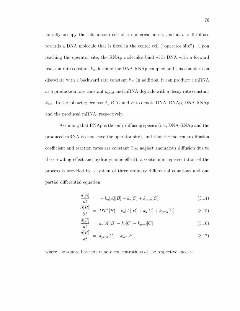
76
initially occupy the left-bottom cell of a numerical mesh, and at t > 0 diffuse
towards a DNA molecule that is fixed in the center cell (“operator site”). Upon
reaching the operator site, the RNAp molecules bind with DNA with a forward
reaction rate constant ka, forming the DNA-RNAp complex and this complex can
dissociate with a backward rate constant kd. In addition, it can produce a mRNA
at a production rate constant kprod and mRNA degrade with a decay rate constant
kdec. In the following, we use A, B, C and P to denote DNA, RNAp, DNA-RNAp
and the produced mRNA, respectively.
Assuming that RNAp is the only diffusing species (i.e., DNA-RNAp and the
produced mRNA do not leave the operator site), and that the molecular diffusion
coefficient and reaction rates are constant (i.e, neglect anomalous diffusion due to
the crowding effect and hydrodynamic effect), a continuum representation of the
process is provided by a system of three ordinary differential equations and one
partial differential equation,
d[A]
dt= − ka[A][B] + kd[C] + kprod[C] (3.14)
∂[B]
∂t= D∇2[B]− ka[A][B] + kd[C] + kprod[C] (3.15)
d[C]
dt= ka[A][B]− kd[C]− kprod[C] (3.16)
d[P ]
dt= kprod[C]− kdec[P ], (3.17)
where the square brackets denote concentrations of the respective species.

77
Reaction- vs. diffusion-limited processes
We set the molecular diffusion coefficient to D = 10−12 m2/s. Then the
average time for RNAp molecules to arrive at the operator site is 0.04 s, i.e.,
RNAp molecules diffuse quickly throughout the system that becomes “well-mixed”.
Diffusion does not have a significant impact on the system’s dynamics since the
system is reaction-controlled. In other words, D = 10−12 m2/s can result in a
reaction-limited (reaction-controlled) system.
Let us define a dimensionless Damkohler number Da as the ratio of typical
diffusion (τD) and reaction (τR) time scales,
Da =τDτR. (3.18)
A system is diffusion-limited if Da 1 and reaction-limited otherwise. For D =
10−12 m2/s, the average diffusion time τD ∈ [10−2 s, 10−1 s]. Since τR is of the
same order of magnitude, the system is reaction-limited. On the other hand, the
diffusion coefficient D = 10−15 m2/s corresponds to Da ∼ 103, resulting in the
diffusion-limited behavior.
Fig. 3.7A demonstrates the salient features of these two transport regimes
with L = 5. For D = 10−12 m2/s, the number of protein molecules computed with
the Gillespie algorithm (a perfectly mixed system with no diffusion) and with our
operator-splitting algorithm are in close agreement. For D = 10−15 m2/s, diffusion
becomes important with the protein beginning to burst around 20 s after the RNAp
molecules encounter DNA at the central operator site. Our results differ from their

78
counterparts obtained by the Gillespie algorithm mainly in terms of fluctuations.
Time-step selection
The magnitude of the molecular diffusion coefficient D affects the choice of
the time-step ∆t in the stochastic operator-splitting algorithm. Fig. 3.7A and 3.7B
show the number of mRNA molecules computed for a wide range of the diffusion
coefficients, 10−15 ≤ D ≤ 10−12 with L = 5 and L = 20, respectively. In the
case study with L = 5 and D = 10−12 m2/s, the time scales are τR = 0.012 s and
τD = 6×10⁻³ s; fast diffusion quickly homogenizes the system so that its behavior
is reaction-controlled. Our numerical experiments suggest that setting ∆t = 10τD
decreases the simulation time and guarantees that a reasonable number of reactions
take place during the simulation time-step.
For small diffusion coefficients (D = 10−15 m2/s), τD = 6.67 s and τR =
0.012 s, which means that almost all τR < τD. To ensure that a sufficient number
of reactions take place during the time interval ∆t, we selected ∆t = 2τD. Similar
rules are applied for L = 20 as well.
Comparison with GMP method and stochastic effect
The mRNA production, predicted with the GMP algorithm and our ap-
proach on the meshes with several degrees of refinement (L = 5, 10, 20), are shown
in Fig. 3.8A and B, respectively. In a display of the lack of self-consistency, the
finest mesh (L = 20) results in predictions that are quantitatively wrong in that

79
the system fails to reach its equilibrium state of about 1,000 proteins. It is worth-
while recalling that in the GMP algorithm, ∆t is defined as the minimal diffusion
time that cannot be adjusted. In the system under consideration, τR > ∆t so that
all the reactions cannot take place during the time interval ∆t (τR = 0.65 s and
τD = 0.417 s). These results demonstrate one of the advantages of our algorithm:
unlike the GMP algorithm, our approach is capable of handling different mesh
sizes by adapting appropriate time-steps.
The effects of stochasticity (noise) become apparent in predictions averaged
over a smaller number of realizations (Fig. 3.8C). As should be expected from the
central limit theorem, the standard deviation from the mean prediction decreases
as 1/√Nr. By ignoring the spatial variability, the Gillespie algorithm dampens
considerably the noise present in the system. The protein production continues to
fluctuate in time even after it reaches its equilibrium (steady-state) value because
it depends on the frequency of the encounter of RANp and DNA in the central
cell. The statistics of the equilibrium protein production, i.e., its mean µ, standard
deviation σ, and noise level (coefficient of variation) ν = σ/µ, are presented in
Table 3.6.

80
3.3.3 CheY diffusion case study
System description
As a final example, we consider a chemotaxis pathway in E. coli. A mathe-
matical model of this process has been developed earlier [73]. The species included
in the model [73] and their simplified spatial arrangement within a cell are pre-
sented in Table 3.8 and Fig. 3.9A, respectively. Table 3.7 lists a set of reactions
considered in this model. The diffusing species are CheY, CheYp and CheZ. The
species CheA∗ (active CheA) and CheAp do not diffuse into the cytoplasm, be-
ing confined in the inner receptor cluster. The molecules of CheY and CheA∗
are phosphorylated in the receptor cluster located on the anterior cell wall. Once
diffused into the cytoplasm, the CheYp molecules bind with four flagellar motors
FliM1,. . .,FliM4 and the FliM·CheYp complex is produced. The four motors are lo-
cated on the side walls, ordered FliM1 to FliM4 from the anterior wall (Fig. 3.9A).
The reactions in the FliMs induce E. coli’s forward or backward motion and/or
rotation.
The diffusion step in our stochastic operator-splitting algorithm is imple-
mented in a way that the molecules reaching the cell’s surface are reflected back
into the cell without loss of momentum. The diffusion step is followed by the re-
action step, which employs the Gillespie algorithm to simulate reactions between
the molecules within each cell of a numerical mesh. We investigate the effects of
varying the length of cell, Lsv (sv denotes subvolume) and time-step ∆t on the
81
performance of our algorithm, and compare it to that of the GMP algorithm.
Both GMP and our approach are conceptually different from the Smoldyn
method [73]. The latter approach simulates diffusion with Brownian dynamics
and keeps track of individual molecules. Unlike our algorithm, it allows for multi-
molecular reactions between two or three molecules only within a certain radius
from each other. This reduces the computational speed and increases storage
requirements, because positions of all molecules have to be stored and distances
between all molecules must be calculated at each step in order to check if reactions
can take place.
Simulation results
The time-course of FliM·CheYp complexes simulated with both the GMP
algorithm and our stochastic operator-splitting approach is shown in Figs. 3.9B,
C. The GMP algorithm overestimates the equilibrium levels of the FliM·CheYp
complexes and underestimates the transition-to-equilibrium times in both Fig. 3.9B
(M1 and M2) and Fig. 3.9C (M3 and M4). As established in the two previous
computational examples, this discrepancy is due to the errors associated with the
cellular automaton treatment of diffusion in the GMP algorithm. In addition to
being more accurate, our approach is also computationally more efficient than the
GMP algorithm. In both algorithms, the reaction step consumes close to 99% of the
total computational time. Therefore, in order to reduce the simulation time, larger
∆t should be selected because the execution of the Gillespie algorithm accounts

82
for most of the computational time. For a given mesh size Lsv, the time-step in
the GMP algorithm is fixed by the molecular diffusion coefficient D, while in our
algorithm it is more flexible according to whether the system is reaction-controlled
or diffusion-controlled. The simulation time for our algorithm is 12hrs, whereas it
is 26 hrs for the GMP method.
3.4 Summary and Discussion
Complex multi-scale biological systems can be analyzed with microscopic
approaches, such as Greens-function reaction dynamics and the Smoldyn algo-
rithm. These methods are accurate albeit computationally expensive and often
prohibitive. On the other hand, macroscopic kinetic modeling approaches that
use PDEs are amenable to numerical computation, but fail to model the physics
of systems with small number of molecules accurately. Mesoscopic approaches,
e.g., reaction-diffusion master equation and MesoRD, discretize space into a col-
lection of lattice elements and extend the chemical master equation normally used
in well-mixed chemical reactions into the stochastic regime for inhomogeneous sys-
tems. To facilitate faster and more accurate solutions within the mesoscopic scale
framework, we have developed a stochastic simulation method which is based on
operator-splitting for modeling the reaction-diffusion system. In our methodology,
the time-step size is chosen automatically at each step depending upon whether
the system is reaction- or diffusion-controlled. We use the Gillespie stochastic sim-

83
ulation algorithm for modeling the reactions and Brownian dynamics approach for
modeling the diffusion process. We thus account for both spatial heterogeneity
and the fluctuation in concentrations arising from the small number of molecules.
Our method yields highly accurate results and has the merit of modeling both the
reaction and diffusion processes in the system.
In order to validate accuracy and efficiency of our algorithm, a simple
reaction-diffusion system, A+B → C, is studied first. We concluded that Brownian
dynamics provides much more accurate results while being faster than a Cellular
automata approach. For example, Table 3.3 reveals that the error-rates for our
approach and the GMP algorithm are about 1% and 5%, respectively. The average
speed-up by using our method is about 5 times as compared to the GMP method
for a wide range of the values of the diffusion constant. Moreover, we compared
the stochastic ensemble average with the deterministic result and found out that
our results converge to the deterministic result when smaller ∆t and larger L are
used in the simulation. We also concluded that the fluctuations become larger in
case of smaller number of molecules and spatial inhomogeneity.
Towards modeling biologically realistic systems, a simplified gene expres-
sion system and CheY diffusion in E. coli bacteria are studied. In gene expression
case study, the system is classified based on the Damkohler number, Da. If it
is larger than 1, it is regarded as a diffusion-limited system and reaction-limited
otherwise. In order to simulate the system accurately, the time-step, ∆t, should
be selected according to the dominant process. In addition, noise levels concerning
84
the number of molecules and number of realizations are studied. It is shown that as
the number of molecules or number of realizations become smaller, the noise level
increases. We then simulated a more complicated system, viz., CheY diffusion in
E. Coli, through both the GMP method and our operator-splitting algorithm. We
have shown that the operator-splitting approach provides more accurate results
and is faster as compared to the GMP algorithm. For a more accurate analysis of
movement of E. coli bacteria, the chemotaxis process in which molecules move to-
ward higher or lower concentration according to the concentration gradient should
also be analyzed [78].
In conclusion, we present a hybrid numerical method, also known as, operator-
splitting method, for stochastic reaction-diffusion process with a small number of
heterogeneously distributed molecules. Our approach is conceptually similar to
the GMP algorithm that applies Gillespie algorithm for reaction process and Cel-
lular automata for diffusion process. However, our method provides computational
advantages in terms of accuracy and efficiency. First, molecules in Brownian dy-
namics can move freely without the restriction of lattice or time-step whereas
molecules in Cellular automata move only to the adjacent lattices during the fixed
time-step. Second, Brownian dynamics offers a more accurate simulation result
than the cellular automata approach. Third, our algorithm has the flexibility of
changing time-steps, depending on whether the system is reaction- or diffusion-
controlled.

85
TaiJung Choi, Mano R. Maurya, Daniel M. Tartakovsky, Shankar Subra-
maniam (2012), ‘Stochastic Operator-Splitting Method for Reaction-Diffusion Sys-
tems’. J. Chem. Phys., 137, 184102
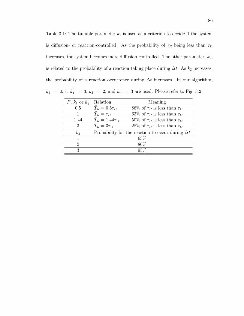
86
Table 3.1: The tunable parameter k1 is used as a criterion to decide if the system
is diffusion- or reaction-controlled. As the probability of τR being less than τD
increases, the system becomes more diffusion-controlled. The other parameter, k2,
is related to the probability of a reaction taking place during ∆t. As k2 increases,
the probability of a reaction occurrence during ∆t increases. In our algorithm,
k1 = 0.5 , k′1 = 3, k2 = 2, and k
′2 = 3 are used. Please refer to Fig. 3.2.
F , k1 or k′1 Relation Meaning
0.5 TR = 0.5τD 86% of τR is less than τD1 TR = τD 63% of τR is less than τD
1.44 TR = 1.44τD 50% of τR is less than τD3 TR = 3τD 28% of τR is less than τD
k2 Probability for the reaction to occur during ∆t1 63%2 86%3 95%
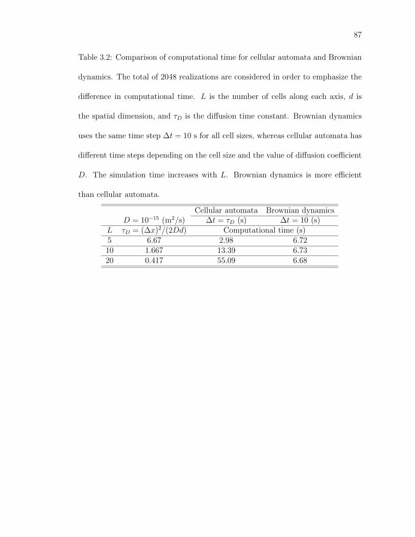
87
Table 3.2: Comparison of computational time for cellular automata and Brownian
dynamics. The total of 2048 realizations are considered in order to emphasize the
difference in computational time. L is the number of cells along each axis, d is
the spatial dimension, and τD is the diffusion time constant. Brownian dynamics
uses the same time step ∆t = 10 s for all cell sizes, whereas cellular automata has
different time steps depending on the cell size and the value of diffusion coefficient
D. The simulation time increases with L. Brownian dynamics is more efficient
than cellular automata.
Cellular automata Brownian dynamicsD = 10−15 (m2/s) ∆t = τD (s) ∆t = 10 (s)
L τD = (∆x)2/(2Dd) Computational time (s)5 6.67 2.98 6.7210 1.667 13.39 6.7320 0.417 55.09 6.68
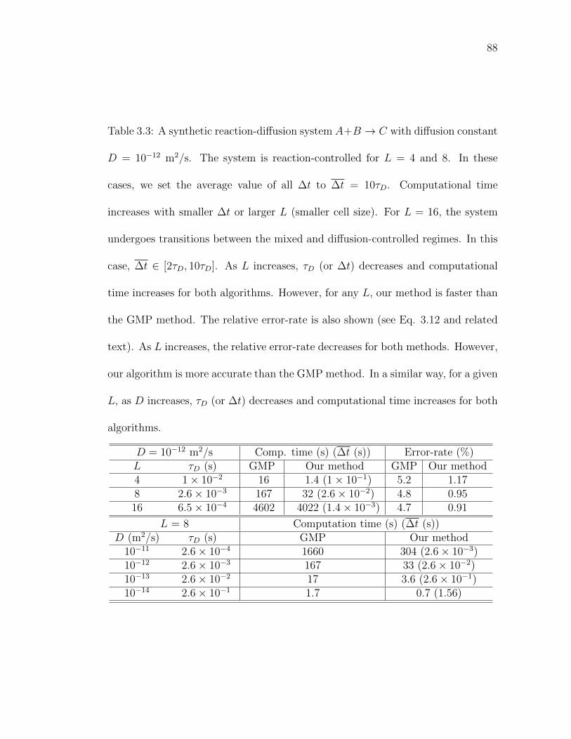
88
Table 3.3: A synthetic reaction-diffusion system A+B → C with diffusion constant
D = 10−12 m2/s. The system is reaction-controlled for L = 4 and 8. In these
cases, we set the average value of all ∆t to ∆t = 10τD. Computational time
increases with smaller ∆t or larger L (smaller cell size). For L = 16, the system
undergoes transitions between the mixed and diffusion-controlled regimes. In this
case, ∆t ∈ [2τD, 10τD]. As L increases, τD (or ∆t) decreases and computational
time increases for both algorithms. However, for any L, our method is faster than
the GMP method. The relative error-rate is also shown (see Eq. 3.12 and related
text). As L increases, the relative error-rate decreases for both methods. However,
our algorithm is more accurate than the GMP method. In a similar way, for a given
L, as D increases, τD (or ∆t) decreases and computational time increases for both
algorithms.
D = 10−12 m2/s Comp. time (s) (∆t (s)) Error-rate (%)L τD (s) GMP Our method GMP Our method4 1× 10⁻² 16 1.4 (1× 10⁻¹) 5.2 1.178 2.6× 10⁻³ 167 32 (2.6× 10⁻²) 4.8 0.9516 6.5× 10⁻⁴ 4602 4022 (1.4× 10⁻³) 4.7 0.91
L = 8 Computation time (s) (∆t (s))D (m2/s) τD (s) GMP Our method
10−11 2.6× 10⁻⁴ 1660 304 (2.6× 10⁻³)10−12 2.6× 10⁻³ 167 33 (2.6× 10⁻²)10−13 2.6× 10⁻² 17 3.6 (2.6× 10⁻¹)10−14 2.6× 10⁻¹ 1.7 0.7 (1.56)

89
Table 3.4: Gene expression case study: DNA has 1 molecule and RNAp has 18
molecules. C is the DNA·RNAp complex. System volume is 1×10⁻¹⁵ l and diffusion
coefficient of RNAp is D = 10−12 m2/s (reaction-limited system) or D = 10−15
m2/s (diffusion-limited system). Abbreviation: I.C.: initial condition.
Reaction Rate I.C. [nM]
DNA + RNApka−→ C 3× 10⁹ M−1s−1 1.67
Ckd−→ DNA +RNAp 21.5 s−1 30
Ckprod−−−→ P + DNA + RNAp 89.55 s−1 0
Pkdec−−→ φ 0.04 s−1 0

90
Table 3.5: Gene expression case study: Reaction time is averaged over 256 realiza-
tions of a simplified gene expression process. As cell sizes become smaller reaction
times increase, since fewer molecules in each cell imply lower probability for reac-
tions to take place within a cell. The time-step ∆t in the GMP method equals
τD, whereas ∆t in our method can vary according to the system classification as
reaction- or diffusion-controlled. Since the cases of L = 5 and 10 are diffusion-
controlled, we set ∆t = 2τD. For L = 20, the system changes from diffusion- to
reaction-controlled as time progresses.
D = 10−15 m2/s GMP Our method
L ∆x (µm) τR τD = ∆x2
2Dd(s) ∆t (s)
5 0.2 0.012 6.67 13.3310 0.1 0.095 1.667 3.3320 0.05 0.65 0.417 2.34
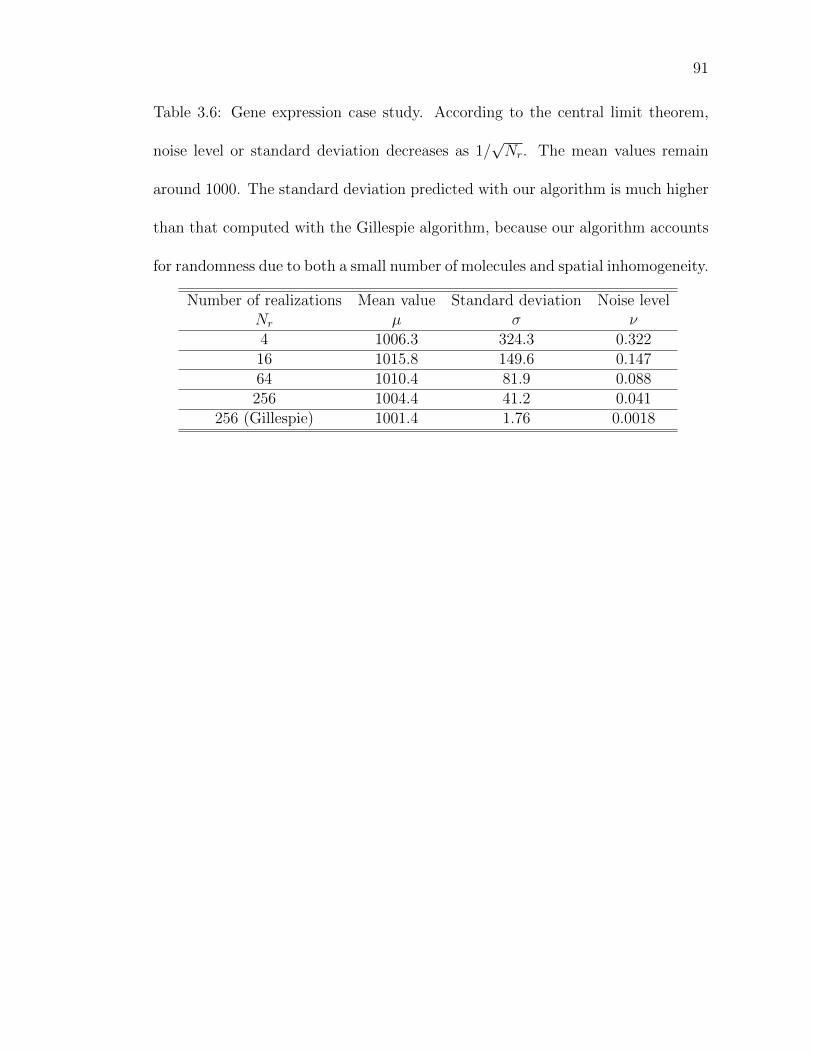
91
Table 3.6: Gene expression case study. According to the central limit theorem,
noise level or standard deviation decreases as 1/√Nr. The mean values remain
around 1000. The standard deviation predicted with our algorithm is much higher
than that computed with the Gillespie algorithm, because our algorithm accounts
for randomness due to both a small number of molecules and spatial inhomogeneity.
Number of realizations Mean value Standard deviation Noise levelNr µ σ ν4 1006.3 324.3 0.32216 1015.8 149.6 0.14764 1010.4 81.9 0.088256 1004.4 41.2 0.041
256 (Gillespie) 1001.4 1.76 0.0018

92
Table 3.7: CheY diffusion case study: kf and kb denote respectively forward and
backward reaction rate constants for the E. coli system. Unimolecular and bimolec-
ular reaction rates have dimensions [s−1] and [M−1s−1], respectively. i denotes the
index of flagellar motors.
Compartment Reaction Reaction constant
Receptor clusterCheA∗ → CheAp kf = 3.4× 101 s−1
CheAp+CheY → CheA∗+CheYp kf = 108 M−1s−1
CytoplasmCheY CheYp
kf = 5.0× 10⁻⁵ s−1
kb = 8.5× 10⁻² s−1
CheZ+CheYp → CheZ+CheY kf = 1.6× 10⁶ M−1s−1
FliMi (i = 1, . . . , 4) FliMi+CheYp FliMi·CheYpkf = 5.0× 10⁶ M−1s−1
kb = 2.0× 101 s−1
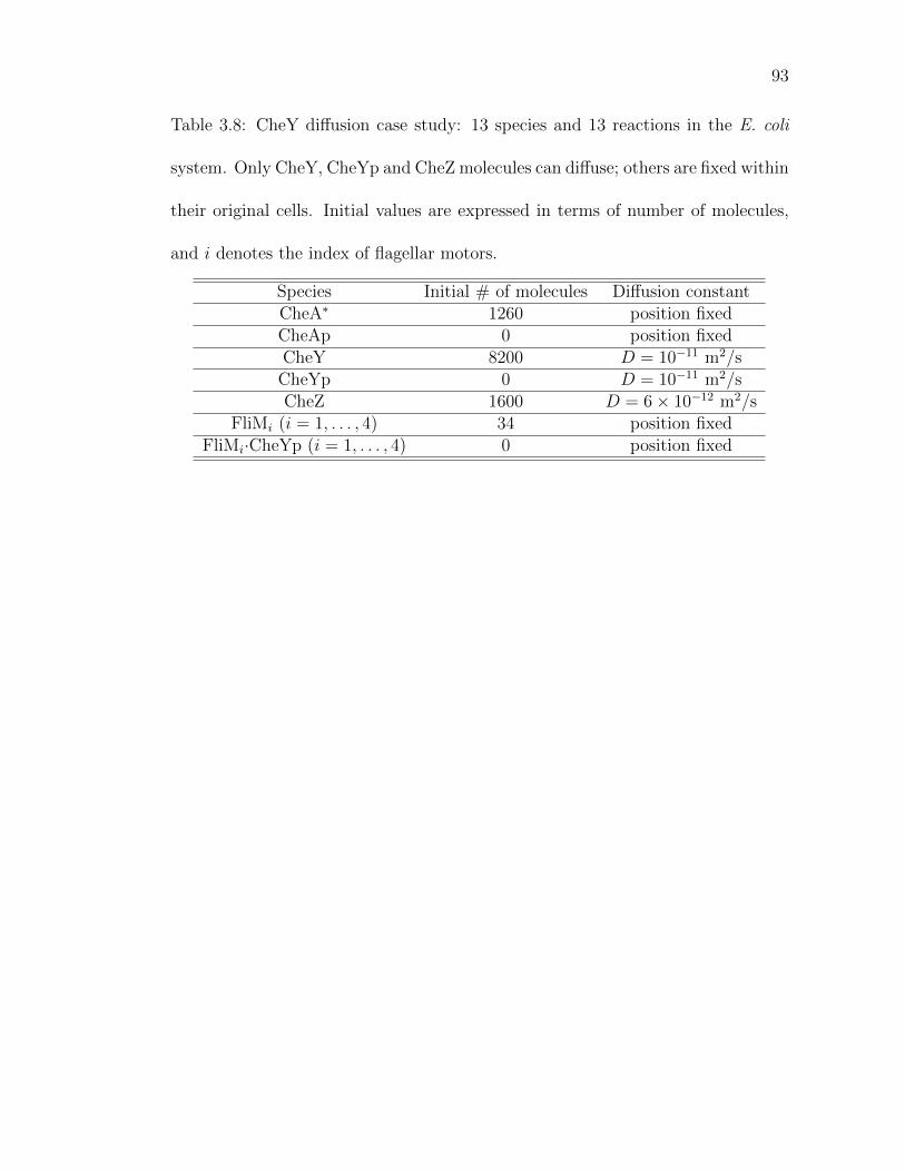
93
Table 3.8: CheY diffusion case study: 13 species and 13 reactions in the E. coli
system. Only CheY, CheYp and CheZ molecules can diffuse; others are fixed within
their original cells. Initial values are expressed in terms of number of molecules,
and i denotes the index of flagellar motors.
Species Initial # of molecules Diffusion constantCheA∗ 1260 position fixedCheAp 0 position fixedCheY 8200 D = 10−11 m2/s
CheYp 0 D = 10−11 m2/sCheZ 1600 D = 6× 10⁻¹² m2/s
FliMi (i = 1, . . . , 4) 34 position fixedFliMi·CheYp (i = 1, . . . , 4) 0 position fixed

94
Diffusion
Reaction
c(x, t) c(x, t)
c(x, t)
∆t
∆t
c(x, t)
≡ c(x, t + ∆t)
(A)
(B) (C)
C E
N
W
S
C E
N
W
S
NE
SESW
NW
Diffusion
Reaction
c(x, t) c(x, t)
c(x, t)
∆t
∆t
c(x, t)
≡ c(x, t + ∆t)
(A)
(B) (C)
Figure 3.1: (A) Schematic representation of the diffusion-reaction operator-
splitting. The final value after diffusion process at time t + ∆t is used as the
initial value for the reaction process. Final value of reaction process is the final
value at the end of diffusion-reaction process. (B)-(C) Cellular automata neigh-
borhoods in d = 2 dimension: in the von Neumann automata the probability of
staying in a cell or diffusing to its neighbors is 1/5 (B), in the Moore automata
this probability is 1/9 (C).
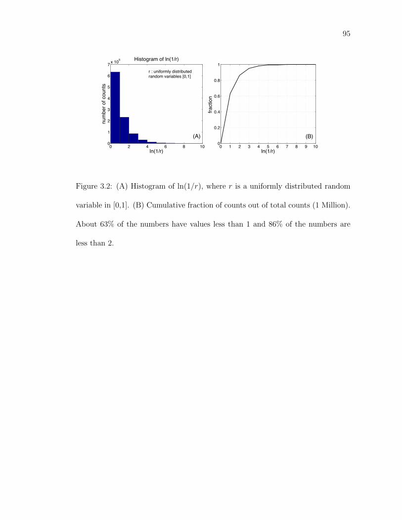
95
0 2 4 6 8 100
1
2
3
4
5
6
7 x 10⁵
ln(1/r)
num
ber o
f cou
nts
Histogram of ln(1/r)
0 1 2 3 4 5 6 7 8 9 100
0.2
0.4
0.6
0.8
1
ln(1/r)
fract
ion
(A) (B)
r : uniformly distributed random variables [0,1]
Figure 3.2: (A) Histogram of ln(1/r), where r is a uniformly distributed random
variable in [0,1]. (B) Cumulative fraction of counts out of total counts (1 Million).
About 63% of the numbers have values less than 1 and 86% of the numbers are
less than 2.
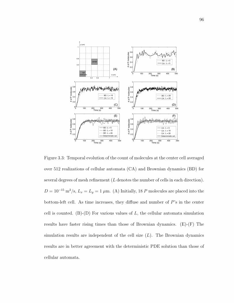
96
0 100 200 300 400 5000
0.2
0.4
0.6
0.8
1
Time (s)
# of
P m
olec
ules
0 100 200 300 400 5000
0.2
0.4
0.6
0.8
1
Time (s)
# of
P m
olec
ules
B.D: L = 5B.D: L = 10B.D: L = 20Deterministic sol.
C.A: L = 5C.A: L = 10C.A: L = 20Deterministic sol.
0 100 200 300 400 5000
0.2
0.4
0.6
0.8
1
Time (s)
# of
P m
olec
ules
B.D: L = 5C.A: L = 5
0 100 200 300 400 5000
0.2
0.4
0.6
0.8
1
Time (s)
# of
P m
olec
ules
B.D: L = 10C.A: L = 10
0 100 200 300 400 5000
0.2
0.4
0.6
0.8
1
Time (s)
# of
P m
olec
ules
B.D: L = 20C.A: L = 20
(B)
(D)
(F)
center
y (um)
x (um)
0.4 0.6
0.4
0.6
1
1
18 Pmolecules
(A)
(C)
(E)
(A)
0 100 200 300 400 5000
0.2
0.4
0.6
0.8
1
Time (s)
Mea
n: #
of P
mol
ecul
es
B.D: Ln = 5B.D: Ln = 10B.D: Ln = 20
0 100 200 300 400 5000
0.2
0.4
0.6
0.8
1
Time (s)
Mea
n: #
of P
mol
ecul
es
C.A: Ln = 5C.A: Ln = 10C.A: Ln = 20
0 100 200 300 400 5000
0.2
0.4
0.6
0.8
1
Time (s)
Mea
n: #
of P
mol
ecul
es
B.D: Ln = 5C.A: Ln = 5
0 100 200 300 400 5000
0.2
0.4
0.6
0.8
1
Time (s)
Mea
n: #
of P
mol
ecul
es
B.D: Ln = 10C.A: Ln = 10
0 100 200 300 400 5000
0.2
0.4
0.6
0.8
1
Time (s)
Mea
n: #
of P
mol
ecul
es
B.D: Ln = 20C.A: Ln = 20
(B)
(D)
(F)
(C)
(E)
(A)
L=10L=10
L=20L=20
L=5L=10L=20
L=5L=10L=20
0 100 200 300 400 5000
0.2
0.4
0.6
0.8
1
Time (s)
Mea
n: #
of P
mol
ecul
es
B.D: Ln = 5C.A: Ln = 5
0 100 200 300 400 5000
0.2
0.4
0.6
0.8
1
Time (s)M
ean:
# o
f P m
olec
ules
B.D: Ln = 10C.A: Ln = 10
0 100 200 300 400 5000
0.2
0.4
0.6
0.8
1
Time (s)
Mea
n: #
of P
mol
ecul
es
B.D: Ln = 20C.A: Ln = 20
L=5L=5
1
1
y (um)
x (um)
0.6
0.4
0.4 0.6
center
18Pmolecules
(A)
BDCA
BDCA
BDCA
BDBDBD
CACACA
Figure 3.3: Temporal evolution of the count of molecules at the center cell averaged
over 512 realizations of cellular automata (CA) and Brownian dynamics (BD) for
several degrees of mesh refinement (L denotes the number of cells in each direction).
D = 10−15 m2/s, Lx = Ly = 1 µm. (A) Initially, 18 P molecules are placed into the
bottom-left cell. As time increases, they diffuse and number of P ’s in the center
cell is counted. (B)-(D) For various values of L, the cellular automata simulation
results have faster rising times than those of Brownian dynamics. (E)-(F) The
simulation results are independent of the cell size (L). The Brownian dynamics
results are in better agreement with the deterministic PDE solution than those of
cellular automata.

97
Figure 3.4: A + B → C case study: (A) Initially, species A and B exist only in
left-hand side. All A and B molecules and their product P diffuse with the same
diffusion constant. (B) Comparison of results from analytical solution, cellular
automata (CA) and Brownian dynamics (BD). The Brownian dynamics results
agree with the analytical solution, while the cellular automata results do not. The
increasing curves represent the number of molecules in the right half of the domain
and the decreasing ones in the left half.

98
10 14 10 13 10 12 10 1110 4
10 2
100
102
Diffusion constant (D)
! D(o
r!
t)(s
)
GMPOur method
10 14 10 13 10 12 10 1110 1
100
101
102
103
104
Diffusion constant (D)Co
mpu
tatio
n tim
e (s
)
GMPOur method
(B)(A)
Figure 3.5: A+B → C case study: Effect of diffusion constant, D (m2/s), on (A)
τD (or ∆t) and (B) computational time for our method and the GMP method.
As D increases, τD (or ∆t) decreases and computational time increases for both
algorithms. For D = 10−14 m2/s, the system transitions from diffusion-controlled
(∆t = k2τD; k2 = 2) to reaction-controlled regime during the time-course. For
D ≥ 10−13 m2/s, the system becomes reaction-controlled (∆t = 10τD), explaining
the increase in the absolute value of the slope of ∆t or computational time vs. D
plots at D = 10−13 m2/s for our method.
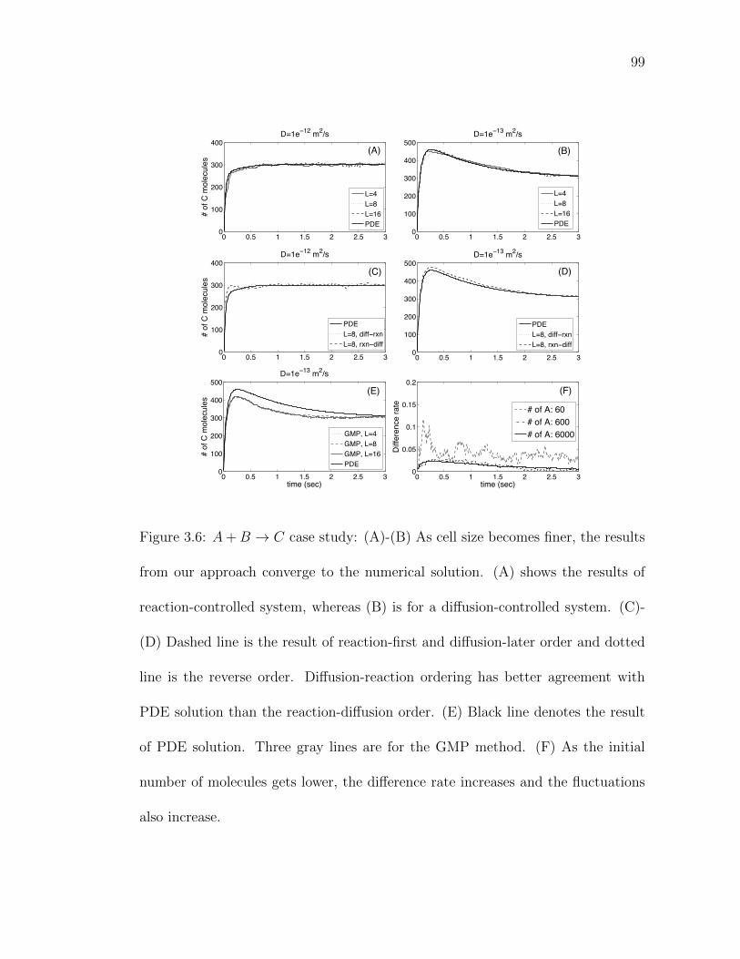
99
0 0.5 1 1.5 2 2.5 30
100
200
300
400D=1e 12 m2/s
# of
C m
olec
ules
L=4L=8L=16PDE
0 0.5 1 1.5 2 2.5 30
100
200
300
400
500D=1e 13 m2/s
L=4L=8L=16PDE
0 0.5 1 1.5 2 2.5 30
100
200
300
400D=1e 12 m2/s
# of
C m
olec
ules
0 0.5 1 1.5 2 2.5 30
100
200
300
400
500D=1e 13 m2/s
PDEL=8, diff rxnL=8, rxn diff
0 0.5 1 1.5 2 2.5 30
100
200
300
400
500D=1e 13 m2/s
time (sec)
# of
C m
olec
ules
GMP, L=4GMP, L=8GMP, L=16PDE
PDEL=8, diff rxnL=8, rxn diff
0 0.5 1 1.5 2 2.5 30
0.05
0.1
0.15
0.2
time (sec)
Diff
eren
ce ra
te
# of A: 60# of A: 600# of A: 6000
(C)
(B)
(D)
(A)
(E) (F)
Figure 3.6: A+B → C case study: (A)-(B) As cell size becomes finer, the results
from our approach converge to the numerical solution. (A) shows the results of
reaction-controlled system, whereas (B) is for a diffusion-controlled system. (C)-
(D) Dashed line is the result of reaction-first and diffusion-later order and dotted
line is the reverse order. Diffusion-reaction ordering has better agreement with
PDE solution than the reaction-diffusion order. (E) Black line denotes the result
of PDE solution. Three gray lines are for the GMP method. (F) As the initial
number of molecules gets lower, the difference rate increases and the fluctuations
also increase.

100
0 100 200 300 400 5000
200
400
600
800
1000
1200L=5
# of
P m
olec
ules
D=1e 12D=1e 13D=1e 14D=1e 15Gillespie
0 100 200 300 400 5000
200
400
600
800
1000
1200L=20
time (sec)
# of
P m
olec
ules
D=1e 12D=1e 13D=1e 14D=1e 15
(B)
(A)
Figure 3.7: Gene expression case study: (A) Dash-dotted line shows the result
of Gillespie algorithm which deals with only reaction process. For D = 10−12
m2/s with L = 5, our results are similar to those obtained with the Gillespie
algorithm, because it is a reaction-limited process so that diffusion does not have
serious impact on the system. On the contrary, the case of D = 10−15 m2/s with
L = 5 exhibits long time lag to reach the steady-state value due to diffusion effect
and has much larger fluctuations. (B) In case of L = 20, the mesh is much finer
than the above cases. The results are similar to those in (A) as our algorithm is
able to adjust time-steps according to the system characteristics even though L is
increased from 5 to 20.

101
0 100 200 300 400 5000
200
400
600
800
1000
1200GMP
# o
f P m
olec
ules
L=5L=10L=20
0 100 200 300 400 5000
200
400
600
800
1000
1200Our method
# of
P m
olec
ules
L=5L=10L=20
0 1000 2000 3000 4000 50000
500
1000
1500
2000
Fluctuation level
time (sec)
# of
P m
olec
ules
256 runs64 runs16 runs4 runsGillespie(256 runs)
(A)
(B)
(C)
Figure 3.8: Gene expression case study: (A) The result of GMP algorithm for
various L and the corresponding ∆t (= τD) values. Diffusion constant has a
fixed value, D = 10−15 m2/s. For L = 20 (τR = 0.65 s and τD = 0.417 s),
the number of P molecules does not reach its steady-state value of around 1000
because τR > ∆t = τD (Table 3.5). This means reactions cannot fully take place
during ∆t. (B) Our algorithm performs well for both cases of L because it classifies
the system as diffusion- or reaction-controlled and decides the appropriate time-
steps accordingly. (C) Fluctuations become smaller as the number of realizations
become larger. In comparison to the Gillespie algorithm, our method has much
higher fluctuations because it considers spatial randomness as well as randomness
due to the small number of molecules.
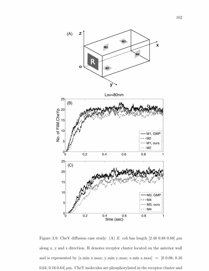
102
(A)
M2
M3
M1
M4
0 0.2 0.4 0.6 0.8 10
5
10
15
20
25Lsv=80nm
No.
of F
liM.C
heYp
M1, GMPM2M1, oursM2
0 0.2 0.4 0.6 0.8 10
5
10
15
20
25
time (sec)
M3, GMPM4M3, oursM4
(B)
(C)
Figure 3.9: CheY diffusion case study: (A) E. coli has length [2.48 0.88 0.88] µm
along x, y and z direction. R denotes receptor cluster located on the anterior wall
and is represented by [x min x max; y min y max; z min z max] = [0 0.08; 0.16
0.64; 0.16 0.64] µm. CheY molecules are phosphorylated in the receptor cluster and
diffuse into the cytoplasm. M1∼M4 show the location of the four flagellar motors
on side walls and are located in M1 = [0.48 0.56; 0.40 0.48; 0 0.08] µm, M2
= [0.96 1.04; 0 0.08; 0.40 0.48] µm, M3 = [1.44 1.52; 0.40 0.48; 0.80 0.88] µm and
M4 = [1.92 2.00; 0.80 0.88; 0.40 0.48] µm. The remaining domain is considered
as cytoplasm. (B)-(C) The simulation results from both the GMP method and
our method are in good agreement although there are some differences in rise-time
because the GMP method and our method use cellular automata and Brownian
dynamics, respectively, to model the diffusion process (as explained in Fig. 3.4).

Chapter 4
Stochastic Models of
Chemotaxis-Diffusion-Reaction
Processes in Wound Healing
4.1 Introduction
Complexity of biochemical systems is manifested through the presence of
multiple species, reactions and processes, and of multiple spatial and temporal
scales. Cells respond to stimulus by activating myriad biochemical networks, al-
tering the cellular state and ending up in an altered phenotype. In the context of
inflammation-mediated immune response, the early cellular signaling events occur
103

104
in seconds to minutes, leading to a complex cascade of spatially- and temporally-
correlated events that culminate in the final immune response after a few days.
Traditional approaches model immune responses or other biological processes at
each temporal or spatial scale. For instance, molecular simulations deal with the
movement of atoms in proteins on the milliseconds time scale, kinetic modeling of
reaction networks models processes on the time scales of seconds to hours, while
heuristic models of biological systems capture processes that occur on the time
scale of days. We rely on some of the recent advances in computational methods
and power, and in acquisition and assimilation of data across multiple scales in
biological systems, to develop and apply novel multi-scale simulation algorithms
to model leukocyte movement during inflammation and wound healing.
Leukocytes respond to skin or tissue injury through an inflammation process
that involves their adhesion and rolling along endothelium cells, transmigration and
chemotaxis. The movement and physiology of leukocytes after transmigrations
are governed by three processes: chemotaxis, diffusion and chemical reactions.
Chemotaxis is represented by an advection term in advection-diffusion-reaction
equations. Its strength depends on the concentration gradient of chemoattractants
that are released from an injury site.
Deterministic ordinary differential equations (ODEs) often provide accurate
predictions of the dynamics of biochemical pathways (complex reaction chains with
large numbers of reacting molecules). However, they fail when concentrations of
reactants and/or their products become small and the law of mass action be-

105
comes invalid. Under these conditions, randomness in the dynamics of individual
molecules becomes pronounced and requires stochastic simulations. Stochasticity
plays a critical role in the behavior of many micro-scale biological phenomena, such
as cellular signaling and gene regulatory networks [8, 70, 71]. Standard stochastic
techniques, e.g., the Gillespie stochastic simulation algorithm [11] and its compu-
tationally efficient modifications [12, 70, 72], can be used to model biochemical
reactions in such systems. These algorithms are applicable to systems in which
reactants and their products are distributed uniformly in space.
Spatial inhomogeneity has to be considered in crowded environments with
complex internal geometry. If the number of molecules is large, partial differen-
tial equations (PDEs) provide accurate macroscopic predictions of the dynamics of
spatially distributed systems. However, similar to ODE-based models, determin-
istic PDEs fail to predict random events in systems comprised of small numbers
of molecules. Computational methods for reaction-diffusion systems with small
numbers of molecules must be able to handle both stochasticity and heterogeneity.
Our stochastic numerical algorithm [79] described in Chapter 3 employs an oper-
ator splitting, in which the Gillespie algorithm (or its accelerated versions) and
Brownian dynamics (or the Smoluchowski equation) are used to model reactions
and diffusion, respectively. It employs adaptive time steps to handle both reaction-
controlled and diffusion-controlled systems. To model inflammation processes, we
enhance this algorithm by incorporating another spatial effect due to chemotaxis.
Four phases of wound healing are briefly discussed in Section 4.2. Our

106
mathematical model of inflammation is described in Section 4.3. It is followed by
introduction of a stochastic operator-splitting approach in Section 4.4. This section
also contains a brief description of our stochastic simulation algorithm for modeling
reactions and chemotaxis-diffusion. Sections 4.5 and 4.6 contain simulation results
and conclusions, respectively.
4.2 Wound healing
Wound healing is a complicated process of tissue repair after injury or
damage. It is divided into four sequential but overlapping phases: hemostasis,
inflammation, proliferation, and remodeling [80].
4.2.1 Hemostasis
Upon injury in the tissue, a cascade of biochemical events takes place to
repair the damage. Within few minutes after injury, in order to control bleeding,
platelets aggregate at the injury site to form a fibrin clot. Next, vasoconstric-
tion is followed by vasodilation that causes blood vessels to become porous by
releasing histamine. Increased porosity of blood vessels facilitates transmigration
of leukocytes from bloodstream to the wound site.

107
4.2.2 Inflammation
Within an hour of wounding, polymorphonuclear neutrophils (PMNs) arrive
at the wound site to phagocytize debris and kill bacteria [80]. As fewer inflamma-
tory factors are secreted, numbers of neutrophils and macrophages are reduced at
the wound site and inflammation process ends. However, if the inflammatory phase
lasts for too long, e.g., due to the presence of dirt or other foreign objects, it could
lead to a chronic wound [81]. This inflammation process includes the leukocytes
movement through rolling, adhesion, transmigration and chemotaxis ([82] and Fig.
4.1).
From rolling to chemotaxis
A leukocyte adhesion cascade during the inflammatory phase consists of
rolling, firm adhesion and transmigration. Each of these steps plays an impor-
tant role in effective leukocyte recruitment to the damaged tissues. Rolling, which
is mediated by selectin family (L-, P-, E-selectins), is characterized by leukocyte
movement with a typical velocity of approximately 5 ∼ 10 µm/s and rolling dis-
tance on the order of 100 µm. Adhesion, which is facilitated by integrins and their
binding molecules, is a much slower process characterized by a velocity on the
order of v = 10 µm/min and crawled distance on the order of 10 µm [83]. After
firm adhesion, leukocytes transmigrate (with a certain probability) into the tissue
through the endothelium cells whose thickness is about 1 ∼ 2 µm. Once in the
tissue, leukocytes move toward a wound area driven by diffusion and chemotaxis.

108
All these processes have a wide range of time- and length-scales, which makes it
necessary to develop a multi-scale modeling framework.
Capture and rolling
The first contact of a leukocyte with the activated endothelium is referred to
as “capture” or “tethering”. Once leukocytes are captured, they may adhere to the
endothelium and begin to roll. It is common to refer to a leukocyte as rolling when
its rolling velocity is less than half of the blood stream velocity. This process is
mediated by the selectin family (L-, E-, P-selectins), and transitory bonds between
selectins and their ligands are formed and broken during the rolling motion [82].
Firm adhesion
E-selectin participates in the conversion of rolling to firm adhesion. This
process is facilitated by integrins (LFA-1, Mac-1, VLA-4), which are activated
by chemokines and soluble factors released by endothelial cells. In the activated
state, integrins bind tightly to corresponding receptors expressed on endothelial
cells. As a result, despite the shear force of blood flow, the leukocytes are nearly
immobilized [82].
Transmigration
After firm adhesion, leukocytes migrate to a wound area in the tissue by
extending pseudopodia and passing either through gaps between endothelial cells

109
(paracellular) or directly through the cells (transcellular) [84]. Paracellular trans-
migration is not well understood. It is thought that they migrate out of blood ves-
sels in a homophilic way, assisted by bindings of VE-cadherin, PECAM-1, CD99
and JAM family molecules [85] found on the leukocyte and endothelial cell surfaces.
Chemotaxis
After transmigrating from blood vessels, leukocyte cells (neutrophils arrive
first) move along the concentration gradient of chemicals (chemokines or cytokines,
e.g., fMLP or N-formyl-methionine-leucine-phenylalanine) that are produced at
and diffused from the wound site. Chemotaxis causes leukocytes to migrate prefer-
entially in the concentration gradient direction with some probability called chemo-
tactic index (CI). (In addition to chemotaxis, leukocytes also diffuse down their
concentration’s gradient.)
4.2.3 Proliferation
The proliferative phase is represented by angiogenesis, collagen deposition,
tissue formation and epithelialization [81]. During proliferation, the wound is re-
built with new granulation tissue that is comprised of collagen and extracellular
matrix. The process known as angiogenesis leads to development of a new network
of blood vessels and healthy granulation tissue. Its efficacy depends on the fibrob-
last receiving sufficient levels of oxygen and nutrients supplied by blood vessels.
Epithelial cells resurface the wound, a process known as epithelialization.
110
4.2.4 Remodeling
The remodeling phase can last several months or even years. During this
phase, collagen is remodeled and complete wound contraction takes place. Wound
strength increases from about 20% to 80% within 3 weeks to two years after in-
jury [86].
4.3 A mathematical model of inflammation
Let b(x, t), a(x, t) and c(x, t) denote the concentrations of bacteria, attrac-
tant and leukocyte, respectively. Under certain assumptions, these concentrations
change due to the mechanisms that are described by the following equations [87].
• Bacteria diffuse, reproduce, and are destroyed when they come in contact
with leukocytes:
∂b
∂t= µb∇2b+ (kg − kdc)b, (4.1)
where µb and kg are respectively the diffusion coefficient and growth rate of
bacteria. This formulation assumes linear kinetics of the bacteria consump-
tion by leukocytes, with the consumption rate kd.
• The chemoattractant is produced by bacterial metabolism and diffuses:
∂a
∂t= D∇2a+ kpb, (4.2)
where D and kp are the diffusion coefficient and production rate of the
chemoattractant, respectively.
111
• The leukocytes are chemotactically attracted to the attractant and die when
they digest the bacteria:
∂c
∂t= −∇ · Jc − (g0 + g1b)c, Jc = −µ∇c+ χc∇a. (4.3)
Here the reaction term represents linear kinetics of leukocytes destruction due
to both natural death in the tissue (with rate constant g0) and interactions
with bacteria (with rate constant g1, which we set to g1 = kd in the subsequent
analysis). The equilibrium flux of leukocytes, Jc, is parameterized by the
diffusion coefficient of leukocytes µ and the chemotaxis coefficient χ.
4.3.1 Diffusion
Chemoattractant and bacteria diffusion
We treat diffusion of chemoattractant and bacteria as continuous processes
that are governed by diffusion equations. These are solved by finite differences to
yield the concentrations of chemoattractant and bacteria, b(x, t) and a(x, t). The
concentration of chemoattractant affects chemotaxis of leukocytes, such that leuko-
cytes move towards the wound site where the concentration of chemoattractant is
highest.
Leukocyte diffusion
Motility of a cell population, i.e., diffusion of leukocytes, is described by
the motility coefficient (diffusion coefficient) µ. Random motility of a single cell
112
is characterized by its speed v and persistence time Tp. The latter is defined as
the time interval during which a cell moves without changing direction [88]. The
population and single-particle motility coefficients are related by [7]
µ =1
2Tpv
2, v = |v|. (4.4)
4.3.2 Chemotaxis
At the continuum level, chemotactic velocity Vc is the product of “oriental
bias” φ and macroscopic leukocyte velocity v =∑
i viei [88],
Vc =∑i
φiviei =∑i
χi∂a
∂xi. (4.5)
Since the oriental bias is defined by [88]
φi =χ0dNb
da
∂a
∂xi
1 + χ0dNb
da
∂a
∂xi
, (4.6)
the chemotaxis coefficient has the form
χi = viχ0dNb
da
1 + χ0dNb
da
∂a
∂xi
ei, (4.7)
where i(= 1, 2 and 3) is the number of dimensions.
The constant χ0 is called chemotactic sensitivity and 0 ≤ φ ≤ 1, such
that φ = 0 represents purely random process and φ = 1 corresponds to perfectly
directed motion. A Michaelis-Menten relationship
Nb =NTa
Kd + a(4.8)

113
is used to relate the number of bound receptors on the cell membrane, Nb, to the
concentration of attractant, a [87]. Here Kd is the receptor dissociation constant,
and NT is the total number of cell receptors on the cell membrane.
4.3.3 Reactions
We assume that bacteria and leukocyte have negligible volume. Bacteria
(B) reproduce with the rate kg, leukocytes (C) die with the rate g0, and bacteria
and leukocytes react and die with reaction rate kd or g1.
Bkg−→ 2B, C
g0−→ φ B + Ckd(=g1)−−−−→ φ. (4.9)
The reaction constant kd is defined as [?]
kd = 4π(µB + µ)(rB + rC), (4.10)
where µb and µ are the diffusion constant of bacteria and leukocytes and r is the
radius. We set kd = g1, since it is assumed that both bacteria and leukocytes
die when they enter the same neighborhood of radius rB + rC . In the simulations
reported below we set rB = 1 µm and rC = 10 µm. Values of the other model
parameters (reaction rates, diffusion coefficients, and chemotactic constant) are
listed in Table 4.1.
114
4.4 Numerical approach
We extend our stochastic operator splitting approach [79] (Chapter 3), in
which reactions are handled through a stochastic simulation algorithm (e.g., Gille-
spie’s [11]) and diffusion is treated through Brownian dynamics. Leukocytes moves
through chemotaxis and diffusion. Bacteria and leukocytes undergo biochemical
reactions. Spatio-temporal evolution of leukocytes concentrations can be described
by a system of chemotaxis-diffusion-reaction equations,
∂c
∂t+∇ · (Vcc) = µ∇2c− (g0 + g1b)c (4.11)
where Vc is the chemotactic velocity vector and µ is diffusion coefficient and re-
actions terms are explained in Eq. 4.3.
We employ an operator-splitting algorithm to approximate Eq. 4.11 with
∂c′
∂t= µ∇2c′ −∇ · (Vcc
′) (4.12a)
∂c′′
∂t= −(g0 + g1b)c
′′. (4.12b)
during the time interval [t, t+ ∆t]. Here c′(t) = c(t) and c′′(t) = c′(t+ ∆t), so that
the concentration of leukocytes at the end of the time-step ∆t is c′′(t) = c(t+ ∆t).
115
4.5 Simulation results
4.5.1 Chemotaxis and diffusion
Brian and his colleagues conducted many experiments and showed how
chemotaxis, chemokinesis and diffusion affect the movement of leukocytes [88] .
Based on the same concept, we start simulations by modeling leukocyte movement
without considering the reactions involved. To focus on the interplay between the
chemoattractant concentration and the leukocyte movement, we solve only (4.2)
and (4.3).
Since the diffusion coefficient of the chemoattractant is much higher than
that of leukocytes (D µ), the chemoattractant diffuses through the tissue much
faster than leukocytes move. Moreover, the number of chemoattractant molecules
is large enough to ignore stochastic fluctuations in their movement and to warrant
the reliance on the deterministic diffusion equation (4.2). Its deterministic solution
is to be coupled with the stochastic simulations of the leukocytes movement.
One-dimensional migration
To be concrete, we take the simulation domain to be Ω = [xs, xe] = [0, 2×
10−3] m, and impose the following initial and boundary conditions
I.C.s : a(x, 0) = 0, c(xe2, 0) = c0, (4.13a)
B.C.s : a(xe, t) = a0,∂a
∂x|xs,xe = 0,
∂c
∂x|xs,xe = 0, (4.13b)

116
where a0 is 1 × 10⁻⁹ M and c0 is 10000, the initial number of leukocytes. Here,
reaction term kpb is considered as a source at x = xe and has a value of a0. Stochas-
tic simulations of leukocyte migration replace the deterministic (one-dimensional)
chemotaxis-diffusion equation (4.3) with its stochastic counterpart
X(t+ ∆t) = X(t) + Vc∆t+√
2µ∆tξ (4.14)
where ∆t is the time step, Vc is computed from the one-dimensional versions of (4.5)
and (4.7) and ξ is a standard Gaussian random variable.
In Fig. 4.2, we study the effect as strength of chemotaxis increases and all
plots are captured at t = 10000 sec. Initially, ten thousands of leukocytes exist
in the middle of the x axis and source of chemoattractant exists at the end of x
axis. In case that there exists only diffusion process, blue-colored line looks to be
normally distributed. When weak chemotaxis process (χ0) is added to the system,
plot moves to the right, which means more leukocytes moves to the right where
concentration of chemoattractant is higher. As chemotactic sensitivity increases,
chemotactic index, φ, increases. Accordingly, larger number of leukocytes moves
toward chemoattractant source point as chemotactic sensitivity increases.
Two-dimensional migration
Consider leukocyte migration in a two-dimensional domain Ω = [xs, xe] ×
[ys, ye]. The two-dimensional versions of (4.2) and (4.3) are subject to initial and
117
boundary conditions
I.C.s : a(x, y, 0) = 0, c(0.4xe, 0.1ye, 0) = c0, (4.15a)
B.C.s : a(xe2, ys, t) = a0,
∂a
∂x|xs,xe =
∂a
∂y|ys,ye = 0, (4.15b)
∂c
∂x|xs,xe =
∂c
∂y|ys,ye = 0, (4.15c)
where [xs, xe] = [ys, ye] = [0, 4×10⁻³] m and a0 is 1×10⁻⁸ M and c0 is 3, the initial
number of leukocytes. We use the alternating direction implicit (ADI) method [74]
to solve the deterministic two-dimensional equation (4.2). The ADI method solves
two one-dimensional problems at each time step:
an+1/2ij − anijD∆t/2
=an+1/2i+1j − 2a
n+1/2ij + a
n+1/2i−1j
∆x2+anij+1 − 2anij + anij−1
∆y2(4.16a)
an+1ij − an+1/2
ij
D∆t/2=an+1/2i+1j − 2a
n+1/2ij + a
n+1/2i−1j
∆x2+an+1ij+1 − 2an+1
ij + an+1ij−1
∆y2. (4.16b)
The reaction term, kpb, can be thought as a source term in the wound site.
Leukocyte displacements in the x and y directions are computed stochastically
with (4.14).
Figure 4.3 shows the geometry and the simulation results for leukocyte
movement. Leukocyte movement due to chemotaxis increases as chemotaxis con-
stant increases in the same manner as 1D simulation. At t = 5000 sec, leukocytes
with stronger chemotaxis (10χ0) arrive at the wound site, meanwhile those with
weaker chemotaxis (χ0) are still moving forward to wound site.
118
4.5.2 Chemotaxis, diffusion and reactions
In this section, reactions are considered as well as chemotaxis and diffu-
sion. We employ operator splitting algorithm explained in Sec. 3.2.1. Leukocyte
migration can be characterized by (dimensionless) Peclet number
Pe =Vch
D=τDτC
(4.17)
where h is the mesh (or lattice) size, and τD and τC are diffusion and convection
time scales, respectively. If Pe > 1, chemotaxis is slower than diffusion. Since
this regime is dominated by diffusion, we designate τD as the drift time constant.
Inversely, if Pe < 1, τC is chosen as the drift time constant. Finally, we define
Damkohler number as
Da =min(τC , τD)
τR(4.18)
The value of the Damkohler number determines whether the system is drift con-
trolled or reaction controlled in the operator splitting algorithm [79].
Figure 4.4 shows the three-dimensional geometry of the simulation domain,
Ω = [xs, xe]× [ys, ye]× [zs, ze].
I.C.s : a(x, y, z, 0) = 0, c(x, y, z, 0) = c0, (4.19a)
B.C.s : a(xe2, ys, zs, t) = a0,
∂a
∂x|xs,xe =
∂a
∂y|ys,ye =
∂a
∂z|zs,ze = 0, (4.19b)
∂c
∂x|xs,xe =
∂c
∂y|ys,ye =
∂c
∂z|zs,ze = 0, (4.19c)
where [xs, xe] = [ys, ye] = [zs, ze] = [0, 1×10⁻³] m and a0 is 1×10⁻⁸ M and c0 is 500,
the initial number of leukocytes which are positioned arbitrarily inside the domain,

119
Ω. Chemoattractant diffusion is solved by the three-dimensional ADI method in
the same method as 3D ADI. Leukocytes diffuse randomly and chemotax in the
system. Bacteria are fixed in the small rectangle and can react with leukocytes
when they meet in the same mesh.
In Table 4.2, we can see that chemotactic index increases as strength of
chemotaxis increases. As a result, more bacteria are digested through more fre-
quent reactions. However, the change of random motility have no significant effect
upon the number of bacteria. It means that chemotaxis sensitivity has a stronger
effect to inflammation than diffusion (random motility).
4.6 Summary and Discussion
We apply stochastic operator splitting method to inflammation process dur-
ing wound healing. Mathematical modeling is described by partial differential
equations comprised of chemotaxis, diffusion and reaction processes. It is very
difficult and improper to employ deterministic approach due to a wide variety
of temporal and spatial scales. Therefore, we analyze chemoattractant diffusion
equation using deterministic ADI method because molecular diffusion is much
faster than leukocytes and bacteria and number of chemoattractant molecules is
reasonably high. However, leukocytes movement and reactions with bacteria are
analyzed stochastically by operator splitting algorithm. We consider Peclet and
Damkoler number in order to decide drift time scale and if system is diffusion or
120
drift controlled.
In order to verify if simulation works properly, diffusion and chemotaxis are
studied first without reaction in 1D and 2D. We figure out that more leukocytes
move forward to wound site as chemotactic constant increase. Next, reactions are
analyzed with drift in 3D simulation. Similarly, more leukocytes move to wound
site as chemotactic constant increases. As a result, more reactions take place and
more bacteria are digested by leukocytes.

121
Table 4.1: Constants for reaction, diffusion and chemotaxis.
Notation Description Value [Unit]χ0 chemotactic sensitivity 4e−8 [m/receptor]µb random motility coeff. of bacteria 0µ random motility coeff. of leukocytes calculated in Eq. 4.4 [m2/s]D diffusion constant of chemoattractants 1e−9 [m2/s]kg generation rate of bacteria 1.4e−4 [s−1]
kd(= g1) decay rate of bacteria/leukocytes calculated in Eq. 4.10 [M−1s−1]kp production rate of bacteria - [s−1]g0 generation rate of leukocytes 2e−6 [s−1]

122
Table 4.2: Initial number of bacteria and leukocytes are 50 and 500. 32 simula-
tions are conducted for 10000 sec. As chemotactic constant increases, chemotactic
index increases, which means more leukocytes move forward to wound site. As
a result, more reactions take place and more bacteria are killed. However, the
change of random motility have no significant effect upon the number of bacte-
ria. It means that chemotaxis has a stronger effect to inflammation than diffusion
(random motility).
Strength of chemotaxis Chemotactic index Mean of number of bacteria100χ0 0.4 ∼ 0.5 3.510χ0 0.3 ∼ 0.4 26.5χ0 ∼ 0.05 48.8
Random motility coeff. Chemotactic index Mean of number of bacteria10µ ∼ 0.05 48.11µ ∼ 0.05 48.8
0.1µ ∼ 0.05 50

123
Figure 4.1: Leukocytes flow along the blood stream. When injury occurs in the
tissue, they begin to roll and adhere on endothelium cells. Next, they transmigrate
through endothelial cells by the effect of histamine. Transmigrated leukocytes move
toward lesions by chemotaxis and diffusion processes.
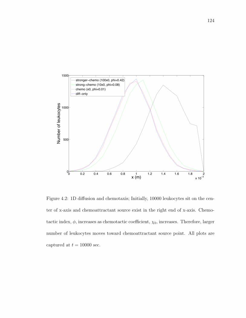
124
0 0.2 0.4 0.6 0.8 1 1.2 1.4 1.6 1.8 2x 10 3
0
500
1000
1500
x (m)
Num
ber o
f leu
kocy
tes
stronger chemo (100x0, phi=0.42)strong chemo (10x0, phi=0.08)chemo (x0, phi=0.01)diff only
Figure 4.2: 1D diffusion and chemotaxis; Initially, 10000 leukocytes sit on the cen-
ter of x-axis and chemoattractant source exist in the right end of x-axis. Chemo-
tactic index, φ, increases as chemotactic coefficient, χ0, increases. Therefore, larger
number of leukocytes moves toward chemoattractant source point. All plots are
captured at t = 10000 sec.

125
0 1 2 3 4x 10 3
0
0.5
1
1.5
2
2.5
3
3.5
4 x 10 3
x (m)
y (m
)
0 1 2 3 4x 10 3
0
0.5
1
1.5
2
2.5
3
3.5
4 x 10 3
x (m)
y (m
)
t = 5000 sec, 0
0 1 2 3 4x 10 3
0
0.5
1
1.5
2
2.5
3
3.5
4 x 10 3
x (m)
y (m
)
t = 5000 sec, 10 0
0.02
0.03
0.04
0.05
0.06
0.07
0.08
0.09
0.1
Chemoattractant concentration (x10 7M)
Figure 4.3: 2D diffusion and chemotaxis; (A) It shows the concentration distri-
bution of chemoattractant. The center of x axis is the source point. (B)-(C)
Leukocytes moves toward chemoattractant source point as chemotactic coefficient
increases. The positions of leukocytes are traced from t = 0 to 5000 sec. The color
is changed from red (t = 0 → 1667 sec) to green (t = 1667 → 3333 sec) and to
blue (t = 3333→ 5000 sec) as simulation time increases.

126
Bacteria
Leukocytes
Source/B.C
Figure 4.4: 3D diffusion, chemotaxis and reactions; Leukocytes diffuse randomly
in the whole domain. Bacteria are fixed in small cube and considered as a source
of chemoattractant in the center of x axis.

Chapter 5
Conclusions
This dissertation leads to the following major conclusions:
1. We have developed a hybrid approach to stochastic simulation, in which slow
reactions and fluxes are handled through exact stochastic simulation and their
fast counterparts are treated partially deterministically through the chemical
Langevin equation. The classification of reactions as fast or slow is accompa-
nied by a partial equilibrium assumption, according to which a population of
slow species is not altered by fast reactions. Our new approach also handles
reactions with complex rate expressions such as functions of Michaelis-Menten
kinetics and power-law kinetics by developing mathematical expressions for
their propensity functions and microscopic fluxes. Fluxes which cannot be
modeled explicitly through reactions are handled deterministically.
2. We have integrated the existing techniques for multiscale stochastic simula-
127

128
tion with deterministic simulation to deal with complex reactions systems and
have applied it to studying calcium dynamics in macrophage cells. When the
concentration of reactants is sufficiently large, the stochastic method yields
time-course profiles identical to those obtained from a deterministic model
(ensemble average of 16 or more realizations). However, at lower number of
molecules of one or more species, measurable relative difference in [Ca2+]i re-
sponses predicted by the two approaches is obtained, especially for the case of
Gβγ, thus suggesting the necessity of using stochastic simulation as opposed to
deterministic simulation for studying system dynamics at sub-cellular levels.
Dose response analysis revealed that while the normalized response difference
(NRD) between [Ca2+]i responses predicted by deterministic and stochastic
simulations is negligible at the full dose of 30nM (shown) or higher doses
including saturating doses (not shown), it increases with decreasing doses.
At 0.1% dose, it is as high as 7%. These results are emphasized again in
the sensitivity analysis of the parameters used in the simulation and in the
knockdown analysis of reacting protein components.
3. Complex multi-scale biological systems can be analyzed with microscopic ap-
proaches, such as Green’s-function reaction dynamics and the Smoldyn algo-
rithm. These methods are accurate albeit computationally expensive and of-
ten prohibitive. On the other hand, macroscopic kinetic modeling approaches
that use PDEs are amenable to numerical computation, but fail to model the
physics of systems with small number of molecules accurately. Mesoscopic
129
approaches, e.g., reaction-diffusion master equation and MesoRD, discretize
space into a collection of lattice elements and extend the chemical master
equation normally used in well-mixed chemical reactions into the stochastic
regime for inhomogeneous systems. To facilitate faster and more accurate so-
lutions within the mesoscopic scale framework, we have developed a stochas-
tic simulation method which is based on operator-splitting for modeling the
reaction-diffusion system. In our methodology, the time-step size is chosen
automatically at each step depending upon whether the system is reaction-
or diffusion-controlled. We use the Gillespie stochastic simulation algorithm
for modeling the reactions and Brownian dynamics approach for modeling
the diffusion process. We thus account for both spatial heterogeneity and the
fluctuation in concentrations arising from the small number of molecules. Our
method yields highly accurate results and has the merit of modeling both the
reaction and diffusion processes in the system. We also have a better result
in terms of simulation speed over GMP method. The average speed-up by
using our method is about 5 times as compared to the GMP method for a
wide range of the values of the diffusion constant in case of simple reaction-
diffusion system, A + B → C. In more complicated system, CheY diffusion
in E. coli, the simulation time for our algorithm is 12hrs, whereas it is 26 hrs
for the GMP method.
4. We applied stochastic operator splitting method to inflammation process dur-
ing wound healing. The mathematical modeling is described by partial differ-

130
ential equations comprised of chemotaxis, diffusion and reaction processes. It
is difficult and improper to employ deterministic approach due to a wide vari-
ety of temporal and spatial scales. Therefore, we analyze chemoattractant dif-
fusion equation using deterministic ADI method because molecular diffusion
is much faster than leukocytes and bacteria and number of chemoattractant
molecules is reasonably high. However, leukocyte movement and reactions
with bacteria are analyzed stochastically by operator splitting algorithm. We
consider Peclet and Damkoler number in order to decide drift time scale and
if system is diffusion- or drift- controlled. In the studies on diffusion and
chemotaxis in 1D and 2D, we figure out that more leukocytes move forward
to wound site as chemotactic constant increase. In 3D simulation with drift
and reactions, more leukocytes move to wound site as chemotactic constant
increases and thus more reactions take place and more bacteria are digested
by leukocytes.

Appendix A
Existing algorithms for stochastic
simulation
Three algorithms, namely Gillespie algorithm, tau-leap method and chemi-
cal Langevin equation are reviewed. These algorithms are applied to a well-stirred
biochemical system (molecules of each species are spread uniformly throughout
a fixed control volume) at thermal equilibrium comprising M different chemical
reactions and N different types of chemical species.
At any time t, the population of molecules within a fixed cellular volume
V is uniquely described by a state vector X(t),
X(t) = X1(t), X2(t), . . . , XN(t)T , (A.1)
where Xi(t) is the number of molecules of the i-th species (i = 1, . . . , N). By
definition, Xi are non-negative integers. The state vector X(t) changes whenever
131
132
one of the M types of reactions occur.
Let P [X; t] denote the probability of the system being in the state rep-
resented in Eq. (A.1) at time t. Furthermore, let aj(X) denote the propensity
function of the j-th reaction channel, which is defined through aj(X)dt, the prob-
ability that the j-th reaction will occur during a (sufficiently small) time interval
[t, t + dt] given the system state X(t) at time t. The propensity function aj(X)
can be expressed as [61]
aj(X) = cjhj(X), j ∈M, M = 1, 2, . . . ,M, (A.2a)
where cj > 0 is the specific probability rate constant of the j-th reaction, and
hj(X) is the number of possible combinations of reactants in the j-th reaction.
The former is given by
cj =
kj for monomolecular reactions
2kjNAV
for bimolecular reactions with identical reactants
kjNAV
for bimolecular reactions with different reactants
(A.2b)
where NA = 6.022× 10²³ mol−1 is Avogadro’s constant, and kj is the macroscopic
133
reaction rate constant [89]. The latter has the form
hj(X) =
1 for reactions of type: φ→ product(s) [no reactants]
Xi for monomolecular reactions [A→ B]
Xi(Xi − 1)/2 for reactions with identical reactants [A+ A→ C]
XiXk for reactions with different reactants [A+B → C]
(A.2c)
for some 1 ≤ j ≤M , and 1 ≤ i, k ≤ N with i 6= k.
Let the time-interval dt in the definition of aj(X) (Eq. (A.2)) be small
enough that at most one reaction occurs during [t, t+ dt), then P [X; t] satisfies an
ODE that is commonly called a chemical master equation (CME) [61],
dP [X; t]
dt=
M∑j=1
aj(X− νj)P [X− νj; t]− aj(X)P [X; t], (A.3)
where νj = (νj1 , . . . , νjN )T is a vector whose entries are the numbers of molecules
of each species added to or removed from the volume V due to the j-th reaction.
For complex cellular processes, such as calcium dynamics in the signaling network
described in Section 2.3.1, high-dimensionality of the CME (Eq. (A.3)) renders
its solutions computationally prohibitive. The standard simulation algorithms de-
scribed below serve to overcome the computational burden associated with solving
Eq. (A.3).
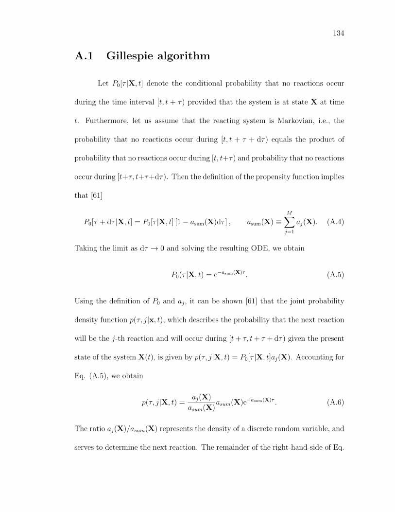
134
A.1 Gillespie algorithm
Let P0[τ |X, t] denote the conditional probability that no reactions occur
during the time interval [t, t + τ) provided that the system is at state X at time
t. Furthermore, let us assume that the reacting system is Markovian, i.e., the
probability that no reactions occur during [t, t + τ + dτ) equals the product of
probability that no reactions occur during [t, t+τ) and probability that no reactions
occur during [t+τ, t+τ+dτ). Then the definition of the propensity function implies
that [61]
P0[τ + dτ |X, t] = P0[τ |X, t] [1− asum(X)dτ ] , asum(X) ≡M∑j=1
aj(X). (A.4)
Taking the limit as dτ → 0 and solving the resulting ODE, we obtain
P0(τ |X, t) = e−asum(X)τ . (A.5)
Using the definition of P0 and aj, it can be shown [61] that the joint probability
density function p(τ, j|x, t), which describes the probability that the next reaction
will be the j-th reaction and will occur during [t+ τ, t+ τ + dτ) given the present
state of the system X(t), is given by p(τ, j|X, t) = P0[τ |X, t]aj(X). Accounting for
Eq. (A.5), we obtain
p(τ, j|X, t) =aj(X)
asum(X)asum(X)e−asum(X)τ . (A.6)
The ratio aj(X)/asum(X) represents the density of a discrete random variable, and
serves to determine the next reaction. The remainder of the right-hand-side of Eq.

135
(A.6), asum(X) exp[−asum(X)τ ] is the exponential density function of a continuous
random variable, which corresponds to the time at which the next reaction will
occur.
To advance the system from state X(t), the Gillespie algorithm generates
two random variables r1 and r2 distributed uniformly on the unit interval [0, 1].
According to Eq. (A.6), a discrete random value j and continuous random value
τ are selected as
τ =1
asum
ln
(1
r1
),
j−1∑j′=1
aj′ ≤ r2asum ≤j∑
j′=1
aj′ . (A.7)
The system is then updated according to X(t+ τ) = X(t) + νj.
A faster algorithm for exact stochastic simulation has been presented by
[64], called ”next reaction method”. This approach is about an order of magni-
tude faster than the Gillespie algorithm discussed above.However, this approach
does not scale as well as the tau-leap algorithm discussed below as the number of
molecules increases.
A.2 Tau-leap algorithm
The tau-leap algorithm [12] can be used to increase the computational effi-
ciency of the Gillespie algorithm when it is used to simulate large reactive systems
consisting of many reactions and molecules. This algorithm allows many reactions
to take place simultaneously during a time interval [t, t+τ). Let Kj(τ |X, t) denote
the number of times j-th reaction (1 ≤ j ≤M) takes place during the time inter-
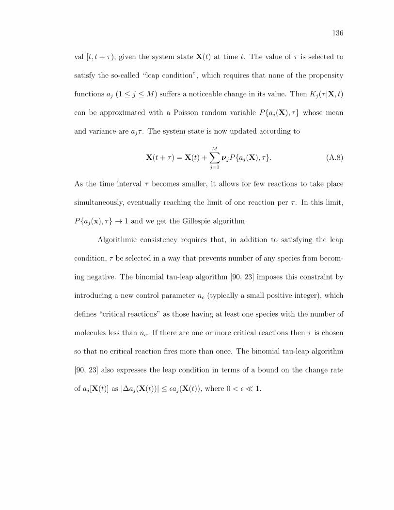
136
val [t, t + τ), given the system state X(t) at time t. The value of τ is selected to
satisfy the so-called “leap condition”, which requires that none of the propensity
functions aj (1 ≤ j ≤M) suffers a noticeable change in its value. Then Kj(τ |X, t)
can be approximated with a Poisson random variable Paj(X), τ whose mean
and variance are ajτ . The system state is now updated according to
X(t+ τ) = X(t) +M∑j=1
νjPaj(X), τ. (A.8)
As the time interval τ becomes smaller, it allows for few reactions to take place
simultaneously, eventually reaching the limit of one reaction per τ . In this limit,
Paj(x), τ → 1 and we get the Gillespie algorithm.
Algorithmic consistency requires that, in addition to satisfying the leap
condition, τ be selected in a way that prevents number of any species from becom-
ing negative. The binomial tau-leap algorithm [90, 23] imposes this constraint by
introducing a new control parameter nc (typically a small positive integer), which
defines “critical reactions” as those having at least one species with the number of
molecules less than nc. If there are one or more critical reactions then τ is chosen
so that no critical reaction fires more than once. The binomial tau-leap algorithm
[90, 23] also expresses the leap condition in terms of a bound on the change rate
of aj[X(t)] as |∆aj(X(t))| ≤ εaj(X(t)), where 0 < ε 1.
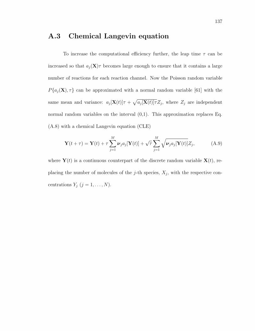
137
A.3 Chemical Langevin equation
To increase the computational efficiency further, the leap time τ can be
increased so that aj(X)τ becomes large enough to ensure that it contains a large
number of reactions for each reaction channel. Now the Poisson random variable
Paj(X), τ can be approximated with a normal random variable [61] with the
same mean and variance: aj[X(t)]τ +√aj[X(t)]τZj, where Zj are independent
normal random variables on the interval (0,1). This approximation replaces Eq.
(A.8) with a chemical Langevin equation (CLE)
Y(t+ τ) = Y(t) + τM∑j=1
νjaj[Y(t)] +√τ
M∑j=1
√νjaj[Y(t)]Zj, (A.9)
where Y(t) is a continuous counterpart of the discrete random variable X(t), re-
placing the number of molecules of the j-th species, Xj, with the respective con-
centrations Yj (j = 1, . . . , N).

Appendix B
Diffusion processes and GMP
algorithm
B.1 Diffusion process: Brownian dynamics
In cells, molecules such as proteins and metabolites, have a non-zero instan-
taneous speed at room temperature or at the temperature of the human body. A
typical protein molecule is immersed in the aqueous medium of a living cell. It col-
lides with other molecules in the solution, exhibiting a random walk or Brownian
motion.
Let X(t) ∈ R3 denote the position of a diffusing molecule at time t. Dif-
fusive spreading of molecules of the i-th species (i = 1, . . . ,M) is characterized
by a molecular diffusion coefficient Di, whose value depends on the molecule size,
absolute temperature and the viscosity of a solution. The molecule’s position at
138

139
the end of the time interval 4t is computed as follows [77].
1. Generate three normally distributed random numbers ξ1, ξ2, and ξ3 that serve
as components of the random displacement vector ξ = (ξ1, ξ2, ξ3)T .
2. Compute the molecule’s position at time t+4t as
X(t+4t) = X(t) +√
2Di4t ξ. (B.1)
3. Set t = t+4t and go to step 1.
B.2 Diffusion process: Cellular automata
In general, cellular automata depend on mesh size and diffusion constant.
Simulation accuracy and computational time vary according to neighborhood types [20].
For the two-dimensional example in Figs. 1B-C (main manuscript), molecules can
diffuse to four adjacent cells (voxel) or stay in the original voxel in the von Neu-
mann neighborhood, whereas in the Moore neighborhood they can diffuse to eight
adjacent cells or stay in the original voxel. If (0, 0) denotes the original voxel, the
von Neumann neighborhood is a set NN = (−1, 0), (0,−1), (0, 0), (0, 1), (1, 0).
The Moore neighborhood is a set NM = NN ∪ (−1,−1), (−1, 1), (1,−1), (1, 1).
The Gillespie multi-particle (GMP) algorithm [17] employs cellular au-
tomata to simulate diffusion. A diffusion-time constant τDi, the time during which
a molecule of the i-th species remains in one cell of a mesh, is given by [18]
τDi=
1
2d
(∆x)2
Di
, (B.2)

140
where Di is the diffusion coefficient for the i-th species. Moreover, a reaction-time
constant τR is defined as the ensemble average of the equivalent time constants for
all reactions related to diffusing molecules.
B.3 Gillespie multi-particle (GMP) method
We implemented the following GMP algorithm based on [18].
1. Set tS = ∆t = miniτDi for all diffusing species i.
2. Initialize t = 0 and ni = 1 for all diffusing species.
3. While t ≤ tfinal
• Reset tS = miniτDi· ni for all diffusing species.
• Reset told = t.
• For each cell, use the Gillespie algorithm to simulate reactions.
(a) While t ≤ tS
Calculate τR using Eq. 3.3.
– If t ≤ tS, find which reaction takes place within τR using Eq. 3.3.
Update number of species and time:
x← x + νj, t← t+ τR (B.3)
where νj is defined as the change of number of molecules.
– Else; do not update the state vector x since no reaction has occured.

141
end while
(b) Reset t = told for the next cell.
end for
• Use the cellular automata to diffuse the species.
• Reset ni ← ni + 1 for the diffused species.
• Set t = tS.
end while
Bibliography
[1] Erwin SCHRODINGER, What is Life?: With Mind and Matter and Autobi-ographical Sketches, Cambridge University Press, 1992.
[2] Michael B. Elowitz, Arnold J. Levine, Eric D. Siggia, and Peter S. Swain,“Stochastic gene expression in a single cell,” Science, vol. 297, no. 5584, pp.1183–1186, 08 2002.
[3] Harley H. McAdams and Adam Arkin, “Stochastic mechanisms in gene ex-pression,” Proceedings of the National Academy of Sciences, vol. 94, no. 3,pp. 814–819, 02 1997.
[4] Oleg Yarchuk, Nathalie Jacques, Jean Guillerez, and Marc Dreyfus, “Interde-pendence of translation, transcription and mrna degradation in the lacz gene,”Journal of Molecular Biology, vol. 226, no. 3, pp. 581–596, 8 1992.
[5] Yoon-Dong Yu, Yoonjoo Choi, Yik-Ying Teo, and Andrew R. Dalby, “Devel-oping stochastic models for spatial inference: Bacterial chemotaxis,” PLoSONE, vol. 5, no. 5, 05 2010.
[6] Gabriel Amselem, Matthias Theves, Albert Bae, Eberhard Bodenschatz,and Carsten Beta, “A stochastic description of ¡italic¿dictyostelium¡/italic¿chemotaxis,” PLoS ONE, vol. 7, no. 5, 05 2012.
[7] D. A. Lauffenburger, “Measurement of phenomenological parameters forleukocyte motility and chemotaxis.,” Agents Actions Suppl, vol. 12, pp. 34–53,1983.
[8] U. S. Bhalla, P. T. Ram, and R. Iyengar, “Map kinase phosphatase as alocus of flexibility in a mitogen-activated protein kinase signaling network,”Science, vol. 297, no. 5583, pp. 1018–1023, 2002.
[9] M. R. Maurya and S. Subramaniam, “A kinetic model for calcium dynamics inraw 264.7 cells: 1. mechanisms, parameters, and subpopulational variability,”Biophysical Journal, vol. 93, pp. 709–728, 2007.
[10] Jurgen Pahle Ursula Kummer, Borut Krajnc, Anne K. Green, C. Jane Dixon,and Marko Marhl, “Transition from stochastic to deterministic behavior incalcium oscillations,” Biophysical Journal, vol. 89, pp. 1603–1611, 2005.
142
143
[11] Daniel T. Gillespie, “Exact stochastic simulation of coupled chemical reac-tions,” The Journal of Physical Chemistry, vol. 81, no. 25, pp. 2340–2361, 121977.
[12] Yang Cao, Daniel T. Gillespie, and Linda R. Petzold, “Efficient step sizeselection for the tau-leaping simulation method,” The Journal of ChemicalPhysics, vol. 124, no. 4, pp. 044109–11, 01 2006.
[13] Vassilios Sotiropoulos, Marrie-Nathalie Contou-Carrere, Prodromos Daou-tidis, and Yiannis N. Kaznessis, “Model reduction of multiscale chemicallangevin equations: A numerical case study,” IEEE/ACM Trans. Comput.Biol. Bioinformatics, vol. 6, no. 3, pp. 470–482, 2009.
[14] Jeroen S. van Zon and Pieter Rein ten Wolde, “Green’s-function reactiondynamics: A particle-based approach for simulating biochemical networks intime and space,” J. Chem. Phys., vol. 123, no. 23, pp. 234910, 2005.
[15] Steven S Andrews and Dennis Bray, “Stochastic simulation of chemical reac-tions with spatial resolution and single molecule detail,” Phys. Biol., vol. 1,no. 3, pp. 137–151, 2004.
[16] Johan Hattne, David Fange, and Johan Elf, “Stochastic reaction-diffusionsimulation with mesord,” Bioinformatics, vol. 21, no. 12, pp. 2923–2924,2005.
[17] Maciej Dobrzynski, Jordi Vidal Rodrıguez, Jaap A. Kaandorp, and Joke G.Blom, “Computational methods for diffusion-influenced biochemical reac-tions,” Bioinformatics, vol. 23, no. 15, pp. 1969–1977, 2007.
[18] J. Vidal Rodrıguez, Jaap A. Kaandorp, Maciej Dobrzynski, and Joke G. Blom,“Spatial stochastic modelling of the phosphoenolpyruvate-dependent phos-photransferase (pts) pathway in escherichia coli,” Bioinformatics, vol. 22, no.15, pp. 1895–1901, 2006.
[19] F. Baras and M. Malek Mansour, “Reaction-diffusion master equation: Acomparison with microscopic simulations,” Phys. Rev. E, vol. 54, no. 6, pp.6139–6148, 12 1996.
[20] B. Chopard and M. Droz, Cellular automata modeling of physical systems,Cambrige University Press, New York, 1998.
[21] B. Novak, J. J. Tyson, B. Gyorffy, and A. Csikasz-Nagy, “Irreversible cell-cycle transitions are due to systems-level feedback,” Nat Cell Biol, vol. 9, no.7, pp. 724–8, 2007.
[22] Christopher V. Rao and Adam P. Arkin, “Stochastic chemical kinetics andthe quasi-steady-state assumption: Application to the gillespie algorithm,”The Journal of Chemical Physics, vol. 118, no. 11, pp. 4999–5010, 03 2003.
[23] A. Chatterjee, D. G. Vlachos, and M. A. Katsoulakis, “Binomial distributionbased tau-leap accelerated stochastic simulation,” The Journal of ChemicalPhysics, vol. 122, no. 2, pp. 024112, 2005.
144
[24] X. Cai and J. Wen, “Efficient exact and k-skip methods for stochastic simu-lation of coupled chemical reactions,” The Journal of Chemical Physics, vol.131, no. 6, pp. 064108, 2009.
[25] M. W. Chevalier and H. El-Samad, “A rigorous framework for multiscalesimulation of stochastic cellular networks,” The Journal of Chemical Physics,vol. 131, no. 5, pp. 054102, 2009.
[26] Howard Salis and Yiannis Kaznessis, “Accurate hybrid stochastic simulationof a system of coupled chemical or biochemical reactions,” The Journal ofChemical Physics, vol. 122, no. 5, pp. 054103, 2005.
[27] D. Barik, M. R. Paul, W. T. Baumann, Y. Cao, and J. J. Tyson, “Stochasticsimulation of enzyme-catalyzed reactions with disparate timescales,” BIO-PHYSICAL JOURNAL, vol. 95, no. 8, pp. 3563–3574, OCT 15 2008.
[28] R. Ramaswamy and I. F. Sbalzarini, “A partial-propensity variant of thecomposition-rejection stochastic simulation algorithm for chemical reactionnetworks,” The Journal of Chemical Physics, vol. 132, no. 4, pp. 044102,2010.
[29] B. Melykuti, K. Burrage, and K. C. Zygalakis, “Fast stochastic simulationof biochemical reaction systems by alternative formulations of the chemicallangevin equation,” The Journal of Chemical Physics, vol. 132, no. 16, pp.164109, 2010.
[30] Xiaodong Cai, “Exact stochastic simulation of coupled chemical reactionswith delays,” The Journal of Chemical Physics, vol. 126, no. 12, pp. 124108,2007.
[31] J. M. Frazier, Y. Chushak, and B. Foy, “Stochastic simulation and analysisof biomolecular reaction networks,” BMC SYSTEMS BIOLOGY, vol. 3, pp.64, JUN 17 2009.
[32] D. T. Gillespie, Y. Cao, K. R. Sanft, and L. R. Petzold, “The subtle businessof model reduction for stochastic chemical kinetics,” The Journal of ChemicalPhysics, vol. 130, no. 6, pp. 064103, 2009.
[33] M. Rathinam, P. W. Sheppard, and M. Khammash, “Efficient computationof parameter sensitivities of discrete stochastic chemical reaction networks,”The Journal of Chemical Physics, vol. 132, no. 3, pp. 034103, 2010.
[34] R. L. Karcher, J. T. Roland, F. Zappacosta, M. J. Huddleston, R. S. An-nan, S. A. Carr, and V. I. Gelfand, “Cell cycle regulation of myosin-v bycalcium/calmodulin-dependent protein kinase ii,” Science, vol. 293, no. 5533,pp. 1317–20, 2001.
[35] K. Bedard, E. Szabo, M. Michalak, and M. Opas, “Cellular functions ofendoplasmic reticulum chaperones calreticulin, calnexin, and erp57,” Int RevCytol, vol. 245, pp. 91–121, 2005.
145
[36] S. Johnson, M. Michalak, M. Opas, and P. Eggleton, “The ins and outs ofcalreticulin: from the er lumen to the extracellular space,” Trends Cell Biol,vol. 11, no. 3, pp. 122–9, 2001.
[37] M. Michalak, P. Mariani, and M. Opas, “Calreticulin, a multifunctional ca2+binding chaperone of the endoplasmic reticulum,” Biochem Cell Biol, vol. 76,no. 5, pp. 779–85, 1998.
[38] Y. Kim, J. S. Moon, K. S. Lee, S. Y. Park, J. Cheong, H. S. Kang, H. Y.Lee, and H. D. Kim, “Ca2+/calmodulin-dependent protein phosphatase cal-cineurin mediates the expression of inos through ikk and nf-kappab activity inlps-stimulated mouse peritoneal macrophages and raw 264.7 cells,” BiochemBiophys Res Commun, vol. 314, no. 3, pp. 695–703, 2004.
[39] T. Hofer, L. Venance, and C. Giaume, “Control and plasticity of intercellularcalcium waves in astrocytes: a modeling approach,” J Neurosci, vol. 22, no.12, pp. 4850–9, 2002.
[40] J. Wagner and J. Keizer, “Effects of rapid buffers on ca2+ diffusion and ca2+oscillations,” Biophys J, vol. 67, no. 1, pp. 447–56, 1994.
[41] G. Lemon, W. G. Gibson, and M. R. Bennett, “Metabotropic receptor ac-tivation, desensitization and sequestration-i: modelling calcium and inositol1,4,5-trisphosphate dynamics following receptor activation,” Journal of The-oretical Biology, vol. 223, no. 1, pp. 93–111, 2003.
[42] M. R. Maurya and S. Subramaniam, “A kinetic model for calcium dynamicsin raw 264.7 cells: 2. knockdown response and long-term response,” BiophysJ, vol. 93, pp. 729–740, 2007.
[43] M. J. Berridge, M. D. Bootman, and H. L. Roderick, “Calcium signalling:dynamics, homeostasis and remodeling,” Nat Rev Mol Cell Biol, vol. 4, no. 7,pp. 517–29, 2003.
[44] M. J. Berridge, “Calcium oscillations,” J Biol Chem, vol. 265, no. 17, pp.9583–6, 1990.
[45] T. Meyer and L. Stryer, “Molecular model for receptor-stimulated calciumspiking,” Proc Natl Acad Sci U S A, vol. 85, no. 14, pp. 5051–5, 1988.
[46] E. G. Lakatta, T. M. Vinogradova, and V. A. Maltsev, “The missing link inthe mystery of normal automaticity of cardiac pacemaker cells,” Ann N YAcad Sci, vol. 1123, pp. 41–57, 2008.
[47] J. Mishra and U. S. Bhalla, “Simulations of inositol phosphate metabolism andits interaction with insp(3)-mediated calcium release,” Biophysical Journal,vol. 83, no. 3, pp. 1298–1316, 2002.
[48] T. Doi, S. Kuroda, T. Michikawa, and M. Kawato, “Inositol 1,4,5-trisphosphate-dependent ca2+ threshold dynamics detect spike timing in cere-bellar purkinje cells,” J Neurosci, vol. 25, no. 4, pp. 950–61, 2005.
146
[49] J. L. Greenstein, R. Hinch, and R. L. Winslow, “Mechanisms of excitation-contraction coupling in an integrative model of the cardiac ventricular my-ocyte,” Biophys J, vol. 90, no. 1, pp. 77–91, 2006.
[50] J. L. Greenstein and R. L. Winslow, “An integrative model of the cardiacventricular myocyte incorporating local control of ca2+ release,” Biophys J,vol. 83, no. 6, pp. 2918–45, 2002.
[51] G. R. Van Den Brink, S. M. Bloemers, B. Van Den Blink, L. G. Tertoolen,S. J. Van Deventer, and M. P. Peppelenbosch, “Study of calcium signaling innon-excitable cells,” Microsc Res Tech, vol. 46, no. 6, pp. 418–33, 1999.
[52] T. F. Wiesner, B. C. Berk, and R. M. Nerem, “A mathematical model ofcytosolic calcium dynamics in human umbilical vein endothelial cells,” Amer-ican Journal of Physiology-Cell Physiology, vol. 39, no. 5, pp. C1556–C1569,1996.
[53] C. C. Fink, B. Slepchenko, II Moraru, J. Watras, J. C. Schaff, and L. M.Loew, “An image-based model of calcium waves in differentiated neuroblas-toma cells,” Biophys J, vol. 79, no. 1, pp. 163–83, 2000.
[54] S. Rudiger, J. W. Shuai, W. Huisinga, C. Nagaiah, G. Warnecke, I. Parker,and M. Falcke, “Hybrid stochastic and deterministic simulations of calciumblips,” Biophys J, vol. 93, no. 6, pp. 1847–57, 2007.
[55] M. S. Jafri, J. J. Rice, and R. L. Winslow, “Cardiac ca2+ dynamics: the rolesof ryanodine receptor adaptation and sarcoplasmic reticulum load,” BiophysJ, vol. 74, no. 3, pp. 1149–68, 1998.
[56] M. Puceat and M. Jaconi, “Ca2+ signalling in cardiogenesis,” Cell Calcium,vol. 38, no. 3-4, pp. 383–9, 2005.
[57] J. M. Raser and E. K. O’Shea, “Noise in gene expression: origins, conse-quences, and control,” Science, vol. 309, no. 5743, pp. 2010–3, 2005.
[58] S. Schuster, M. Marhl, and T. Hofer, “Modeling of simple and complex cal-cium oscillations, from single-cell responses to intercellular signaling,” Eur.J. Biochem., vol. 269, pp. 1333–1355, 2002.
[59] Y. X. Li and J. Rinzel, “Equations for insp3 receptor-mediated [ca2+]i oscilla-tions derived from a detailed kinetic model: a hodgkin-huxley like formalism,”J Theor Biol, vol. 166, no. 4, pp. 461–73, 1994.
[60] M. R. Maurya and S. Subramaniam, “Supporting material to: A kineticmodel for calcium dynamics in raw 264.7 cells: 1. mechanisms, parameters,and subpopulational variability,” Biophysical Journal, vol. 93, pp. 709–728,2007.
[61] Desmond J. Higham, “Modeling and simulating chemical reactions,” SIAMRev., vol. 50, pp. 347–368, 2008.
147
[62] Eric L. Haseltine and James B. Rawlings, “Approximate simulation of cou-pled fast and slow reactions for stochastic chemical kinetics,” The Journal ofChemical Physics, vol. 117, no. 15, pp. 6959–6969, 10 2002.
[63] E. L. Haseltine and J. B. Rawlings, “On the origins of approximations forstochastic chemical kinetics,” Journal of Chemical Physics, vol. 123, no. 16,OCT 22 2005.
[64] M. A. Gibson and J. Bruck, “Efficient exact stochastic simulation of chemicalsystems with many species and many channels,” Journal of Physical Chem-istry A, vol. 104, no. 9, pp. 1876–1889, MAR 9 2000.
[65] K. Vasudeva and U.S. Bhalla, “Adaptive stochastic-deterministic chemicalkinetic simulations,” Bioinformatics, vol. 20, no. 1, pp. 78–84, JAN 1 2004.
[66] U. S. Bhalla, “Signaling in small subcellular volumes. i. stochastic and diffu-sion effects on individual pathways,” Biophysical Journal, vol. 87, no. 2, pp.733–744, AUG 2004.
[67] G. W. DeYoung and J. Keizer, “A single-pool inositol 1,4,5-trisphosphate-receptor-based model for agonist-stimulated oscillations in ca2+ concentra-tion,” Proc. Natl. Acad. Sci. USA, vol. 89, no. 20, pp. 9895–9899, OCT 151992.
[68] E. A. Mastny, E. L. Haseltine, and J. B. Rawlings, “Two classes of quasi-steady-state model reductions for stochastic kinetics,” Journal of ChemicalPhysics, vol. 127, no. 9, SEP 7 2007.
[69] G. Srinivasan, D. M. Tartakovsky, B. A. Robinson, and A. B. Aceves, “Quan-tification of uncertainty in geochemical reactions,” Water Resour. Res., vol.43, pp. W12415, 2007.
[70] TaiJung Choi, Mano Ram Maurya, Daniel M. Tartakovsky, and Shankar Sub-ramaniam, “Stochastic hybrid modeling of intracellular calcium dynamics,”J. Chem. Phys., vol. 133, no. 16, pp. 165101, 2010.
[71] Juan M. Pedraza and Alexander van Oudenaarden, “Noise propagation ingene networks,” Science, vol. 307, no. 5717, pp. 1965–1969, 2005.
[72] Michael A. Gibson and Jehoshua Bruck, “Efficient exact stochastic simulationof chemical systems with many species and many channels,” J. Phys. Chem.,vol. 104, no. 9, pp. 1876–1889, 02 2000.
[73] Karen Lipkow, Steven S. Andrews, and Dennis Bray, “Simulated diffusion ofphosphorylated chey through the cytoplasm of escherichia coli,” J. Bacteri-ology, vol. 187, no. 1, pp. 45–53, 1 2005.
[74] Jim Douglas and James E. Gunn, “A general formulation of alternating di-rection methods,” Numerische Mathematik, vol. 6, no. 1, pp. 428–453, 1964.
[75] William E. Schiesser, The Numerical Method of Lines: Integration of PartialDifferential Equations, Academic Press, San Diego, 1991.

148
[76] Willem Hundsdorfer and Jan G. Verwer, Numerical Solution of Time-Dependent Advection-Diffusion-Reaction Equations, Springer, New York,2003.
[77] N. G. Van Kampen, Stochastic processes in physics and chemistry, Elsevier,San Diego, 2007.
[78] Julius Adler and Wung-Wai Tso, “Decision-making in bacteria: Chemotacticresponse of escherichia coli to conflicting stimuli,” Science, vol. 184, no. 4143,pp. 1292–1294, 06 1974.
[79] TaiJung Choi, Mano Ram Maurya, Daniel M. Tartakovsky, and Shankar Sub-ramaniam, “Stochastic operator-splitting method for reaction-diffusion sys-tems,” J. Chem. Phys., vol. 137, 2012.
[80] Wayne K Stadelmann, Alexander G Digenis, and Gordon R Tobin, “Phys-iology and healing dynamics of chronic cutaneous wounds,” The AmericanJournal of Surgery, vol. 176, no. 2, Supplement 1, pp. 26S–38S, 8 1998.
[81] Kim S. Midwood, Leyla Valenick Williams, and Jean E. Schwarzbauer, “Tis-sue repair and the dynamics of the extracellular matrix,” The InternationalJournal of Biochemistry & Cell Biology, vol. 36, no. 6, pp. 1031–1037, 6 2004.
[82] “inflammation: The leukocyte adhesion cascade,” .
[83] Eduard Ryschich, Vachtang Kerkadze, Paulius Lizdenis, Saulius Paskauskas,Hanns-Peter Knaebel, Wolfgang Gross, Martha Maria Gebhard, Markus W.Buchler, and Jan Schmidt, “Active leukocyte crawling in microvessels assessedby digital time-lapse intravital microscopy,” Journal of Surgical Research, vol.135, no. 2, pp. 291–296, 10 2006.
[84] Shana Marmon, Michael Cammer, Cedric S. Raine, and Michael P. Lisanti,“Transcellular migration of neutrophils is a quantitatively significant pathwayacross dermal microvascular endothelial cells,” Experimental Dermatology,vol. 18, no. 1, pp. 88–90, 2009.
[85] Muller William A., “Leukocyte–endothelial-cell interactions in leukocytetransmigration and the inflammatory response,” Trends in Immunology, vol.24, no. 6, pp. 326–333, 6 2003.
[86] S. Natarajan, Diane Williamson, Amanda J. Stiltz, and Keith Harding, “Ad-vances in wound care and healing technology,” American Journal of ClinicalDermatology, vol. 1, no. 5, 2000.
[87] Sneyd James Keener, James, Mathematical Physiology, I: Cellular Physiology,Springer, 2009.
[88] Brian E. Farrell, Ronald P. Daniele, and Douglas A. Lauffenburger, “Quanti-tative relationships between single-cell and cell-population model parametersfor chemosensory migration responses of alveolar macrophages to c5a,” CellMotility and the Cytoskeleton, vol. 16, no. 4, pp. 279–293, 1990.

149
[89] John Goutsias, “Quasiequilibrium approximation of fast reaction kinetics instochastic biochemical systems,” The Journal of Chemical Physics, vol. 122,no. 18, pp. 184102–15, 05 2005.
[90] Yang Cao, Daniel T. Gillespie, and Linda R. Petzold, “Avoiding negativepopulations in explicit poisson tau-leaping,” The Journal of Chemical Physics,vol. 123, no. 5, pp. 054104, 2005.