Stochastic methods for uncertainty quantification in numerical aerodynamics

Stochastic methods for simulatinguncertainties in free stream turbulence and in

the geometry

Project MUNA: Final Workshop,Alexander Litvinenko,

Institut fur Wissenschaftliches Rechnen,TU Braunschweig0531-391-3008,

[email protected]

March 22, 2010

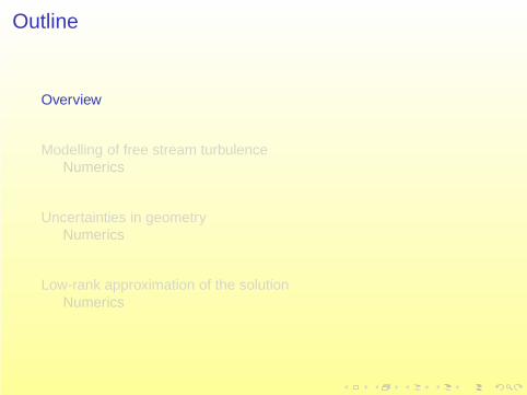
Outline

Overview

Modelling of free stream turbulenceNumerics

Uncertainties in geometryNumerics

Low-rank approximation of the solutionNumerics

Overview of uncertainties

Input:

1. Parameters (α, Ma, Re, ...)

2. Geometry

3. Parameters of turbulence

Uncertain output:

1. mean value and variance

2. exceedance probabilities P(u < u∗)

3. probability density and distribution functions.

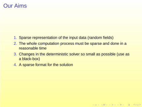
Our Aims

1. Sparse representation of the input data (random fields)

2. The whole computation process must be sparse and done in areasonable time

3. Changes in the deterministic solver so small as possible (use asa black-box)

4. A sparse format for the solution

Stochastical Methods overview

1. Monte Carlo Simulations (easy to implement, parallelisable,expensive, dim. indepen.).

2. Stoch. collocation methods with global or local polynomials (easyto implement, parallelisable, cheaper than MC, dim. depen.).

3. Stochastic Galerkin (difficult to implement, non-trivialparallelisation, the cheapest from all, dim. depen.)

Outline

Overview




Modelling of uncertainties in free stream turbulence

α

v

v

u

u’

α’v1

2

Random vectors v1 and v2 model turbulence in the atmosphere.

Truncated Polynomial Chaos Expansion

We represent CL in a Hermitian basis Hβ , β ∈ J .

CL(θ) =∑β∈J

Hβ(θ)CLβ , (1)

where θ a vector of random Gaussian variables, J is a multiindex setand β = (β1, ..., βj , ...) ∈ J a multiindex.

CLβ =1β!

∫Θ

Hβ(θ)CL(θ) P(dθ). (2)

CLβ ≈ 1β!

n∑i=1

Hβ(θi)CL(θi)wi , (3)

where weights wi and points θi are defined from sparseGauss-Hermite integration rule.

Uniform and Gaussian distributions of α and Ma

The following experiments are done for:Profiles: RAE-2822, Wilcox-k-w turbulence model

Turbulence intensity I = 0.001

mean st. deviation σ variance σ2

α 2.790 0.1 1.0e-2Ma 0.734 0.005 2.5e-5

Table: Mean values and standard deviations

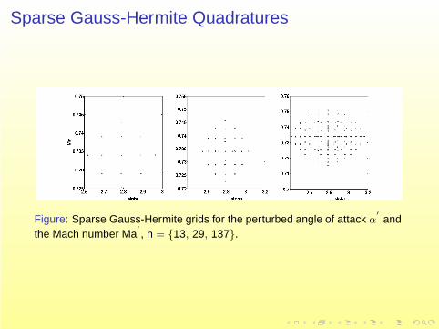
Sparse Gauss-Hermite Quadratures

Figure: Sparse Gauss-Hermite grids for the perturbed angle of attack α′

andthe Mach number Ma

′

, n = {13, 29, 137}.

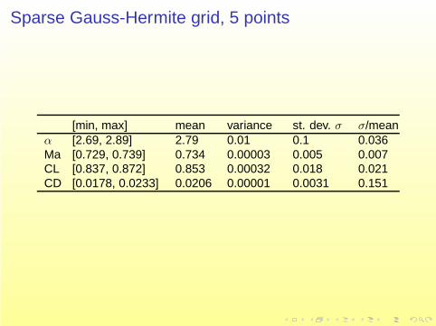
Sparse Gauss-Hermite grid, 5 points

[min, max] mean variance st. dev. σ σ/meanα [2.69, 2.89] 2.79 0.01 0.1 0.036Ma [0.729, 0.739] 0.734 0.00003 0.005 0.007CL [0.837, 0.872] 0.853 0.00032 0.018 0.021CD [0.0178, 0.0233] 0.0206 0.00001 0.0031 0.151

Sparse Gauss-Hermite grid, 13 points.


Sparse Gauss-Hermite grid, 29 points.


Table: Statistic obtained from 1500 MC simulations, α and Ma have Gaussiandistributions.


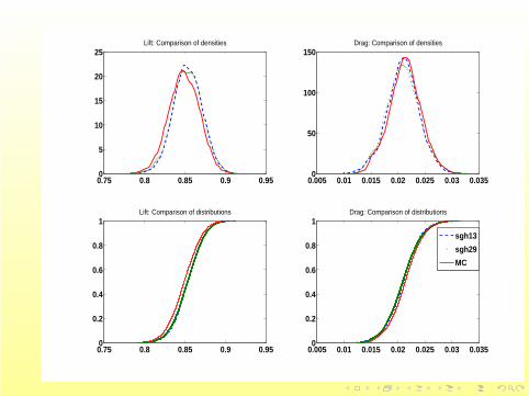
0.75 0.8 0.85 0.9 0.950

5

10

15

20

25Lift: Comparison of densities

0.005 0.01 0.015 0.02 0.025 0.03 0.0350

50

100

150Drag: Comparison of densities

0.75 0.8 0.85 0.9 0.950

0.2

0.4

0.6

0.8

1Lift: Comparison of distributions

0.005 0.01 0.015 0.02 0.025 0.03 0.0350

0.2

0.4

0.6

0.8

1Drag: Comparison of distributions

sgh13

sgh29

MC

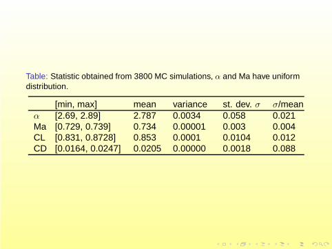
Table: Statistic obtained from 3800 MC simulations, α and Ma have uniformdistribution.


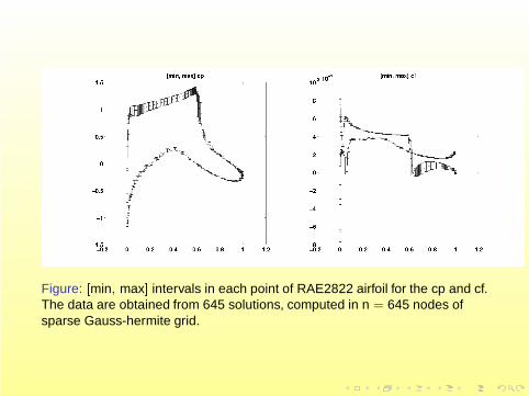
Figure: [min, max] intervals in each point of RAE2822 airfoil for the cp and cf.The data are obtained from 645 solutions, computed in n = 645 nodes ofsparse Gauss-hermite grid.

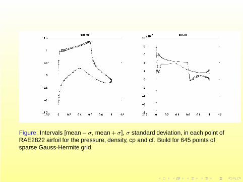
Figure: Intervals [mean− σ, mean + σ], σ standard deviation, in each point ofRAE2822 airfoil for the pressure, density, cp and cf. Build for 645 points ofsparse Gauss-Hermite grid.

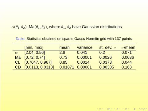
α(θ1, θ2), Ma(θ1, θ2), where θ1, θ2 have Gaussian distributions

Table: Statistics obtained on sparse Gauss-Hermite grid with 137 points.


Table: Comparison of results obtained by a sparse Gauss-Hermite grid (ngrid points) with 17000 MC simulations.

n 137 381 645 MC,17000

σCL

CL0.044 0.042 0.042 0.0145

σCD

CD0.163 0.159 0.16 0.1589

|CL−CL0|

CL7.6e-4 1.3e-3 1.6e-3 4.2e-4

|CD−CD0|

CD1.66e-2 1.46e-2 1.4e-2 2.1e-2

Outline

Overview




Uncertainties in geometry

Random boundary perturbations:∂Dε(ω) = {x + εκ(x , ω)n(x) : x ∈ ∂D}.where κ(x , ω) is a random field.

How to generate geometry with uncertainties ?Algorithm:

1. Assume cov. function cov(x , y) for random field κ(x , ω) given

2. Compute Cij := cov(xi , xj) for all grid points (in a sparse format!)

3. Solve eigenproblem Cφi = λiφi

4. Then κ(x , ω) ≈ ∑mi=1

√λiφiξi(ω), where ξi (ω) are uncorrelated

random variables.

Sparse approximation of dense matrix C is done in [Khoromskij,Litvinenko, Matthies, 2009]

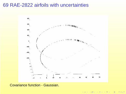
69 RAE-2822 airfoils with uncertainties

Covariance function - Gaussian.

Uncertainties in geometry

[min, max] mean variance, σ2

st. dev.σ

σ/mean

CL [0.828, 0.863] 0.8552 0.00002 0.0049 0.0058CD [0.017, 0.022] 0.0183 0.00000 0.00012 0.0065

PCE of order 1 with 3 random variables and sparse Gauss-Hermitegrid wite 25 points were used.

Outline

Overview




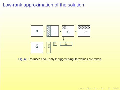
Low-rank approximation of the solution

U VΣ T=M

UVΣ∼

∼ ∼ T

=M∼

Figure: Reduced SVD, only k biggest singular values are taken.

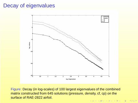
Decay of eigenvalues

0 0.5 1 1.5 2 2.5 3 3.5 4 4.5 5−20

−15

−10

−5

0

5

log, #eigenvalues

log

, va

lue

s

pressuredensitycpcf

Figure: Decay (in log-scales) of 100 largest eigenvalues of the combinedmatrix constructed from 645 solutions (pressure, density, cf, cp) on thesurface of RAE-2822 airfoil.

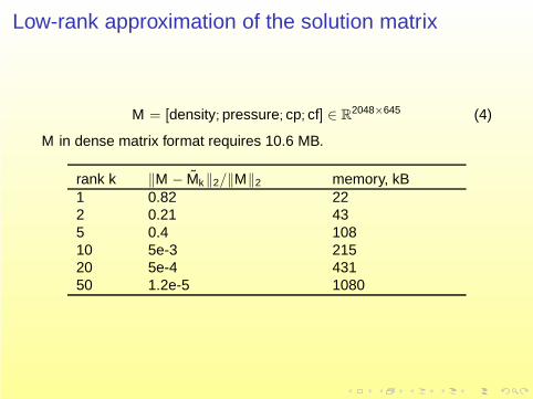
Low-rank approximation of the solution matrix

M = [density; pressure; cp; cf] ∈ R2048×645 (4)

M in dense matrix format requires 10.6 MB.

rank k ‖M − Mk‖2/‖M‖2 memory, kB1 0.82 222 0.21 435 0.4 10810 5e-3 21520 5e-4 43150 1.2e-5 1080

Literature

1. A.Litvinenko, H. G. Matthies, Sparse Data Representation ofRandom Fields, PAMM, 2009.

2. B.N. Khoromskij, A.Litvinenko, H. G. Matthies, Application ofhierarchical matrices for computing the Karhunen-Loeveexpansion, Springer, Computing, 84:49-67, 2009.

3. B.N. Khoromskij, A.Litvinenko, Data Sparse Computation of theKarhunen-Loeve Expansion, AIP Conference Proceedings,1048-1, pp. 311-314, 2008.

4. H. G. Matthies, Uncertainty Quantification with Stochastic FiniteElements, Encyclopedia of Computational Mechanics, Wiley,2007.

Acknowledgement

Elmar Zander

A Malab/Octave toolbox for stochastic Galerkin methods(KLE, PCE, sparse grids, tensors, many examples etc)

http://ezander.github.com/sglib/

Stochastic methods for uncertainty quantification in numerical aerodynamics

Engineering

Transcript of Stochastic methods for uncertainty quantification in numerical aerodynamics