Stochastic and Deterministic Search Algorithms for Global ...jskim/PhD08s_KimJS.pdfStochastic and...

s��<Æ~ÃÌ�� <Æ0A�7Hë�H

Stochastic and Deterministic Search

Algorithms for Global Optimization:

Molecular Annealing and Adaptive

Langevin Methods

¦�>�]� i¦�\��ª��· �Dø5� ��È��·Òeµ�\�l��§ ÚrÇa�Òeµ�\�ê�> ¿ÇÔaËc

N±Ó�§h�¤æ�æ·: &P�� #a��ÿb�ø� 'K�£� �ÐM� %�×m�'�× '�×ß��æ·

2008¿=> 2\Ôö

"��·7�Áþ�¬ 7�Áþ�xjS

�ä·h�§ >%K�Áþ�ÉÙ

ÊÏ�)K�ÐÏ�

Stochastic and Deterministic SearchAlgorithms for Global Optimization:Molecular Annealing and Adaptive

Langevin Methods¹ ?�

y�õ� �;M

l� ¹£�· ÎQ£ÈQm¹ãÃ�× £2Áþ�

2007� 11�

"��·×Qì ×QÅ

rÎØQ�

4�(

4�(�+ ÎQ£È Qm¹£�· �$Áþ�

2007� 12�

� y©�#îz�� ª

W � ~½Ó+þAðøÍ ª

�©�#î�ÃÌ ª

þj�� ñ ª

s�t�Äº ª

Stochastic and Deterministic Search

Algorithms for Global Optimization:

Molecular Annealing and Adaptive

Langevin Methods

by

Joon Shik Kim, B.S., M.S.

Dissertation

Presented to the Faculty of the Graduate School of

Seoul National University

in Partial Fulfillment

of the Requirements

for the Degree of

Doctor of Philosophy


February 2008

Abstract

Optimization is important in physical and engineering sciences for the

problems such as Lagrangian formalism in mechanics, finding the optimal elec-

tron density in quantum chemistry, designing minimum-cost networks in com-

puter science. Searching for global minima by overcoming local minima is a

fundamental issue in optimization.

This dissertation develops adaptive annealing methods which are physics-

based. Two optimization strategies drive a system from a high-entropic state

to a low-energetic state. The molecular annealing narrows the searching scope

down by controlling the acceptance ratio from higher to lower values. The adap-

tive Langevin equation uses the heavy ball’s inertia of mass and adaptive damp-

ing effect unlike in the ordinary Langevin equation in which the second-order

term in time is absent.

To obtain the predefined double stranded (ds) DNA in a large amount

from six fragments of single stranded (ss) DNAs, we performed molecular an-

nealing using silicon-based simulation and with wet-lab experiments. This com-

bination process solves the theorem-proving problem based on resolution refu-

tation.

Also, the heavy ball with friction (HBF) model with an adaptive damping

coefficient is proposed for the ball to search for a global minimum in Rosenbrock

and Griewank potentials. This adaptive damping coefficient was obtained from

iv

the geodesic of classical dynamics Lagrangian and its form is the negative time

derivative of the logarithmic function of the potential energy.

An associative memory retrieval experiment with partial pattern match-

ing with the DNA molecules is proposed for further study. Also, the charge

density on a conducting disk can be estimated with an adaptive Langevin equa-

tion. The data regarding this estimation is presented in this thesis. The two

algorithms developed in this dissertation are expected to be used in various

fields where global optimization is needed for the similar circumstances.

Keywords : DNA hybridization, simulated annealing, heavy ball with friction,

adaptive damping coefficient, global optimization

Student number : 98303-808

v

Contents

Abstract iv

List of Figures ix

Chapter 1 Introduction 1

Chapter 2 Background 5

2.1 Global Optimization . . . . . . . . . . . . . . . . . . . . . . . . 5

2.2 DNA Hybridization . . . . . . . . . . . . . . . . . . . . . . . . . 10

2.2.1 Theory . . . . . . . . . . . . . . . . . . . . . . . . . . . . 10

2.2.2 Application . . . . . . . . . . . . . . . . . . . . . . . . . 20

2.2.3 Further Study . . . . . . . . . . . . . . . . . . . . . . . . 25

2.3 Geodesic Optimization . . . . . . . . . . . . . . . . . . . . . . . 26

2.3.1 Theory . . . . . . . . . . . . . . . . . . . . . . . . . . . . 26

2.3.2 Application . . . . . . . . . . . . . . . . . . . . . . . . . 38

2.3.3 Further Study . . . . . . . . . . . . . . . . . . . . . . . . 39

2.4 Comparison of Two Algorithms . . . . . . . . . . . . . . . . . . 39

vi

Chapter 3 An Evolutionary Monte Carlo Algorithm for Predict-

ing DNA Hybridization 41

3.1 DNA Computing . . . . . . . . . . . . . . . . . . . . . . . . . . 41

3.1.1 DNA Computing in General . . . . . . . . . . . . . . . . 41

3.1.2 Adleman’s Hamiltonian Path Problem . . . . . . . . . . 42

3.1.3 Benenson et al.’s in vitro Cancer Drug Design . . . . . . 43

3.1.4 “Knight Problem” in 3×3 Chess Board . . . . . . . . . . 43

3.1.5 “Tic-Tac-Toe” by Deoxyribozyme Based Automation . . 43

3.2 Evolutionary Monte Carlo Method . . . . . . . . . . . . . . . . 44

3.3 In silico Algorithm for an Evolutionary Monte Carlo . . . . . . 48

3.3.1 Data Structure for DNA Hybridization . . . . . . . . . . 48

3.3.2 Attaching Process . . . . . . . . . . . . . . . . . . . . . . 50

3.3.3 Detaching Process . . . . . . . . . . . . . . . . . . . . . 50

3.4 Simulation Results for Theorem Proving . . . . . . . . . . . . . 51

3.5 Theorem Proving in vitro Experiment . . . . . . . . . . . . . . . 54

3.5.1 Design and Synthesis of Sequences . . . . . . . . . . . . 54

3.5.2 Quantitative Annealing of Oligonucleotides . . . . . . . . 55

3.5.3 Visualization of the Hybridized Mixture by Electrophoresis 55

3.5.4 Analysis of the Experiment Results . . . . . . . . . . . . 56

3.6 Conclusion . . . . . . . . . . . . . . . . . . . . . . . . . . . . . . 56

Chapter 4 A Global Minimization Algorithm Based on a Geodesic

of a Lagrangian Formulation of Newtonian Dynamics 61

vii

4.1 Derivation of an Adaptively Damped Oscillator . . . . . . . . . 61

4.2 Proof of Convergence to Global Minimum with Zero Point Con-

straint . . . . . . . . . . . . . . . . . . . . . . . . . . . . . . . . 64

4.3 Derivation of a Novel Adaptive Steepest Descent in a Discrete

Time Case . . . . . . . . . . . . . . . . . . . . . . . . . . . . . . 67

4.4 Examples of Global Optimization with Zero Point Constraint . . 69

4.5 Estimation of Charge Density on a Conducting Disk . . . . . . . 74

4.6 Conclusion . . . . . . . . . . . . . . . . . . . . . . . . . . . . . . 79

Chapter 5 Conclusion 81

Appendix A Trajectories of a Heavy Ball on Griewank Potential

from Initial Points (−10,−10) to (10,−10). 84

Bibliography 106

�ï �� 113

Acknowledgments 115

ÇÔ��+ ;³� 117

viii

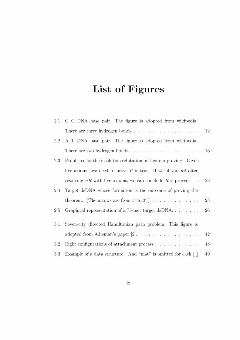
List of Figures

2.1 G–C DNA base pair. The figure is adopted from wikipedia.

There are three hydrogen bonds. . . . . . . . . . . . . . . . . . . 12

2.2 A–T DNA base pair. The figure is adopted from wikipedia.

There are two hydrogen bonds. . . . . . . . . . . . . . . . . . . 13

2.3 Proof tree for the resolution refutation in theorem-proving. Given

five axioms, we need to prove R is true. If we obtain nil after

resolving ¬R with five axioms, we can conclude R is proved. . 23

2.4 Target dsDNA whose formation is the outcome of proving the

theorem. (The arrows are from 5′ to 3′.) . . . . . . . . . . . . . 23

2.5 Graphical representation of a 75-mer target dsDNA. . . . . . . . 26

3.1 Seven-city directed Hamiltonian path problem. This figure is

adopted from Adleman’s paper [2]. . . . . . . . . . . . . . . . . 42

3.2 Eight configurations of attachment process. . . . . . . . . . . . . 48

3.3 Example of a data structure. And “mat” is omitted for each [][]. 49

ix

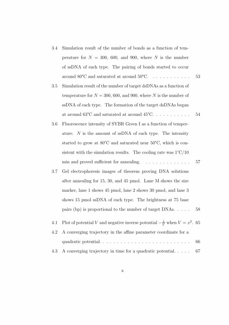
3.4 Simulation result of the number of bonds as a function of tem-

perature for N = 300, 600, and 900, where N is the number

of ssDNA of each type. The pairing of bonds started to occur

around 80°C and saturated at around 50°C. . . . . . . . . . . . 53

3.5 Simulation result of the number of target dsDNAs as a function of

temperature for N = 300, 600, and 900, where N is the number of

ssDNA of each type. The formation of the target dsDNAs began

at around 63°C and saturated at around 45°C. . . . . . . . . . . 54

3.6 Fluorescence intensity of SYBR Green I as a function of temper-

ature. N is the amount of ssDNA of each type. The intensity

started to grow at 80°C and saturated near 50°C, which is con-

sistent with the simulation results. The cooling rate was 1°C/10

min and proved sufficient for annealing. . . . . . . . . . . . . . 57

3.7 Gel electrophoresis images of theorem proving DNA solutions

after annealing for 15, 30, and 45 pmol. Lane M shows the size

marker, lane 1 shows 45 pmol, lane 2 shows 30 pmol, and lane 3

shows 15 pmol ssDNA of each type. The brightness at 75 base

pairs (bp) is proportional to the number of target DNAs. . . . . 58

4.1 Plot of potential V and negative inverse potential − 1V

when V = x2. 65

4.2 A converging trajectory in the affine parameter coordinate for a

quadratic potential. . . . . . . . . . . . . . . . . . . . . . . . . . 66

4.3 A converging trajectory in time for a quadratic potential. . . . . 67

x

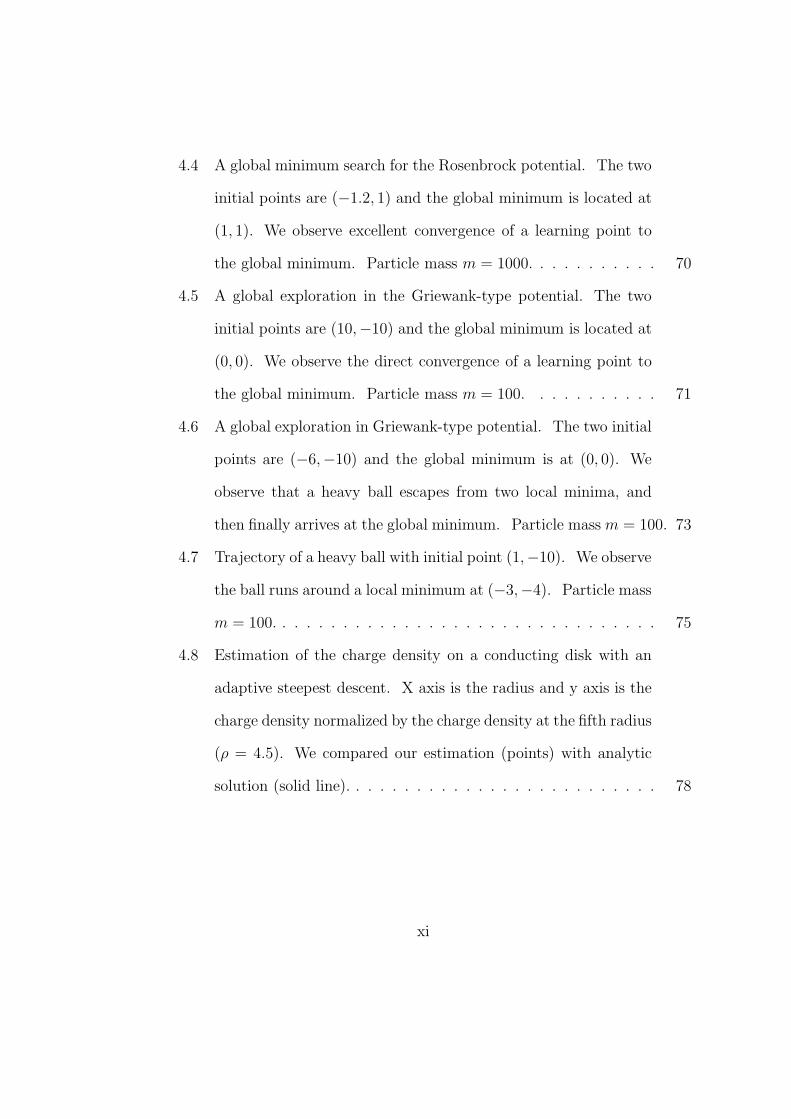
4.4 A global minimum search for the Rosenbrock potential. The two

initial points are (−1.2, 1) and the global minimum is located at

(1, 1). We observe excellent convergence of a learning point to

the global minimum. Particle mass m = 1000. . . . . . . . . . . 70

4.5 A global exploration in the Griewank-type potential. The two

initial points are (10,−10) and the global minimum is located at

(0, 0). We observe the direct convergence of a learning point to

the global minimum. Particle mass m = 100. . . . . . . . . . . 71

4.6 A global exploration in Griewank-type potential. The two initial

points are (−6,−10) and the global minimum is at (0, 0). We

observe that a heavy ball escapes from two local minima, and

then finally arrives at the global minimum. Particle mass m = 100. 73

4.7 Trajectory of a heavy ball with initial point (1,−10). We observe

the ball runs around a local minimum at (−3,−4). Particle mass

m = 100. . . . . . . . . . . . . . . . . . . . . . . . . . . . . . . . 75

4.8 Estimation of the charge density on a conducting disk with an

adaptive steepest descent. X axis is the radius and y axis is the

charge density normalized by the charge density at the fifth radius

(ρ = 4.5). We compared our estimation (points) with analytic

solution (solid line). . . . . . . . . . . . . . . . . . . . . . . . . . 78

xi

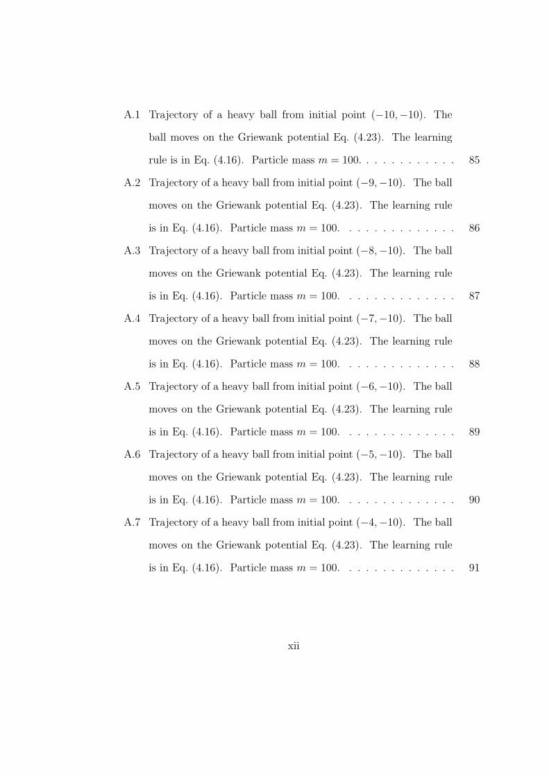
A.1 Trajectory of a heavy ball from initial point (−10,−10). The

ball moves on the Griewank potential Eq. (4.23). The learning

rule is in Eq. (4.16). Particle mass m = 100. . . . . . . . . . . . 85

A.2 Trajectory of a heavy ball from initial point (−9,−10). The ball

moves on the Griewank potential Eq. (4.23). The learning rule

is in Eq. (4.16). Particle mass m = 100. . . . . . . . . . . . . . 86
















xii










A.11 Trajectory of a heavy ball from initial point (0,−10). The ball





is in Eq. (4.16). Particle mass m = 100. The heavy ball does

not converge into a global minimum located at the origin. But if

we increase the mass of the ball, then the ball will converge into

the global minimum. . . . . . . . . . . . . . . . . . . . . . . . . 96




xiii






















xiv




xv

Chapter 1

Introduction

Two physical minimization strategies are presented in this dissertation. One

is for logical theorem proving by DNA computing and the other is for global

minimum search with the geodesic of Newtonian Lagrangian. These algorithms

correspond to information processes based on evolutionary and geodesic opti-

mization.

Regarding the tasks, we can perform logical theorem proving and global

minimum search with the stochastic and deterministic optimization. Stochastic

one is implemented with DNA by simulated annealing algorithm to get proof

target ds (double stranded) DNA. This algorithm is evolutionary for the use of

the variation and the selection processes. The deterministic algorithm adopts

the geodesic of a classical dynamics Lagrangian and it is used for searching

the global minimum. One constraint with potential function is that the value

is zero at global minimum. We can guarantee the convergence into the global

1

minimum by crashing behavior of a heavy ball into the singular inverse potential

in an affine parameter time. If this motion is viewed in an ordinary time, the

heavy ball will be seen to converge naturally with adaptive damping into the

global minimum.

Minimization of Gibbs free energy is the natural phenomena in chemistry.

This rule is related with the entropy maximization of environment and system.

Also Lagrangian formulation of Newtonian dynamics uses minimization of clas-

sical action. The calculus of variation is the method for implementing this min-

imization rule. We utilize these two optimization algorithms for implementing

information processes, such as, ”logical theorem proving” and ”global minimum

search.”

For the DNA computing, we use evolutionary algorithm to obtain the

target dsDNA. This evolutionary algorithm consists of population-based ran-

dom search and Metropolis selection. We just cool down the system slowly to

preserve the DNA tube in thermo-equilibrium. We use this strategy to drive the

DNA test tube into the global minimum state of Gibbs free energy. We compare

silicon-based simulation with wet-lab experiments and good agreement confirms

the validness of our evolutionary algorithm.

For the global minimization search, we use the minimization of time

integral for the square root of Newtonian Lagrangian. Affine parameter was

introduced in which the newly defined Lagrangian value is a constant value.

Invariance of this Lagrangian in affine parameter was used to derive a second–

order adaptively damped oscillator equation. This second–order equation was

2

discretized to obtain the first–order adaptive steepest descent learning rule. We

apply our adaptive steepest rule for Rosenbrock and Griewank potentials. And

the numerical results show a good performance for the ball to arrive at a global

minimum.

Now we presented two minimization algorithms for logical theorem prov-

ing and global minimization search. The first one is biochemical one and the

other is analytic rule. These strategies are novel in applying physical concepts

to artificial intelligence problems with minimization principles of biochemistry

and differential geometry. We hope our algorithms can be used for many ar-

eas, such as, neural networks, economics, and game theory where the global

minimum search finds the optimized parameters which reduce the cost.

Our novel contributions are as follows. We applied base-pair to base-

pair matching model to DNA hybridization within the Ising model framework.

Therefore Monte Carlo algorithm with only four parameters could simulate the

DNA hybridization. Three enthalpy values (G-C pair, A-T pair, others) and

one entropy value were sufficient for the simulation.

We extremized the time integral of the square root of classical mechanics

Lagrangian. Original classical dynamics arises from the extremization of the

time integral of classical mechanics Lagrangian. The difference between two

methods is whether taking the square root or not. We adopted the definition of

geodesic from the differential geometry and applied it to the classical mechanics

Lagrangian. And an adaptive damping coefficient for an adaptive Langevin

equation was obtained from the resulting geodesic equation.

3

In Chapter 2, we present the background for understanding the main

Chapters. In Chapter 3, we explain the molecular annealing algorithm for

DNA hybridization. In Chapter 4, we present an adaptive steepest descent, i.e.

adaptive Langevin equation. In Chapter 5, we draw conclusion. In Appendix,

geodesic trajectories on Griewank potential from twenty one initial conditions

are presented.

4

Chapter 2

Background

2.1 Global Optimization

A typical form of a global optimization is the minimization of a specific function

under a set of constraints. An example is to find the optimal use of each raw

material for a large amount of product with a bound of quantity on each raw

material. Scientific examples are as follows. In mechanics, Lagrangian formal-

ism is finding an extrema of the action. In quantum chemistry, if we find the

optimal local electron density which yields the minimum energy, we assert that

we solved the many-body problem. Protein folding problem consists in finding

the equilibrium configuration of the N atoms in a protein molecule with given

amino acid sequence, assuming the forces between the atoms are known. Also,

chemical equilibrium problems find the number and composition of the phases

of a mixture of chemical substances allowed to relax to equilibrium.

5

Engineering problems are as follows. Maximum clique problem asks for

the maximal number of mutually adjacent vertices in a given graph. Packing

problem is to place a number of k-dimensional objects of known shape within a

number of larger regions in such a way that there is no overlapping and a measure

of waste is minimized. Also, optimization for reducing cost and maximizing the

productivity has long been pursued by numerous inventions and ideas.

Approaches for these global optimization problems can be categorized

into three parts. The first one is the deterministic part. Branch and bound

methods and methods based on real algebraic geometry belong to the first part.

The second one is the stochastic and thermodynamics part. Simulated anneal-

ing and stochastic tunneling belong to the second part. The third one is the

heuristic and meta-heuristic part. Evolutionary algorithms and swarm-based

optimization algorithms belong to the third part.

We will study in the following paragraphs about the Kullback-Leibler di-

vergence and the negative log-likelihood. These two objects are two important

target functions to be minimized in artificial intelligence area. The Kullback-

Leibler divergence corresponds to the free energy and the negative log-likelihood

corresponds to the potential energy.

We need to understand the probabilistic formulation of a stochastic

process to understand the Kullback-Leibler divergence and the negative log-

likelihood. Throwing a dice and getting a number is a stochastic process, i.e.,

a process based on the probability. We can throw a dice for a hundred times or

a thousand times and trace the number on the dice at each time. Even though

6

such numerous and unpredictable sequences may refer to a random walk simu-

lation, the probabilistic model can be a more concise and simple representation

of the characteristics of a dice. Under this probabilistic model, each six number

has equal probability to be materialized and the probability of each number is

one sixth because the sum of each six equal probability has to be one.

The above simple probabilistic formulation is solid especially when the

number of related data is large. We can make a probabilistic model and just

find the appropriate parameters of this model. And it is known that many

distributions, such as the height and the weight follow the normal distribution

which is also called the Gaussian distribution. The Gaussian distribution is

centered at mean value and its spread is represented by standard deviation

(P = 1√2πσ

e−(x−<x>)2

2σ2 ). We made a hypothesis that an error cost will follow this

Gaussian distribution where an error cost is the square of the difference between

the answer of a teacher and that of a student. This probabilistic formulation

of an error cost enables us to use the techniques developed in thermodynamics

and statistical physics.

A system consisting of many reacting individuals is known to be within

Boltzmann distribution so long as it is in thermal equilibrium. The main reason

for this is that the Boltzmann distribution is the very condition in which the

number of possible states of both heat reservoir times that of small system con-

cerned is maximum. The entropy is defined as the Boltzmann constant times a

logarithmic function of the number of possible states. Therefore, the maximum

condition of the product value of the two numbers of each state equals to the

7

maximum condition of the sum of two entropies.

The above Boltzmann distribution is proportional to the exponential

function of the negative energy, i.e., the heat energy. We can consider that

an error cost is equivalent to the energy and can use the maximum entropy

condition for an error cost as in physical systems. This approach connects in-

formation science with physical science. For example, Shannon entropy is the

negative sum of each product of probability and its logarithmic function [25, 21].

And this Shannon entropy can be shown to be equal to the physical entropy.

In information science, Shannon entropy is the measure of an amount of infor-

mation and is a large value when the sequence of events is unpredictable. This

measure can be compared with the physical entropy which means the measure

of uncertainty.

Information analogy can also be found between Kullback-Leibler diver-

gence and Gibbs free energy. Gibbs free energy is defined as the enthalpy minus

the product of absolute temperature and the entropy. This Gibbs free energy

means the negative sum of two entropies of a system and an environment.

Therefore the maximum entropy principle minimizes the Gibbs free energy.

Likewise the Kullback-Leiber divergence should be minimized and the definition

of this divergence refers to the mean of the logarithmic function of a measurable

distribution minus the mean of the logarithmic function of a true distribution.

A measurable distribution is obtained by sampling and a true distribution is the

nature of the whole system. The mean value can be obtained with the measur-

able probability distribution. Minimization of the Kullback-Leibler divergence

8

corresponds to the estimation process for the true probability distribution of

the whole system based on the measurable sampling data [1, 12].

Also, we can regard an error cost as the energy and set the probability as

the exponential function of the negative energy. Then the minimization of the

negative logarithmic function of probability corresponds to the learning process.

This learning process decreases the error cost. Gradient descent, i.e. Langevin

equation, can be used for this optimization process. As the error cost becomes

smaller, the probability becomes larger.

The main purposes for machine learning and artificial intelligence are the

above two optimization processes. They are the minimization of the Kullback-

Leibler divergence and the minimization of the negative log-likelihood. There

are two approaches that can be taken in order to reach these two goals, i.e.,

a stochastic one which is probabilistic and a deterministic one which can be

formulated by a differential equation. The steepest descent corresponds to the

latter and Monte Carlo method belongs to the former. According to the steep-

est descent, the weight parameters are updated to the direction of the negative

gradient of an error cost, i.e., the steepest direction along the descent direction.

Regarding the variation made as an attempt under Monte Carlo method, we de-

termined whether to allow or deny this variation. Answers are given stochasti-

cally, i.e., with the random numbers. The example of this Monte Carlo method

is the Metropolis algorithm by which one can obtain the Boltzmann distribution.

9

2.2 DNA Hybridization

2.2.1 Theory

Ising model is a typical system where the Monte Carlo method is applicable.

This Ising model explains the ferromagnetic nature of iron, i.e., the reason

why iron can be made into be a magnet. This model makes a lattice where

the magnetic spin is located at each vertex. The whole spins can be arranged

to be parallel, by giving positive energy value to the two spins that are anti-

parallel and by giving negative value to two spins that are parallel. Therefore,

the ferromagnetic system can have a magnetic nature at an appropriate yet

low temperature. Of course, the energy distribution follows the Boltzmann dis-

tribution at each temperature. The Gaussian probability for the Boltzmann

distribution is the exponential function of the negative energy divided by the

product of the Boltzmann constant and the absolute temperature. We flipped

the randomly chosen spin and allowed the flipping according to the Metropolis

acceptance ratio of the energy change. And this operation made the whole spin

system into thermal equilibrium condition. This thermal equilibrium condition

is explained later in this section. Here the Metropolis acceptance ratio was

the exponential function of the negative energy change divided by the product

of the Boltzmann constant and the absolute temperature. In a formula form,

R = min{1, e−∆E/kBT}. R is the acceptance ratio, E is the energy, kB is the

Boltzmann constant, and T is the absolute temperature.

If we apply this Monte Carlo method to DNA molecules, an evolution-

10

ary Monte Carlo for predicting DNA hybridization can be devised [28]. DNA

is the information storage material for the biological process of an organism.

Basically, DNA consists of four kinds of base pairs namely, Adenine, Guanine,

Cytosine, and Thymine. A–T pair and G–C pair are Watson-Crick complemen-

tary pairs. At the same time, A–T pair is bound by two hydrogen bonds while

G–C pair is bound by three hydrogen bonds. RNA copies a portion of DNA by

complementary base pairs. And a copied messenger RNA (mRNA) is sent to a

Ribosome where the protein is generated according to mRNA sequence. This

is the central dogma of the genetic biology. Also the whole single stranded (ss)

DNA is converted into double stranded (ds) DNA by complementary copying

of each base pair. As a result of this operation, new cells are made to contain

the whole genetic information in equal numbers of DNA strands.

In regard to DNA molecules, we will describe the overall contents of DNA

hybridization using simulated annealing method. Molecular level intelligence is

required for the design of a clever drug aimed at a diagnosis or a cure in the gene

therapy. Therefore an appropriate DNA sequence design for detecting gene ma-

terial, for example microRNA, is required. In regards of these significances of

DNA level reaction, we propose an Ising model based simple DNA hybridiza-

tion rule for predicting the DNA hybridization. If temperature annealing is

considered, our algorithm is the implementation of the simulated annealing by

DNA molecules. We hope our algorithm will give a simple and clear under-

standing of mechanism in DNA hybridization. And we expect applications of

our simulation method to wet-lab experiment predictions.

11

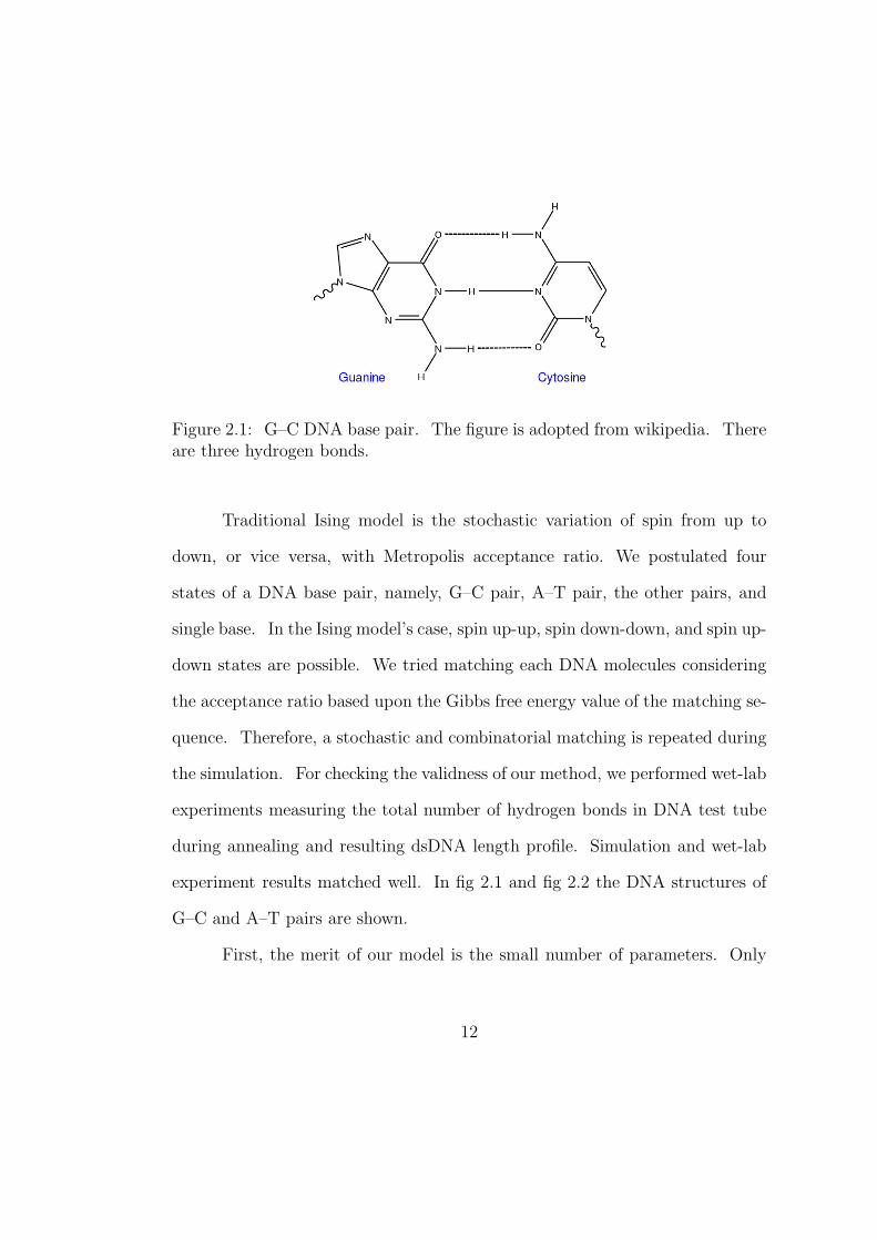
Figure 2.1: G–C DNA base pair. The figure is adopted from wikipedia. Thereare three hydrogen bonds.

Traditional Ising model is the stochastic variation of spin from up to

down, or vice versa, with Metropolis acceptance ratio. We postulated four

states of a DNA base pair, namely, G–C pair, A–T pair, the other pairs, and

single base. In the Ising model’s case, spin up-up, spin down-down, and spin up-

down states are possible. We tried matching each DNA molecules considering

the acceptance ratio based upon the Gibbs free energy value of the matching se-

quence. Therefore, a stochastic and combinatorial matching is repeated during

the simulation. For checking the validness of our method, we performed wet-lab

experiments measuring the total number of hydrogen bonds in DNA test tube

during annealing and resulting dsDNA length profile. Simulation and wet-lab

experiment results matched well. In fig 2.1 and fig 2.2 the DNA structures of

G–C and A–T pairs are shown.

First, the merit of our model is the small number of parameters. Only

12

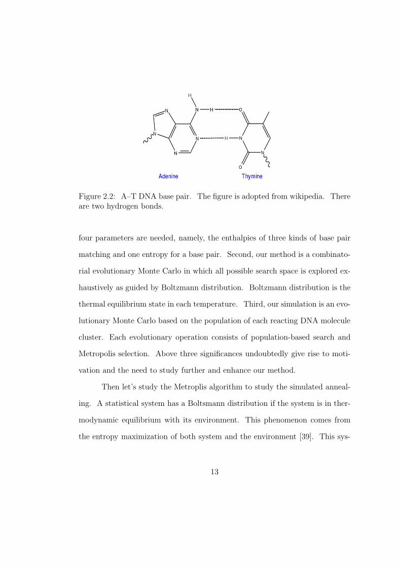
Figure 2.2: A–T DNA base pair. The figure is adopted from wikipedia. Thereare two hydrogen bonds.

four parameters are needed, namely, the enthalpies of three kinds of base pair

matching and one entropy for a base pair. Second, our method is a combinato-

rial evolutionary Monte Carlo in which all possible search space is explored ex-

haustively as guided by Boltzmann distribution. Boltzmann distribution is the

thermal equilibrium state in each temperature. Third, our simulation is an evo-

lutionary Monte Carlo based on the population of each reacting DNA molecule

cluster. Each evolutionary operation consists of population-based search and

Metropolis selection. Above three significances undoubtedly give rise to moti-

vation and the need to study further and enhance our method.

Then let’s study the Metroplis algorithm to study the simulated anneal-

ing. A statistical system has a Boltsmann distribution if the system is in ther-

modynamic equilibrium with its environment. This phenomenon comes from

the entropy maximization of both system and the environment [39]. This sys-

13

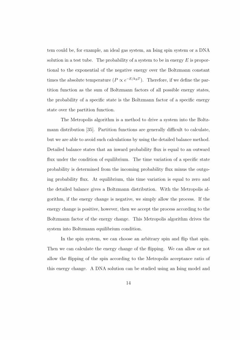
tem could be, for example, an ideal gas system, an Ising spin system or a DNA

solution in a test tube. The probability of a system to be in energy E is propor-

tional to the exponential of the negative energy over the Boltzmann constant

times the absolute temperature (P ∝ e−E/kBT ). Therefore, if we define the par-

tition function as the sum of Boltzmann factors of all possible energy states,

the probability of a specific state is the Boltzmann factor of a specific energy

state over the partition function.

The Metropolis algorithm is a method to drive a system into the Boltz-

mann distribution [35]. Partition functions are generally difficult to calculate,

but we are able to avoid such calculations by using the detailed balance method.

Detailed balance states that an inward probability flux is equal to an outward

flux under the condition of equilibrium. The time variation of a specific state

probability is determined from the incoming probability flux minus the outgo-

ing probability flux. At equilibrium, this time variation is equal to zero and

the detailed balance gives a Boltzmann distribution. With the Metropolis al-

gorithm, if the energy change is negative, we simply allow the process. If the

energy change is positive, however, then we accept the process according to the

Boltzmann factor of the energy change. This Metropolis algorithm drives the

system into Boltzmann equilibrium condition.

In the spin system, we can choose an arbitrary spin and flip that spin.

Then we can calculate the energy change of the flipping. We can allow or not

allow the flipping of the spin according to the Metropolis acceptance ratio of

this energy change. A DNA solution can be studied using an Ising model and

14

the Metropolis algorithm to produce the thermal equilibrium conditions of DNA

molecules in a test tube. This approach is described in Chapter 3 in detail.

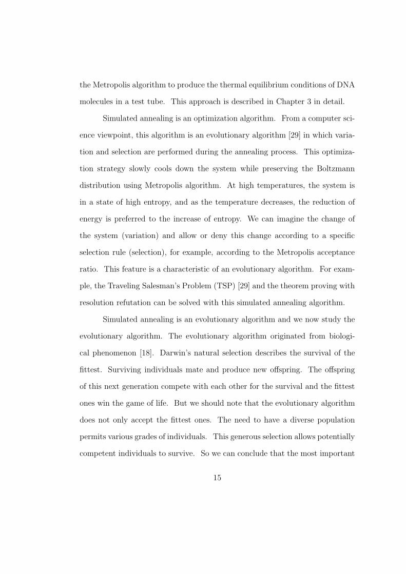
Simulated annealing is an optimization algorithm. From a computer sci-

ence viewpoint, this algorithm is an evolutionary algorithm [29] in which varia-

tion and selection are performed during the annealing process. This optimiza-

tion strategy slowly cools down the system while preserving the Boltzmann

distribution using Metropolis algorithm. At high temperatures, the system is

in a state of high entropy, and as the temperature decreases, the reduction of

energy is preferred to the increase of entropy. We can imagine the change of

the system (variation) and allow or deny this change according to a specific

selection rule (selection), for example, according to the Metropolis acceptance

ratio. This feature is a characteristic of an evolutionary algorithm. For exam-

ple, the Traveling Salesman’s Problem (TSP) [29] and the theorem proving with

resolution refutation can be solved with this simulated annealing algorithm.

Simulated annealing is an evolutionary algorithm and we now study the

evolutionary algorithm. The evolutionary algorithm originated from biologi-

cal phenomenon [18]. Darwin’s natural selection describes the survival of the

fittest. Surviving individuals mate and produce new offspring. The offspring

of this next generation compete with each other for the survival and the fittest

ones win the game of life. But we should note that the evolutionary algorithm

does not only accept the fittest ones. The need to have a diverse population

permits various grades of individuals. This generous selection allows potentially

competent individuals to survive. So we can conclude that the most important

15

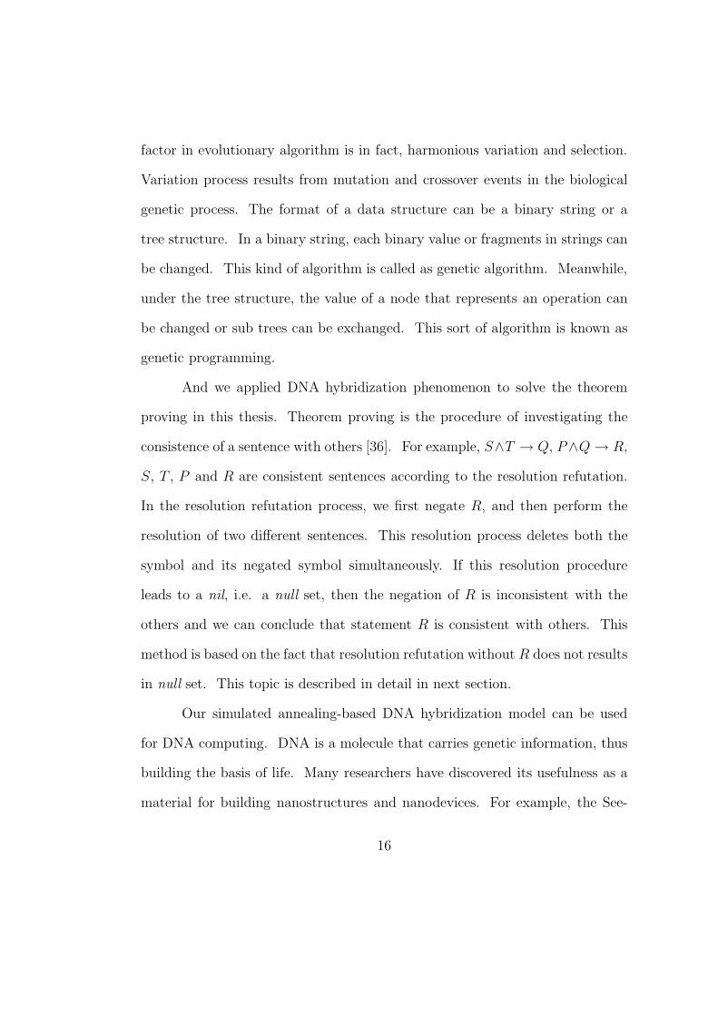
factor in evolutionary algorithm is in fact, harmonious variation and selection.

Variation process results from mutation and crossover events in the biological

genetic process. The format of a data structure can be a binary string or a

tree structure. In a binary string, each binary value or fragments in strings can

be changed. This kind of algorithm is called as genetic algorithm. Meanwhile,

under the tree structure, the value of a node that represents an operation can

be changed or sub trees can be exchanged. This sort of algorithm is known as

genetic programming.

And we applied DNA hybridization phenomenon to solve the theorem

proving in this thesis. Theorem proving is the procedure of investigating the

consistence of a sentence with others [36]. For example, S∧T → Q, P∧Q → R,

S, T , P and R are consistent sentences according to the resolution refutation.

In the resolution refutation process, we first negate R, and then perform the

resolution of two different sentences. This resolution process deletes both the

symbol and its negated symbol simultaneously. If this resolution procedure

leads to a nil, i.e. a null set, then the negation of R is inconsistent with the

others and we can conclude that statement R is consistent with others. This

method is based on the fact that resolution refutation without R does not results

in null set. This topic is described in detail in next section.

Our simulated annealing-based DNA hybridization model can be used

for DNA computing. DNA is a molecule that carries genetic information, thus

building the basis of life. Many researchers have discovered its usefulness as a

material for building nanostructures and nanodevices. For example, the See-

16

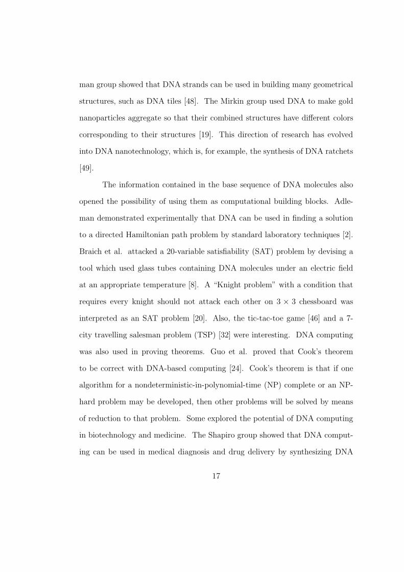
man group showed that DNA strands can be used in building many geometrical

structures, such as DNA tiles [48]. The Mirkin group used DNA to make gold

nanoparticles aggregate so that their combined structures have different colors

corresponding to their structures [19]. This direction of research has evolved

into DNA nanotechnology, which is, for example, the synthesis of DNA ratchets

[49].

The information contained in the base sequence of DNA molecules also

opened the possibility of using them as computational building blocks. Adle-

man demonstrated experimentally that DNA can be used in finding a solution

to a directed Hamiltonian path problem by standard laboratory techniques [2].

Braich et al. attacked a 20-variable satisfiability (SAT) problem by devising a

tool which used glass tubes containing DNA molecules under an electric field

at an appropriate temperature [8]. A “Knight problem” with a condition that

requires every knight should not attack each other on 3 × 3 chessboard was

interpreted as an SAT problem [20]. Also, the tic-tac-toe game [46] and a 7-

city travelling salesman problem (TSP) [32] were interesting. DNA computing

was also used in proving theorems. Guo et al. proved that Cook’s theorem

to be correct with DNA-based computing [24]. Cook’s theorem is that if one

algorithm for a nondeterministic-in-polynomial-time (NP) complete or an NP-

hard problem may be developed, then other problems will be solved by means

of reduction to that problem. Some explored the potential of DNA computing

in biotechnology and medicine. The Shapiro group showed that DNA comput-

ing can be used in medical diagnosis and drug delivery by synthesizing DNA

17

computing drugs in vitro with restriction enzymes [6].

In the core of all the DNA experiments above lies the sequence-specific

DNA hybridization process. Thus, modeling the DNA hybridization process

has been so important that numerous design tools for DNA hybridization have

been suggested by many researchers. For example, the SantaLucia group ex-

tensively studied DNA melting phenomena at the nucleotide level providing

thermodynamic parameters for the nearest-neighbor (NN) model [26, 7]. The

Garzon group’s electronic analogs of DNA (EDNA) system is another tool for

DNA hybridization, which is also based on the NN model [22]. EDNA sys-

tem provides a way of performing biomolecular computing with silicon-based

computers. Shin et al. developed a multiobjective evolutionary optimization

technique to design optimal sequences [44]. They obtained these sequences by

the optimization of the six fitness measures, which are similarity, H-measure,

secondary structure, continuity, melting temperature, and GC content. Most

of these studies aimed at helping DNA code design and focused on the base

sequences within NN-model framework.

In this thesis, we propose a novel Monte Carlo algorithm for simulating

DNA hybridization and use evolutionary computation to take into account the

combinatorial effect of DNA molecules and simplified thermodynamics of DNA

hybridization. In our previous study, we proposed an evolutionary algorithm

that uses a Markov chain Monte Carlo approach to identify unknown config-

urations with probabilistic modeling of search space [51]. In this work, rather

than identifying each possible configuration of DNA strands with probabilistic

18

modeling, we combine a population-based evolutionary search and a Metropolis

selection. Random selection of two parent strands will be in proportion to the

number of those within the population so that we are actually performing a

population-based search. After one of every possible option of DNA hybridiza-

tion or denaturation is chosen, the Metropolis selection allows or denies that

particular process, and eventually drives the system into a minimum-free-energy

configuration of the system at the given temperature. After reaching equilib-

rium, simulated annealing is used to keep the system in thermal equilibrium as

it is cooled [29]. The evolutionary nature of the Metropolis algorithm and sim-

ulated annealing has been studied as a possible evolutionary mutation operator

[16]. In our simulation, we have four parameters that can be extracted from

other experiments [30]. In this sense, our algorithm is minimal and powerful in

simulating reacting DNA molecules, whereas the NN model uses more than 20

parameters [26, 7, 22]. This reduced number of parameters will be effective in

simulating very long DNA strands.

Our evolutionary Monte Carlo method is applied to theorem-proving by

resolution refutation in artificial intelligence [36, 31]. This theorem-proving is

a logical inference process from given statements and logical relations among

them. In the simulation, we measure the number of bonds and the number of

target dsDNA strands as a function of temperature. The increasing number

of target dsDNA in the simulation corresponds to the completion of theorem-

proving. To confirm our algorithm, we perform wet-lab experiments with syn-

thetic DNAs, in which we obtain the number of bonds by measuring SYBR

19

Green I fluorescence. We also measure the concentration of the target dsDNA

by gel electrophoresis when test samples arrive at a temperature well below the

melting temperature, which confirms the formation of the target dsDNA. The

numerical simulation result of the number of bonds matches the experimental

data very well.

2.2.2 Application

DNA computing is an effort to solve computational problems with standard

biochemical techniques. For example, Adleman solved the seven city directed

Hamiltonian path problem [2]. This problem was solved when we found the

path in which a traveler visits every city once along the directed graphical

path. Adleman encoded the city and the edge by 20-mer DNA sequence and

found the molecular dsDNA path satisfying the condition to the solution. The

total length of the city and edge compound can be found by the electrophoresis

and whether the DNA molecule contains a particular city was examined by a

biotin bead separation method. Biotin can be bound to ssDNA of a particular

sequence. And if this ssDNA is attached to other ssDNA, then biotin compound

can be attracted magnetically. Therefore one can separate the molecules that

contain the particular pattern of DNA sequence.

Similar approach can be applied to “Tic-Tac-Toe” [46] and “Knight prob-

lem” [20] in which solution was transformed into SAT problem and the exact

solution was found by deleting various candidates one by one. SAT is the prob-

lem in which “True” or “False” value is assigned to the logic statements. These

20

logic statements are connected by “OR” then the groups of statements are con-

nected by “AND”. They searched for the combination of the truth values of

these statements that made the whole sentence “True”. In addition, an effort

to make a diagnosis and to release the drug for lung cancer was carried on by

Benenson et al. based on the genetic information and DNA computing [6]. A

lung cancer patient has high concentrations of certain restriction enzymes so

that these enzymes disconnect the diagnosis part of the DNA drug. And if

this diagnosis part is dispatched appropriately, then the genetic cancer drug

is released to depress the gene expression of cancer cell. This experiment was

performed in vitro in test tube.

This thesis presents a study of a molecular theorem proving based on

resolution refutation. S ∧ T → Q, P ∧ Q → R and the question is whether

R is consistent with other statements as long as S, T , and P is true. In the

following sentences, → means “Implication”, ¬ means “Negation”, ∨ means

“OR”, and ∧ means “AND”. For example, a fever (S) and a cough (T) imply

a cold (Q), while a cold (Q) and a headache (P) imply the need to go to the

hospital (R). Based on this assumption, the question is whether it is necessary

to go to hospital or not, if one has a fever (S), a cough (T), and a headache (P).

Table 2.1 shows the statements encoded by DNA sequences.

To solve this problem, one should note that (p → q) being equal to

(¬p∨ q). If p is true and q is true, then the truth sets of both p and q becomes

universal set. Therefore the truth set of p belongs to the truth set of q which

means the statement is true. (¬p∨ q) is also true because q is true. If p is true

21

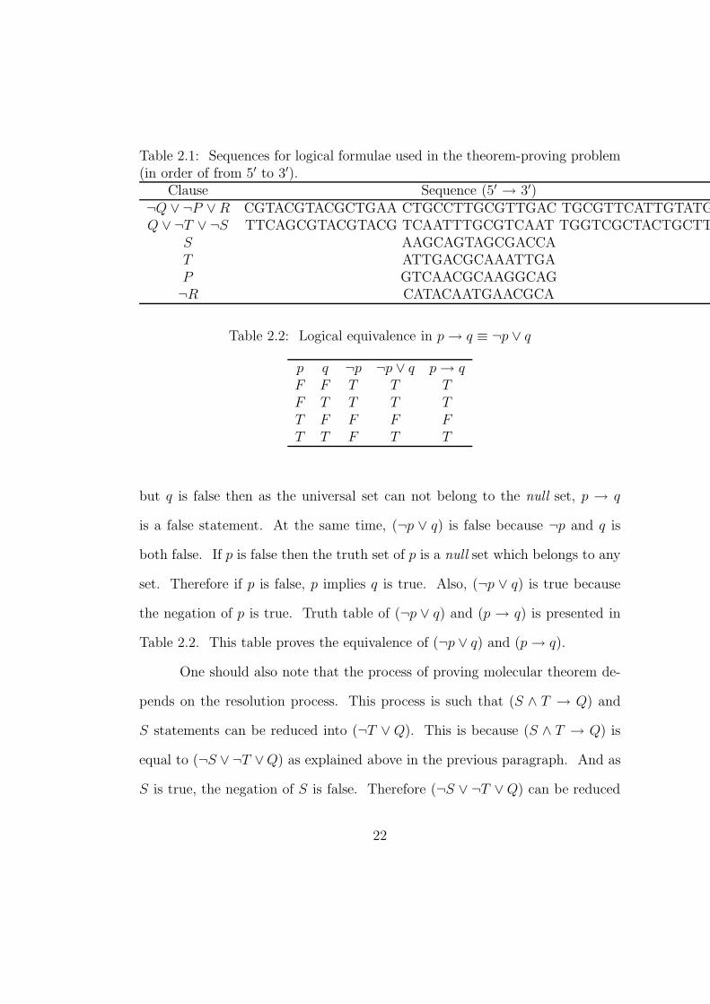
Table 2.1: Sequences for logical formulae used in the theorem-proving problem(in order of from 5′ to 3′).

Clause Sequence (5′ → 3′)¬Q ∨ ¬P ∨ R CGTACGTACGCTGAA CTGCCTTGCGTTGAC TGCGTTCATTGTATGQ ∨ ¬T ∨ ¬S TTCAGCGTACGTACG TCAATTTGCGTCAAT TGGTCGCTACTGCTT

S AAGCAGTAGCGACCAT ATTGACGCAAATTGAP GTCAACGCAAGGCAG¬R CATACAATGAACGCA

Table 2.2: Logical equivalence in p → q ≡ ¬p ∨ q

p q ¬p ¬p ∨ q p → qF F T T TF T T T TT F F F FT T F T T

but q is false then as the universal set can not belong to the null set, p → q

is a false statement. At the same time, (¬p ∨ q) is false because ¬p and q is

both false. If p is false then the truth set of p is a null set which belongs to any

set. Therefore if p is false, p implies q is true. Also, (¬p ∨ q) is true because

the negation of p is true. Truth table of (¬p ∨ q) and (p → q) is presented in

Table 2.2. This table proves the equivalence of (¬p ∨ q) and (p → q).

One should also note that the process of proving molecular theorem de-

pends on the resolution process. This process is such that (S ∧ T → Q) and

S statements can be reduced into (¬T ∨ Q). This is because (S ∧ T → Q) is

equal to (¬S ∨¬T ∨Q) as explained above in the previous paragraph. And as

S is true, the negation of S is false. Therefore (¬S ∨ ¬T ∨ Q) can be reduced

22

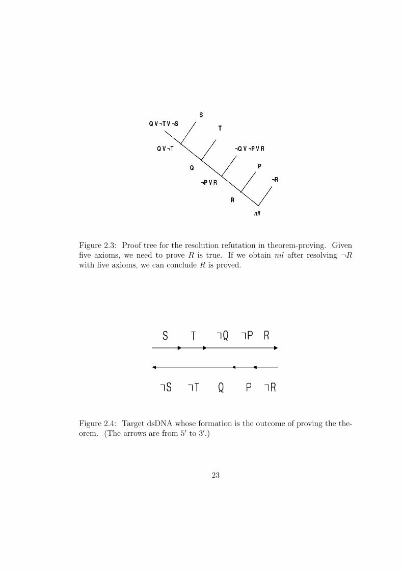
Figure 2.3: Proof tree for the resolution refutation in theorem-proving. Givenfive axioms, we need to prove R is true. If we obtain nil after resolving ¬Rwith five axioms, we can conclude R is proved.

Figure 2.4: Target dsDNA whose formation is the outcome of proving the the-orem. (The arrows are from 5′ to 3′.)

23

to (¬T ∨ Q). Likewise, S ∧ T → Q, P ∧ Q → R, S, T , P are resolved into R.

This process is shown in fig 2.3. At this moment, the same question from the

above paragraph should be asked again, the question being whether or not R is

consistent with other statements. If we negate R as ¬R and make a resolution

with other statements, we can obtain null set as a result of R and ¬R being

resolved into nil. Meanwhile a nil means being contradictory. Therefore we are

able to conclude that the negation of R is a false operation and R is consistent

with other statements. Therefore, if one has a fever, a cough, and a headache

then he has to go to the hospital. Resolution process is shown in fig. 2.3 and

75-mer target dsDNA representing nil is shown in fig. 2.4.

We encoded S by 15 base pairs of ssDNA and encoded ¬S by Watson-

Crick complementary pairs of S. That is to say A is replaced by T and G is

replaced by C. Therefore two 45-mer ssDNAs would mean (S ∧ T → Q) and

(P ∧Q → R). At the same time, four 15-mer ssDNAs mean S, T , P , and ¬R.

The resolution process corresponds to the binding of S with ¬S under Watson-

Crick base pair matching. Therefore 75-mer target dsDNA means the nil in the

theorem proving problem. This 75-mer target dsDNA is the one in which all six

fragments are bound simultaneously. In the experiment, we slowly cooled the

test tube that contained six kinds of ssDNA fragments. Then we measured the

SYBR Green I fluorescence during the annealing. SYBR Green I is attached to

the hydrogen bonds of dsDNA and emits fluorescence when laser light is shed

upon it. We compared this fluorescence curve with our simulator’s result and

obtained a good agreement.

24

After the cooling of the test tube, the solution undergoes an electrophore-

sis experiment. Electrophoresis experiment consists of a voltage gradient and

a gel with fluorescence ingredients. If DNA is attracted electrically, the viscous

force is proportional to the length of DNA molecules. Therefore sorting in ac-

cordance with the DNA length becomes possible. Also, during the drag, the

DNA molecule collects the fluorescence ingredients. Therefore, when we place

the cooled solution containing 75-mer dsDNA under the electrophoresis experi-

ment, we can observe a highlighting 75-mer band. This 75-mer length is known

by comparing the band with the known DNA marker ladder of known length.

This outcome results in an agreement with our in silico simulation result, where

most of the fragments participate in the formation of 75-mer target dsDNA.

2.2.3 Further Study

The spin glass system is the Ising like system, but coupling constants follow

Gaussian distribution. Hopfield and Amit found that this spin glass model can

be used as an associative memory recall model in which the coupling constant is

the sum of the tensor product of each memory vector [4]. Deaton and Garzon

reported that DNA system is similar to the spin glass system [13]. Therefore an

associative memory recall by DNA molecules can be studied in the framework

of Hopfield model.

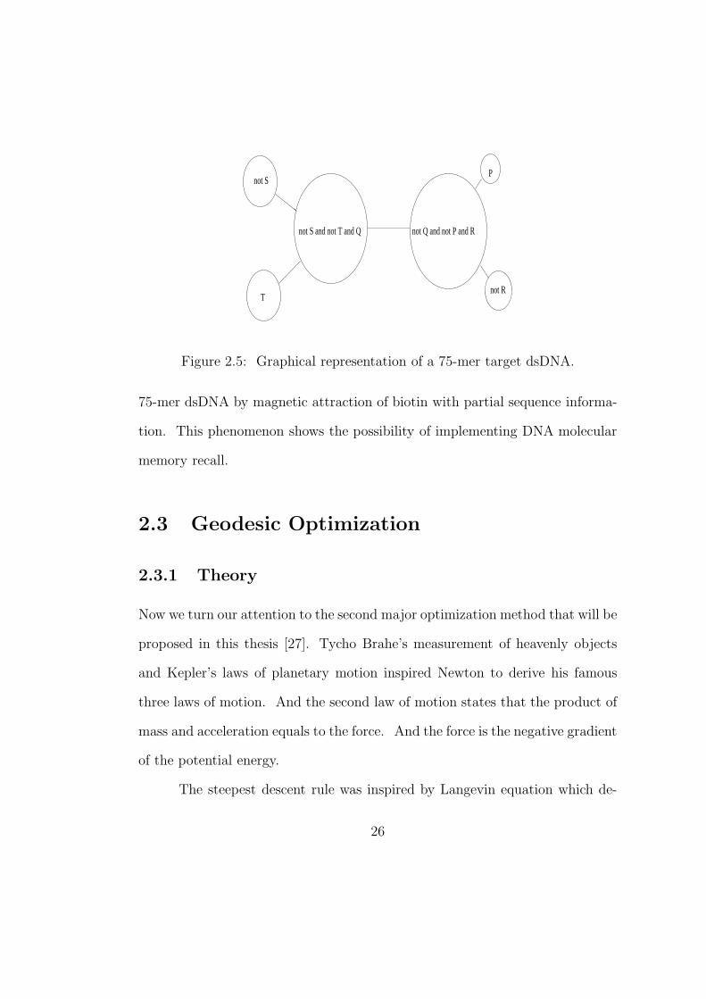
In our experiment 75-mer target dsDNA represents the graph pattern

as shown in Fig 2.5. And each node can be reached by the graphical path. If

one uses biotin and ssDNA compound, they will be able to retrieve the whole

25

not S

not S and not T and Q not Q and not P and R

P

not R T

Figure 2.5: Graphical representation of a 75-mer target dsDNA.

75-mer dsDNA by magnetic attraction of biotin with partial sequence informa-

tion. This phenomenon shows the possibility of implementing DNA molecular

memory recall.

2.3 Geodesic Optimization

2.3.1 Theory

Now we turn our attention to the second major optimization method that will be

proposed in this thesis [27]. Tycho Brahe’s measurement of heavenly objects

and Kepler’s laws of planetary motion inspired Newton to derive his famous

three laws of motion. And the second law of motion states that the product of

mass and acceleration equals to the force. And the force is the negative gradient

of the potential energy.

The steepest descent rule was inspired by Langevin equation which de-

26

scribes the Newton’s second law with a damping term of being proportional to

the negative velocity. Unlike Newton’s second law where the time derivative is

the second-order, Langevin equation is the first-order in time derivative and the

two equations have the gradient term in common.

The fatal limit of the steepest descent is that it can not overcome the

local minimum. Therefore, it can not ensure the convergence of a system into

a global minimum state. The heavy ball with friction (HBF) model uses the

second-order acceleration and a damping term in order to use the inertia of mass

so to overcome this limit. But the damping coefficient of HBF is constant that

dynamic path of a ball varies from being overdamped to being underdamped as

the damping coefficient decreases.

We searched for an appropriate adaptive damping coefficient for this HBF

model and got a hint from the geometric method in natural gradient [3]. The

natural gradient uses Fisher information which is the metric of Kullback-Leibler

divergence. By adopting this Fisher information, the plateau phenomenon of

the back-propagation neural networks method has been defeated. The back-

propagation is the neural networks learning method where data proceed from

input layer to hidden layer, then proceed to the output node [40]. After this

forward update of node value according to the weights, the difference between

a teacher’s true value and a student’s answer is propagated backwards by ad-

justing the weights by chain rule. And this back-propagation undergoes a long

time of plateau period before entering into an optimized state.

Our approach was to apply a geometric method to Newtonian mechanics

27

where metric comes from the Lagrangian formulation of classical mechanics.

Newton’s mechanics can be formulated by the Lagrangian formulation in which

the Lagrangian is defined as kinetic energy minus potential energy. The time

integral of this Lagrangian along the correct path is extremal, and this correct

path is the exact path of classical particle. The equation of motion of this

calculus of variation method can be obtained from the fact that a small variation

of the correct path does not much change the time integral of Lagrangian.

Resulting equation is the Euler–Lagrange equation and Newton’s second law

can be easily be derived from this Euler–Lagrange equation with the classical

Lagrangian.

Riemannian approach was studied for Newton’s second law [10]. The

metric can be obtained from the Lagrangian of classical mechanics. The met-

ric is the coefficient of each variable’s contribution to the curve length in the

manifold. For example, the sphere and the cylinder are in three dimensional

space and the curve length on each object’s surface is described differently. And

the coefficient of each curve is the intrinsic nature of each manifold [15]. We

choose one time and n dimensional space coordinate and calculated the geodesic

equation from the classical mechanics metric. And this metric was originated

from classical mechanics Lagrangian. Next, Euler–Lagrange equation was used

to realize an equation of motion. Geodesic curve, which is the shortest path

connecting two points on the manifold, was obtained as a result of this process.

In doing this calculation, we had two kinds of time, the one being the affine time

in which the speed of curve is unity on the (1 + n)D manifold and the other

28

being ordinary time. The affine parameter time corresponds to the proper time

in Minkowski space as we will see later in this section.

The geodesic equation in affine time is Newton’s second law with nega-

tive inverted potential. Therefore the singularity arises at the position where

the potential value is zero. The geodesic equation in ordinary time is an adap-

tively damped oscillator equation where the damping coefficient is negative time

derivative of the logarithmic function of the potential. The convergence of the

heavy ball is confirmed by the singularity in an affine time, and this singular

behavior is seen to be a damped convergence into a global minimum from the or-

dinary time viewpoint. This phenomenon is similar to that of blackhole where

Schwarzschild’s radius is singular [14]. And because of the slow time elapse due

to this singularity, the falling object is seen to be damped at that radius. The

man riding on an object simply passes the radius and collapses into the center

of the blackhole.

In short, we can make an analogy between blackhole’s singular nature

and the convergence of an adaptive steepest learning rule. And this damping

coefficient is the negative time derivative of the logarithmic function of an error

cost.

Next, we summarize the contents of geodesic optimization. Finding the

global minimum with escaping local minima is an important topic in physics,

machine learning, and even in economics. This is important because this global

minimization finds the most stable and lowest error cost state. Previously, there

have been efforts to devise a global minimum search algorithm based on a me-

29

chanical model. The heavy ball with friction model is an example. Although

such an approach tried to find a global minimum in some potentials, such as

Rosenbrock and Griewank, the need for determining an appropriate damping

coefficient still remains. In this thesis, we present that the appropriate damp-

ing coefficient for a heavy ball with friction (HBF) model is the negative time

derivative of the logarithmic function of the error cost. This coefficient was

derived from Euler–Lagrange equation of classical mechanics metric. Our ap-

proach shows that the geodesic of Newtonian dynamics Lagrangian is a good

candidate for global minimization algorithm.

We considered the time as an equivalent variable as space coordinates.

And we defined an affine parameter as an independent parameter replacing the

time. A new Lagrangian was also defined from classical mechanics Lagrangian

and this new Lagrangian is a constant in the evolution of affine parameter.

By solving Euler–Lagrange equation for this newly defined Lagrangian, we can

obtain an adaptively damped equation whose damping coefficient is the negative

time derivative of the logarithmic function of the error cost. We discretized this

second–order damped equation into the first order adaptive steepest descent

learning rule. An adaptive momentum parameter and an adaptive learning rate

were derived during the discretization. We confirmed the validness of our global

minimization algorithm in Rosenbrock potential and Griewank potentials. The

only constraint of an error cost potential is that this error cost should have a zero

value at the global minimum weight coordinate. This constraint guarantees the

convergence of a heavy ball into the global minimum site.

30

The derivation of an appropriate damping coefficient for HBF model

from the geodesic of classical Lagrangian metric is a novel contribution. We

also treated the time coordinate as an equivalent variable as the weight space

variables. This approach is similar to that of the general theory of relativity.

Our algorithm’s convergence is guaranteed from the equivalence between the

trajectories of Euler–Lagrange equation in both affine parameter and ordinary

time coordinate [14]. In an affine parameter space, the constraint of an ordinary

time potential, that is, the error cost having a zero value at the global minimum,

produces a singularity in an affine parameter potential. And the mathematical

form of this singularity is the negative inverse of the potential.

We are trying to solve the global optimization problem by an adaptive

Langevin equation. And the derivation of Langevin equation is as follows. In

Brownian motion, the particle feels the viscous force and random noise. We

can describe this motion as a second–order differential equation. If the mass is

set to zero, then the equation is reduced to a first–order differential equation.

Under statistical learning theory, this equation corresponds to a steepest descent

rule.

In formular description,

md2x

dt2= −µ

dx

dt+ δ + F, (2.1)

(2.2)

δ is a noise term and F represents an external force. And if m = 0 then above

31

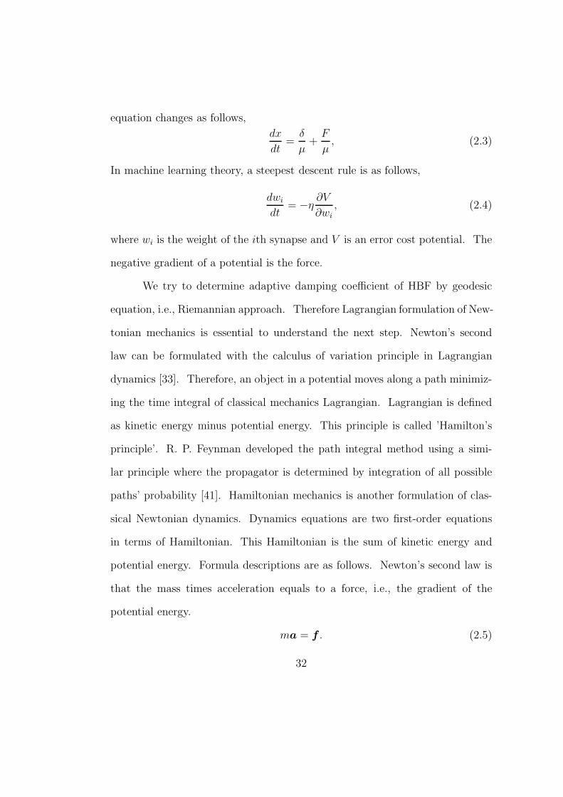
equation changes as follows,

dx

dt=

δ

µ+

F

µ, (2.3)

In machine learning theory, a steepest descent rule is as follows,

dwi

dt= −η

∂V

∂wi, (2.4)

where wi is the weight of the ith synapse and V is an error cost potential. The

negative gradient of a potential is the force.

We try to determine adaptive damping coefficient of HBF by geodesic

equation, i.e., Riemannian approach. Therefore Lagrangian formulation of New-

tonian mechanics is essential to understand the next step. Newton’s second

law can be formulated with the calculus of variation principle in Lagrangian

dynamics [33]. Therefore, an object in a potential moves along a path minimiz-

ing the time integral of classical mechanics Lagrangian. Lagrangian is defined

as kinetic energy minus potential energy. This principle is called ’Hamilton’s

principle’. R. P. Feynman developed the path integral method using a simi-

lar principle where the propagator is determined by integration of all possible

paths’ probability [41]. Hamiltonian mechanics is another formulation of clas-

sical Newtonian dynamics. Dynamics equations are two first-order equations

in terms of Hamiltonian. This Hamiltonian is the sum of kinetic energy and

potential energy. Formula descriptions are as follows. Newton’s second law is

that the mass times acceleration equals to a force, i.e., the gradient of the

potential energy.

ma = f . (2.5)

32

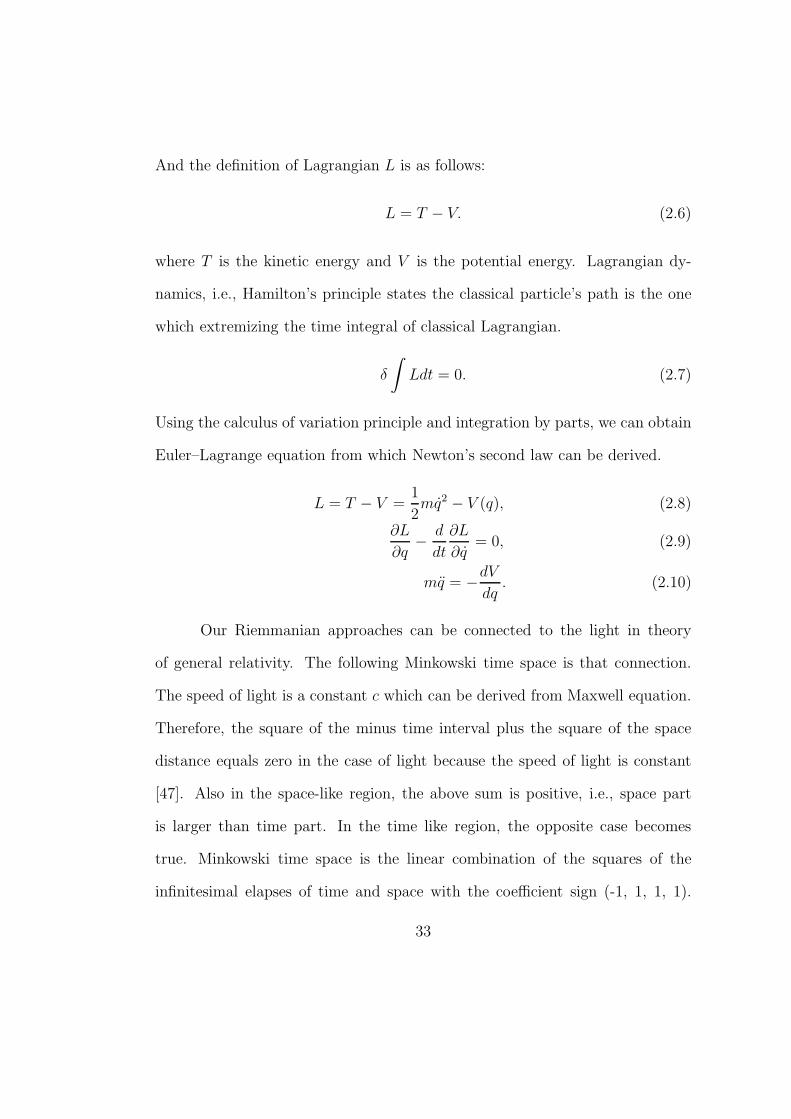
And the definition of Lagrangian L is as follows:

L = T − V. (2.6)

where T is the kinetic energy and V is the potential energy. Lagrangian dy-

namics, i.e., Hamilton’s principle states the classical particle’s path is the one

which extremizing the time integral of classical Lagrangian.

δ

∫

Ldt = 0. (2.7)

Using the calculus of variation principle and integration by parts, we can obtain

Euler–Lagrange equation from which Newton’s second law can be derived.

L = T − V =1

2mq2 − V (q), (2.8)

∂L

∂q− d

dt

∂L

∂q= 0, (2.9)

mq = −dV

dq. (2.10)

Our Riemmanian approaches can be connected to the light in theory

of general relativity. The following Minkowski time space is that connection.

The speed of light is a constant c which can be derived from Maxwell equation.

Therefore, the square of the minus time interval plus the square of the space

distance equals zero in the case of light because the speed of light is constant

[47]. Also in the space-like region, the above sum is positive, i.e., space part

is larger than time part. In the time like region, the opposite case becomes

true. Minkowski time space is the linear combination of the squares of the

infinitesimal elapses of time and space with the coefficient sign (-1, 1, 1, 1).

33

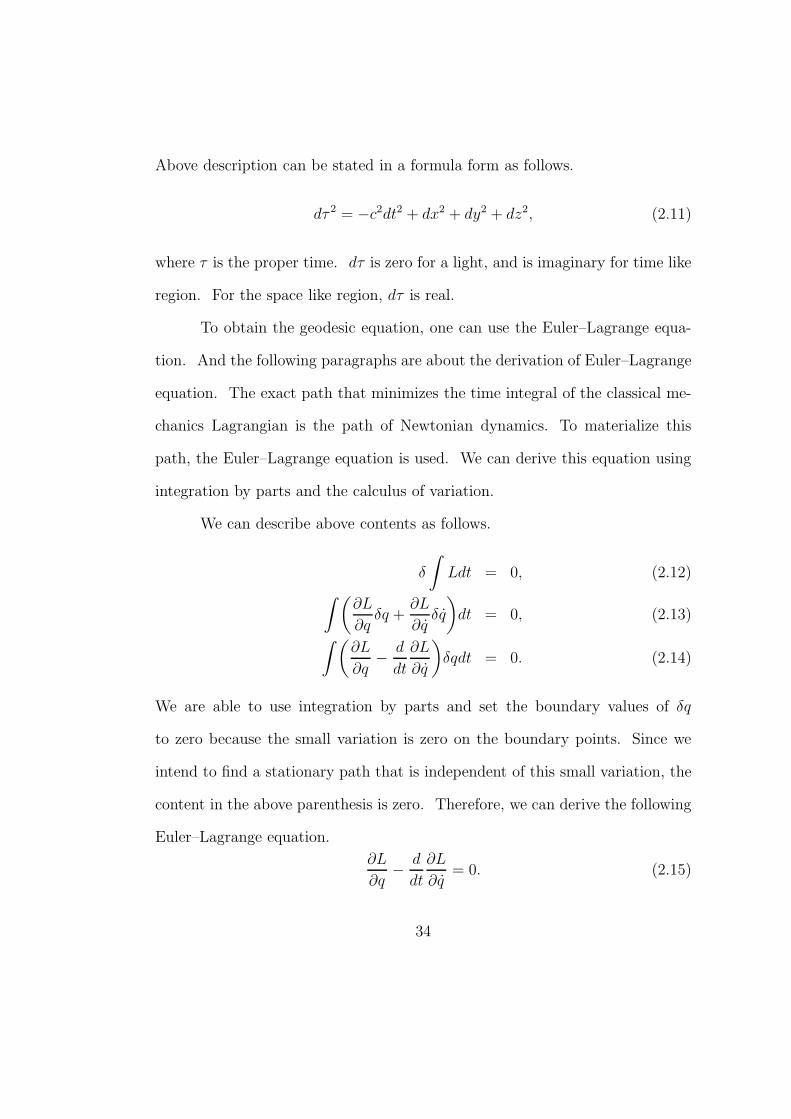
Above description can be stated in a formula form as follows.

dτ 2 = −c2dt2 + dx2 + dy2 + dz2, (2.11)

where τ is the proper time. dτ is zero for a light, and is imaginary for time like

region. For the space like region, dτ is real.

To obtain the geodesic equation, one can use the Euler–Lagrange equa-

tion. And the following paragraphs are about the derivation of Euler–Lagrange

equation. The exact path that minimizes the time integral of the classical me-

chanics Lagrangian is the path of Newtonian dynamics. To materialize this

path, the Euler–Lagrange equation is used. We can derive this equation using

integration by parts and the calculus of variation.

We can describe above contents as follows.

δ

∫

Ldt = 0, (2.12)

∫ (

∂L

∂qδq +

∂L

∂qδq

)

dt = 0, (2.13)

∫(

∂L

∂q− d

dt

∂L

∂q

)

δqdt = 0. (2.14)

We are able to use integration by parts and set the boundary values of δq

to zero because the small variation is zero on the boundary points. Since we

intend to find a stationary path that is independent of this small variation, the

content in the above parenthesis is zero. Therefore, we can derive the following

Euler–Lagrange equation.

∂L

∂q− d

dt

∂L

∂q= 0. (2.15)

34

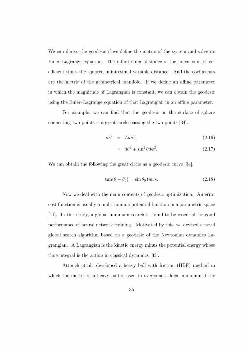
We can derive the geodesic if we define the metric of the system and solve its

Euler–Lagrange equation. The infinitesimal distance is the linear sum of co-

efficient times the squared infinitesimal variable distance. And the coefficients

are the metric of the geometrical manifold. If we define an affine parameter

in which the magnitude of Lagrangian is constant, we can obtain the geodesic

using the Euler–Lagrange equation of that Lagrangian in an affine parameter.

For example, we can find that the geodesic on the surface of sphere

connecting two points is a great circle passing the two points [34].

ds2 = Ldσ2, (2.16)

= dθ2 + sin2 θdφ2. (2.17)

We can obtain the following the great circle as a geodesic curve [34].

tan(θ − θ0) = sin θ0 tan s. (2.18)

Now we deal with the main contents of geodesic optimization. An error

cost function is usually a multi-minima potential function in a parametric space

[11]. In this study, a global minimum search is found to be essential for good

performance of neural network training. Motivated by this, we devised a novel

global search algorithm based on a geodesic of the Newtonian dynamics La-

grangian. A Lagrangian is the kinetic energy minus the potential energy whose

time integral is the action in classical dynamics [33].

Attouch et al. developed a heavy ball with friction (HBF) method in

which the inertia of a heavy ball is used to overcome a local minimum if the

35

ball has sufficient kinetic energy [5]. If the minimum is global, the frictional

force damps the motion of the ball and the ball converges to a global minimum.

However, an appropriate damping coefficient has not been found [5]. As such,

the ball is required to be restarted several times to complete the global mini-

mum search. Therefore, finding an appropriate adaptive damping coefficient is

crucial for good performance of the HBF algorithm in a global minimum search.

Cabot contributed to stabilizing the HBF algorithm with a regularization term

[9]. Despite this, the need for a well-controlled damping coefficient remains.

A hint of this problem was obtained from Qian’s paper [38]. He pre-

sented the convergence condition of critically damped oscillators as a quadratic

potential by using approximate linear dynamics. If we extend this critically

damped oscillator to a multi-minima potential, we can formulate a novel effi-

cient global search algorithm. However, Qian’s learning rule uses a constant

damping coefficient such that the damping force always opposes the velocity.

We required an adaptive descent to stop the ball at a global minimum and

an adaptive ascent rule to move the ball above a local minimum if it is not a

global minimum. Therefore, the problem was finding an appropriate damping

coefficient that recognizes the global minimum.

After considerable research, we derived this adaptive damping coefficient

from the concept of a geodesic, which is the shortest path connecting two points

in a curved manifold. Edelman et al. [17] and Nishmori and Akaho [37] devel-

oped a geodesic formulation in the orthogonal constraint conditions and derived

a learning rule based on orthogonal group theory. However, their problem was

36

an image-processing problem, namely, independent component analysis (ICA)

[37]. In contrast to their orthogonal group theoretical approach, we used this

geodesic concept for Newtonian dynamics applicable to a heavy ball. Newton’s

second law is obtained by minimizing the action, which is the time integral

of the classical Lagrangian. This is known as Hamilton’s principle in classical

mechanics [33]. However, our approach is to find the second-order equation

by minimizing the time integral of the square root of the Newtonian dynam-

ics Lagrangian. In this way, we obtained an adaptively damped second-order

equation whose convergence to a global minimum is guaranteed by the singular

crashing behavior of the heavy ball in an affine parameter coordinate. This

affine parameter was introduced to define a new Lagrangian whose value is con-

stant, as in ordinary differential geometry, to find the shortest curve connecting

the two points on a sphere [34].

We discretized the second-order rule obtained to derive a first-order adap-

tive steepest descent using the procedure presented in Qian’s paper [38]. Fur-

ther, we attempted to solve Rosenbrock- and Griewank-type potentials that were

used as examples in Attouch et al. [5]. Our adaptive learning rule exhibited

good performance for global minimization in these problems and we anticipate

that it will be applied to neural networks, economics, and game theory. Note

that our rule is valid only when the global minimum value is zero. This condi-

tion is necessary to produce a singularity in an affine parameter coordinate to

guarantee the convergence of a heavy ball.

37

2.3.2 Application

To test the validness of an adaptive steepest descent rule, we used Rosenbrock

and Griewank potentials. Rosenbrock potential is characterized by shallow val-

ley leading to a minimum site. Attouch et al. found that the heavy ball with

friction (HBF) method varies from underdamped to overdamped with an in-

crease of the damping constant [5]. Nevertheless, our adaptive damping coeffi-

cient found minimum site so easily and naturally. And the damping coefficient

was the negative time derivative of the logarithmic function of the potential.

Griewank potential consists of many local minima arising from the product of

sinusoid functions. A global minimum is located at the center because of the

well shaped term is added to the sinusoid term.

In Attouch et al.’s paper, HBF model explores the local minima instead of

searching the global minimum. They arrive at each local minimum then shoot

again from an appropriate position on the path in Griewank potential. But

our adaptive steepest descent finds the global minimum at once within twenty

initial conditions out of twenty one. The one failure was observed but the heavy

ball found the global minimum after the mass was increased. We may suppose

that this phenomenon was due to the increase of the inertia and an adaptive

damping term’s contribution for escaping from a local minimum.

38

2.3.3 Further Study

We can estimate the charge distribution on a conducting disk with an adaptive

steepest descent. A new potential is defined by the sum of the square of each

force at each radius. The number of the discrete radii is ten and these ten radii

are separated by equal distance. We made a hypothesis that the charges can

exist only on these discrete radii. We defined the weight coordinates by each

charge density on these ten radii. If the potential is zero then it means that ten

forces are all zero. Therefore this condition satisfies the zero force condition of

a charge on a conducting surface.

We searched the weight coordinate where the heavy ball stops, and com-

pared resulting coordinate with the analytic solution. Each weight coordinate

value is the charge density at each radius. The charge density increases with

the radius, and the increase pattern of HBF was similar to that of an analytic

solution. We supposed the error was due to the hypothesis that the charge

should exist on each discrete radii separated equally. Instead of this discrete

case, an analytic solution assumes that the charge can be anywhere on a disk.

2.4 Comparison of Two Algorithms

The comparison of stochastic and deterministic search algorithms are shown in

Table 2.3

39

Table 2.3: Comparison of two strategiesEvolutionary Optimization Geodesic Optimization

Subject Population of DNAmolecules

Heavy ball rolling on a po-tential

Aim of Optimization Minimizing the total Gibbsfree energy and maximiz-ing the number of target ds-DNA

Searching for the globalminimum in a multi-minimapotential

Dynamics Rule Population based randomsearch (variation) andMetropolis selection (selec-tion). Driving the systeminto the minimum Gibbsfree energy state by slowcooling

A geodesic of classicaldynamics Lagrangianδ∫ √

Lcdt = 0

Informational Fucntion Logical theorem proving Estimation of charge den-sity on a conducting disk

Style of Optimization Stochastic and Evolution-ary

Deterministic

40

Chapter 3

An Evolutionary Monte Carlo

Algorithm for Predicting DNA

Hybridization

3.1 DNA Computing

3.1.1 DNA Computing in General

Using the standard biochemistry lab techniques, we can solve the problems of

computer science, such as, the directed Hamiltonian path problem, DNA drug

design, chess game, and the tic-tac-toe game. These standard lab techniques

include PCR (polymerase chain reaction) for duplicating ssDNA, restriction

enzyme for cutting specific pattern of DNA base site, electrophoresis for sorting

41

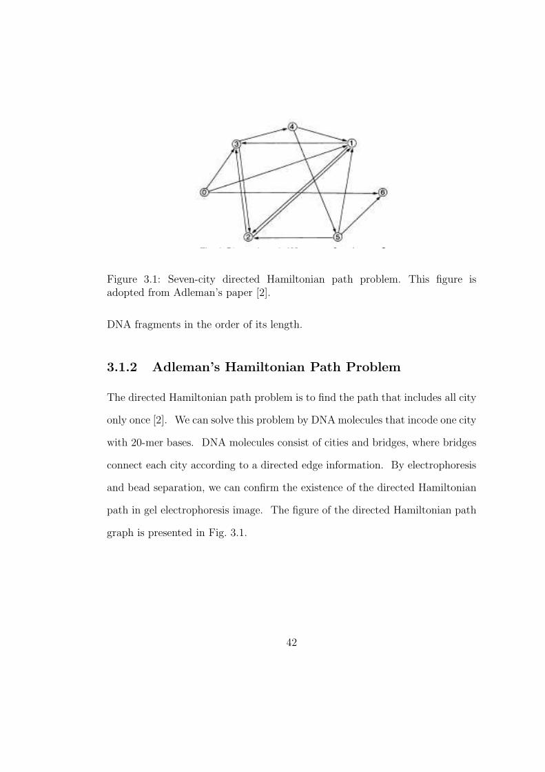
Figure 3.1: Seven-city directed Hamiltonian path problem. This figure isadopted from Adleman’s paper [2].

DNA fragments in the order of its length.

3.1.2 Adleman’s Hamiltonian Path Problem

The directed Hamiltonian path problem is to find the path that includes all city

only once [2]. We can solve this problem by DNA molecules that incode one city

with 20-mer bases. DNA molecules consist of cities and bridges, where bridges

connect each city according to a directed edge information. By electrophoresis

and bead separation, we can confirm the existence of the directed Hamiltonian

path in gel electrophoresis image. The figure of the directed Hamiltonian path

graph is presented in Fig. 3.1.

42

3.1.3 Benenson et al.’s in vitro Cancer Drug Design

With the restriction enzyme method, we can diagnoses the lung cancer and re-

lease the ssDNA drug in molecular automata framework [6]. A various restric-

tion enzymes cut the diagnosis part then the drug is released. The released drug

is supposed to suppress the gene expression of lung cancer. This experiment is

performed in vitro not in vivo. In other words, experiment was performed only

in test tube but not in human body.

3.1.4 “Knight Problem” in 3×3 Chess Board

The problem is to find the configuration of knights in 3×3 board on the condition

that each knight does not attack others. This problem can be transformed into

SAT problem and solved by mix and divide strategy of test tube [20].

3.1.5 “Tic-Tac-Toe” by Deoxyribozyme Based Automa-

tion

In this game, the winner is one who occupies three neighboring sites in straight

way. This game is implemented by deoxyribozyme which emit fluorescence on

the logic conditions, such as, “AND”, “OR”, and “NOR”. The molecular com-

puter does not lose the game because each 3 × 3 well contains the molecules

that were prepared for all possible path of evolution of game [46].

43

3.2 Evolutionary Monte Carlo Method

The physical objects in the simulation of reacting DNA molecules ssDNAs.

Each ssDNA has a base sequence designed for a given purpose, for example, the

theorem proving which was described in previous Chapter. We assume that all

the DNAs are in thermal equilibrium with the temperature T .

The important thermodynamic quantity in the following algorithm is

Gibbs free energy, which is defined by

G = Hb − TSu, (3.1)

where Hb is the total binding energy which is negative and Su is the entropy

of unbound base pairs which is positive. So, the Boltzmann probability for

the system to be in a particular state C is given by 1Ze−G(C)/kBT , where Z ≡

∑

C e−G(C)/kBT and kB is the Boltzmann constant.

Let us consider both the high temperature and the low temperature lim-

its. If the temperature is very high, all ssDNAs will be unbound because the

entropy term in Gibbs free energy is very large. If the system is at a low temper-

ature, the ssDNAs will form dsDNAs because the binding energy term in Gibbs

free energy becomes large in negative and the entropy term becomes negligible.

Therefore, assembling ssDNAs into a dsDNA or disassembling a dsDNA

into the original ssDNAs will be determined by the thermodynamics of the

binding energy term and the entropy term in Gibbs free energy.

The evolutionary Monte Carlo algorithm proceeds as follows.

(i) We start with an initial configuration of N ssDNAs with m types at a

44

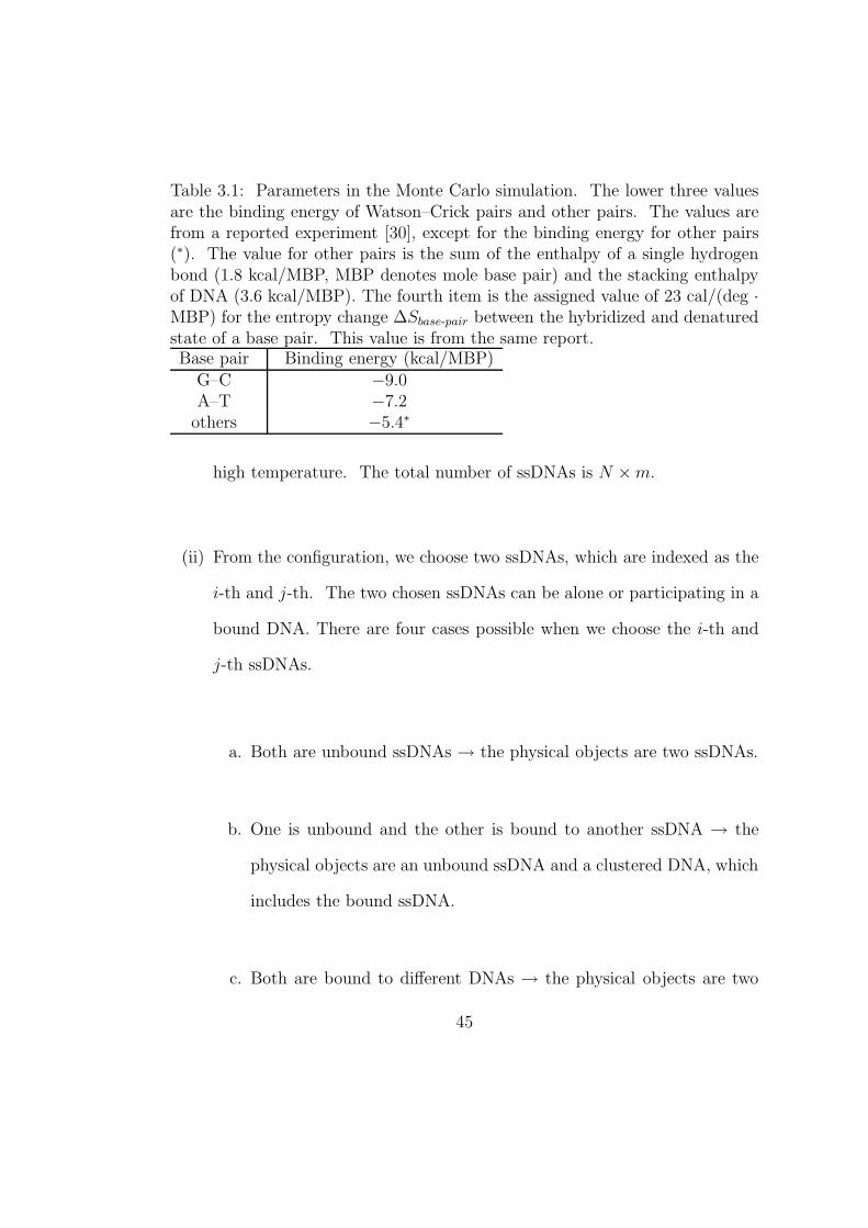
Table 3.1: Parameters in the Monte Carlo simulation. The lower three valuesare the binding energy of Watson–Crick pairs and other pairs. The values arefrom a reported experiment [30], except for the binding energy for other pairs(∗). The value for other pairs is the sum of the enthalpy of a single hydrogenbond (1.8 kcal/MBP, MBP denotes mole base pair) and the stacking enthalpyof DNA (3.6 kcal/MBP). The fourth item is the assigned value of 23 cal/(deg ·MBP) for the entropy change ∆Sbase-pair between the hybridized and denaturedstate of a base pair. This value is from the same report.Base pair Binding energy (kcal/MBP)

G–C −9.0A–T −7.2

others −5.4∗

high temperature. The total number of ssDNAs is N × m.

(ii) From the configuration, we choose two ssDNAs, which are indexed as the

i-th and j-th. The two chosen ssDNAs can be alone or participating in a

bound DNA. There are four cases possible when we choose the i-th and

j-th ssDNAs.

a. Both are unbound ssDNAs → the physical objects are two ssDNAs.

b. One is unbound and the other is bound to another ssDNA → the

physical objects are an unbound ssDNA and a clustered DNA, which

includes the bound ssDNA.

c. Both are bound to different DNAs → the physical objects are two

45

clusters, each of which includes each of the bound ssDNAs.

d. Both are bound together with (or without) ssDNAs → the physical

object is one cluster that includes the i-th and j-th ssDNAs.

(iii) We find out all possible M ways of binding the selected physical object(s).

(iv) We choose one of all possible M ways of binding. Here, we choose a

binding configuration with equal probability. This procedure corresponds

to a population-based evolutionary search. If this choice is accepted in

Metropolis selection in the next step, offspring molecules will be produced

in the hybridization process, which mimics the evolution of DNAs.

(v) We calculate the acceptance probability A with

A = min{1, e−∆G

kBT }, (3.2)

where ∆G ≡ G(C ′) − G(C), C ′ is the new configuration, and C is the

current configuration [35].

When two ssDNAs form a dsDNA, we can calculate ∆G as

∆G = ∆H − T∆S. (3.3)

46

The ∆H can be calculated easily as it sums the binding energies of A–T

and G–C pairs and the binding energies of other pairs (see Table 3.1).

The entropy is reduced when the pairs are formed; therefore, we use the

same entropy change for any possible pair because we want to make our

model as minimal as possible. In short, we have only four parameters

(Table 3.1 and its caption) in our model.

(vi) If the hybridization process is not chosen, we attempt a denaturation pro-

cess. We consider a new configuration where i or j is separated from one

of its bound strands. The probability of acceptance is given in Eq. (3.2).

(vii) We repeat (ii)–(vi) until the system reaches its thermal equilibrium and

then count the number of target DNAs and the number of base pairs

bound together.

(viii) We decrease the temperature by an appropriate amount and repeat (ii)–

(vii). The amount of variation in temperature should be small enough to

satisfy the annealing condition in a real experiment.

Note that we use simulated annealing in step (viii). This method is de-

signed for optimizing combinatorial problems [29]. If we cool the system slowly

47

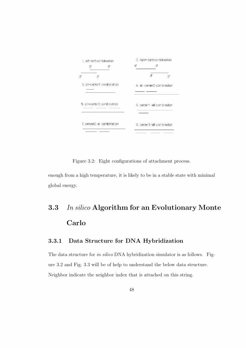
Figure 3.2: Eight configurations of attachment process.

enough from a high temperature, it is likely to be in a stable state with minimal

global energy.

3.3 In silico Algorithm for an Evolutionary Monte

Carlo

3.3.1 Data Structure for DNA Hybridization

The data structure for in silico DNA hybridization simulator is as follows. Fig-

ure 3.2 and Fig. 3.3 will be of help to understand the below data structure.

Neighbor indicate the neighbor index that is attached on this string.

48

3’ 5’

[0][0] [0][1] [2][0] [2][1] [3][0] [3][1]free site:

bound site[1][0] [1][1][7][0] [7][1] [8][0] [8][1]

Figure 3.3: Example of a data structure. And “mat” is omitted for each [][].

neighbor[0] is the left neighbor.

neighbor[1] is the right neighbor.

neighbor[2] is the first center neighbor.

neighbor[3] is the second center neighbor.

neighbor[4] is the third center neighbor.

mat[][] is the array for the information of free sites and bound sites.

mat[][0] is the first location.

mat[][1] is the last location.

mat[][0] == mat[][1] means that there is no space in it.

mat[0] : left free site.

mat[1] : right free site.

mat[2] : center1 free site.



mat[5] : left bound site.

mat[6] : right bound site.

49

mat[7] : center1 bound site.



3.3.2 Attaching Process

Calculate all possible combinations of eight kinds and choose one attaching pro-

cess randomly. The last choice is for the detaching process.

for(int i=0; i<10; i++)

totalfree += free[i];

selectedfree = (int)(1.0*rand()*totalfree/(RANDMAX+1.0));

//reactionpoint : the exact position in binding of selected type.

int reactionpoint = tempfree+free[j]-selectedfree;

//range of reactionpoint : (1 ∼ free[j])

//+——-tempfree——–+——free[j]———————+-free[j+1]-+

//+——+———-+——+———————————-+———–+

//+—selectedfree1——-+–reactionpoint-+-selectedfree2-+———–+

3.3.3 Detaching Process

We choose two ssDNAs or its cluster with randomness. Then calculate all possi-

ble combinations of them. After that process, we choose randomly one assembly

50

of all. There is also one chance to detach the chosen ssDNA from one of its

neighbor in its cluster.

3.4 Simulation Results for Theorem Proving

In this section, we describe a theorem proving problem using DNA molecules and

show the simulation results with the algorithm developed in previous sections.

Given a set of axioms, the objective of theorem proving is to show that a

statement is true. Basically, our logical inference is made by resolution refuta-

tion [36, 31]. In our work, five axioms are given as ¬Q∨¬P ∨R, Q∨¬T ∨¬S,

S, T , P , which are true, and the sentence to be proved is R.

Because we are interested in the consistency of R with the given axioms,

we use the proof by refutation method. First, we negate the R as ¬R. Then,

we make conjunction of the five axioms and ¬R. If we obtain nil, which is

always false, then we can say that ¬R is false and, finally, we can prove that R

is true.

We use the identity that (¬A ∨ B) ∧ A ≡ B when A is true. Also note

that, if A and B are true, then (A ∧ B) is true trivially. For example, let us

consider the operation of (Q∨¬T ∨¬S)∧S = Q∨¬T . Q∨¬T is true because

both Q ∨ ¬T ∨ ¬S and S are true. The statements obtained in each step in

Fig. 2.3 are all true and the last resolution with ¬R produces a contradiction.

So, we can conclude R is proved.

In molecular theorem proving, we use DNA molecules for representing

51

logical formulae and apply the hybridization of Watson–Crick complementary

pairs to the process of resolution refutation. Six sentences are encoded in syn-

thetic DNAs and their sequences are shown in Table 2.1. In Fig. 2.4, we show

the structure of the target dsDNA, which is nil in Fig. 2.3. If we obtain the

target dsDNA, we have proven that the theorem is true. Table 2.1 and Fig. 2.4

are adopted from Lee et al. with the permission of authors [31].

We simulated the DNA reaction process for theorem proving on a silicon-

based computer. First, we built the population of the six types of strands shown

in Table 2.1. Simulations were performed for 300, 600, and 900 molecules for

each sequence. The temperature was decreased from 95°C to 1°C by 1°C and

for each decrease in temperature, 108 reaction trials were made.

The simulation results are shown in Figs. 3.4 and 3.5. In Fig. 3.4, we

show the total number of pairs of A–T, G–C, and other pairs as a function of

temperature. Each curve stands for the data for N = 300, 600, and 900, where

N is the number of ssDNAs for each species. In this figure, we found that the

bonds begin to form at around 80°C and the number of bonds saturates at

around 50°C. This simulation result is consistent with the wet-lab experimental

result in the next section.

Fig. 3.5 shows the number of target dsDNAs as a function of temperature.

This data is important because it is the solution to the theorem proving problem.

We find that the target dsDNAs begin to form at around 63°C and the number

saturates at around 45°C. Note that this result is very hard to obtain in wet-lab

experiments, which implies that our estimation predicts the number of target

52

0

10000

20000

30000

40000

50000

60000

70000

30 40 50 60 70 80 90 100

Nu

mb

er

of

Bo

nd

s

Temperature(°C)

N=300N=600N=900

Figure 3.4: Simulation result of the number of bonds as a function of tempera-ture for N = 300, 600, and 900, where N is the number of ssDNA of each type.The pairing of bonds started to occur around 80°C and saturated at around50°C.

53

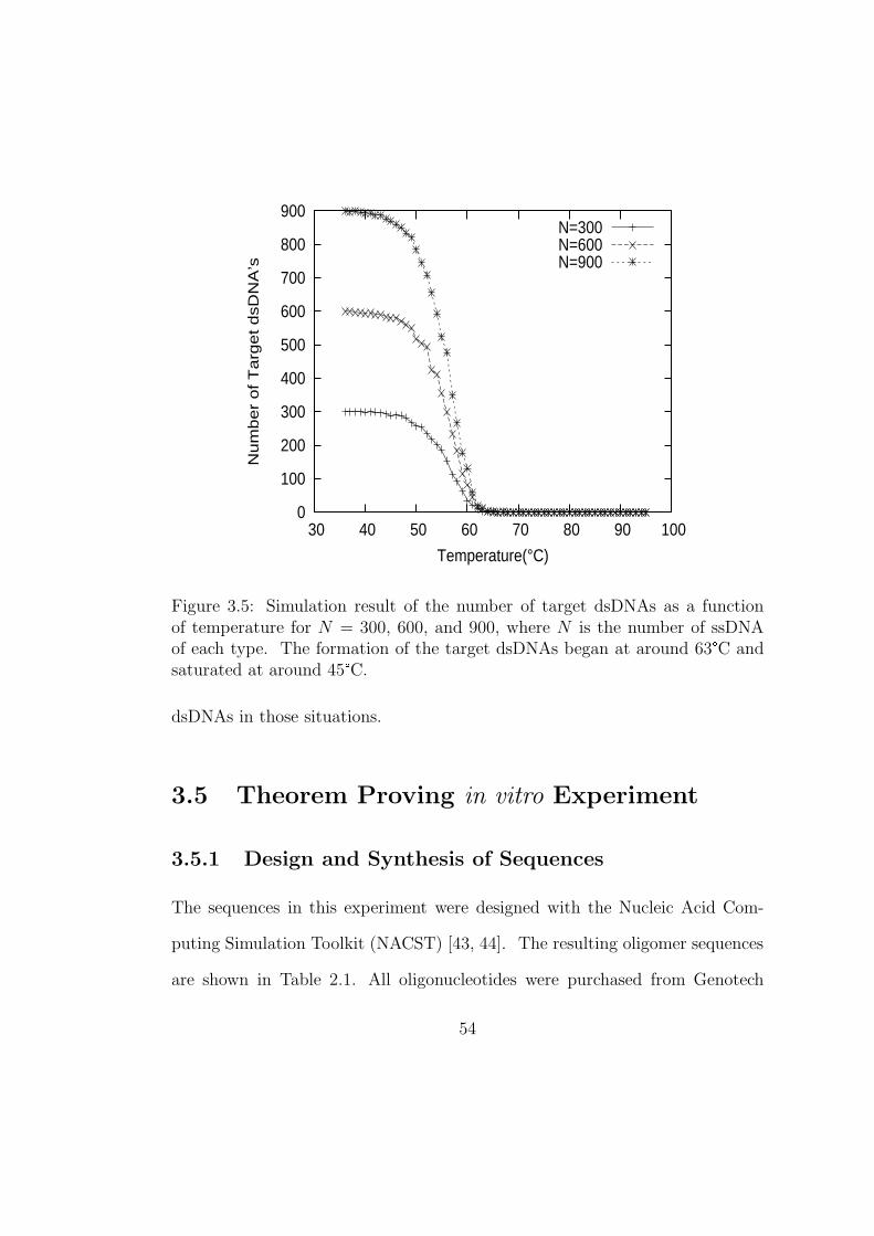
0

100

200

300

400

500

600

700

800

900

30 40 50 60 70 80 90 100

Nu

mb

er

of

Ta

rge

t d

sD

NA

’s

Temperature(°C)

N=300N=600N=900

Figure 3.5: Simulation result of the number of target dsDNAs as a functionof temperature for N = 300, 600, and 900, where N is the number of ssDNAof each type. The formation of the target dsDNAs began at around 63°C andsaturated at around 45°C.

dsDNAs in those situations.

3.5 Theorem Proving in vitro Experiment

3.5.1 Design and Synthesis of Sequences

The sequences in this experiment were designed with the Nucleic Acid Com-

puting Simulation Toolkit (NACST) [43, 44]. The resulting oligomer sequences

are shown in Table 2.1. All oligonucleotides were purchased from Genotech

54

(Bioneer, Korea). Each sequence pellet was brought to a stock concentration

100 pmol/µl in TE buffer (10 mM Tris-HCl, 1 mM EDTA, pH 8.0) and stored

at −20°C until its use.

3.5.2 Quantitative Annealing of Oligonucleotides

All six single strands were adjusted to 15 pmol (2× : 30 pmol, 3× : 45 pmol)

in a final volume of 20 µl . The ratio of DNA to IQ SYBR Green supermix (100

mM KCl, 40 mM Tris-HCl, pH 8.4, 0.4 mM each dNTP, 50 U/ml iTaq DNA

polymerase, 6 mM MgCl2, SYBR Green I, 20 nM fluorescein) in the reaction was

1:1 (by volume). The hybridization buffer was 1 M NaCl solution. The sample

was maintained at 95°C for 5 min and temperature annealing was performed as

we cooled the sample slowly to 5°C using iCycler (Bio-Rad, USA). The cooling

rate of annealing was 1°C/10 min. All reactions were performed in triplicate

with independent sample preparation, and technical repeats were carried out at

least twice in each reaction.

3.5.3 Visualization of the Hybridized Mixture by Elec-

trophoresis

The hybridized mixture was electrophoresised on a 12% Polyacrylamide gel.

The running buffer consisted of 0.045 M Tris-borate and 0.001 M EDTA (pH

8.0) (TBE). Gels were run on a Mini Polyacrylamide Gel System (Bio-rad)

for 150 min at 80 V with constant voltage. To define the molecular size of

55

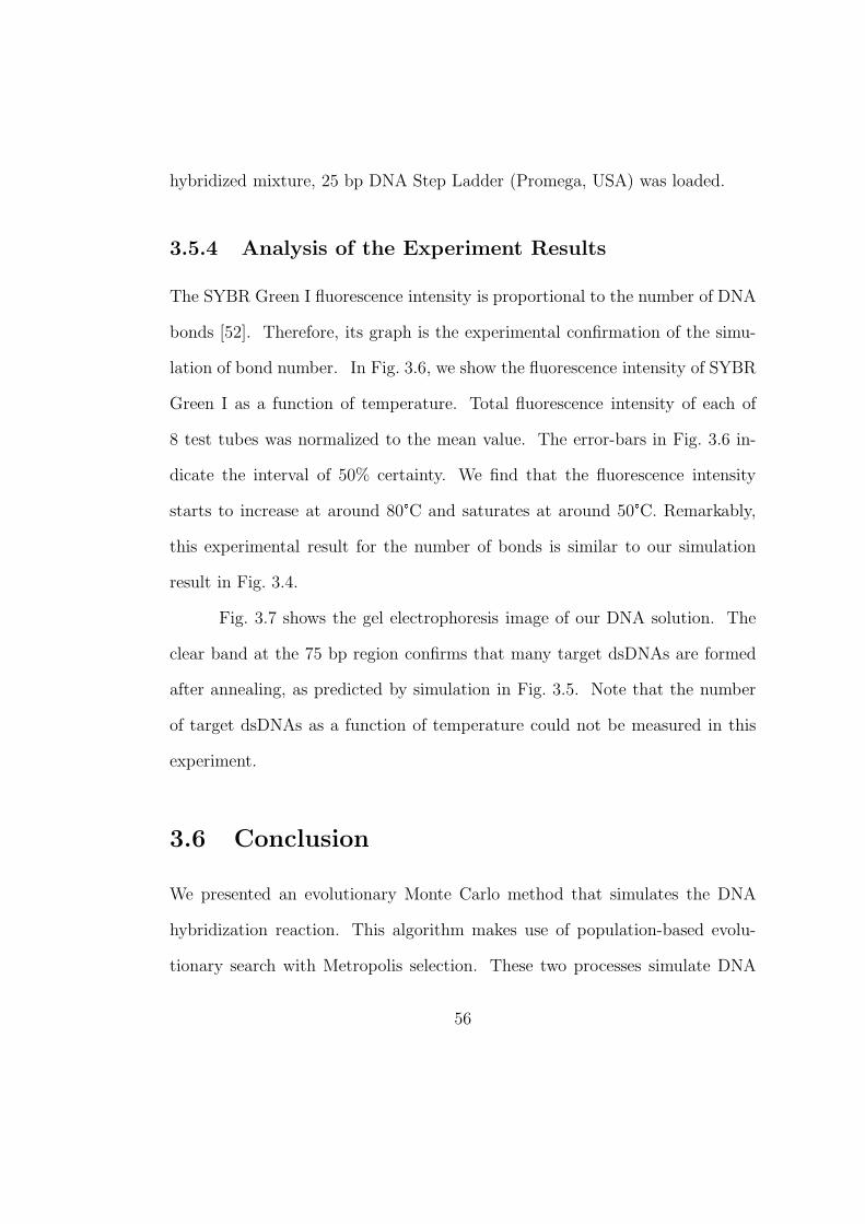
hybridized mixture, 25 bp DNA Step Ladder (Promega, USA) was loaded.

3.5.4 Analysis of the Experiment Results

The SYBR Green I fluorescence intensity is proportional to the number of DNA

bonds [52]. Therefore, its graph is the experimental confirmation of the simu-

lation of bond number. In Fig. 3.6, we show the fluorescence intensity of SYBR

Green I as a function of temperature. Total fluorescence intensity of each of

8 test tubes was normalized to the mean value. The error-bars in Fig. 3.6 in-

dicate the interval of 50% certainty. We find that the fluorescence intensity

starts to increase at around 80°C and saturates at around 50°C. Remarkably,

this experimental result for the number of bonds is similar to our simulation

result in Fig. 3.4.

Fig. 3.7 shows the gel electrophoresis image of our DNA solution. The

clear band at the 75 bp region confirms that many target dsDNAs are formed

after annealing, as predicted by simulation in Fig. 3.5. Note that the number

of target dsDNAs as a function of temperature could not be measured in this

experiment.

3.6 Conclusion

We presented an evolutionary Monte Carlo method that simulates the DNA

hybridization reaction. This algorithm makes use of population-based evolu-

tionary search with Metropolis selection. These two processes simulate DNA

56

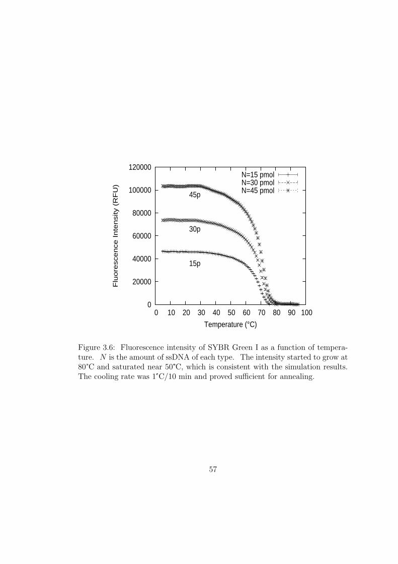
0

20000

40000

60000

80000

100000

120000

0 10 20 30 40 50 60 70 80 90 100

Flu

ore

sce

nce

In

ten

sity (

RF

U)

Temperature (°C)

15p

30p

45p

N=15 pmolN=30 pmolN=45 pmol

Figure 3.6: Fluorescence intensity of SYBR Green I as a function of tempera-ture. N is the amount of ssDNA of each type. The intensity started to grow at80°C and saturated near 50°C, which is consistent with the simulation results.The cooling rate was 1°C/10 min and proved sufficient for annealing.

57

Figure 3.7: Gel electrophoresis images of theorem proving DNA solutions afterannealing for 15, 30, and 45 pmol. Lane M shows the size marker, lane 1 shows45 pmol, lane 2 shows 30 pmol, and lane 3 shows 15 pmol ssDNA of each type.The brightness at 75 base pairs (bp) is proportional to the number of targetDNAs.

58

reactions in an evolutionary manner. The acceptance of a given reaction process

is determined by the Metropolis algorithm considering only four parameters of

enthalpy and entropy changes. Simulated annealing was used to keep the sys-

tem in the state of minimum Gibbs free energy as we lowered the temperature

slowly. With our evolutionary Monte Carlo algorithm, we obtained the numbers

of bonds as a function of temperature. The simulation results were consistent

with the subsequent experiments with synthesized DNA molecules designed for

solving the theorem proving problem. The number of target dsDNAs was ob-

tained as a function of temperature in the simulation, which was very hard to

obtain in the real DNA experiment. We obtained many target dsDNAs after

annealing in the simulation, which was confirmed by a clear band at the 75 bp

region in the gel electrophoresis image. The presence of this band showed that

the theorem was proved.

Of course, there will be issues in the practical use of our algorithm. First,

our algorithm does not prove general mathematical proofs such as Fermat’s last

theorem. The theorem proving in this work is a problem in artificial intelligence

adopting the resolution refutation [36, 31]. We clarify here that we perform

this kind of theorem proving by enumerating the number of target dsDNAs, i.e.

proofs, during the annealing process by taking possible combinations of state-

ments into account. Second, there may be DNA mismatches in the annealing

process. We would like to point out that we used DNA sequences of 15-mer

for each symbol which are designed to match correctly to avoid those possible

mismatches. For example, ¬Q ∨ ¬P ∨R is a single statement with three sym-

59

bols. Note that the length of 15-mer is longer than that of 10-mer of Adleman’s

Hamiltonian path problem [2] and is equal to that of 15-mer of the Knight prob-

lem [20]. Third, theorem proving with five axioms and one clause seems to be

easy when the number of statements is small. However, in other experiments,

they used around 10 statements. For example, Yang et al. applied a theorem

proving to medical diagnosis with microRNAs, DNAs, and gold nanoparticles

[50]. In this experiment, they used microRNAs as input data, DNAs as logic

elements, and the gold nanoparticles as display devices. Their number of state-

ments was ten. Also, the Winfree group implemented a 12 microRNA logic-gate

circuit [42]. This circuit was used for detecting gene expression patterns. Their

number of statements was twelve. Though our number of statements is around

half of those used in these experiments, we believe we can apply our algorithm

to more statements in future works.

In conclusion, we have shown that an evolutionary Monte Carlo can sim-

ulate the DNA hybridization process. The reliability of our algorithm was con-

firmed by a molecular biology experiment. This algorithm could be used in

modeling other DNA hybridization experiments with silicon-based computers.

60

Chapter 4

A Global Minimization

Algorithm Based on a Geodesic

of a Lagrangian Formulation of

Newtonian Dynamics

4.1 Derivation of an Adaptively Damped Os-

cillator

The Lagrangian for classical mechanics is defined as:

Lc =m

2

∑

1≤i≤n

(

dwi

dt

)2

− V, (4.1)

61

where m is the mass of the heavy ball; wi, the ith coordinate in a weight space; t,

time; and n, the dimension of a weight space. V is an error cost and is referred

to as the potential function in this paper. Solving the Euler–Lagrange equa-

tion using classical mechanics Lagrangian produces Newton’s second law, which

states that mass multiplied by acceleration is equal to the negative gradient of

a potential [33].

However, this classical dynamics Lagrangian is not constant, as is that

used for obtaining the geodesic of two points on a sphere [34]. Therefore, we

are interested in defining a new Lagrangian whose value is a constant over

time. This approach is similar to the geometrization of Newtonian dynamics in

defining the metric from the classical Newtonian Lagrangian [10]. The detailed

procedure is as:

ds2 = LNdσ2

= LCdt2

= −V dt2 +m

2

∑

1≤i≤n

dwi2, (4.2)

where σ is an affine parameter; ds, an infinitesimal distance in a manifold; LN ,

a new Lagrangian; and LC , a classical mechanics Lagrangian. Based on the

above relationship, we define LN as:

LN =1

2m

∑

1≤i≤n

(

dwi

dσ

)2

− V

(

dt

dσ

)2

. (4.3)

Our approach in defining a metric and obtaining a geodesic is similar to that

of the procedure in general relativity theory in that it considers both time and

62

weight as equivalent variables [34, 10]. By solving the Euler—Lagrange equa-

tion of LN , we obtain the following geodesic equations in the affine parameter

coordinate. The Euler–Lagrange equations are:

−∂LN

∂t+

d

dσ

∂LN

∂t= 0 (4.4)

and

−∂LN

∂wi+

d

dσ

∂LN

∂wi= 0, (4.5)

where the dot implies a derivative with respect to the affine parameter σ. Fur-

ther, they yield the following geodesic equations:

dt

dσ=

a

V, (4.6)

∂V

∂wi

(

a

V

)2

+d

dσ

(

mdwi

dσ

)

= 0, (4.7)

d2wi

dσ2= −ηa2 ∂

∂wi

(

− 1

V

)

, (4.8)

where a is a constant and η is the learning rate, which is equal to the reciprocal

of the mass, i.e., 1m

. The above equations are in affine parameter coordinates;

however, it is important to obtain the equation of motion in time t for the real

motion of a heavy ball. To change the variable from σ to t, we use the chain

rule:

dwi

dσ=

dt

dσ

dwi

dt, (4.9)

d2wi

dσ2=

dt

dσ

d

dt

(

dt

dσ

)

dwi

dt+

(

dt

dσ

)2d2wi

dt2. (4.10)

We can convert Eq. (4.8) into following form:

d2wi

dσ2= −ηa2

V 2

∂V

∂wi. (4.11)

63

Then we insert Eq. (4.10) into Eq. (4.11) with Eq. (4.6) as follows:

a

V

d

dt

(

a

V

)

dwi

dt+

a2

V 2

d2wi

dt2= −ηa2

V 2

∂V

∂wi. (4.12)

After multiplying Eq. (4.12) by V 2

a2 and arranging each term, we obtain Eq. (4.13).

d2wi

dt2=

d

dt(lnV )

dwi

dt− η

∂V

∂wi. (4.13)

4.2 Proof of Convergence to Global Minimum

with Zero Point Constraint

We obtained two geodesic equations in terms of the affine parameter (4.8) and

time (4.13). A geodesic equation in time t was derived from the geodesic equa-

tions in the affine parameter σ. We used the chain rule to change the indepen-

dent variable from t to σ.

In Eq. (4.8), the left hand side represents the acceleration and the right

hand side represents the force of a singular potential − 1V

. In Figure 4.1, we plot

V and − 1V

when the potential V = x2. Therefore, a mass will be accelerated

toward a weight coordinate, which satisfies V = 0, with an infinite speed in

an affine parameter coordinate because a negative inverse potential leads to

negative infinity at weights satisfying V = 0. If this mass crash were observed

in time, the mass would appear to accelerate toward an equilibrium weight

coordinate and then be decelerated by an adaptive damping force represented

by the first term on the right hand side of Eq. (4.13). Finally, if the minimum

value of the potential were zero, then the heavy ball would stop at the minimum

64

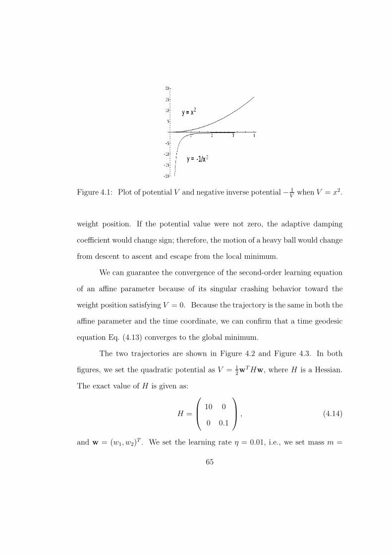
Figure 4.1: Plot of potential V and negative inverse potential − 1V

when V = x2.

weight position. If the potential value were not zero, the adaptive damping

coefficient would change sign; therefore, the motion of a heavy ball would change

from descent to ascent and escape from the local minimum.

We can guarantee the convergence of the second-order learning equation

of an affine parameter because of its singular crashing behavior toward the

weight position satisfying V = 0. Because the trajectory is the same in both the

affine parameter and the time coordinate, we can confirm that a time geodesic

equation Eq. (4.13) converges to the global minimum.

The two trajectories are shown in Figure 4.2 and Figure 4.3. In both

figures, we set the quadratic potential as V = 12wTHw, where H is a Hessian.

The exact value of H is given as:

H =

10 0

0 0.1

, (4.14)

and w = (w1, w2)T . We set the learning rate η = 0.01, i.e., we set mass m =

65

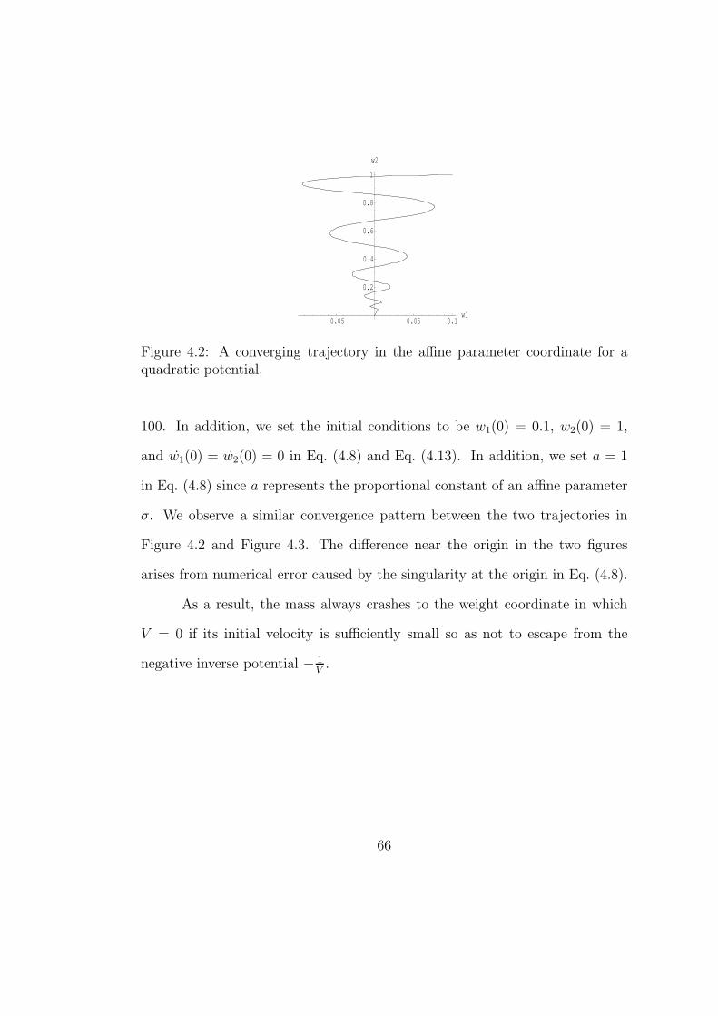
-0.05 0.05 0.1w1

0.2

0.4

0.6

0.8

1

w2

Figure 4.2: A converging trajectory in the affine parameter coordinate for aquadratic potential.

100. In addition, we set the initial conditions to be w1(0) = 0.1, w2(0) = 1,

and w1(0) = w2(0) = 0 in Eq. (4.8) and Eq. (4.13). In addition, we set a = 1

in Eq. (4.8) since a represents the proportional constant of an affine parameter

σ. We observe a similar convergence pattern between the two trajectories in

Figure 4.2 and Figure 4.3. The difference near the origin in the two figures

arises from numerical error caused by the singularity at the origin in Eq. (4.8).

As a result, the mass always crashes to the weight coordinate in which

V = 0 if its initial velocity is sufficiently small so as not to escape from the

negative inverse potential − 1V

.

66

-0.1 -0.05 0.05 0.1w1

0.2

0.4

0.6

0.8

1w2

Figure 4.3: A converging trajectory in time for a quadratic potential.

4.3 Derivation of a Novel Adaptive Steepest

Descent in a Discrete Time Case

In this section, we derive a novel steepest descent with adaptive momentum. We

refer to the procedure in Qian’s paper [38]. Qian derived the momentum term

and the learning rate in quadratic potential for a critically damped oscillator.

We discretize Eq. (4.13) as follows:

wt+∆t + wt−∆t − 2wt

(∆t)2=

lnVt − lnVt−∆t

∆t

wt+∆t −wt

∆t− 1

m

∂V

∂w. (4.15)

After rearranging the terms, we arrive at the first-order update rule, which is:

wt+∆t −wt =1

1 − (lnVt − lnVt−∆t)(wt − wt−∆t)

− (∆t)2

1 − (lnVt − lnVt−∆t)

1

m

∂V

∂w. (4.16)

The above learning rule is an adaptive steepest descent rule and m is the mass of

the particle, i.e., the reciprocal of learning rate η. We can compare our learning

67

rule with that from Qian’s paper [38] as follows:

wt+∆t −wt =m

m + µ∆t(wt −wt−∆t)

− (∆t)2

m + µ∆t

∂V

∂w, (4.17)

where µ is a damping constant; m, a particle’s mass; and the constant before

the gradient is the learning rate.

We can determine the fixed learning rate and momentum parameter in

Eq. (4.17), which are given as:

ηf =(∆t)2

m + µ∆t, (4.18)

pf =m

m + µ∆t, (4.19)

where ηf is the learning rate and pf is the momentum parameter in Qian’s paper

on a critically damped oscillator [38]. In addition, we can obtain adaptively the

learning rate ηa and the momentum parameter pa in Eq. (4.16), which are given

by:

ηa =(∆t)2

1 − (lnVt − lnVt−∆t)

1

m(4.20)

and

pa =1

1 − (lnVt − lnVt−∆t). (4.21)

Note that Qian’s steepest descent is optimal for a quadratic potential; however,

our adaptive steepest descent is applicable for a multiminima potential with a

zero global minimum value.

68

4.4 Examples of Global Optimization with Zero

Point Constraint

We applied the adaptive steepest descent obtained (4.16) to global minimum

search problems. We took two examples from Attouch et al.’s paper [5] for

a global minimum exploration. Mathematica 5.0 was used for the numerical

calculations.

First, we applied our adaptive steepest descent rule (4.16) to the Rosen-

brock potential. The exact form of the potential is as follows:

V (x, y) = 100(y − x2)2 + (1 − x)2, (4.22)

and the global minimum of the Rosenbrock potential is located at (1, 1). We

set the particle mass m = 1000 and time increment ∆t = 1. The initial two

points were set at (−1.2, 1). The global search result based on our rule (4.16)

is presented in Figure 4.4. We observe that the heavy ball arrives at the global

minimum at (1, 1) directly.

We observe that our method provides some control over the damping

coefficient to obtain a rapid oscillation-free trajectory, a feature that was absent

in Attouch et al. [5]. Their path depended on a damping coefficient. Higher

values of the damping coefficient were observed to generate slow trajectories

resembling those of steepest descent, whereas lower values generated rapid tra-

jectories with oscillations that grew as the coefficient decreased.

Second, we checked the convergence of the heavy ball in a Griewank-type

69

-1 -0.5 0 0.5 1

-1

-0.5

0

0.5

1

Figure 4.4: A global minimum search for the Rosenbrock potential. The twoinitial points are (−1.2, 1) and the global minimum is located at (1, 1). We ob-serve excellent convergence of a learning point to the global minimum. Particlemass m = 1000.

70

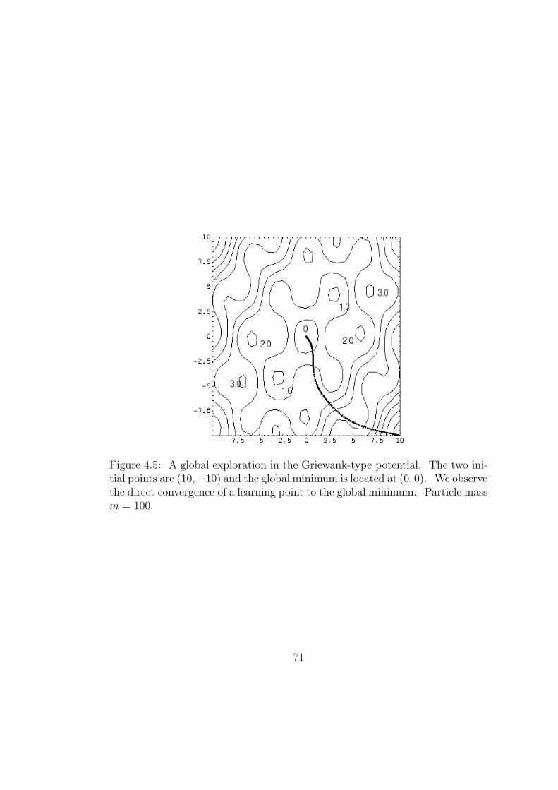
Figure 4.5: A global exploration in the Griewank-type potential. The two ini-tial points are (10,−10) and the global minimum is located at (0, 0). We observethe direct convergence of a learning point to the global minimum. Particle massm = 100.

71

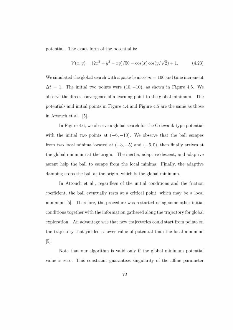
potential. The exact form of the potential is:

V (x, y) = (2x2 + y2 − xy)/50 − cos(x) cos(y/√

2) + 1. (4.23)

We simulated the global search with a particle mass m = 100 and time increment

∆t = 1. The initial two points were (10,−10), as shown in Figure 4.5. We

observe the direct convergence of a learning point to the global minimum. The

potentials and initial points in Figure 4.4 and Figure 4.5 are the same as those

in Attouch et al. [5].

In Figure 4.6, we observe a global search for the Griewank-type potential

with the initial two points at (−6,−10). We observe that the ball escapes

from two local minima located at (−3,−5) and (−6, 0), then finally arrives at

the global minimum at the origin. The inertia, adaptive descent, and adaptive

ascent help the ball to escape from the local minima. Finally, the adaptive

damping stops the ball at the origin, which is the global minimum.

In Attouch et al., regardless of the initial conditions and the friction

coefficient, the ball eventually rests at a critical point, which may be a local

minimum [5]. Therefore, the procedure was restarted using some other initial

conditions together with the information gathered along the trajectory for global

exploration. An advantage was that new trajectories could start from points on

the trajectory that yielded a lower value of potential than the local minimum

[5].

Note that our algorithm is valid only if the global minimum potential

value is zero. This constraint guarantees singularity of the affine parameter

72

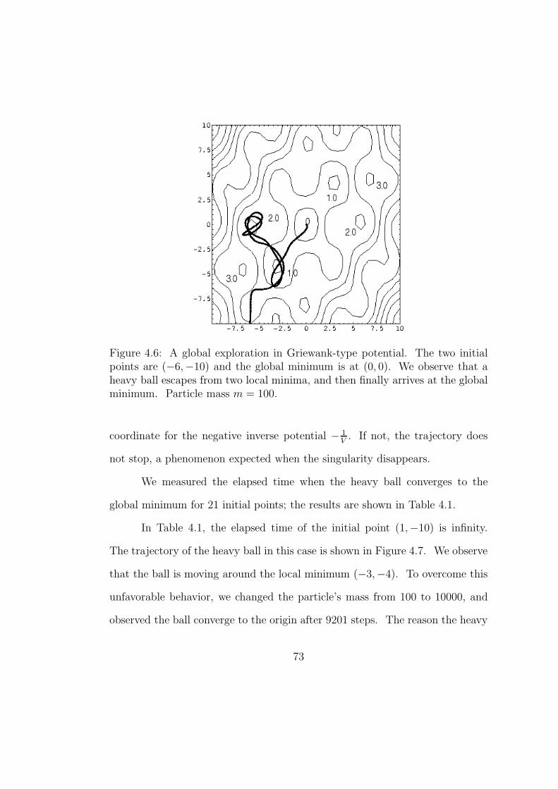
Figure 4.6: A global exploration in Griewank-type potential. The two initialpoints are (−6,−10) and the global minimum is at (0, 0). We observe that aheavy ball escapes from two local minima, and then finally arrives at the globalminimum. Particle mass m = 100.

coordinate for the negative inverse potential − 1V

. If not, the trajectory does

not stop, a phenomenon expected when the singularity disappears.

We measured the elapsed time when the heavy ball converges to the

global minimum for 21 initial points; the results are shown in Table 4.1.

In Table 4.1, the elapsed time of the initial point (1,−10) is infinity.

The trajectory of the heavy ball in this case is shown in Figure 4.7. We observe

that the ball is moving around the local minimum (−3,−4). To overcome this

unfavorable behavior, we changed the particle’s mass from 100 to 10000, and

observed the ball converge to the origin after 9201 steps. The reason the heavy

73

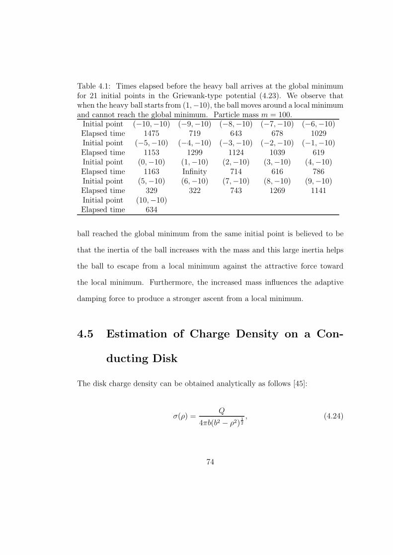
Table 4.1: Times elapsed before the heavy ball arrives at the global minimumfor 21 initial points in the Griewank-type potential (4.23). We observe thatwhen the heavy ball starts from (1,−10), the ball moves around a local minimumand cannot reach the global minimum. Particle mass m = 100.

Initial point (−10,−10) (−9,−10) (−8,−10) (−7,−10) (−6,−10)Elapsed time 1475 719 643 678 1029Initial point (−5,−10) (−4,−10) (−3,−10) (−2,−10) (−1,−10)Elapsed time 1153 1299 1124 1039 619Initial point (0,−10) (1,−10) (2,−10) (3,−10) (4,−10)Elapsed time 1163 Infinity 714 616 786Initial point (5,−10) (6,−10) (7,−10) (8,−10) (9,−10)Elapsed time 329 322 743 1269 1141Initial point (10,−10)Elapsed time 634

ball reached the global minimum from the same initial point is believed to be

that the inertia of the ball increases with the mass and this large inertia helps

the ball to escape from a local minimum against the attractive force toward

the local minimum. Furthermore, the increased mass influences the adaptive

damping force to produce a stronger ascent from a local minimum.

4.5 Estimation of Charge Density on a Con-

ducting Disk

The disk charge density can be obtained analytically as follows [45]:

σ(ρ) =Q

4πb(b2 − ρ2)12

, (4.24)

74

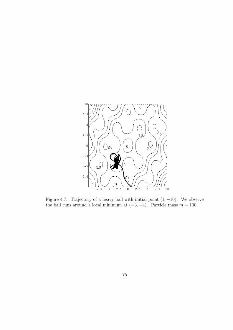
Figure 4.7: Trajectory of a heavy ball with initial point (1,−10). We observethe ball runs around a local minimum at (−3,−4). Particle mass m = 100.

75

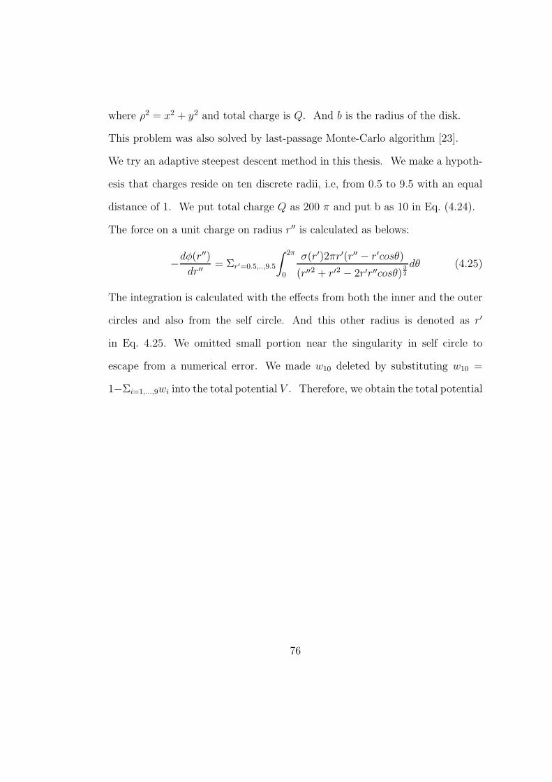
where ρ2 = x2 + y2 and total charge is Q. And b is the radius of the disk.

This problem was also solved by last-passage Monte-Carlo algorithm [23].

We try an adaptive steepest descent method in this thesis. We make a hypoth-

esis that charges reside on ten discrete radii, i.e, from 0.5 to 9.5 with an equal

distance of 1. We put total charge Q as 200 π and put b as 10 in Eq. (4.24).

The force on a unit charge on radius r′′ is calculated as belows:

−dφ(r′′)

dr′′= Σr′=0.5,..,9.5

∫

0

2π σ(r′)2πr′(r′′ − r′cosθ)

(r′′2 + r′2 − 2r′r′′cosθ)32

dθ (4.25)

The integration is calculated with the effects from both the inner and the outer

circles and also from the self circle. And this other radius is denoted as r′

in Eq. 4.25. We omitted small portion near the singularity in self circle to

escape from a numerical error. We made w10 deleted by substituting w10 =

1−Σi=1,...,9wi into the total potential V . Therefore, we obtain the total potential

76

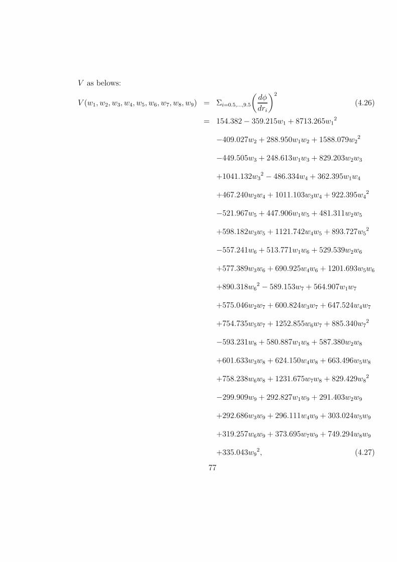
V as belows:

V (w1, w2, w3, w4, w5, w6, w7, w8, w9) = Σi=0.5,...,9.5

(

dφ

dri

)2

(4.26)

= 154.382 − 359.215w1 + 8713.265w12

−409.027w2 + 288.950w1w2 + 1588.079w22

−449.505w3 + 248.613w1w3 + 829.203w2w3

+1041.132w32 − 486.334w4 + 362.395w1w4

+467.240w2w4 + 1011.103w3w4 + 922.395w42

−521.967w5 + 447.906w1w5 + 481.311w2w5

+598.182w3w5 + 1121.742w4w5 + 893.727w52

−557.241w6 + 513.771w1w6 + 529.539w2w6

+577.389w3w6 + 690.925w4w6 + 1201.693w5w6

+890.318w62 − 589.153w7 + 564.907w1w7

+575.046w2w7 + 600.824w3w7 + 647.524w4w7

+754.735w5w7 + 1252.855w6w7 + 885.340w72

−593.231w8 + 580.887w1w8 + 587.380w2w8

+601.633w3w8 + 624.150w4w8 + 663.496w5w8

+758.238w6w8 + 1231.675w7w8 + 829.429w82

−299.909w9 + 292.827w1w9 + 291.403w2w9

+292.686w3w9 + 296.111w4w9 + 303.024w5w9

+319.257w6w9 + 373.695w7w9 + 749.294w8w9

+335.043w92, (4.27)

77

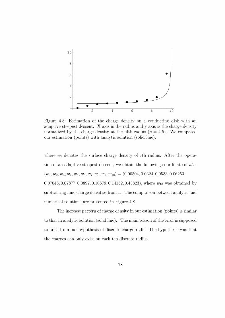
2 4 6 8 10

2

4

6

8

10

Figure 4.8: Estimation of the charge density on a conducting disk with anadaptive steepest descent. X axis is the radius and y axis is the charge densitynormalized by the charge density at the fifth radius (ρ = 4.5). We comparedour estimation (points) with analytic solution (solid line).

where wi denotes the surface charge density of ith radius. After the opera-

tion of an adaptive steepest descent, we obtain the following coordinate of w′s.

(w1, w2, w3, w4, w5, w6, w7, w8, w9, w10) = (0.00504, 0.0324, 0.0533, 0.06253,

0.07048, 0.07877, 0.0897, 0.10679, 0.14152, 0.43823), where w10 was obtained by

subtracting nine charge densities from 1. The comparison between analytic and

numerical solutions are presented in Figure 4.8.

The increase pattern of charge density in our estimation (points) is similar

to that in analytic solution (solid line). The main reason of the error is supposed

to arise from our hypothesis of discrete charge radii. The hypothesis was that

the charges can only exist on each ten discrete radius.

78

4.6 Conclusion

We have developed a novel algorithm for a global minimization based on the

HBF method. Our geodesic of Newtonian dynamics Lagrangian produced a

novel momentum parameter and learning rate. We confirmed the validity of

our learning rule by applying it to Rosenbrock- and Griewank-type potentials.

The most significant finding of this research is that we devised a mini-

mization rule for the global minimum search problem. The minimization rule

for Newtonian dynamics is Hamilton’s principle in which the time integral of the

Newtonian dynamics Lagrangian is minimized. Furthermore, in our rule, the

minimum search algorithm is obtained by minimizing the time integral of the

square root of the Newtonian dynamics Lagrangian. The difference between

the Newtonian dynamics rule and our optimization rule is whether we use the

Newtonian dynamics Lagrangian or its square root.

The second important finding is that an appropriate damping coefficient

for a damped oscillator equation for global minimization was determined. We

propose the negative time derivative of the logarithmic function of the error cost

as an adaptive damping coefficient. Finding this coefficient has been researched

since the study by Attouch et al. [9].

Finally, we can interpret the meaning of this work by implementing artifi-

cial intelligence based on the Newtonian dynamics rule. This mechanical mod-

eling provides us with a clear and easy understanding of the optimization by

using the physical concept of the HBF. This understanding is useful in simplify-

79

ing a complex problem and suggesting a most effective solution to this simplified

problem using mechanical optimization. The applicable cost functions will be

those of economics, game theory, and neural networks with a constraint on the

potential; namely, the global minimum value must be zero.

Future work aims to devise a novel adaptive algorithm that works without

these constraints. This includes developing a principle to change the potential

incrementally so that it can have a singularity for future moves.

80

Chapter 5

Conclusion

In Chapter 3, DNA fragments began to assemble at around 80°C in both in silico

and in vitro experiments. Target dsDNAs appeared at around 63°C in silicon-

based experiment. Most of the six kinds of DNA fragments were combined into

75-mer target dsDNAs in both in silico and in vitro experiments.

In Chapter 4, an adaptive Langevin equation, i.e. an adaptive steepest

descent, found the global minimum well on both Rosenbrock and Griewank po-

tentials. There was no large oscillation during the searching process on Rosen-

brock potential. For the Griewank potential, a heavy ball found the global min-

imum in twenty cases out of twenty one. The heavy ball with increased mass

found the global minimum from the previously failed initial condition with a

less massive ball.

In summary, we developed two optimization rules based on the physics.

Though the problems were artificial intelligence problem and electrostatic prob-

81

lem, the search methods were developed based on thermodynamics and differ-

ential geometry. We can see that interdisciplinary study provides good opti-

mization performance in this thesis. Therefore, it can be possible for physi-

cal principle to be used for machine learning, neural networks, and economics

problems. Physical modeling and mathematical approaches were found to be

effective in dealing with molecular theorem proving and global minimum search.

We also expect the contributions from neighboring research fields to physical

science with novel ideas to solve physical problems.

For the further study, DNA associative memory recall can be imple-

mented by a partial pattern matching of a query ssDNA with whole assembled

molecule. A biotin can be attached to a query DNA and a compound molecule

of the query and the answer can be attracted to the reading sector magnetically.

Also neural network problem can be solved with an adaptive Langevin

method. For example “XOR” problem can be solved by artificial neural net-

work. The potential energy can be the difference between the true value by an

oracle and the estimated value by the network. If the potential energy can be

expressed by the weights of whole synapses, then the heavy ball will stop at the

zero potential condition site.

Finally, Einstein field equation can be calculated for an adaptive Langevin

equation. Einstein field equation states that Einstein tensor which is obtained

from the metric equals to the energy momentum tensor. We can derive Ein-

stein tensor from the metric of classical mechanics Lagrangian and search for

the fundamental relation for optimization process as in the theory of general

82

relativity.

83

Appendix A

Trajectories of a Heavy Ball on

Griewank Potential from Initial

Points (−10,−10) to (10,−10).

84

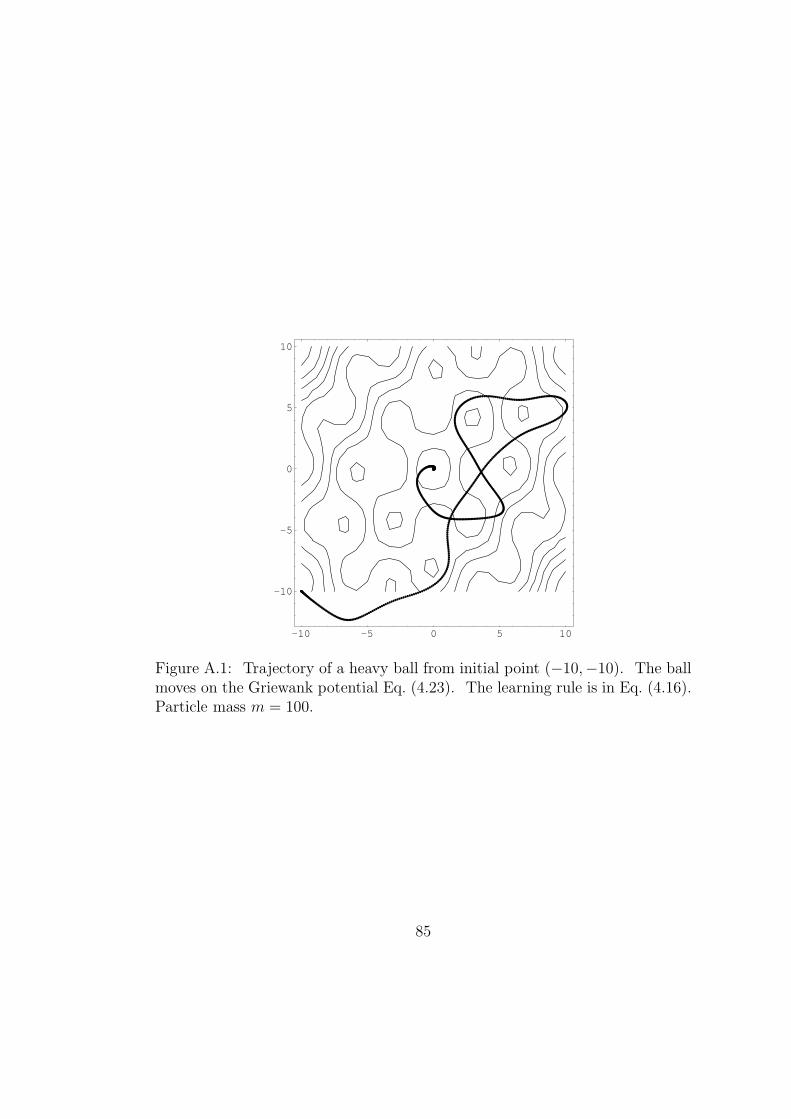
-10 -5 0 5 10

-10

-5

0

5

10

Figure A.1: Trajectory of a heavy ball from initial point (−10,−10). The ballmoves on the Griewank potential Eq. (4.23). The learning rule is in Eq. (4.16).Particle mass m = 100.

85

-10 -5 0 5 10

-10

-5

0

5

10


86

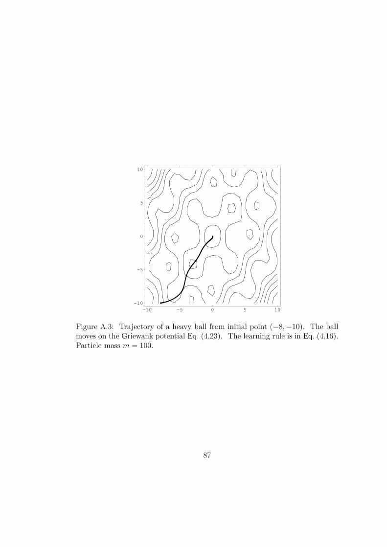
-10 -5 0 5 10-10

-5

0

5

10


87

-10 -5 0 5 10-10

-5

0

5

10


88

-10 -5 0 5 10-10

-5

0

5

10


89

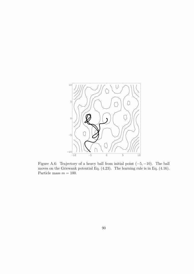
-10 -5 0 5 10-10

-5

0

5

10


90

-10 -5 0 5 10-10

-7.5

-5

-2.5

0

2.5

5


91

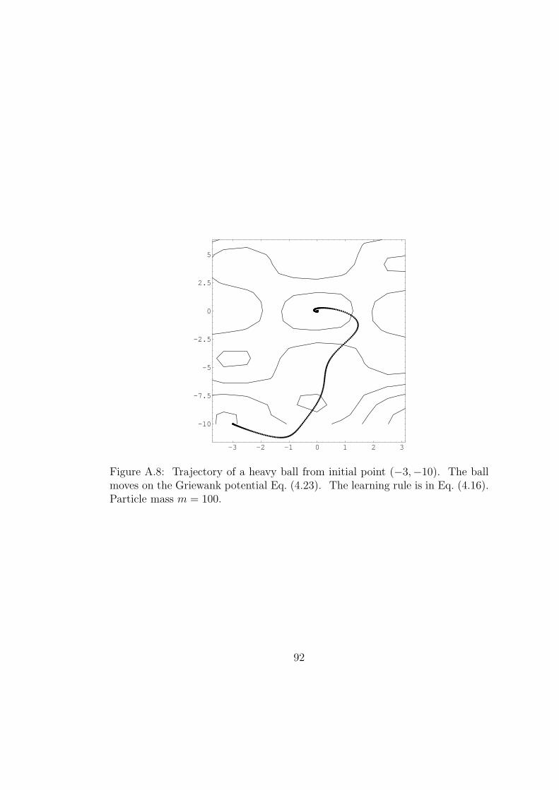
-3 -2 -1 0 1 2 3

-10

-7.5

-5

-2.5

0

2.5

5


92

-2 -1 0 1 2-10

-8

-6

-4

-2

0

2

4


93

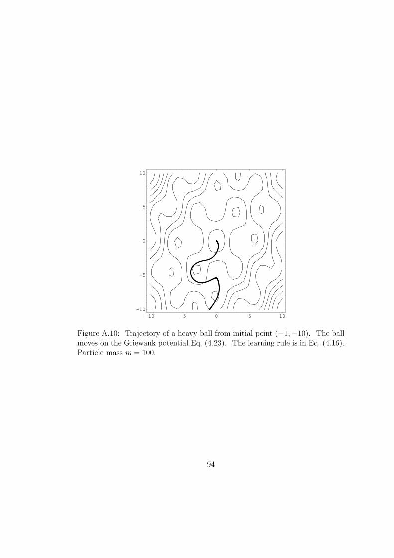
-10 -5 0 5 10-10

-5

0

5

10


94

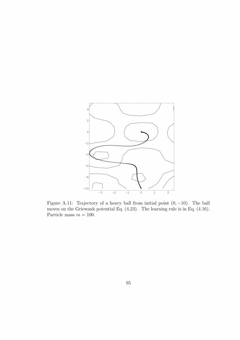
-3 -2 -1 0 1 2-10

-8

-6

-4

-2

0

2

4

Figure A.11: Trajectory of a heavy ball from initial point (0,−10). The ballmoves on the Griewank potential Eq. (4.23). The learning rule is in Eq. (4.16).Particle mass m = 100.

95

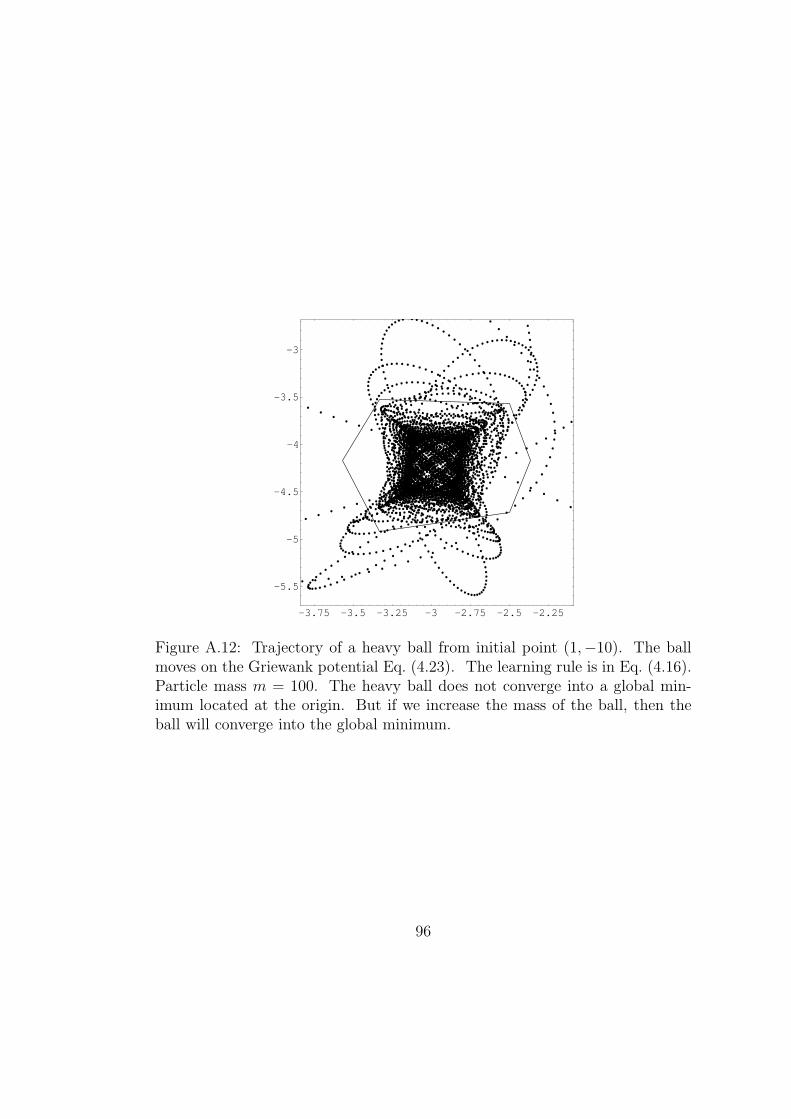
-3.75 -3.5 -3.25 -3 -2.75 -2.5 -2.25

-5.5

-5

-4.5

-4

-3.5

-3

Figure A.12: Trajectory of a heavy ball from initial point (1,−10). The ballmoves on the Griewank potential Eq. (4.23). The learning rule is in Eq. (4.16).Particle mass m = 100. The heavy ball does not converge into a global min-imum located at the origin. But if we increase the mass of the ball, then theball will converge into the global minimum.

96

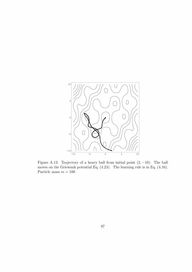
-10 -5 0 5 10-10

-5

0

5

10


97

-10 -5 0 5 10-10

-5

0

5

10


98

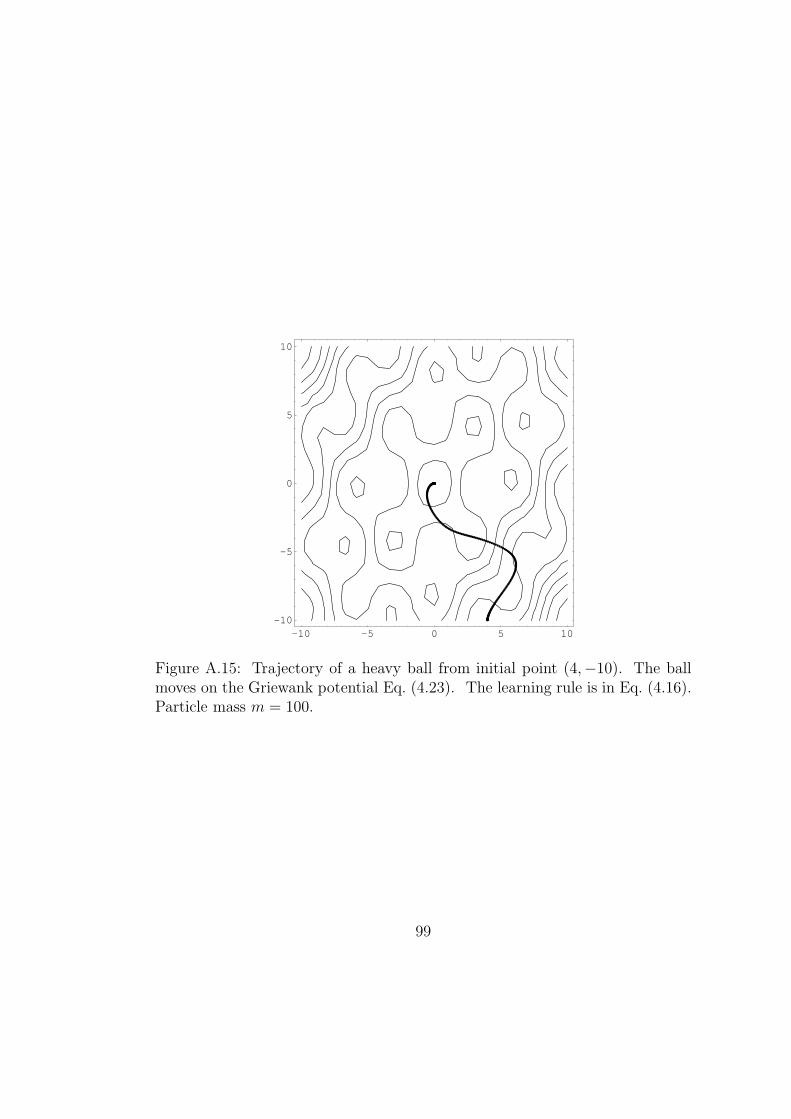
-10 -5 0 5 10-10

-5

0

5

10


99

-10 -5 0 5 10-10

-5

0

5

10


100

-10 -5 0 5 10-10

-5

0

5

10


101

-10 -5 0 5 10-10

-5

0

5

10


102

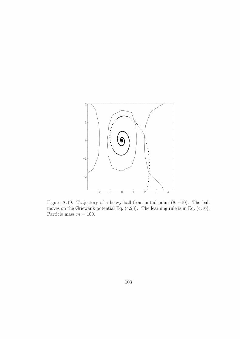
-2 -1 0 1 2 3 4

-2

-1

0

1

2


103

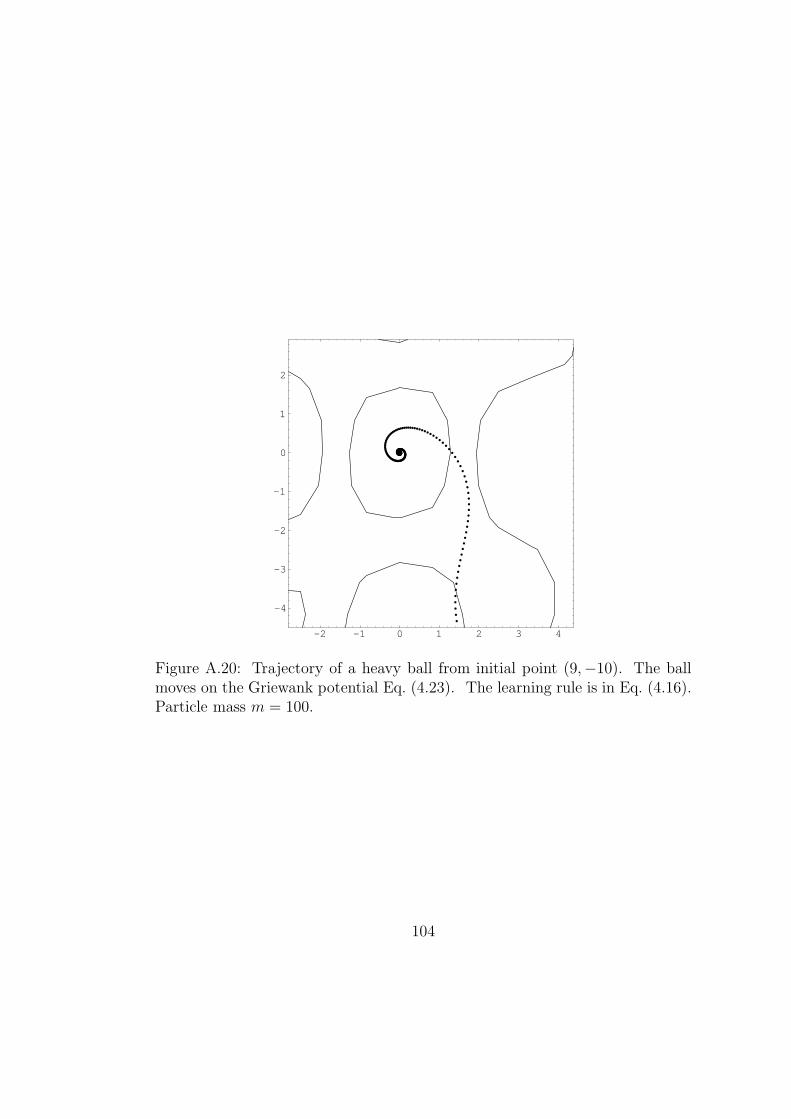
-2 -1 0 1 2 3 4

-4

-3

-2

-1

0

1

2


104

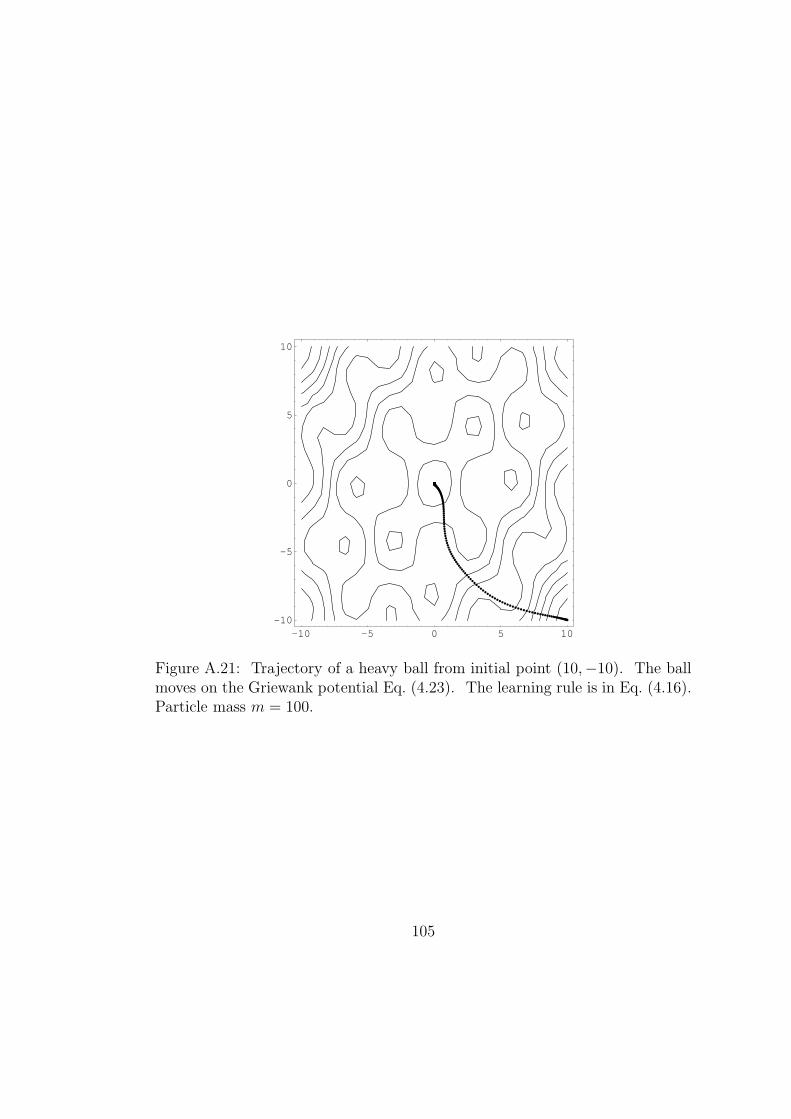
-10 -5 0 5 10-10

-5

0

5

10


105

Bibliography

[1] D. H. Ackley, G. E. Hinton, and T. J. Sejnowski. A learning algoreithm

for boltzmann machine. Cognitive science, 19:147, 1985.

[2] L. Adleman. Molecular computation of solutions to combinatorial prob-

lems. Science, 266:1021, 1994.

[3] S. Amari. Natural gradient works efficiently in learning. Neural Comput.,

10:251, 1998.

[4] Daniel J. Amit, Hanoch Gutfreund, and H. Sompolinsky. Storing infite

numbers of patterns in a spin-glass model of neural networks. Physical

Review Letters, 55:1530, 1985.

[5] H. Attouch, X. Goudou, and P. Redont. The heavy ball with friction

method, i. the continuous dynamical system: global exploration of the lo-

cal minima of a real-valued function by asymptotic analysis of a dissipative

dynamical system. Communications in Contemporary Mathematics, 2:1,

2000.

106

[6] Y. Benenson, B. Gil, U. Ben-Dor, R. Adar, and E. Shapiro. An autonomous

molecular computer for logical control of gene expression. Nature, 429:423,

2004.

[7] R. D. Blake, J. W. Bizzaro, J. D. Blake, G. R. Day, S. G. Delcourt,

J. Knowles, K. A. Marx, and J. SantaLucia Jr. Statistical mechanical

simulation of polymeric dna melting with meltsim. Bioinformatics, 15:370,

1999.

[8] R. S. Braich, N. Chelyapov, C. Johnson, P. W. K. Rothemund, and L. Adle-

man. Solution of a 20-variable 3-sat problem on a dna computer. Science,

296:499, 2002.

[9] A. Cabot. Inertia gradient-like dynamics system controlled by a stabilizing

term. Journal of Optimization Theory and Applications, 120:275, 2004.

[10] L. Caiani, L. Casetti, C. Clementi, and M. Pettini. Geometry of dynam-

ics, lyapunov exponents, and phase transition. Physical Review Letters,

79:4361, 1997.

[11] S-Y. Cho and T. W. S. Chow. Training multilayer neural networks using

fast global learning algorithm - least-squares and penalized optimization

methods. Neurocomputing, 25:115, 1999.

[12] P. Dayan, G. E. Hinton, R. M. Neal, and R. S. Zemel. The helmholtz

machine. Neural computation, 7:889, 1995.

107

[13] R. Deaton and M. Garzon. Thermodynamic constraints on dna-based com-

puting. In G. Paun, editor, Computing with Bio-Molecules: theory and

experiment, page 138, 1998.

[14] P. A. M. Dirac. General Theory of Relativity. Princeton university press,

1996.

[15] M. P. do Carmo. Differential geometry of curves and surfaces. Prentice–

Hall, 1976.

[16] S. Droste, T. Jansen, and I. Wegener. Dynamic parameter control in simple

evolutionary algorithms. Proc. of the Sixth Workshop on the Foundations

of Genetic Algorithms, page 275, 2001.

[17] A. Edelman, T. A. Arias, and S. T. Smith. The geometry of algorithms

with orthogonality constraints. Siam J. Matrix Anal. Appl., 20:303, 1998.

[18] A.E. Eiben and M. Schoenauer. Evolutionary computing. Information

Processing Letters, 82:1, 2002.

[19] R. Elghanian, J. J. Storhoff, R. C. Mucic, R. L. Letsinger, and C. A. Mirkin.

Selective colorimetric detection of polynucleotides based on the distance-

dependent optical properties of gold nanoparticles. Science, 277:1078, 1997.

[20] D. Faulhammer, A. R. Cukras, R. J. Lipton, and L. F. Landweber. Molecu-

lar computation: Rna solutions to chess problems. Proc. Natl. Acad. Sci.,

97:1385, 2000.

108

[21] R. P. Feynman. Feynman Lectures on Computation. Addison-Wesley, 1996.

[22] M. H. Garzon and R. J. Deaton. Codeword design and information encod-

ing in dna ensembles. Natural Computing, 3:253, 2004.

[23] J. A. Given, C.-O. Hwang, and M. Mascagni. First- and last-passege monte

carlo algorithms for the charge density distribution on a conducting surface.

Physical Review E, 66:056704, 2002.

[24] M. Guo, W. Chang, M. Ho, J. Lu, and J. Cao. Is optimal solution of

every np-complete or np-hard problem determined from its characteristic

for dna-based computing. BioSystems, 80:71, 2005.

[25] E. T. Jaynes. Information theory and statistical mechanics. Physical Re-

view, 106:620, 1957.

[26] J. SantaLucia Jr. and D. Hicks. The thermodynamics of dna structural

motifs. Annu. Rev. Biomol. Struct., 33:415, 2004.

[27] Joon Shik Kim, Jong Chan Kim, Jangmin O, and Byoung-Tak Zhang. A

global minimization algorithm based on a geodesic of a lagrangian formu-

lation of newtonian dynamics. Neural Processing Letters, 26:121, 2007.

[28] Joon Shik Kim, Ji-Woo Lee, Yung-Kyun Noh, Ji-Yoon Park, Dong-Yoon

Lee, Kyung-Ae Yang, Young Gyu Chai, Jong Chan Kim, and Byoung-

Tak Zhang. An evolutionary monte carlo algorithm for predicting dna

hybridization. BioSystems, 91:69, 2008.

109

[29] S. Kirkpatrick, C. D. Gelatt Jr., and M. P. Vecchi. Optimization by simu-

lated annealing. Science, 220:671, 1983.

[30] H. Klump and T. Ackermann. Experimental thermodynamics of the helix-

random coil transition. iv. influence of the base composition of dna on the

transition enthalpy. Biopolymers, 10:513, 1971.

[31] I. H. Lee, J. Y. Park, H. M. Jang, Y. G. Chai, and B. T. Zhang. Dna imple-

mentation of theorem proving with resolution refutation in propositional

logic. Lecture Notes in Computer Science, 2568:156, 2003.

[32] J. Y. Lee, S. Y. Shin, T. H. Park, and B. T. Zhang. Solving traveling sales-

man problem with dna molecules encoding numerical values. BioSystems,

78:39, 2004.

[33] J. B. Marion and S. T. Thornton. Classical dynamics of particles and

sysyems. Saunders colledge pub, Fort Worth, 1995.

[34] J. L. Martin. General relativity: A first course for physicists. Prentice-

Hall, 1995.

[35] N. Metropolis, A. W. Rosenbluth, M. N. Rosenbluth, and A. H. Teller.

Equation of state calculations by fast computing machines. J. Chem. Phys.,

21:1087, 1953.

[36] N. J. Nilsson. Atrificial intelligence: A new synthesis. Morgan Kaufmann

Publishers, Inc., San Francisco, CA, 1998.

110

[37] Y. Nishimori and S. Akaho. Learning algorithms utilizing quasi-geodesic

flows on the stiefel manifold. Neurocomputing, 67:106, 2005.

[38] N. Qian. On the momentum term in gradient descent learning algorithms.

Neural Networks, 12:145, 1999.

[39] F. Reif. Statistical physics. McGraw-Hill, 1965.

[40] D. E. Rumelhart, G. E. Hinton, and R. J. Williams. Learning representa-

tions by back–propagating errors. Nature, 323:533, 1986.

[41] J. J. Sakurai. Modern Quantum Mechanics. Addison-Wesley, 1994.

[42] G. Seelig, D. Soloveichik, D.Y. Zhang, and E. Winfree. Enzyme-free nucleic

acid logic circuits. Science, 314:1585, 2006.

[43] S. Y. Shin, D. Kim, I. H. Lee, and B. T. Zhang. Evolutionary sequence

generation for reliable dna computing. In D. B. Fogel, editor, Proceedings

of the Congress on Evolutionary Computation 2002, page 79. IEEE Press,

2002.

[44] S. Y. Shin, D. Kim, I. H. Lee, and B. T. Zhang. Multi-objective evolu-

tionary optimization of dna sequences for reliable dna computing. IEEE

Transactions on Evolutionary Computation, 2004.

[45] W. R. Smythe. Static and Dynamic Electricity. McGRAW-HILL, 1950.

[46] M. N. Stojanovic and D. Stefanovic. A deoxyribozyme-based molecular

automaton. Nature Biotechnology, 21:1069, 2003.

111

[47] K. R. Symon. Mechanics. Addison-Weasley, 1971.

[48] E. Winfree, F. Liu, L. A. Wenzler, and N. C. Seeman. Design and self-

assembly of two-dimensional dna crystals. Nature, 394:539, 1998.

[49] H. Yan, X. Zhang, Z. Shen, and N. C. Seeman. A robust dna mechanical

device controlled by hybridization topology. Nature, 415:62, 2002.

[50] K.-A. Yang, J.-H. Lee, I.-H. Lee, and B.-T. Zhang. A multiple microrna de-

tection system based on computational self-assembly of dna-gold nanopar-

ticles. Foundations of Nano Science 2007, page 67, 2007.

[51] B.-T. Zhang and D.-Y. Cho. System identification using evolutionary

markov chain monte carlo. J. Systems Architecture, 47:587, 2001.

[52] H. Zipper, H. Brunner, J. Bernhagen, and F. Vitzthum. Investigation

on dna intercalculation and surface binding by sybr green i, it’s structure

determination and methodological implications. Nucleic Acids Research,

32:e103, 2004.

112

�ï ��

Óüto��<Æõ� /BN�<Æ&h� ë�H]j[þt\� e��#Q"f þj&h��o��H ×�æ¹כ ��. ë�H]j[þt_� \V[þt

�Ð��H %i��<Æ\�"f_� ��Õª|½Ót�îß� �ª�d��, �ª�� o�<Æ\�"f_� �� ì�r�í ½ �l�, Õªo�

�¦ (��ÉÓ'� /BN�<Æ\�"f þj�èô�Ç_� q�6 x�¦ ��t��H W1àÔ0>ß¼ n��s� e��. s�M:

²DG�èþj�è°ú�כ¦�FG4�¤ ��¦��%i�þj�è°ú�כ¦ ½ ��H�¹ô�Çכs�þj&h��o\�e��#Q"f×�æכ

��½ ÅÒ]js��.

s� �7Hë�H\�"f��H Óüto��<Æ�¦ l�ìøÍÜ¼�Ð ��H í�H6£x ��H #Qu�a�A ~½ÓZO�s� >hµ1Ï

÷&%3��. �'pàÔ�Ðx�� Z�}�Ér �©�I�\�"f \��-t�� &h�#Qt��H �©�I��Ð r�Û¼%7��¦ ��

s�r�v�l�0AK�"f ¿º ��t� þj&h��o��|ÄÌs� [j0>&��. ì�r�� #Qu�a�A�Ér��s� )�|ÃÌ

u�\�¦ Z�}�Ér °úכ\�"f ±ú��Ér °úכÜ¼�Ð �]X� �#� �ÃÐÒ�o #3�0A\�¦ a%v)�çß��. ¢ô�Ç, í�H6£x

��H|½Ót�~½Ó~½Ó&ñd��ÉrÁº��î�r/BN_� |9�|¾Ó_��'a$íõ�í�H6£x ��H��¹1Ï�¦s�6 x � 9

s�M: �Ð:�x_� |½Ót�~½Ó ~½Ó&ñd��õ��H ²ú�o� r�çß�_� s�� ½Ós� e��.

Äºo��H p�o� >�S\��)a ¿º ��{�� DNA ��½+Ë�¦ #�$Á �y��_� éß�{9� DNA[þt�Ð

ÂÒ'�%3�l� 0A �#�z�o��BH(��ÉÓ'�ü<_�Û¼àÔÈÓÚÔ�©�\�"fì�r��#Qu�a�A�¦Ãº'��

%i��. s� ��½+Ëõ�&ñ�Ér &ño� 7£x"î ]j\�¦ ÉÒ��H ��\כ K�{©��)a��.

¢ô�Ç,��¹1Ï�¦~ÃÎ��HÁº��î�r/BN �4Sq�¦0Aô�Çí�H6£x ��H��¹1Ï>�Ãº��]jr�÷&

%3��. s� ��¹1Ï>�Ãº��H �ÐH$�ÚÔ2�¤õ� Õªo�~½Óß¼ �íJ$�[>�\�"f_� ��%i� þj&h��o �ÃÐÒ�o

\� s�6 x�)a��. s� í�H6£x ��H ��¹1Ï>�Ãº��H �¦�� %i��<Æ ��Õª|½Ót�îß�_� t��X<d��Ü¼

�Ð ÂÒ'� %3�#Q&��. Õª +þAI��H �íJ$�[>� �<ÊÃº_� �ÐÕª�<ÊÃº\�¦ r�çß�Ü¼�Ð p�ì�r ��¦

6£§Ãº\�¦ 2[ô�Ç °úכs��.

DNA_� ÂÒì�r&h�� J�� B�g�A�¦ :�xK�"f l�%3��¦ ��Ø�¦ ��H ��©� l�%3�z�+«>

113

s� d��o �<Æ_þvÜ¼�Ð ]jr�÷&#Qe��. ¢ô�Ç, �� "é¶óøÍ\�"f_�� ì�r�í�� í�H6£x �

��H |½Ót�~½Ó ~½Ó&ñd��Ü¼�ÐÂÒ'�%3�#Q|9�Ãº e��. s�ü< �'aº��)a X<s�'��s� �7Hë�H\�

]jr�÷&#Q e��. s� �7Hë�H\�"f ]jr�÷&��H ¿º ��t� ·ú��¦o�7£§[þt�Ér ��ª�ô�Ç ì�r��_�

q�5pwô�Ç �©�S!�[þt\�"f ]jl�÷&��H ��%i� þj&h��o ë�H]j[þt\� @/K�"f� &h�6 x|c ��sכ

�¦ l�@/�)a��.

ÅÒ¹#כQ : DNA ��½+Ë, r�ÓýtYUs�w�×¼ #Qu�a�A, ��¹1Ïs� e��H Áº��î�r /BN, í�H6£x&h�

��¹1Ï>�Ãº, ��%i� þj&h��o

Áþ� £U> : 98303-808

114

Acknowledgments

First, I appreciate the kind help from Prof. Jong Chan Kim in finishing this

thesis. He waited and encouraged me to complete my Ph.D program. Second,

I would like to thank Prof. Byoung-Tak Zhang for his kind teaching and guid-

ance in this academic field. From his guidance, I acquired the way of rational

thinking and writing skills. Third, I would like to thank Prof. Hyoung Chan

Bhang for his good teaching that lead me to achieve the prerequisite attitude of

an ideal scholar, especially, that of a Ph.D. This thesis paper was made possible

with his kind lessons. Fourth, I would like to thank Jangmin O, Yung-Kyun

Noh and Ji-Woo Lee. They helped me directly in producing this thesis. Fifth,

I would like to thank my senior and junior members at School of Physics and

Biointelligence laboratory. They sincerely helped me in dealing with the diffi-

culties during my Ph.D program. Sixth, I appreciate the devotion of my family,

especially my wife Shin, for supporting me in hard times and good times.

Finally I would like to thanks Jesus Christ who saved my life with his

blood on the cross two thousand years ago in Jerusalem.

115

Joon Shik Kim


February 2008

116

ÇÔ��+ ;³�

��$� �<ÆÂÒ M:ÂÒ'� $�_� t��§Ãº_��Ü¼�Ð Ãº�¦ �#� ÅÒ$4��¦ ~ÃÌ��õ�&ñ t��§Ãº

_��s� ÷&#QÅÒ�� 7áxðøÍ �§Ãº_��a� U�·�Ér y��\�¦ ×¼wn�m��. ��Òqt_��a�"f��H ]j

��~½ÓS!� � 9jËµ[þt#Q½+ÉM:\�&h�]X�ô�Ç ��õ�t��Ð#Q�9¹¡§�¦s�l��2�¤ �ü<ÅÒ

$4�_þvm��. ¢ô�Ç ~½Ó+þAðøÍ ��Òqt_��a�"f��H Dh�Ðs� t��§Ãº_��s� ÷&#Q ÅÒ39"f s�

�7Hë�Hs� òøÍÒqt ��2�¤ t��K� ÅÒ$4�_þvm��. Õªo��¦ (��ÉÓ'� /BN�<ÆÂÒ_� �©�#î�ÃÌ ��

Òqt_��a� U�·�Ér y��\�¦ ×¼wn�m��. ½�&h�Ü¼�Ð ��©� �>� ��êøÍ &h�[þt�¦ �2;]X� �

>� t�&h� �#� ÅÒ$4��¦ Õª t��Ð s� �7Hë�Hs� ¢-a$í÷&%3�_þvm��. Õªo��¦ Óüto��<ÆÂÒ

ü< BI��½z�_��ÊêC�#��Qì�r[þta�U�·�Éry��\�¦×¼wn�m��. �½Ó�©� ��>pwô�ÇÄº&ñ

Ü¼�Ð $�\�¦ ��9 �#� ÅÒ%3�_þvm��.

�7Hë�Hs� ��l��t� �©��}�ü< %òç�Hs� Õªo��¦ t�Äº��H µ1ß�¦ �FN&ñ&h��

_þvÜ¼�Ð ��½\� l�#� �#� ÅÒ%3�_þvm��. Õª ��s�\� °ú s� ��½ �%i�~�� ×�æ�©�@/ Óüt

o��<Æõ� s�ð�rd�� §Ãº_��õ� ��ÊêC�_��[þt Õªo��¦ "fÖ�¦@/ #î"é¶ Ùþ�_��<Æõ� ��Òqt_��[þt

õ� ��½"é¶[þta� d��d��ô�Ç y��\�¦ ×¼wn�m��. ��|½Ó_� �§�r\�"f ëß�èß� b��6£§_� +þA]j

[þta�� H y��\�¦ ×¼wn�m��. ��|ÃÌ~½Ó |9��_��[þtõ� ��|½Ó_� �§�r �2;½[þt�Ér �7Hë�H

�¦ æ¼��H õ�&ñ\�"f, jËµ[þt�¦ #Q�9Ö�¦ M:�� ×�æ�Ð l��\�¦ :�xK� 6 xl�\�¦ ÅÒ��H ²DI|�

ô�Ç !QhË>3lqs� ÷&#QÅÒ$4�_þvm��.

117

¢ô�Ç $�_� ��7á¤[þt \�>�� y��\�¦ ×¼wn�m��. $�_� |�� /BNÂÒ_� #�&ñ�¦ ¶nq

¶nqy� t�&��Ð 9 ��9\�¦ ��z�t� ·ú§��¤_þvm��. Õþ�e��y�� e��H ��©�_� �_þvÜ¼�Ð Õª

�ÉrK�\��Ð²ú� ��x_þvm��. ��t�}��Ü¼�Ð%�6£§ÂÒ'�t��FK��t�$�ü<�<Êa�K�ÅÒ��ÅÒ

_��a� ��H %òF�g�¦ [�twn�m��.

118

Stochastic and Deterministic Search Algorithms for Global ...jskim/PhD08s_KimJS.pdfStochastic and...

Documents

Transcript of Stochastic and Deterministic Search Algorithms for Global ...jskim/PhD08s_KimJS.pdfStochastic and...