Still Image Coding Standard – JPEGshi/courses/ECE789/ch7.pdf · Still Image Coding Standard –...
24
Chapter 7 Still Image Coding Standard – JPEG 7.1 Introduction • Since the mid-1980s, the ITU and ISO had been working together to develop a joint international standard for the compression of still images. • JPEG became an international standard in 1992. • Officially, JPEG [jpeg] is the ISO/IEC international standard 10918-1: digital compression and coding of continuous-tone still images, or the ITU-T Recommendation T.81. 1
Transcript of Still Image Coding Standard – JPEGshi/courses/ECE789/ch7.pdf · Still Image Coding Standard –...
Chapter 7
Still Image Coding Standard – JPEG
7.1 Introduction
• Since the mid-1980s, the ITU and ISO had been working together to develop a joint international standard for the compression of still images.
• JPEG became an international standard in
1992. • Officially, JPEG [jpeg] is the ISO/IEC
international standard 10918-1: digital compression and coding of continuous-tone still images, or the ITU-T Recommendation T.81.
1
♦ JPEG includes two classes of encoding and decoding processes:
§ Lossy process
DCT-based sufficient for many applications
§ Lossless process Prediction-based
♦ JPEG includes four modes of operation
§ Sequential DCT-based mode § Progressive DCT-based mode § Lossless mode § Hierarchical mode.
v Sequential DCT-based mode § an image first partitioned into blocks of
8x8 pixels § then the blocks processed from left to
right, top to bottom. 2
§ 8x8 2-D forward DCT is applied to each block § 8x8 DCT coefficients then quantized § quantized DCT coefficients entropy
encoded and output v Progressive DCT-based mode § Similar to sequential DCT-based mode § Quantized DCT coefficients, however,
first stored in buffer. § DCT coefficients in buffer then encoded
by a multiple scanning process § In each scan, quantized DCT coefficients
partially encoded either by spectral selection or successive approximation.
ü In spectral selection, quantized DCT
coefficients divided into multiple spectral bands according to the zig-zag order.
3
In each scan, a specified band is encoded.
ü In successive approximation, a
specified number of most significant bits of quantized coefficients first encoded. In subsequent scans, less significant bits are encoded.
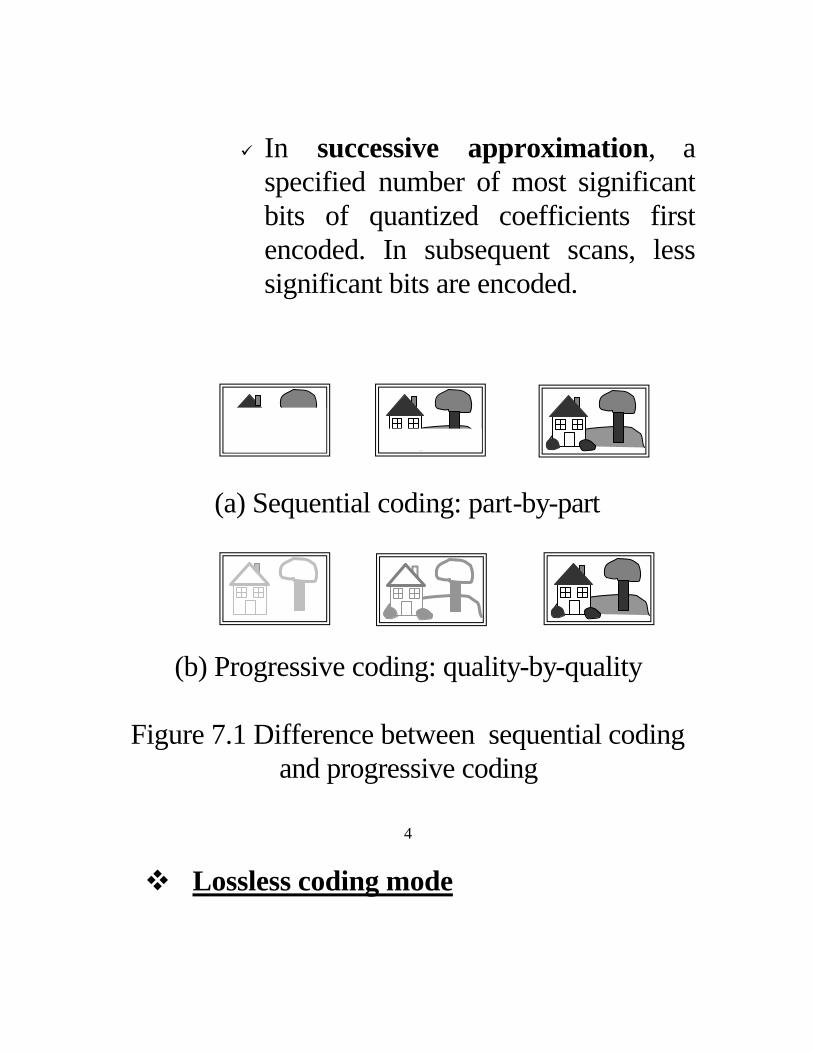
(a) Sequential coding: part-by-part
(b) Progressive coding: quality-by-quality
Figure 7.1 Difference between sequential coding and progressive coding
4
v Lossless coding mode
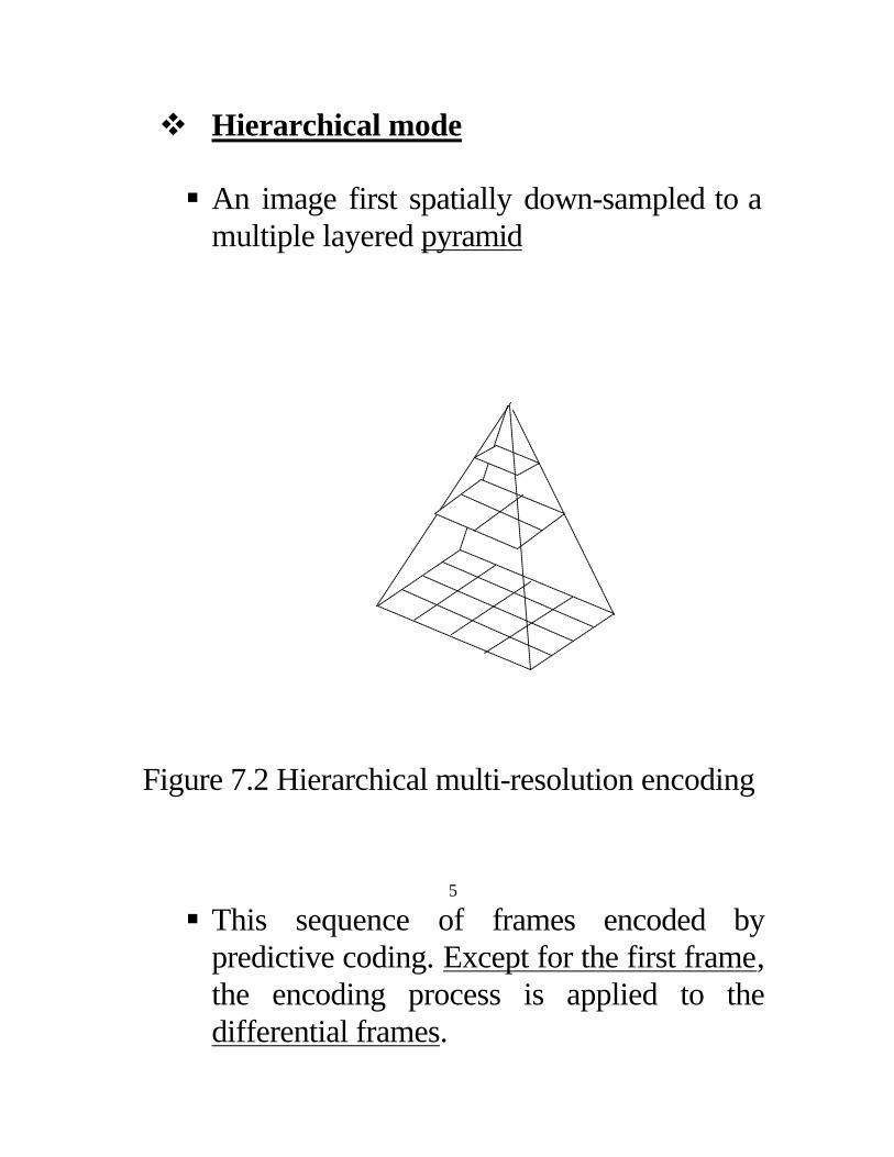
v Hierarchical mode § An image first spatially down-sampled to a
multiple layered pyramid
Figure 7.2 Hierarchical multi-resolution encoding 5
§ This sequence of frames encoded by predictive coding. Except for the first frame, the encoding process is applied to the differential frames.
§ Hierarchical coding mode provides a
progressive presentation similar to progressive DCT-based mode but is useful in the applications, which have multi-resolution requirements.
§ Hierarchical mode also provides the
capability of progressive coding to a final lossless stage.
7.2 Sequential DCT-based encoding algorithm
• Baseline algorithm (heart) of JPEG coding standard.
6
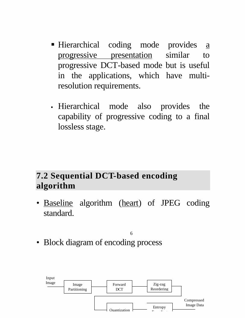
• Block diagram of encoding process
Input Image Image
Partitioning Forward
DCT Zig-zag
Reordering
Quantization Entropy
Encoding
Compressed Image Data
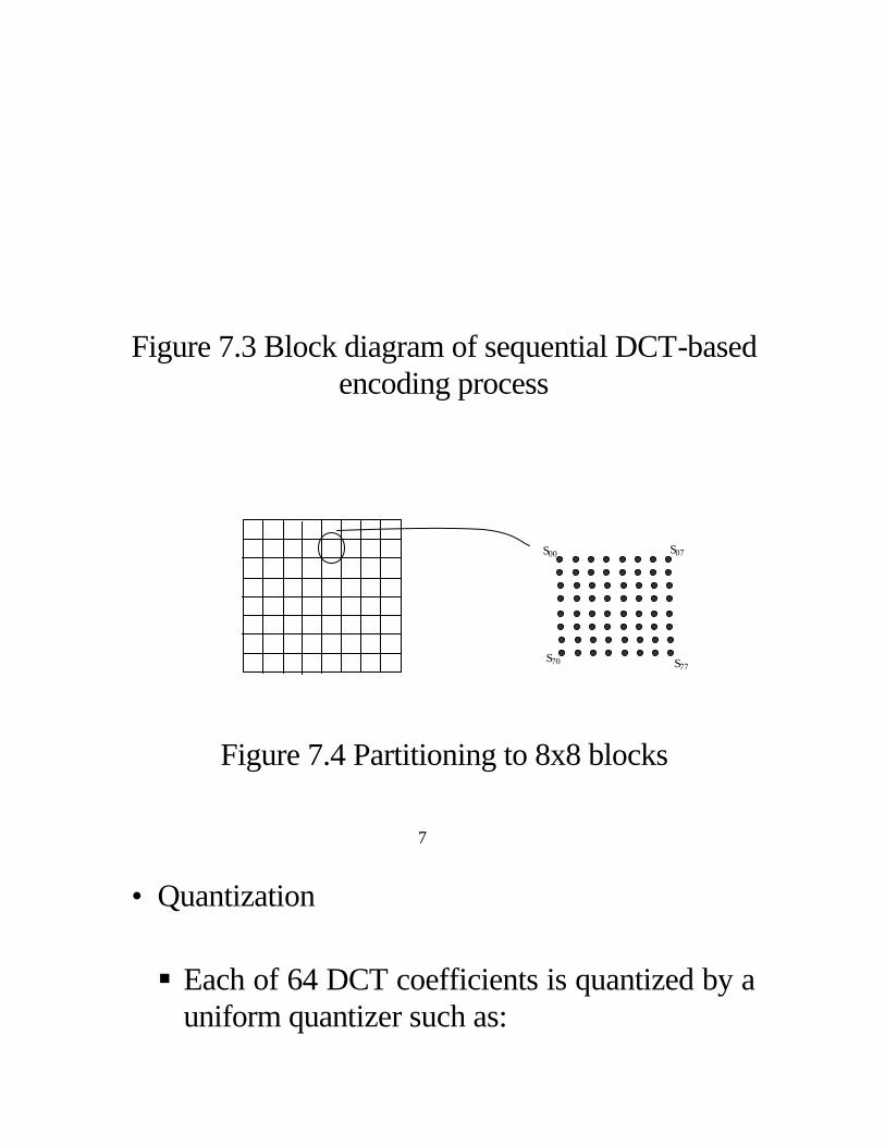
Figure 7.3 Block diagram of sequential DCT-based encoding process
Figure 7.4 Partitioning to 8x8 blocks
7
• Quantization
§ Each of 64 DCT coefficients is quantized by a uniform quantizer such as:
S07 S00
S70 S77
Squv : quantized value of the DCT coefficient, Suv,
Quv : quantization step obtained from the quantization table.
§ Four quantization tables, which may be used by encoder § No default quantization tables specified in the
specification. 8
§ Some typical quantization tables are as follows:
S roundSQquv
uv
uv
= ( )
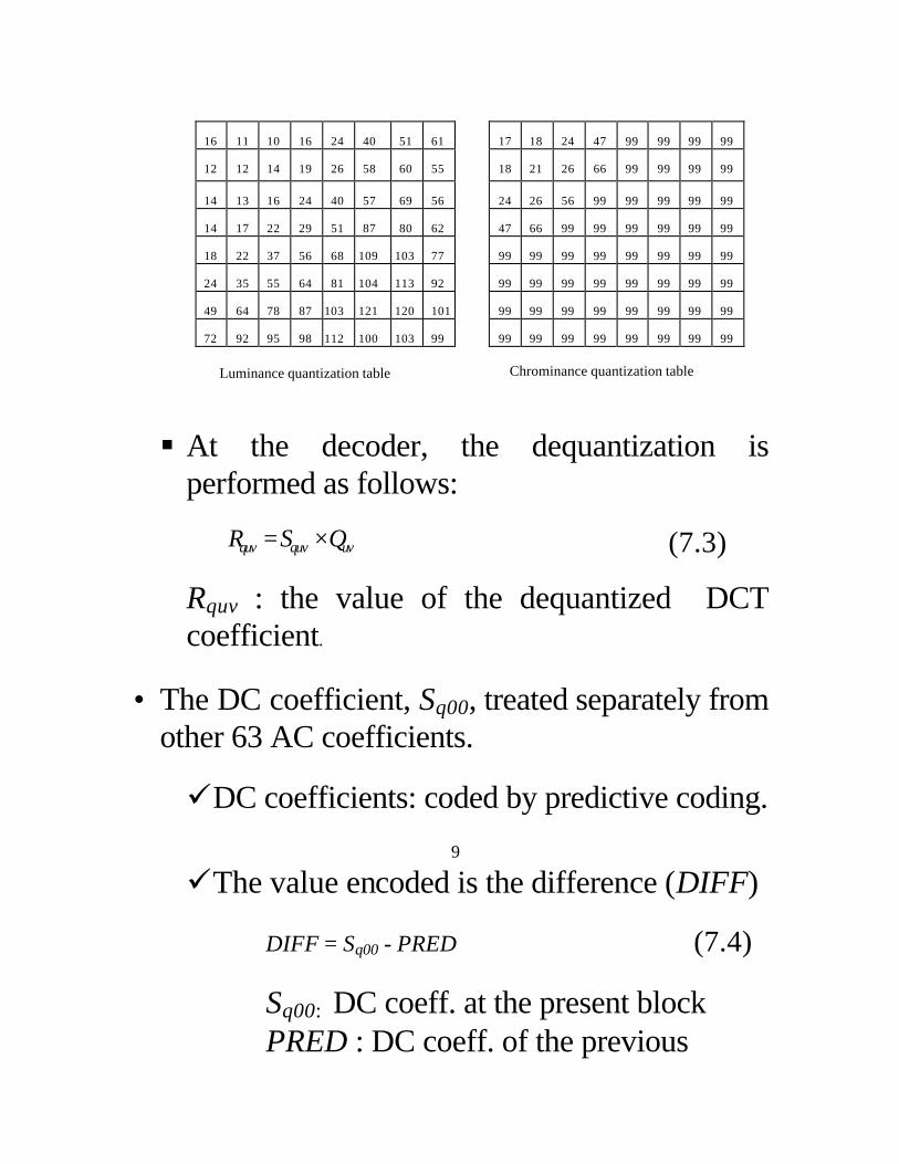
16 11 10 16 24 40 51 61 17 18 24 47 99 99 99 99
12 12 14 19 26 58 60 55 18 21 26 66 99 99 99 99
14 13 16 24 40 57 69 56 24 26 56 99 99 99 99 99
14 17 22 29 51 87 80 62 47 66 99 99 99 99 99 99
18 22 37 56 68 109 103 77 99 99 99 99 99 99 99 99
24 35 55 64 81 104 113 92 99 99 99 99 99 99 99 99
49 64 78 87 103 121 120 101 99 99 99 99 99 99 99 99
72 92 95 98 112 100 103 99
99 99 99 99 99 99 99 99
§ At the decoder, the dequantization is performed as follows:
Rquv : the value of the dequantized DCT coefficient.
• The DC coefficient, Sq00, treated separately from other 63 AC coefficients.
ü DC coefficients: coded by predictive coding.
9 ü The value encoded is the difference (DIFF)
DIFF = Sq00 - PRED (7.4)
Sq00: DC coeff. at the present block PRED : DC coeff. of the previous
Luminance quantization table Chrominance quantization table
R S Qquv quv uv= × (7.3)
block
ü Diff is coded by Huffman coding.
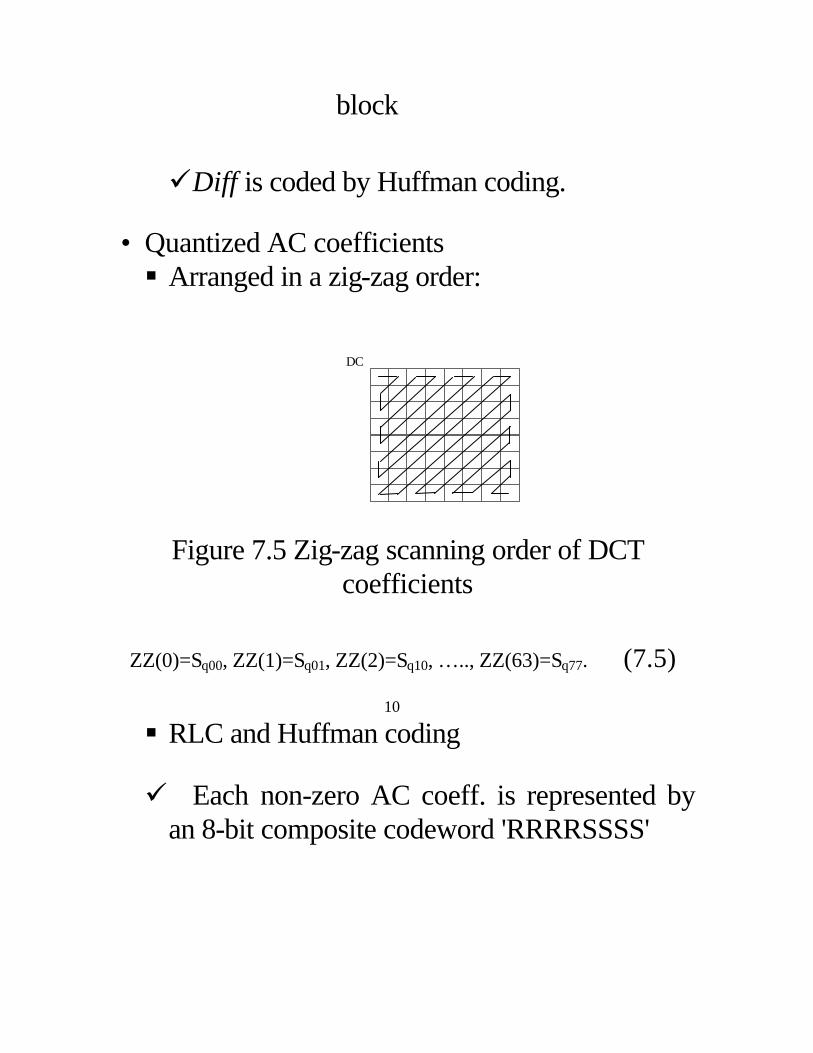
• Quantized AC coefficients § Arranged in a zig-zag order:
Figure 7.5 Zig-zag scanning order of DCT coefficients
ZZ(0)=Sq00, ZZ(1)=Sq01, ZZ(2)=Sq10, … .., ZZ(63)=Sq77. (7.5) 10
§ RLC and Huffman coding ü Each non-zero AC coeff. is represented by
an 8-bit composite codeword 'RRRRSSSS'
DC
ü 4 most significant bits 'RRRR': the run-length of zeros from the previous nonzero coeff.
ü 4 least significant bits 'SSSS': the value of
the non-zero coefficient which ends the zero-run (10 categories).
ü Category k : ( 12,2 1 −− kk ) or (- 12 +k ,- 12 −k ) ü 'RRRRSSSS'=11110000: a run-length of 16
zero coefficients ü Run-length exceeding 16 needs multiple
symbols. ü 'RRRRSSSS' = '00000000': the end-of-block
(EOB) [remaining coefficients in the block are zero].
11
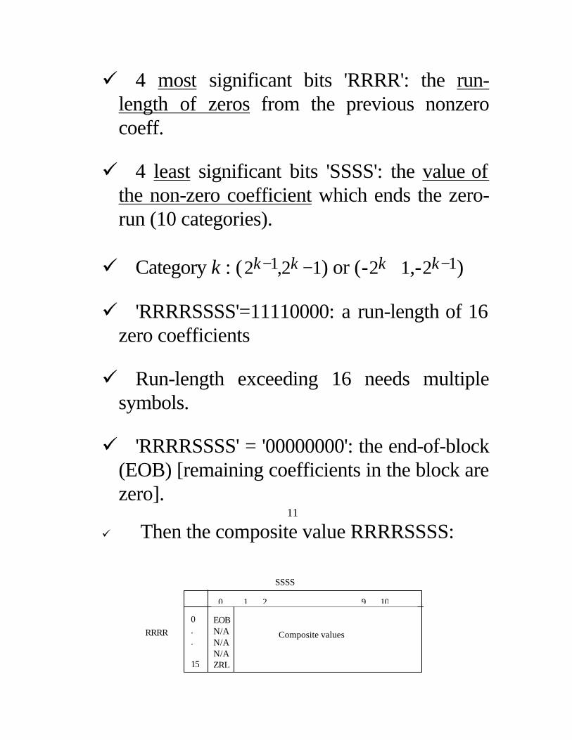
ü Then the composite value RRRRSSSS:
SSSS
0 . . 15
0 1 2 9 10
EOB N/A N/A N/A ZRL
Composite values RRRR
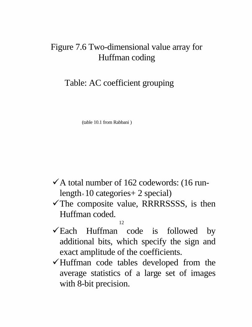
Figure 7.6 Two-dimensional value array for Huffman coding
Table: AC coefficient grouping
(table 10.1 from Rabbani )
ü A total number of 162 codewords: (16 run-length×10 categories+ 2 special) ü The composite value, RRRRSSSS, is then
Huffman coded. 12
ü Each Huffman code is followed by additional bits, which specify the sign and exact amplitude of the coefficients. ü Huffman code tables developed from the
average statistics of a large set of images with 8-bit precision.
ü An adaptive arithmetic coding procedure can be also used for entropy coding.
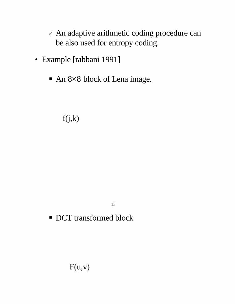
• Example [rabbani 1991] § An 88× block of Lena image.
f(j,k)
13
§ DCT transformed block
F(u,v)
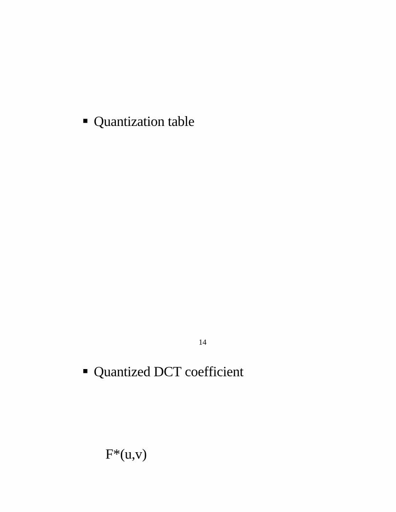
§ Quantization table 14
§ Quantized DCT coefficient
F*(u,v)
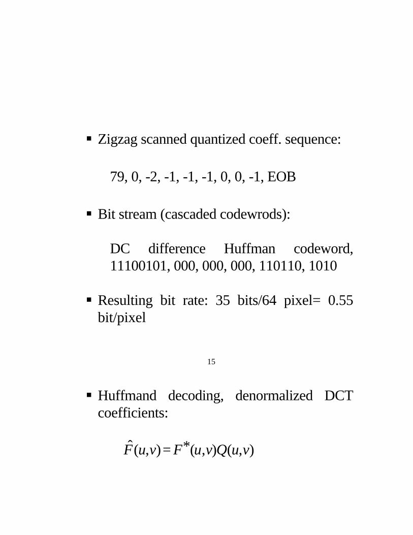
§ Zigzag scanned quantized coeff. sequence:
79, 0, -2, -1, -1, -1, 0, 0, -1, EOB
§ Bit stream (cascaded codewrods):
DC difference Huffman codeword, 11100101, 000, 000, 000, 110110, 1010
§ Resulting bit rate: 35 bits/64 pixel= 0.55 bit/pixel
15
§ Huffmand decoding, denormalized DCT coefficients:
),(),(*),(̂ vuQvuFvuF =
§ IDCT
f^(j,k)
16
§ Reconstruction error
e(j,k)
§ RMSE
RMSE= 2.26 17
7.3 Progressive DCT-based encoding algorithm
• Blcokwise 2-D 8x8 DCT
• Quantizized DCT-coefficients: encoded with
multiple scans. § At each scan, a portion of the DCT coefficient
data is encoded. § This partial encoded data can be reconstructed
to obtain a full image size with lower picture quality.
§ The coded data of each additional scan will
enhance the reconstructed image quality until the full quality has been achieved at the completion of all scans.
18
• Two methods: § spectral selection § successive approximation
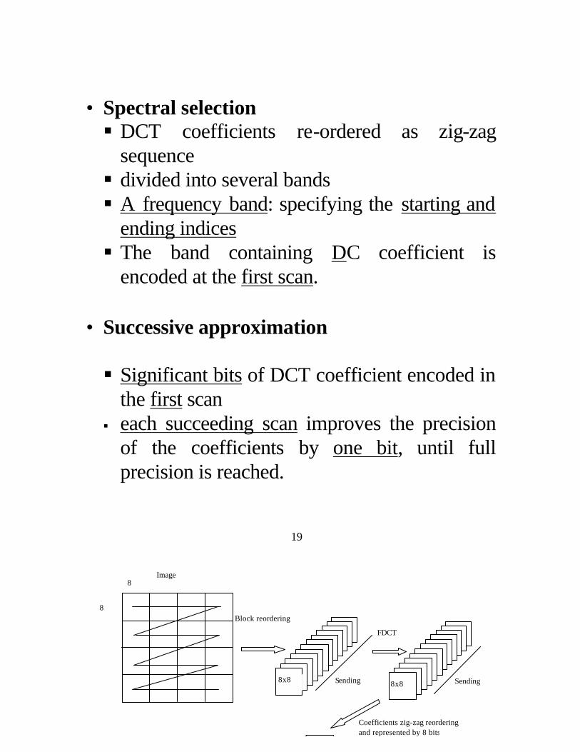
• Spectral selection § DCT coefficients re-ordered as zig-zag
sequence § divided into several bands § A frequency band: specifying the starting and
ending indices § The band containing DC coefficient is
encoded at the first scan.
• Successive approximation § Significant bits of DCT coefficient encoded in
the first scan § each succeeding scan improves the precision
of the coefficients by one bit, until full precision is reached.
19
Image
Block reordering
FDCT
8
8
8x8 8x8 Sending Sending
Coefficients zig-zag reordering and represented by 8 bits
Figure 7.6 Progressive coding with spectral selection and successive approximation
7.4 Lossless coding mode
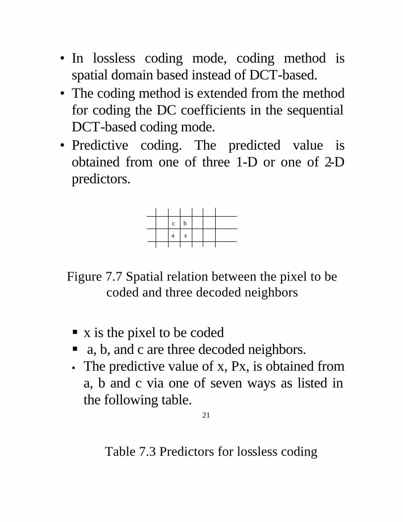
• In lossless coding mode, coding method is spatial domain based instead of DCT-based.
• The coding method is extended from the method for coding the DC coefficients in the sequential DCT-based coding mode.
• Predictive coding. The predicted value is obtained from one of three 1-D or one of 2-D predictors.
Figure 7.7 Spatial relation between the pixel to be coded and three decoded neighbors
§ x is the pixel to be coded § a, b, and c are three decoded neighbors. § The predictive value of x, Px, is obtained from
a, b and c via one of seven ways as listed in the following table.
21
Table 7.3 Predictors for lossless coding
c b
a x
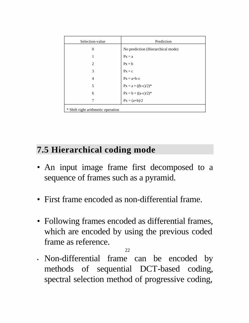
Selection-value Prediction
0
1
2
3
4
5
6
7
No prediction (Hierarchical mode)
Px = a
Px = b
Px = c
Px = a+b-c
Px = a + ((b-c)/2)*
Px = b + ((a-c)/2)*
Px = (a+b)/2
* Shift right arithmetic operation
7.5 Hierarchical coding mode
• An input image frame first decomposed to a sequence of frames such as a pyramid.
• First frame encoded as non-differential frame. • Following frames encoded as differential frames,
which are encoded by using the previous coded frame as reference.
22
• Non-differential frame can be encoded by methods of sequential DCT-based coding, spectral selection method of progressive coding,
or lossless coding with either Huffman code or arithmetic code.
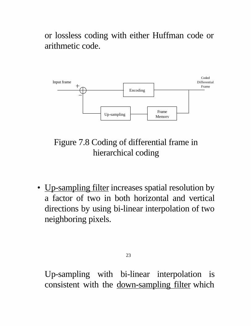
Figure 7.8 Coding of differential frame in hierarchical coding
• Up-sampling filter increases spatial resolution by a factor of two in both horizontal and vertical directions by using bi-linear interpolation of two neighboring pixels.
23
Up-sampling with bi-linear interpolation is consistent with the down-sampling filter which
Up-sampling Frame
Memory
Encoding
Input frame Coded
Differential Frame
is used for the generation of down-sampled frames.
References [jpeg] Digital compression and coding of continuous-tone still images - Requirements and Guidelines, ISO-/IEC International Standard 10918-1, CCITT T.81, September, 1992. [pennebaker 1993] W. B. Pennebaker and J. L. Mitchell, JPEG Still Image Data Compression Standard, New York: Van Nostrand Reinhold, 1993. [rabbani 1991] M. Rabbani and P. W. Jones, Digital Image Compression Techniques, Bellingham, WA: SPIE Optical Engineering Press, 1991.
24