Sticky Wages and Prices: Aggregate Expenditure and...
71
5 Topic Sticky Wages and Prices: Aggregate Expenditure and the Multiplier
Transcript of Sticky Wages and Prices: Aggregate Expenditure and...
5TopicSticky Wages and Prices:
Aggregate Expenditure and the
Multiplier
Questioning the Classical Position and
the Self-Regulating Economy
John Maynard Keynes, an English economist, changed how
many economists viewed the economy.
Keynes’s major work, The General Theory of employment,
Interest and Money, was published in 1936.
Just prior to its publication, the Great Depression had plagued
many countries of the world.
Unemployment was sky-high in many countries, and many
economies had been contracting.

Questioning the Classical Position and
the Self-Regulating Economy
Where was Say’s law, with its promise that there would be no
general gluts?
When was the self-regulating economy going to heal itself of
its depression illness?
Where was full employment?
And, given the depressed state of the economy, could anyone
any longer believe that laissez-faire was the right policy?
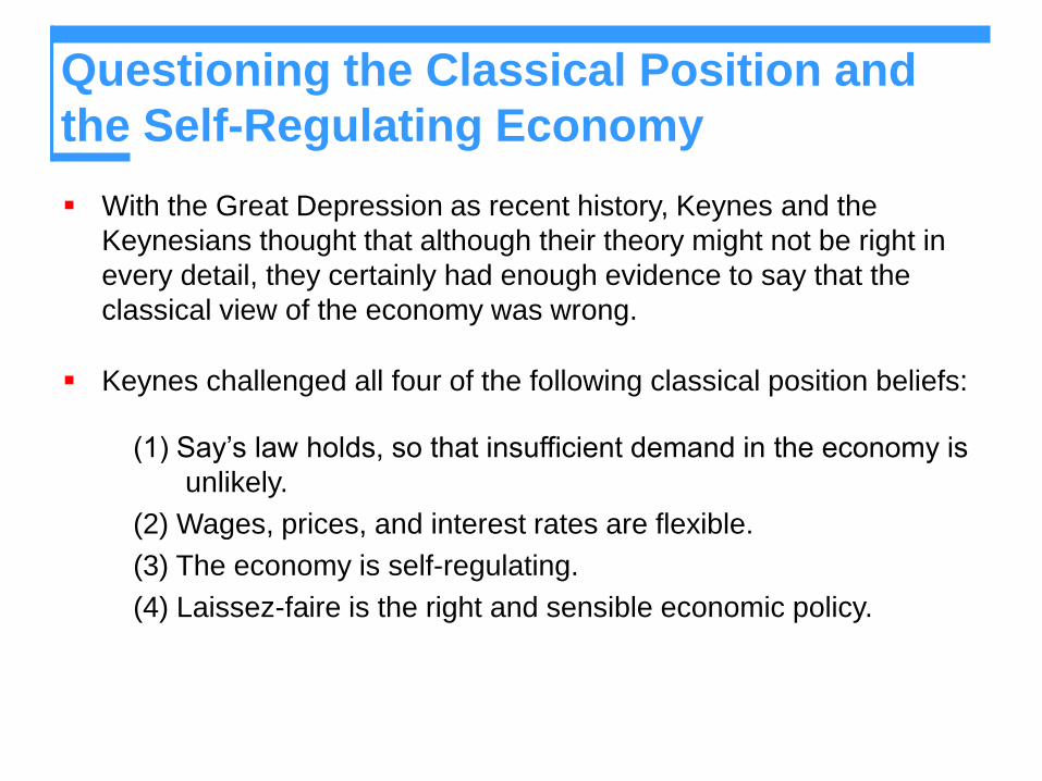
With the Great Depression as recent history, Keynes and the
Keynesians thought that although their theory might not be right in
every detail, they certainly had enough evidence to say that the
classical view of the economy was wrong.
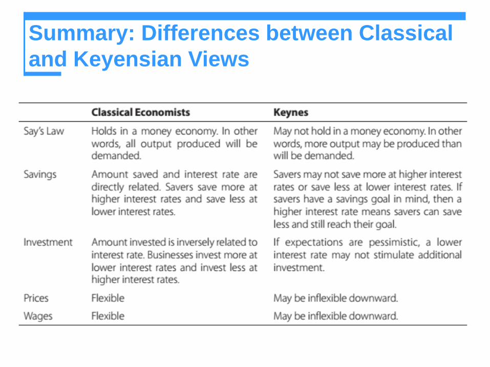
Keynes challenged all four of the following classical position beliefs:
(1) Say’s law holds, so that insufficient demand in the economy is
unlikely.
(2) Wages, prices, and interest rates are flexible.
(3) The economy is self-regulating.
(4) Laissez-faire is the right and sensible economic policy.
Questioning the Classical Position and
the Self-Regulating Economy
Keynes’s Criticism of Say’s Law in a
Money Economy
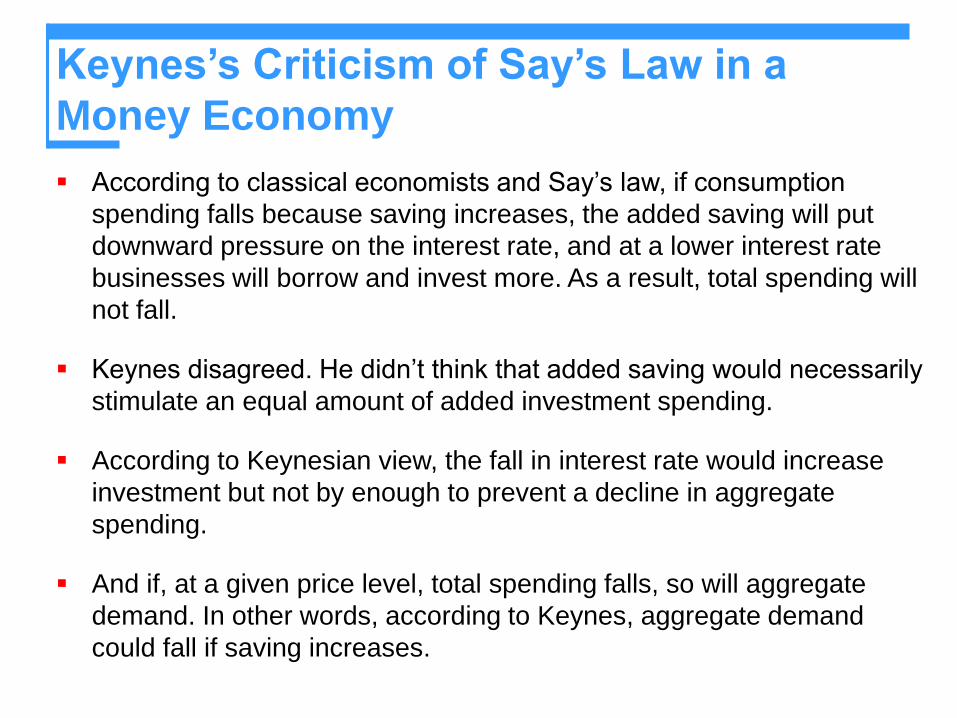
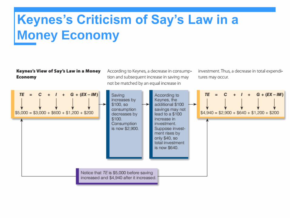
According to classical economists and Say’s law, if consumption
spending falls because saving increases, the added saving will put
downward pressure on the interest rate, and at a lower interest rate
businesses will borrow and invest more. As a result, total spending will
not fall.
Keynes disagreed. He didn’t think that added saving would necessarily
stimulate an equal amount of added investment spending.
According to Keynesian view, the fall in interest rate would increase
investment but not by enough to prevent a decline in aggregate
spending.
And if, at a given price level, total spending falls, so will aggregate
demand. In other words, according to Keynes, aggregate demand
could fall if saving increases.
Keynes’s Criticism of Say’s Law in a
Money Economy
Keynes’s Criticism of Say’s Law in a
Money Economy
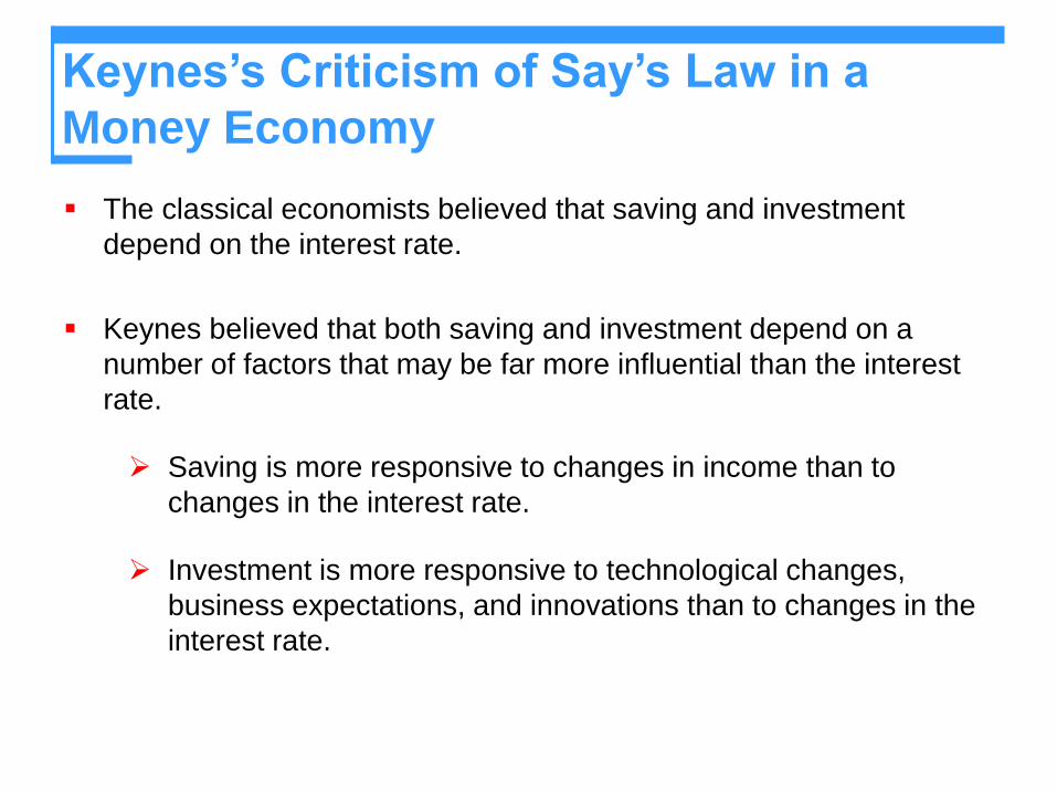
The classical economists believed that saving and investment
depend on the interest rate.
Keynes believed that both saving and investment depend on a
number of factors that may be far more influential than the interest
rate.
Saving is more responsive to changes in income than to
changes in the interest rate.
Investment is more responsive to technological changes,
business expectations, and innovations than to changes in the
interest rate.
Keynes’s Criticism of Say’s Law in a
Money Economy
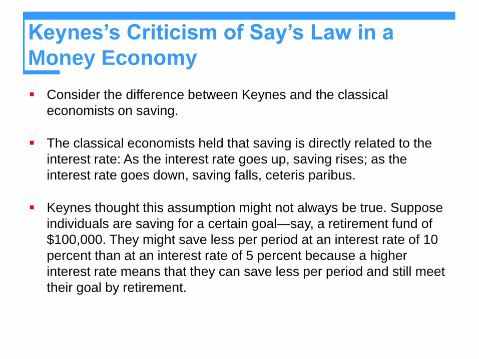
Consider the difference between Keynes and the classical
economists on saving.
The classical economists held that saving is directly related to the
interest rate: As the interest rate goes up, saving rises; as the
interest rate goes down, saving falls, ceteris paribus.
Keynes thought this assumption might not always be true. Suppose
individuals are saving for a certain goal—say, a retirement fund of
$100,000. They might save less per period at an interest rate of 10
percent than at an interest rate of 5 percent because a higher
interest rate means that they can save less per period and still meet
their goal by retirement.
Keynes’s Criticism of Say’s Law in a
Money Economy
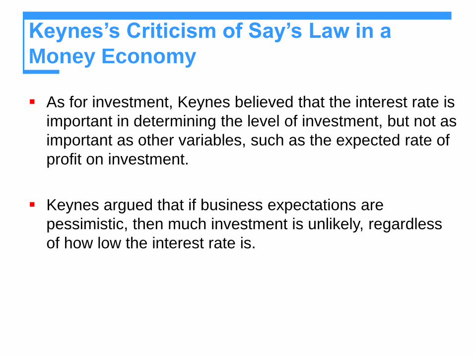
As for investment, Keynes believed that the interest rate is
important in determining the level of investment, but not as
important as other variables, such as the expected rate of
profit on investment.
Keynes argued that if business expectations are
pessimistic, then much investment is unlikely, regardless
of how low the interest rate is.
Keynes on Wage Rates
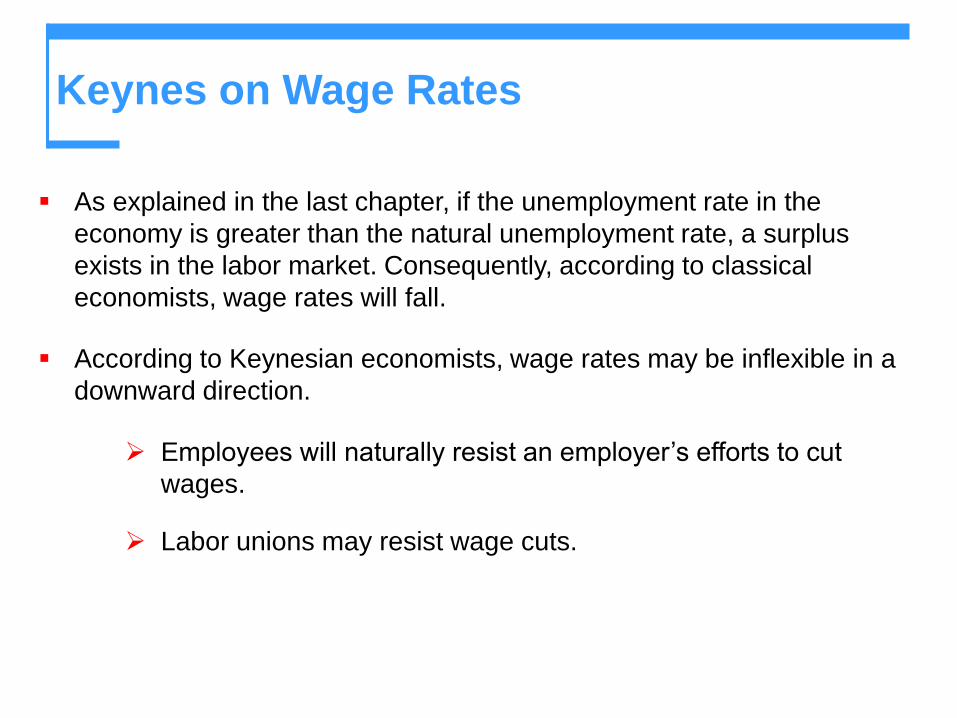
As explained in the last chapter, if the unemployment rate in the
economy is greater than the natural unemployment rate, a surplus
exists in the labor market. Consequently, according to classical
economists, wage rates will fall.
According to Keynesian economists, wage rates may be inflexible in a
downward direction.
Employees will naturally resist an employer’s efforts to cut
wages.
Labor unions may resist wage cuts.
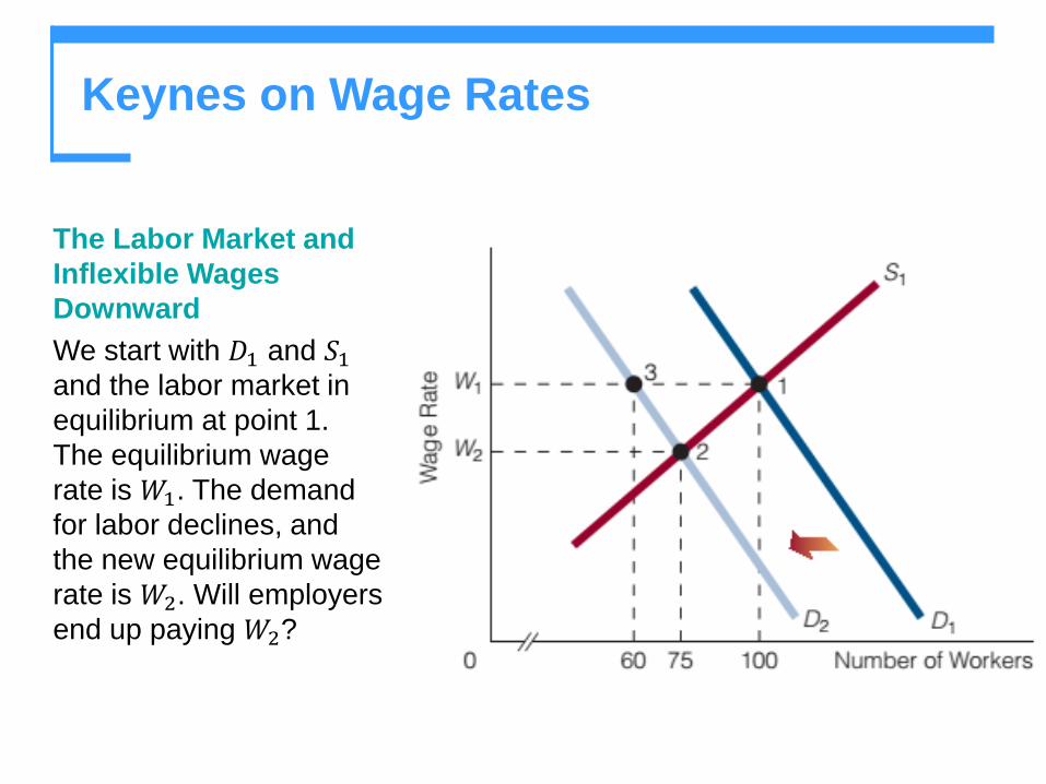
The Labor Market and
Inflexible Wages
Downward
We start with 𝐷1 and 𝑆1and the labor market in
equilibrium at point 1.
The equilibrium wage
rate is 𝑊1. The demand
for labor declines, and
the new equilibrium wage
rate is 𝑊2. Will employers
end up paying 𝑊2?
Keynes on Wage Rates
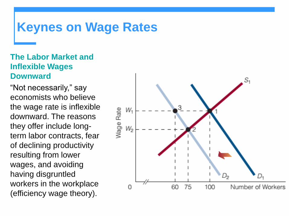
The Labor Market and
Inflexible Wages
Downward
“Not necessarily,” say
economists who believe
the wage rate is inflexible
downward. The reasons
they offer include long-
term labor contracts, fear
of declining productivity
resulting from lower
wages, and avoiding
having disgruntled
workers in the workplace
(efficiency wage theory).
Keynes on Wage Rates
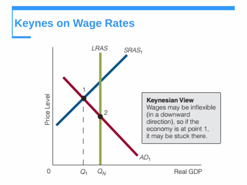
Keynes on Wage Rates
If Keynes is correct and wage rates will not fall, is the
economy then unable to get itself out of a recessionary gap?
The unequivocal answer is yes.
If employee and labor union resistance prevents wage rates
from falling, then the SRAS curve will not shift to the right. If it
does not shift to the right, the price level won’t come down. If
the price level does not come down, buyers will not purchase
more goods and services and move the economy out of a
recessionary gap.
Keynes believed that the economy is inherently unstable and
that it may not automatically cure itself of a recessionary gap.
It may not be self-regulating.
Keynes on Wage Rates
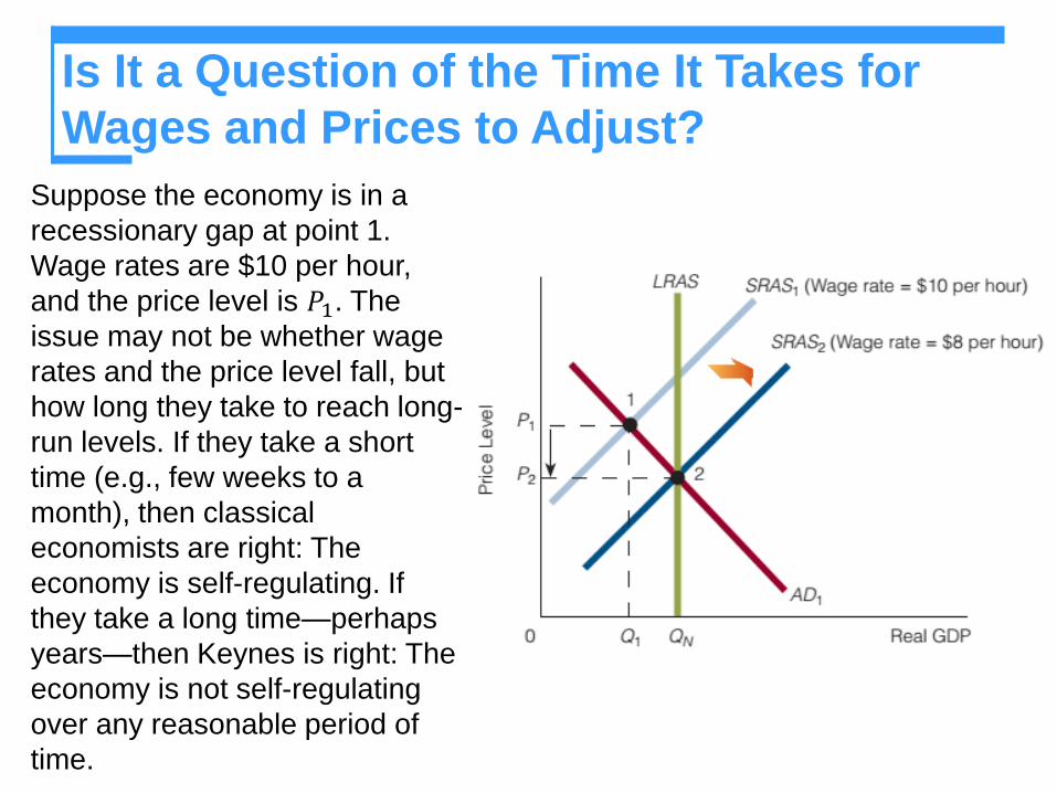
Is It a Question of the Time It Takes for
Wages and Prices to Adjust?
Suppose the economy is in a
recessionary gap at point 1.
Wage rates are $10 per hour,
and the price level is 𝑃1. The
issue may not be whether wage
rates and the price level fall, but
how long they take to reach long-
run levels. If they take a short
time (e.g., few weeks to a
month), then classical
economists are right: The
economy is self-regulating. If
they take a long time—perhaps
years—then Keynes is right: The
economy is not self-regulating
over any reasonable period of
time.
Keynes on Prices
Again, recall what classical economists believe occurs when a
recessionary gap exists: Wage rates fall, the SRAS curve shifts to the
right, and the price level begins to decrease—stop right there! The
phrase “the price level begins to decrease” tells us that classical
economists believe that prices in the economy are flexible: They move
up and down in response to market forces.
Keynes said that the internal structure of an economy is not always
competitive enough to allow prices to fall. Anticompetitive or
monopolistic elements in the economy sometimes prevent price from
falling.
Summary: Differences between Classical
and Keyensian Views
The Keynesian Model
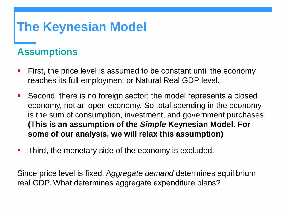
Assumptions
First, the price level is assumed to be constant until the economy
reaches its full employment or Natural Real GDP level.
Second, there is no foreign sector: the model represents a closed
economy, not an open economy. So total spending in the economy
is the sum of consumption, investment, and government purchases.
(This is an assumption of the Simple Keynesian Model. For
some of our analysis, we will relax this assumption)
Third, the monetary side of the economy is excluded.
Since price level is fixed, Aggregate demand determines equilibrium
real GDP. What determines aggregate expenditure plans?
Fixed Prices and Expenditure Plans
Expenditure Plans
The components of aggregate expenditure sum to real
GDP.
That is,
Y = C + I + G + X – M.
Two of the components of aggregate expenditure,
consumption and imports, are influenced by real GDP.
So there is a two-way link between aggregate expenditure
and real GDP.
Fixed Prices and Expenditure Plans
Two-Way Link Between Aggregate Expenditure and Real
GDP
Other things remaining the same,
An increase in real GDP increases aggregate expenditure.
An increase in aggregate expenditure increases real GDP.
Fixed Prices and Expenditure Plans
Consumption and Saving Plans
Consumption expenditure is influenced by many factors
but the most direct one is disposable income.
Disposable income is aggregate income or real GDP, Y,
minus net taxes, T.
Call disposable income YD.
The equation for disposable income is
YD = Y – T
Fixed Prices and Expenditure Plans
Disposable income, YD, is either spent on consumption
goods and services, C, or saved, S.
That is,
YD = C + S.
The relationship between consumption expenditure and
disposable income, other things remaining the same, is
the consumption function.
The relationship between saving and disposable income,
other things remaining the same, is the saving function.
Figure in the next slide illustrates the consumption function
and the saving function.
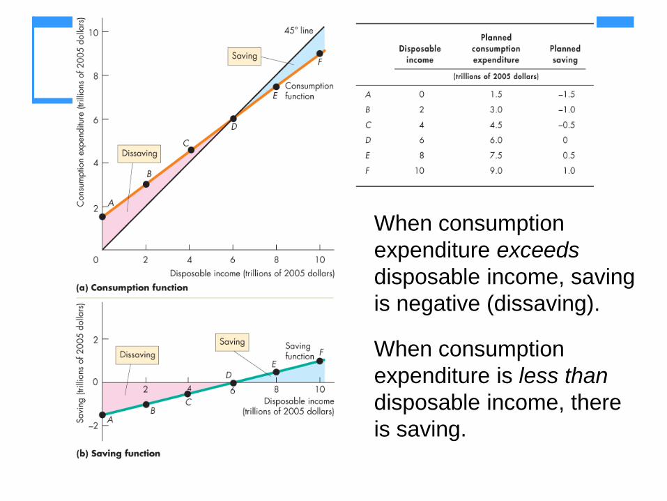
When consumption
expenditure exceeds
disposable income, saving
is negative (dissaving).
When consumption
expenditure is less than
disposable income, there
is saving.
Fixed Prices and Expenditure Plans
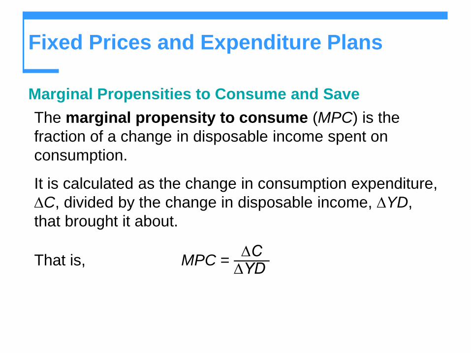
Marginal Propensities to Consume and Save
The marginal propensity to consume (MPC) is the
fraction of a change in disposable income spent on
consumption.
It is calculated as the change in consumption expenditure,
C, divided by the change in disposable income, YD,
that brought it about.
That is, MPC = C
YD
Fixed Prices and Expenditure Plans
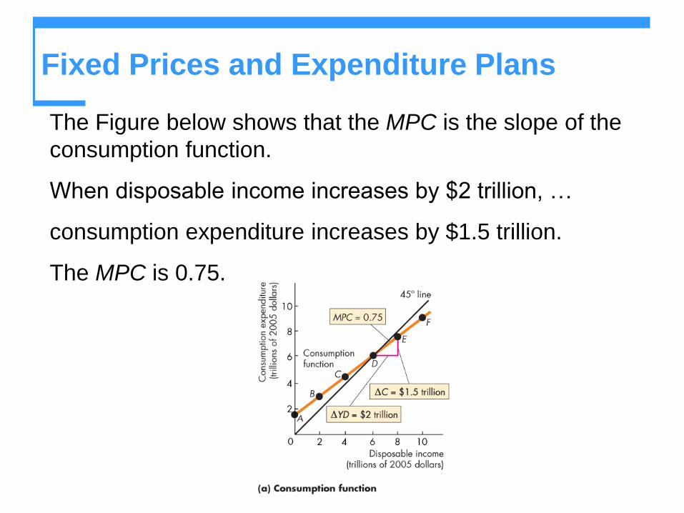
The Figure below shows that the MPC is the slope of the
consumption function.
When disposable income increases by $2 trillion, …
consumption expenditure increases by $1.5 trillion.
The MPC is 0.75.
Fixed Prices and Expenditure Plans
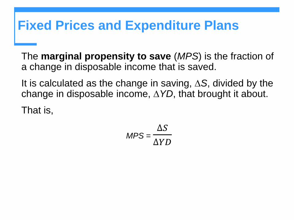
The marginal propensity to save (MPS) is the fraction of a change in disposable income that is saved.
It is calculated as the change in saving, S, divided by the change in disposable income, YD, that brought it about.
That is,
MPS = ∆𝑆
∆𝑌𝐷
Fixed Prices and Expenditure Plans
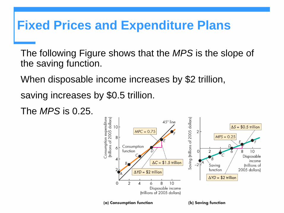
The following Figure shows that the MPS is the slope of the saving function.
When disposable income increases by $2 trillion,
saving increases by $0.5 trillion.
The MPS is 0.25.
Fixed Prices and Expenditure Plans
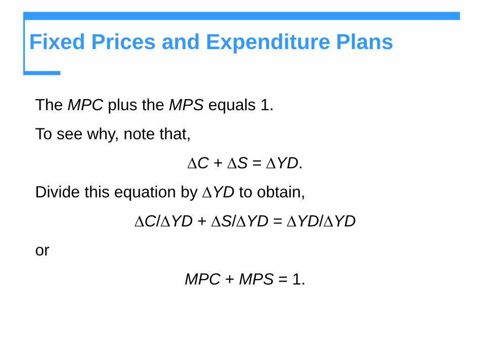
The MPC plus the MPS equals 1.
To see why, note that,
C + S = YD.
Divide this equation by YD to obtain,
C/YD + S/YD = YD/YD
or
MPC + MPS = 1.
Fixed Prices and Expenditure Plans
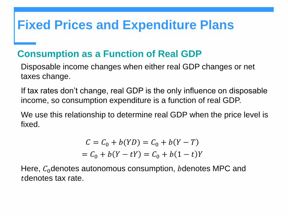
Consumption as a Function of Real GDP
Disposable income changes when either real GDP changes or net
taxes change.
If tax rates don’t change, real GDP is the only influence on disposable
income, so consumption expenditure is a function of real GDP.
We use this relationship to determine real GDP when the price level is
fixed.
𝐶 = 𝐶0 + 𝑏(𝑌𝐷) = 𝐶0 + 𝑏 𝑌 − 𝑇
= 𝐶0 + 𝑏 𝑌 − 𝑡𝑌 = 𝐶0 + 𝑏 1 − 𝑡 𝑌
Here, 𝐶0denotes autonomous consumption, 𝑏denotes MPC and
𝑡denotes tax rate.
Fixed Prices and Expenditure Plans
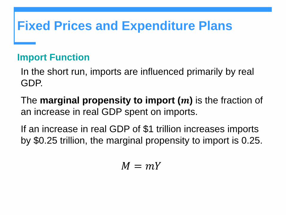
Import Function
In the short run, imports are influenced primarily by real
GDP.
The marginal propensity to import (𝒎) is the fraction of
an increase in real GDP spent on imports.
If an increase in real GDP of $1 trillion increases imports
by $0.25 trillion, the marginal propensity to import is 0.25.
𝑀 = 𝑚𝑌
Real GDP with a Fixed Price Level
Consumption expenditure minus imports, which varies with
real GDP, is induced expenditure.
The sum of investment, government expenditure, and
exports, which does not vary with GDP, is autonomous
expenditure.
Consumption as explained before also has an autonomous
component.
Real GDP with a Fixed Price Level
Aggregate Planned Expenditure
The relationship between aggregate planned expenditure
and real GDP can be described by an aggregate
expenditure schedule, which lists the level of aggregate
expenditure planned at each level of real GDP.
The relationship can also be described by an aggregate
expenditure curve, which is a graph of the aggregate
expenditure schedule.
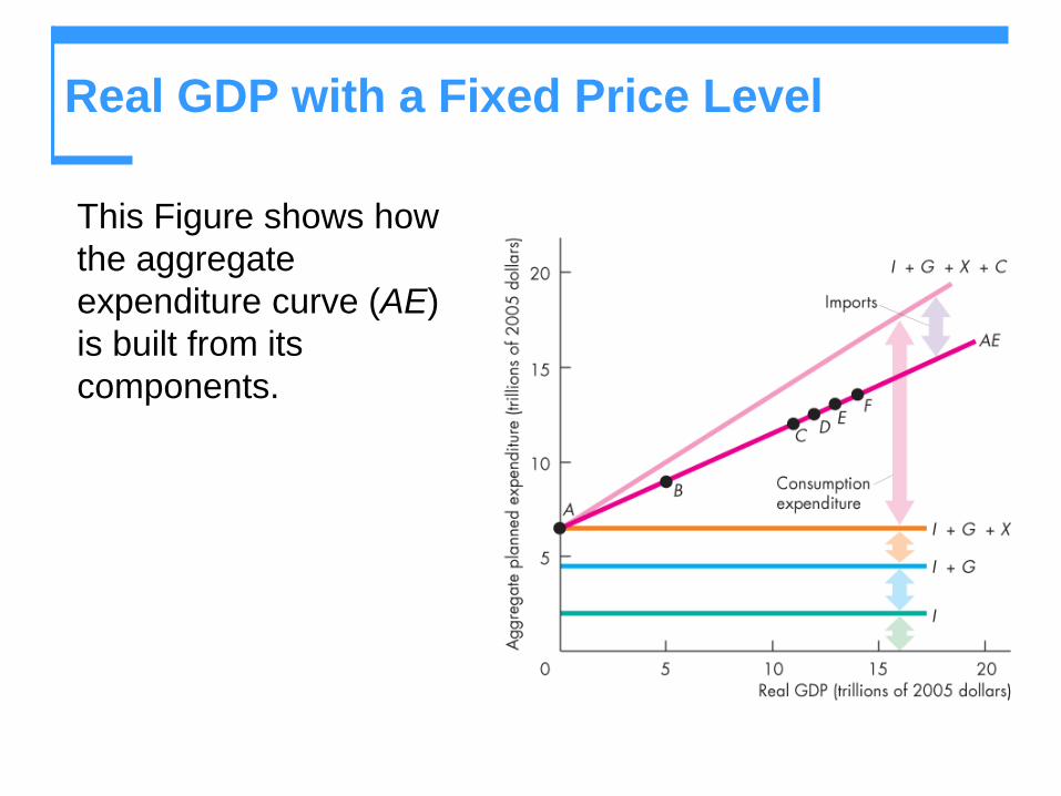
Real GDP with a Fixed Price Level
This Figure shows how
the aggregate
expenditure curve (AE)
is built from its
components.
Real GDP with a Fixed Price Level
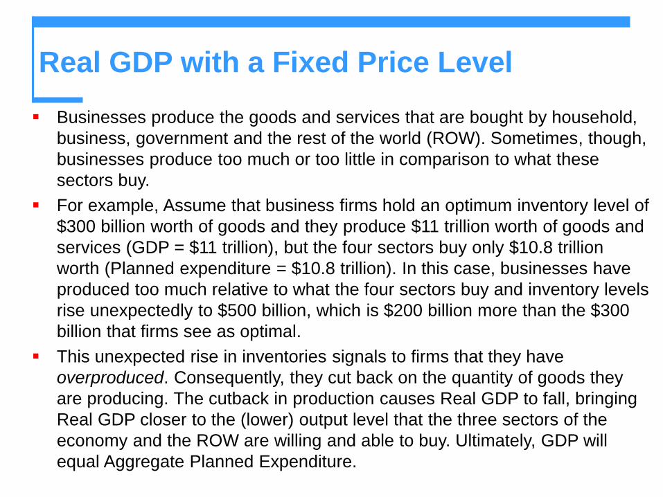
Businesses produce the goods and services that are bought by household,
business, government and the rest of the world (ROW). Sometimes, though,
businesses produce too much or too little in comparison to what these
sectors buy.
For example, Assume that business firms hold an optimum inventory level of
$300 billion worth of goods and they produce $11 trillion worth of goods and
services (GDP = $11 trillion), but the four sectors buy only $10.8 trillion
worth (Planned expenditure = $10.8 trillion). In this case, businesses have
produced too much relative to what the four sectors buy and inventory levels
rise unexpectedly to $500 billion, which is $200 billion more than the $300
billion that firms see as optimal.
This unexpected rise in inventories signals to firms that they have
overproduced. Consequently, they cut back on the quantity of goods they
are producing. The cutback in production causes Real GDP to fall, bringing
Real GDP closer to the (lower) output level that the three sectors of the
economy and the ROW are willing and able to buy. Ultimately, GDP will
equal Aggregate Planned Expenditure.
Real GDP with a Fixed Price Level
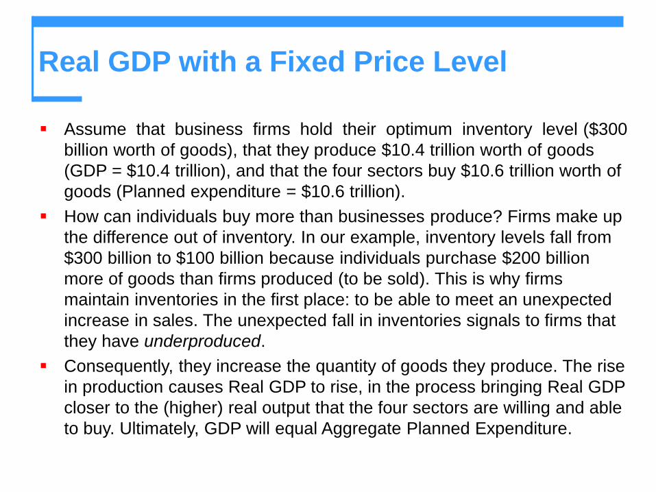
Assume that business firms hold their optimum inventory level ($300
billion worth of goods), that they produce $10.4 trillion worth of goods
(GDP = $10.4 trillion), and that the four sectors buy $10.6 trillion worth of
goods (Planned expenditure = $10.6 trillion).
How can individuals buy more than businesses produce? Firms make up
the difference out of inventory. In our example, inventory levels fall from
$300 billion to $100 billion because individuals purchase $200 billion
more of goods than firms produced (to be sold). This is why firms
maintain inventories in the first place: to be able to meet an unexpected
increase in sales. The unexpected fall in inventories signals to firms that
they have underproduced.
Consequently, they increase the quantity of goods they produce. The rise
in production causes Real GDP to rise, in the process bringing Real GDP
closer to the (higher) real output that the four sectors are willing and able
to buy. Ultimately, GDP will equal Aggregate Planned Expenditure.
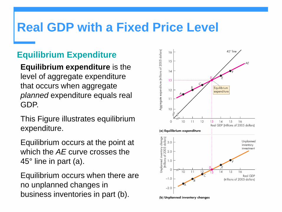
Real GDP with a Fixed Price Level
Equilibrium Expenditure
Equilibrium expenditure is the
level of aggregate expenditure
that occurs when aggregate
planned expenditure equals real
GDP.
This Figure illustrates equilibrium
expenditure.
Equilibrium occurs at the point at
which the AE curve crosses the
45° line in part (a).
Equilibrium occurs when there are
no unplanned changes in
business inventories in part (b).
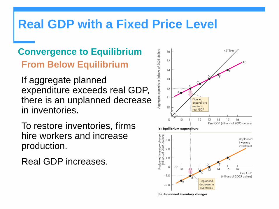
Real GDP with a Fixed Price Level
Convergence to Equilibrium
From Below Equilibrium
If aggregate planned expenditure exceeds real GDP, there is an unplanned decrease in inventories.
To restore inventories, firms hire workers and increase production.
Real GDP increases.
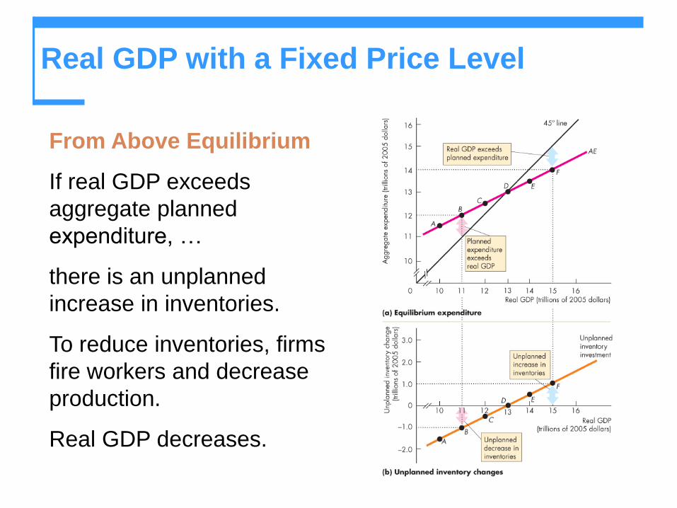
Real GDP with a Fixed Price Level
From Above Equilibrium
If real GDP exceeds
aggregate planned
expenditure, …
there is an unplanned
increase in inventories.
To reduce inventories, firms
fire workers and decrease
production.
Real GDP decreases.
Real GDP with a Fixed Price Level
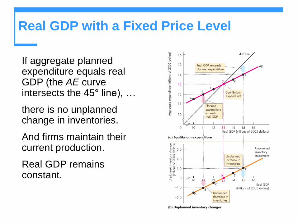
If aggregate planned expenditure equals real GDP (the AE curve intersects the 45° line), …
there is no unplanned change in inventories.
And firms maintain their current production.
Real GDP remains constant.
The Multiplier
When autonomous expenditure changes, so does
equilibrium expenditure and real GDP.
But the change in equilibrium expenditure is larger than
the change in autonomous expenditure.
The multiplier is the amount by which a change in
autonomous expenditure is magnified or multiplied to
determine the change in equilibrium expenditure and real
GDP.
The Multiplier
The Basic Idea of the Multiplier
An increase in investment (or any other component of
autonomous expenditure) increases aggregate
expenditure and real GDP.
The increase in real GDP leads to an increase in induced
expenditure.
The increase in induced expenditure leads to a further
increase in aggregate expenditure and real GDP.
So real GDP increases by more than the initial increase in
autonomous expenditure.
The Multiplier
Why Is the Multiplier Greater than 1?
The multiplier is greater than 1 because an increase in
autonomous expenditure induces further increases in
aggregate expenditure.
The Size of the Multiplier
The size of the multiplier is the change in equilibrium
expenditure divided by the change in autonomous
expenditure.
The Multiplier
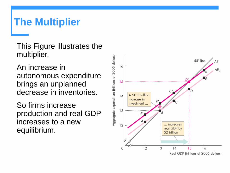
This Figure illustrates the multiplier.
An increase in autonomous expenditure brings an unplanned decrease in inventories.
So firms increase production and real GDP increases to a new equilibrium.
The Multiplier
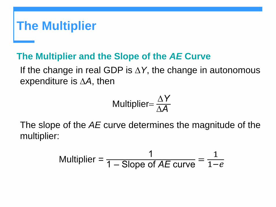
The Multiplier and the Slope of the AE Curve
If the change in real GDP is Y, the change in autonomous
expenditure is A, then
Multiplier= YA
The slope of the AE curve determines the magnitude of the
multiplier:
Multiplier = 1
1 – Slope of AE curve=
11−𝑒
The Multiplier
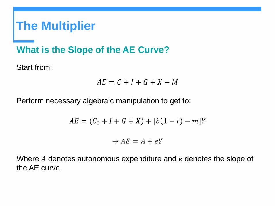
What is the Slope of the AE Curve?
Start from:
𝐴𝐸 = 𝐶 + 𝐼 + 𝐺 + 𝑋 −𝑀
Perform necessary algebraic manipulation to get to:
𝐴𝐸 = 𝐶0 + 𝐼 + 𝐺 + 𝑋 + 𝑏 1 − 𝑡 − 𝑚 𝑌
→ 𝐴𝐸 = 𝐴 + 𝑒𝑌
Where 𝐴 denotes autonomous expenditure and 𝑒 denotes the slope of
the AE curve.
The Multiplier
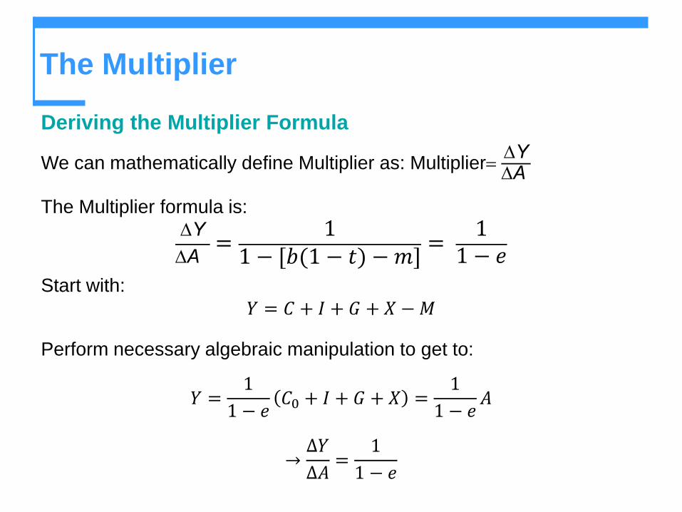
Deriving the Multiplier Formula
We can mathematically define Multiplier as: Multiplier= YA
The Multiplier formula is:
Y
A=
11 − 𝑏 1 − 𝑡 − 𝑚
=1
1 − 𝑒
Start with:
𝑌 = 𝐶 + 𝐼 + 𝐺 + 𝑋 −𝑀
Perform necessary algebraic manipulation to get to:
𝑌 =1
1 − 𝑒𝐶0 + 𝐼 + 𝐺 + 𝑋 =
1
1 − 𝑒𝐴
→∆𝑌
∆𝐴=
1
1 − 𝑒
The Multiplier
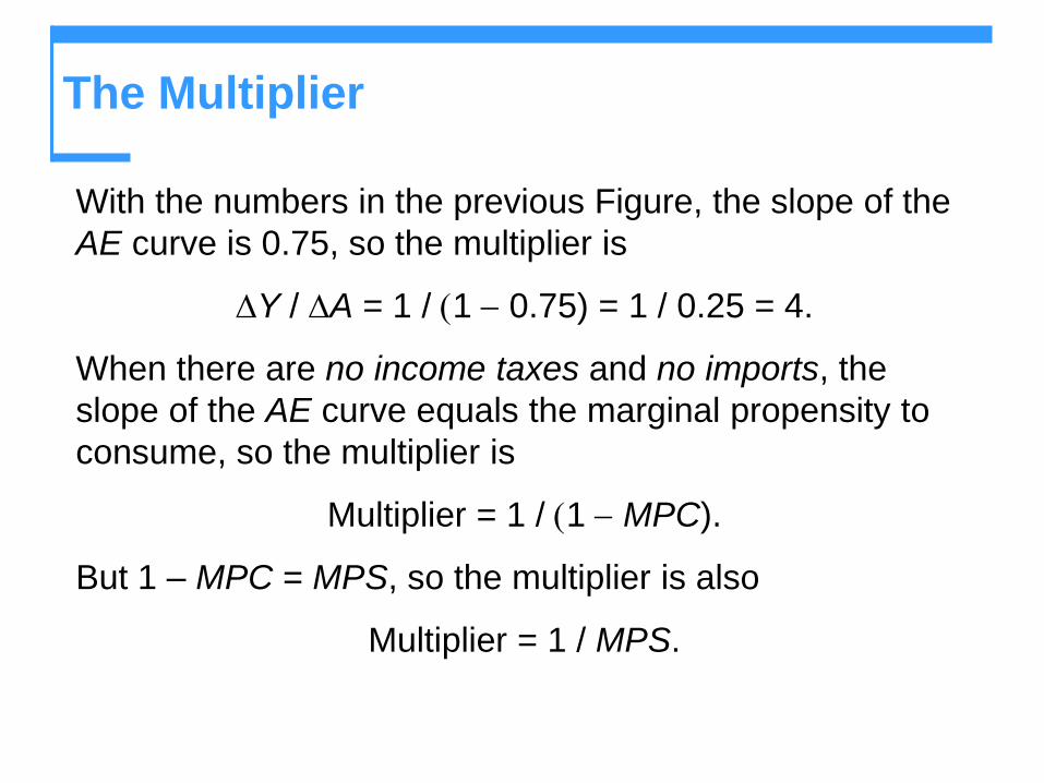
With the numbers in the previous Figure, the slope of the
AE curve is 0.75, so the multiplier is
Y / A = 1 / (1 - 0.75) = 1 / 0.25 = 4.
When there are no income taxes and no imports, the
slope of the AE curve equals the marginal propensity to
consume, so the multiplier is
Multiplier = 1 / (1 - MPC).
But 1 – MPC = MPS, so the multiplier is also
Multiplier = 1 / MPS.
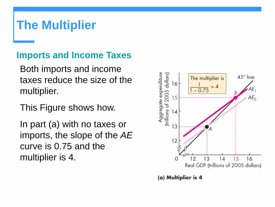
The Multiplier
Imports and Income Taxes
Both imports and income
taxes reduce the size of the
multiplier.
This Figure shows how.
In part (a) with no taxes or
imports, the slope of the AE
curve is 0.75 and the
multiplier is 4.
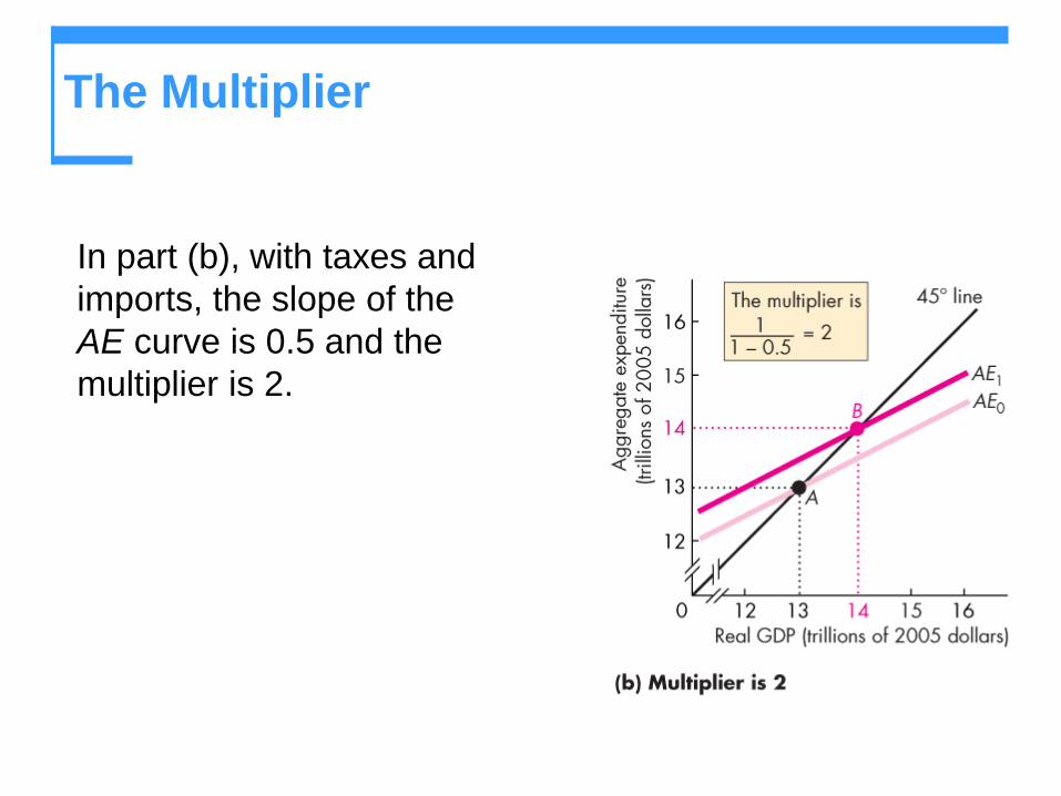
The Multiplier
In part (b), with taxes and
imports, the slope of the
AE curve is 0.5 and the
multiplier is 2.
The Multiplier
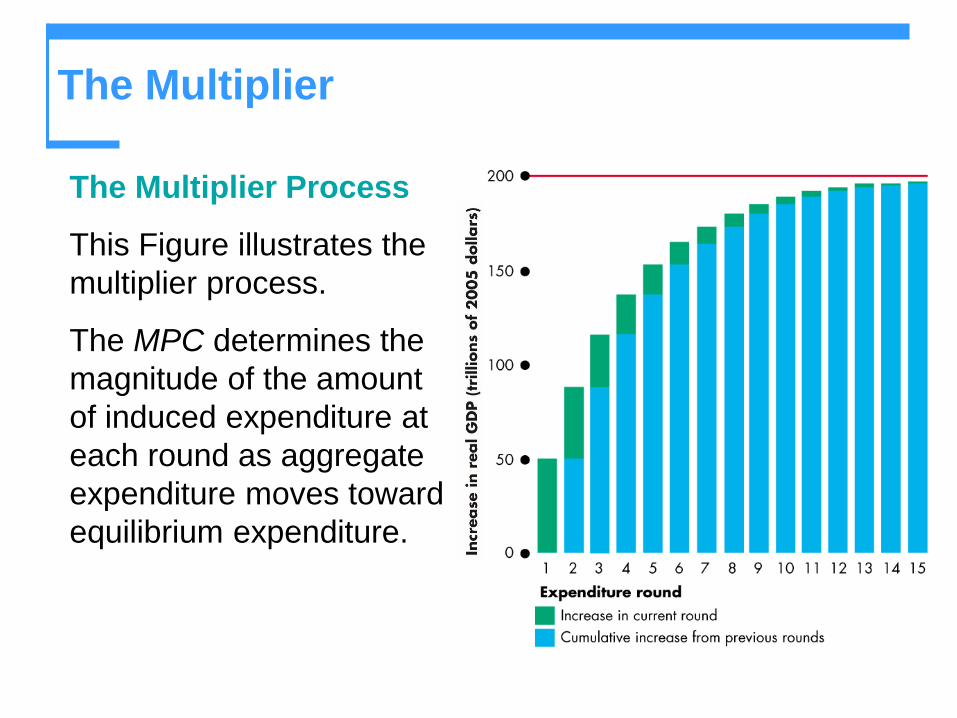
The Multiplier Process
This Figure illustrates the
multiplier process.
The MPC determines the
magnitude of the amount
of induced expenditure at
each round as aggregate
expenditure moves toward
equilibrium expenditure.
The Multiplier and Reality
So, in simple terms, a change in autonomous spending leads
to a greater change in total spending.
Also, in the Keynesian model, the change in total spending is
equal to the change in Real GDP (assuming that the economy
is operating below Natural Real GDP).
The reason is that, in the model, prices are assumed to be
constant until Natural GDP is reached; so any change in
nominal total spending is equal to the change in real total
spending.
However, two reality checks are necessary.
The Multiplier and Reality
First, the multiplier takes time to have an effect. In a textbook, going
from an initial increase in autonomous spending to a multiple
increase in either total spending or Real GDP takes only seconds. In
the real world, this process takes many months.
Second, for the multiplier to increase Real GDP, idle resources must
exist at each spending round. After all, if Real GDP is increasing
(output is increasing) at each spending round, idle resources must
be available to be brought into production. If they are not available,
then increased spending will simply result in higher prices without an
increase in Real GDP. Simply put, GDP will increase, but not Real
GDP.
The Simple Keynesian Model in the AD–
AS Framework
Shifts in the Aggregate Demand Curve
Now, we will assume a closed economy (no export or import) to be
consistent with the Text.
Because there is no foreign sector in the simple Keynesian model,
total spending consists of consumption (C), investment (I), and
government purchases (G). Because the economy has no monetary
side, changes in any of these variables (C, I, G) can shift the AD
curve.
For example, a rise in consumption will shift the AD curve to the
right; a decrease in investment will shift it to the left.
The Simple Keynesian Model
in the AD–AS Framework
Shifts in the Aggregate Demand
Curve
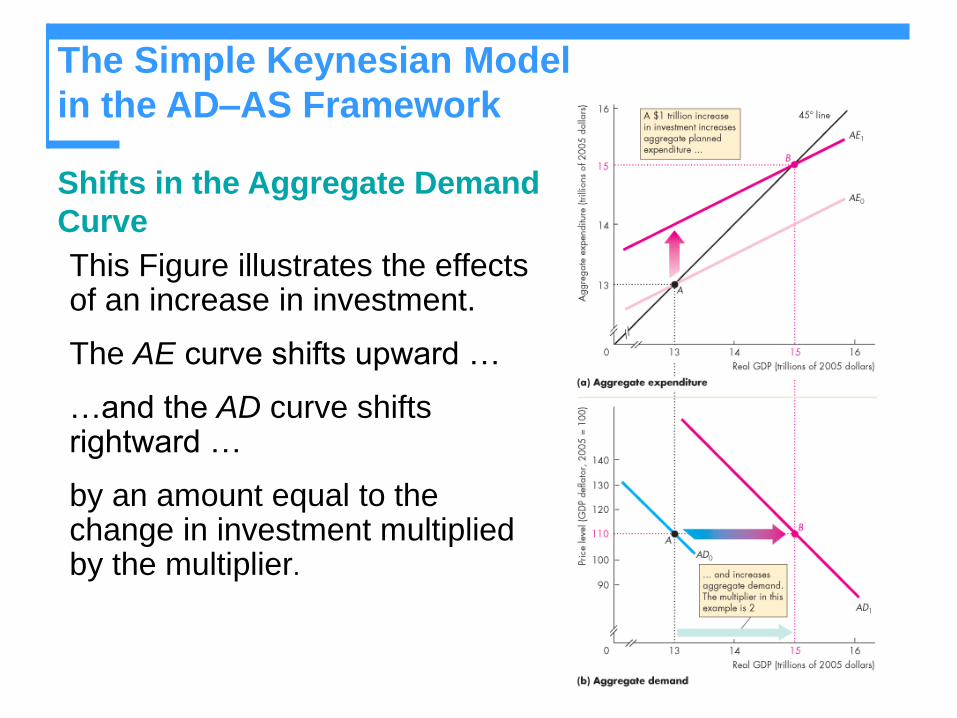
This Figure illustrates the effects of an increase in investment.
The AE curve shifts upward …
…and the AD curve shifts rightward …
by an amount equal to the change in investment multiplied by the multiplier.
The Simple Keynesian Model in the AD–
AS Framework
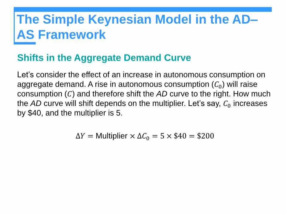
Shifts in the Aggregate Demand Curve
Let’s consider the effect of an increase in autonomous consumption on
aggregate demand. A rise in autonomous consumption (𝐶0) will raise
consumption (𝐶) and therefore shift the AD curve to the right. How much
the AD curve will shift depends on the multiplier. Let’s say, 𝐶0 increases
by $40, and the multiplier is 5.
∆𝑌 = Multiplier × ∆𝐶0 = 5 × $40 = $200
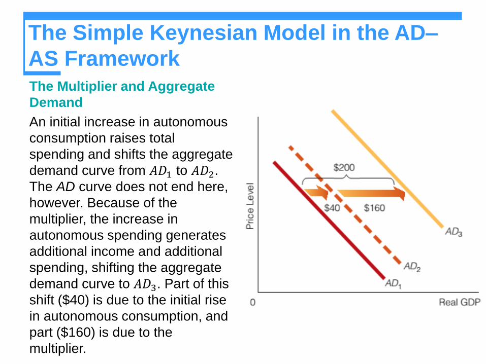
The Simple Keynesian Model in the AD–
AS FrameworkThe Multiplier and Aggregate
Demand
An initial increase in autonomous
consumption raises total
spending and shifts the aggregate
demand curve from 𝐴𝐷1 to 𝐴𝐷2. The AD curve does not end here,
however. Because of the
multiplier, the increase in
autonomous spending generates
additional income and additional
spending, shifting the aggregate
demand curve to 𝐴𝐷3. Part of this
shift ($40) is due to the initial rise
in autonomous consumption, and
part ($160) is due to the
multiplier.
The Simple Keynesian Model in the AD–
AS Framework
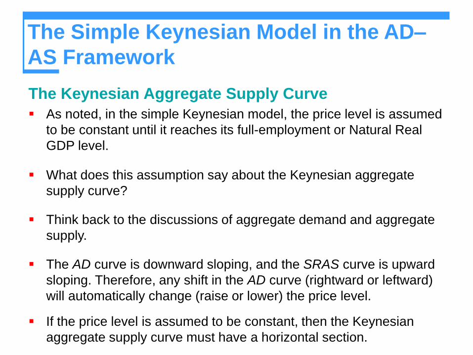
The Keynesian Aggregate Supply Curve
As noted, in the simple Keynesian model, the price level is assumed
to be constant until it reaches its full-employment or Natural Real
GDP level.
What does this assumption say about the Keynesian aggregate
supply curve?
Think back to the discussions of aggregate demand and aggregate
supply.
The AD curve is downward sloping, and the SRAS curve is upward
sloping. Therefore, any shift in the AD curve (rightward or leftward)
will automatically change (raise or lower) the price level.
If the price level is assumed to be constant, then the Keynesian
aggregate supply curve must have a horizontal section.
The Simple Keynesian Model in the AD–
AS Framework
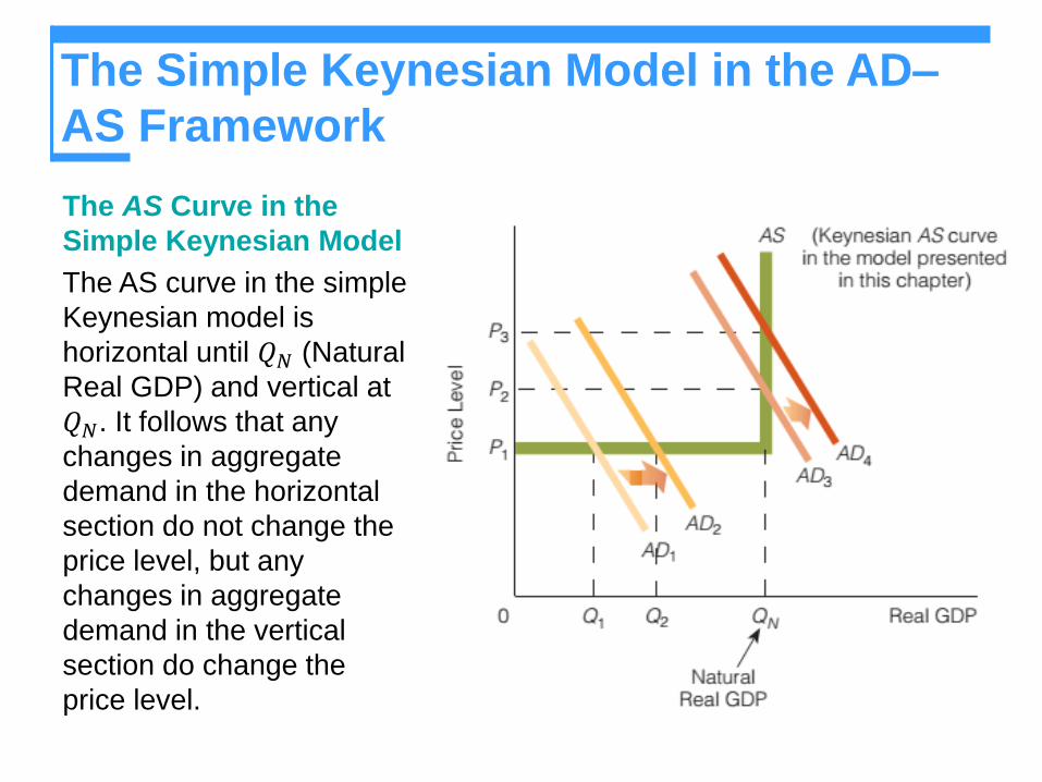
The AS Curve in the
Simple Keynesian Model
The AS curve in the simple
Keynesian model is
horizontal until 𝑄𝑁 (Natural
Real GDP) and vertical at
𝑄𝑁. It follows that any
changes in aggregate
demand in the horizontal
section do not change the
price level, but any
changes in aggregate
demand in the vertical
section do change the
price level.
The Simple Keynesian Model in the AD–
AS Framework
The AS Curve in the
Simple Keynesian Model
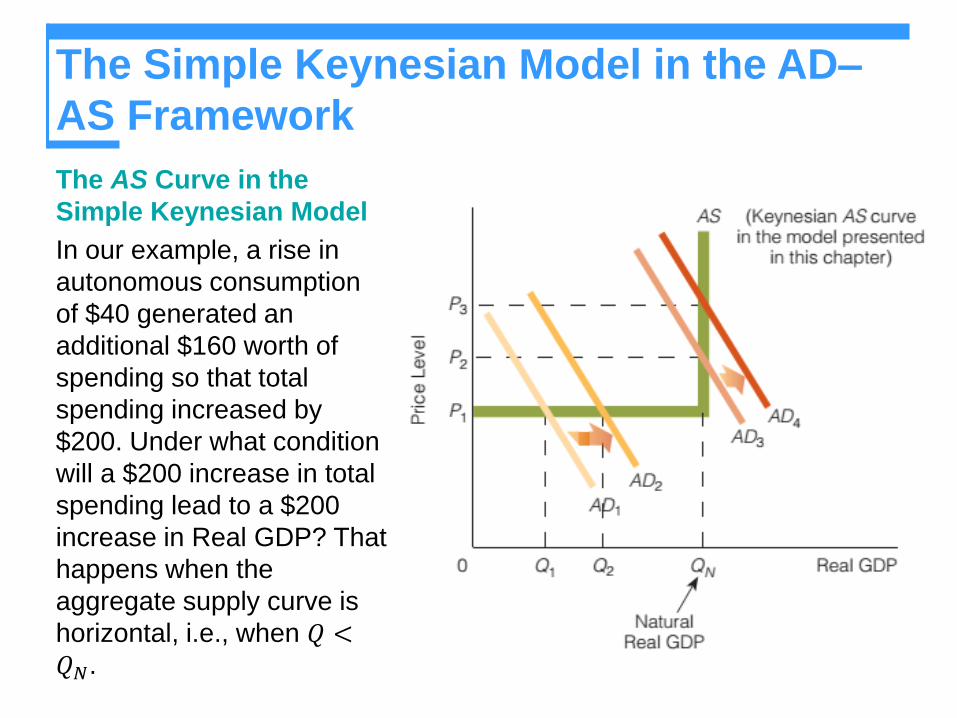
In our example, a rise in
autonomous consumption
of $40 generated an
additional $160 worth of
spending so that total
spending increased by
$200. Under what condition
will a $200 increase in total
spending lead to a $200
increase in Real GDP? That
happens when the
aggregate supply curve is
horizontal, i.e., when 𝑄 <𝑄𝑁.
The Simple Keynesian Model in the AD–
AS Framework
The AS Curve in the
Simple Keynesian
Model
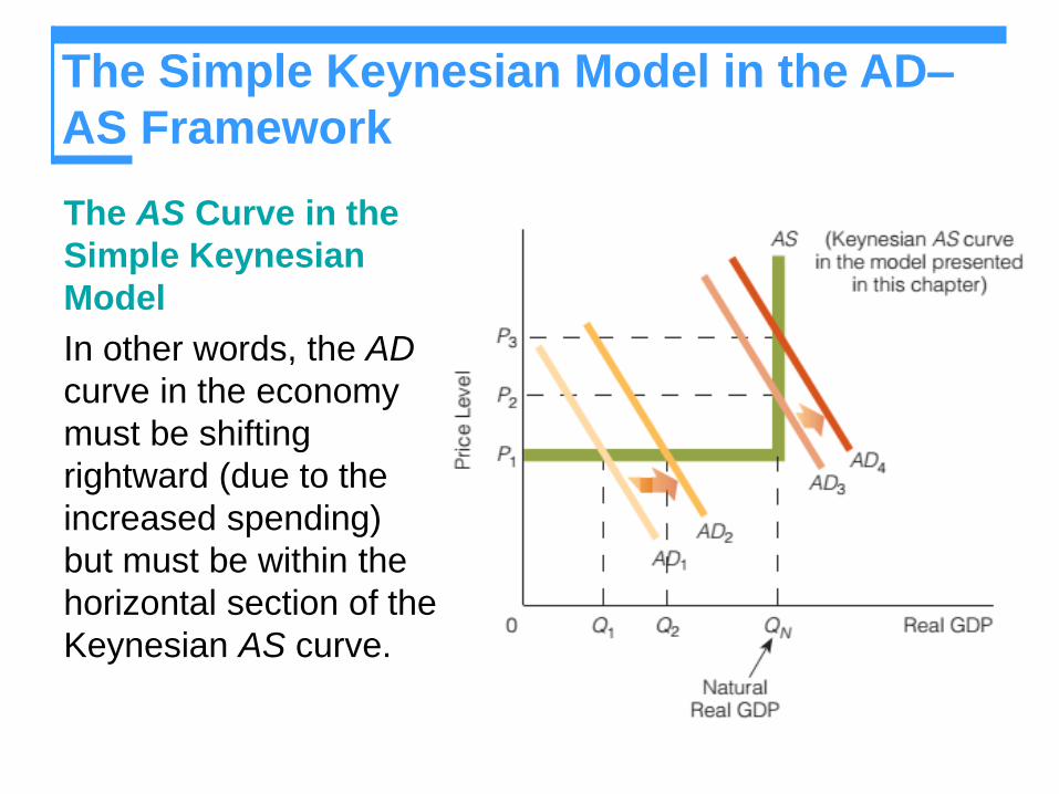
In other words, the AD
curve in the economy
must be shifting
rightward (due to the
increased spending)
but must be within the
horizontal section of the
Keynesian AS curve.
The Simple Keynesian Model in the AD–
AS Framework
The Economy in a
Recessionary Gap
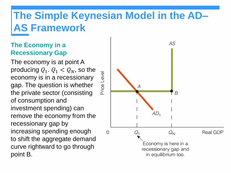
The economy is at point A
producing 𝑄1. 𝑄1 < 𝑄𝑁, so the
economy is in a recessionary
gap. The question is whether
the private sector (consisting
of consumption and
investment spending) can
remove the economy from the
recessionary gap by
increasing spending enough
to shift the aggregate demand
curve rightward to go through
point B.
The Simple Keynesian Model in the AD–
AS Framework
The Economy in a
Recessionary Gap
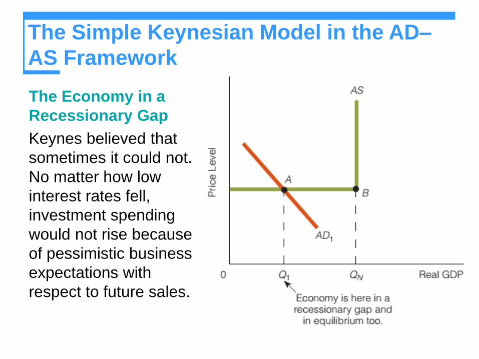
Keynes believed that
sometimes it could not.
No matter how low
interest rates fell,
investment spending
would not rise because
of pessimistic business
expectations with
respect to future sales.
The Simple Keynesian Model in the AD–
AS Framework
Government’s Role in the Economy
In the self-regulating economy of the classical economists,
government does not have a management role to play. The
private sector (households and businesses) is capable of self-
regulating the economy at its Natural Real GDP level.
On the other hand, Keynes believed that the economy is not
self-regulating and that economic instability is a possibility. In
other words, the economy could get stuck in a recessionary gap.
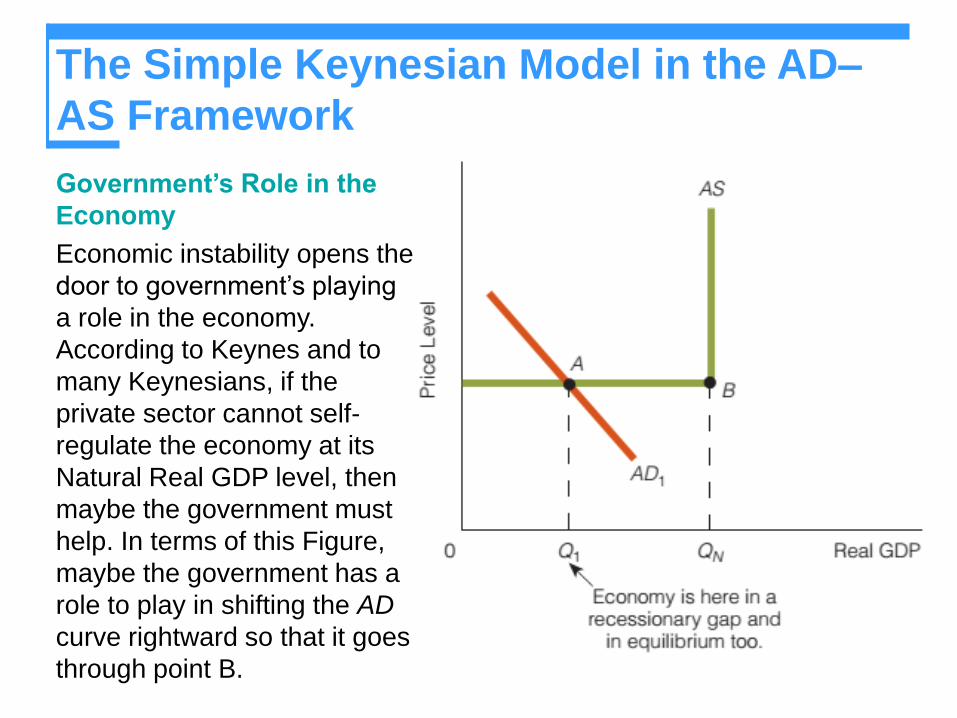
The Simple Keynesian Model in the AD–
AS Framework
Government’s Role in the
Economy
Economic instability opens the
door to government’s playing
a role in the economy.
According to Keynes and to
many Keynesians, if the
private sector cannot self-
regulate the economy at its
Natural Real GDP level, then
maybe the government must
help. In terms of this Figure,
maybe the government has a
role to play in shifting the AD
curve rightward so that it goes
through point B.
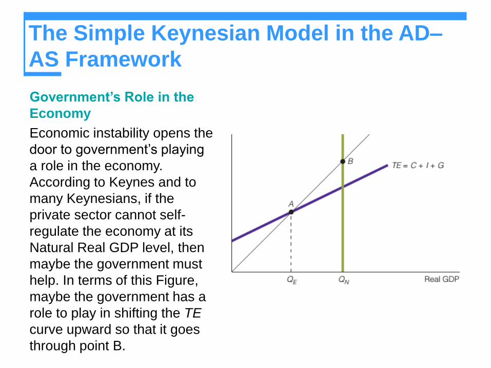
Government’s Role in the
Economy
Economic instability opens the
door to government’s playing
a role in the economy.
According to Keynes and to
many Keynesians, if the
private sector cannot self-
regulate the economy at its
Natural Real GDP level, then
maybe the government must
help. In terms of this Figure,
maybe the government has a
role to play in shifting the TE
curve upward so that it goes
through point B.
The Simple Keynesian Model in the AD–
AS Framework
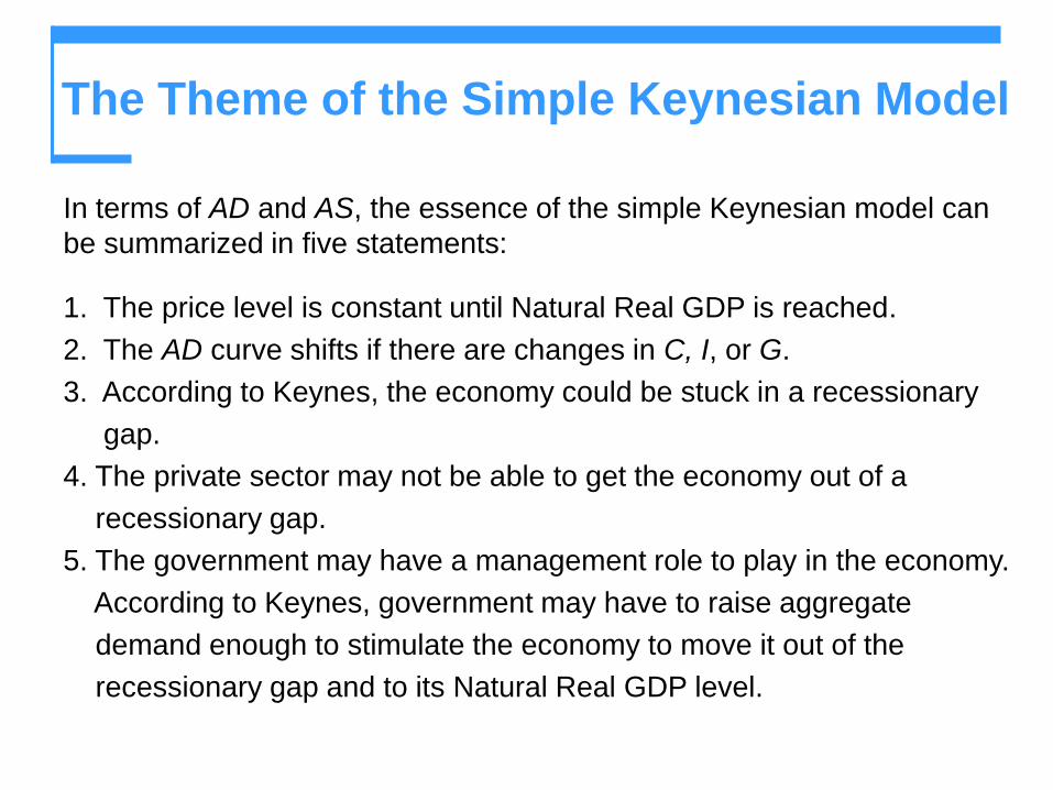
The Theme of the Simple Keynesian Model
In terms of AD and AS, the essence of the simple Keynesian model can
be summarized in five statements:
1. The price level is constant until Natural Real GDP is reached.
2. The AD curve shifts if there are changes in C, I, or G.
3. According to Keynes, the economy could be stuck in a recessionary
gap.
4. The private sector may not be able to get the economy out of a
recessionary gap.
5. The government may have a management role to play in the economy.
According to Keynes, government may have to raise aggregate
demand enough to stimulate the economy to move it out of the
recessionary gap and to its Natural Real GDP level.
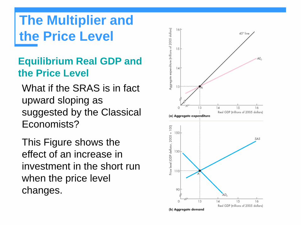
The Multiplier and
the Price Level
Equilibrium Real GDP and
the Price Level
What if the SRAS is in fact
upward sloping as
suggested by the Classical
Economists?
This Figure shows the
effect of an increase in
investment in the short run
when the price level
changes.
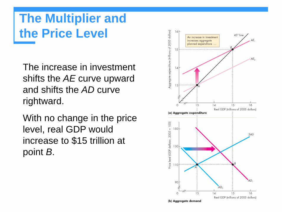
The Multiplier and
the Price Level
The increase in investment
shifts the AE curve upward
and shifts the AD curve
rightward.
With no change in the price
level, real GDP would
increase to $15 trillion at
point B.
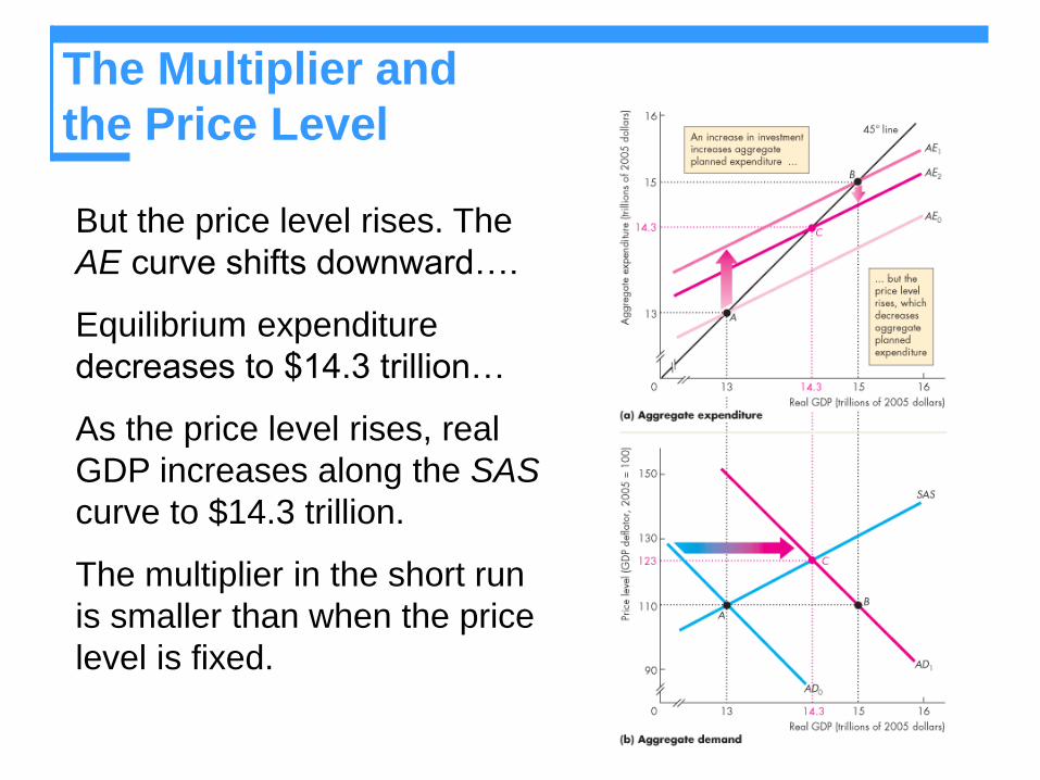
The Multiplier and
the Price Level
But the price level rises. The
AE curve shifts downward….
Equilibrium expenditure
decreases to $14.3 trillion…
As the price level rises, real
GDP increases along the SAS
curve to $14.3 trillion.
The multiplier in the short run
is smaller than when the price
level is fixed.
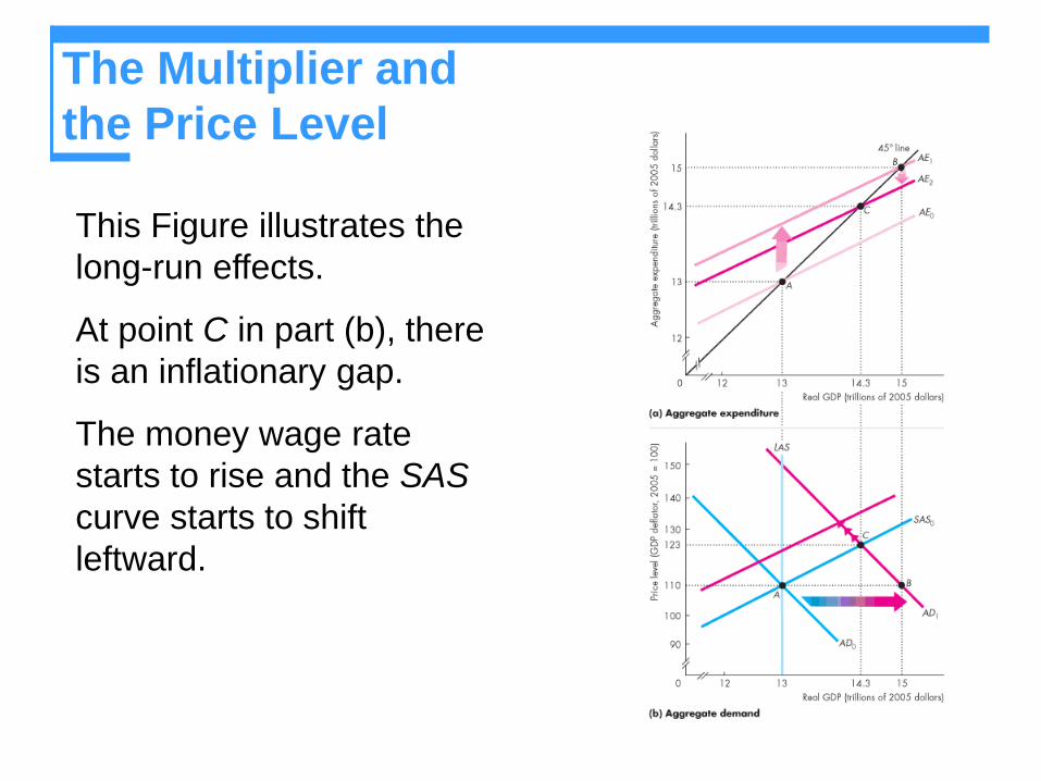
The Multiplier and
the Price Level
This Figure illustrates the
long-run effects.
At point C in part (b), there
is an inflationary gap.
The money wage rate
starts to rise and the SAS
curve starts to shift
leftward.
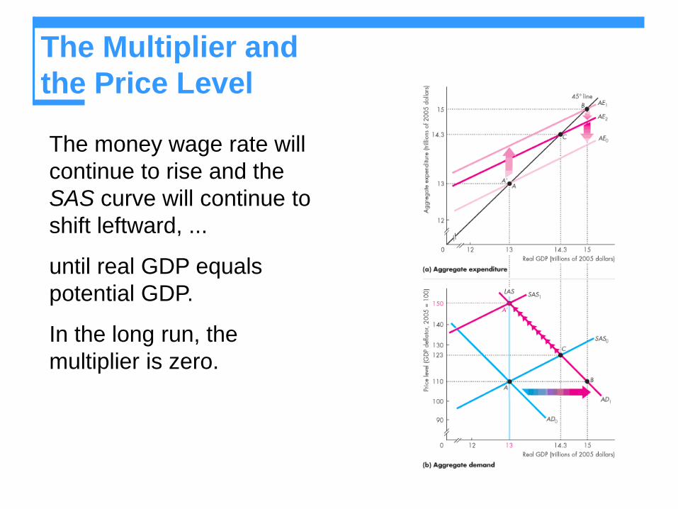
The Multiplier and
the Price Level
The money wage rate will
continue to rise and the
SAS curve will continue to
shift leftward, ...
until real GDP equals
potential GDP.
In the long run, the
multiplier is zero.