Stereotypes

Pedro Bordalo, Katherine Coffman, Nicola Gennaioli, Andrei Shleifer∗

First draft, November 2013. This version, May 2015.

Abstract

We present a model of stereotypes in which a decision maker assessing a group recalls

only that group’s most representative or distinctive types. Stereotypes highlight differences

between groups, and are especially inaccurate (consisting of unlikely, extreme types) when

groups are similar. Stereotypical thinking implies overreaction to information that generates

or confirms a stereotype, and underreaction to information that contradicts it. Stereotypes

can change if new information changes the group’s most distinctive trait. We present exper-

imental evidence on the role of representativeness in shaping subjects’ mental representation

of groups.

∗Royal Holloway University of London, Ohio State University, Universitá Bocconi and IGIER, HarvardUniversity. We are grateful to Nick Barberis, Roland Bénabou, Dan Benjamin, Tom Cunningham, MatthewGentzkow, Emir Kamenica, Larry Katz, David Laibson, Sendhil Mullainathan, Josh Schwartzstein, JesseShapiro, Alp Simsek and Neil Thakral for extremely helpful comments. We thank the Initiative on Founda-tions of Human Behavior for support of this research.

1 Introduction

The Oxford English Dictionary defines a stereotype as a “widely held but fixed and oversim-

plified image or idea of a particular type of person or thing”. Stereotypes are ubiquitous.

Among other things, they cover racial groups (“Asians are good at math”), political groups

(“Republicans are rich”), genders (“Women are bad at math”), demographic groups (“Florida

residents are elderly”), and activities (“flying is dangerous”). As these and other examples

illustrate, some stereotypes are roughly accurate (“the Dutch are tall”), while others much

less so (“Irish are red-headed”; only 10% are). Moreover, stereotypes change: in the US, Jews

were stereotyped as religious and uneducated at the beginning of the 20th century, and as

high achievers at the beginning of the 21st (Madon et. al., 2001).

Social science has produced three broad approaches to stereotypes. The economic ap-

proach of Phelps (1972) and Arrow (1973) sees stereotypes as a manifestation of statistical

discrimination: rational formation of beliefs about a group member in terms of the aggregate

beliefs about that group. Statistical discrimination may impact actual group characteristics

in equilibrium (Arrow 1973). For example, if employers hold adverse beliefs about the skills

of black workers, blacks would underinvest in education, thereby fulfilling the adverse prior

beliefs. However, because in this theory stereotypes are based on rational expectations, it

does not address a central problem that stereotypes are often inaccurate. The vast majority

of Florida residents are not elderly, the vast majority of the Irish are not red-headed, and

flying is really pretty safe.

The sociological approach to stereotyping pertains only to social groups. It views stereo-

types as fundamentally incorrect and derogatory generalizations of group traits, reflective of

the stereotyper’s underlying prejudices (Adorno et al. 1950) or other internal motivations

(Schneider 2004). Social groups that have been historically mistreated, such as racial and

ethnic minorities, continue to suffer through bad stereotyping, perhaps because the groups

in power want to perpetuate false beliefs about them (Steele 2010, Glaeser 2005). The

stereotypes against blacks are thus rooted in the history of slavery and continuing discrim-

ination. This approach might be relevant in some important instances, but it leaves a lot

out. While some stereotypes are inaccurate, many are quite fair (“Dutch are tall,” “Swedes

1

are blond.”) Moreover, many stereotypes are flattering to the group in question rather than

pejorative (“Asians are good at math”). Finally, stereotypes change, so they are at least in

part responsive to reality rather than entirely rooted in the past (Madon et. al., 2001)

The third approach to stereotypes – and the one we follow – is the “social cognition

approach”, rooted in social psychology (Schneider 2004). This approach gained ground in

the 1980s and views social stereotypes as special cases of cognitive schemas or theories

(Schneider, Hastorf, and Ellsworth 1979). These theories are intuitive generalizations that

individuals routinely use in their everyday life, and entail savings on cognitive resources.1

Hilton and Hippel (1996) stress that stereotypes are “mental representations of real differences

between groups [. . . ] allowing easier and more efficient processing of information. Stereotypes

are selective, however, in that they are localized around group features that are the most

distinctive, that provide the greatest differentiation between groups, and that show the least

within-group variation.” A related “kernel-of-truth hypothesis” holds that stereotypes are

based on some empirical reality; as such, they are useful, but may entail exaggerations

(Judd and Park 1993).

To us, this approach to stereotypes seems intimately related to another idea from psy-

chology: the use of heuristics in probability judgments (Kahneman and Tversky 1972). Just

as heuristics simplify the assessment of complex probabilistic hypotheses, they also simplify

the representation of heterogeneous groups. In this way, heuristics enable a quick and often

reliable assessment of complex situations, but sometimes cause biases in judgments. Consider

in particular the representativeness heurstic. Kahneman and Tversky (1972) write that “an

attribute is representative of a class if it is very diagnostic; that is, the relative frequency of

this attribute is much higher in that class than in the relevant reference class.” Representa-

tiveness suggests that the reason people stereotype the Irish as red-headed is that red hair is

more common among the Irish than among other groups, even though it is not that common

in absolute terms. The reason people stereotype Republicans as wealthy is that the wealthy1In the words of Lippmann (1922, pp.88-89), an early precursor of this approach: “There is economy

in this. For the attempt to see all things freshly and in detail, rather than as types and generalities, isexhausting, and among busy affairs practically out of the question[. . . ]. But modern life is hurried andmultifarious, above all physical distance separates men who are often in vital contact with each other, suchas employer and employee, official and voter. There is neither time nor opportunity for intimate acquaintance.Instead we notice a trait which marks a well-known type, and fill in the rest of the picture by means of thestereotypes we carry about in our heads.”

2

are more common among Republicans than Democrats.2 In both cases, the representation

entails judgment errors: people overestimate the proportion of red-haired among the Irish, or

of the wealthy among the Republicans. Representativeness thus generates stereotypes that

differentiate groups along existing and highly diagnostic characteristics, exactly as Hilton,

Hippel and Schneider define them.3 While representativeness is not the only heuristic that

shapes recall (availability, driven by recency or frequency of exposure, also plays a role), it

is the key driving force of stereotypes which, in line with the social psychology perspective,

are centered on differences among groups.4

In this paper, we systematically explore the connection between the representativeness

heuristic and the social psychology view of stereotypes as intuitive generalizations. Our anal-

ysis uses the definition of representativeness from Gennaioli and Shleifer (2010), although the

application here is different from the issues analyzed in that paper. Formally, we assume that

a type t is representative for group G if it is diagnostic of G relative to a comparison group

−G, in that the diagnostic ratio Pr(G|t)/Pr(−G|t) is high. Equivalently, a representative

type for group G has a high likelihood ratio:

Pr(t|G)

Pr(t| −G). (1)

Due to limited working memory, the most representative types come to mind first and are

overweighted in judgments. We assume that the stereotype of G contains only the d ≥ 1

most representative types according to (1). Non-representative types do not come to mind

and are neglected. Predictions about G are then made by conditioning the true distribution

Pr(t|G) to the group’s most representative types (our results go through with a smoother

discounting of the probability of less representative types).

The critical feature of our approach is that representativeness, and stereotypes, can only2See www.nytimes.com/packages/pdf/politics/20041107_px_ELECTORATE.xls.3Deaux and Kite (1985) stress that the features that distinguish a category from a comparison category

are especially useful as identifying characteristics. According to Schneider (2004 p. 91), the stereotype fora category should have “membership diagnosticity”: “all females have hearts (feature diagnosticity), but notall people who have hearts are female (membership diagnosticity). Similarly, membership diagnosticity canbe nearly perfect, but feature diagnosticity may still be quite low; people who nurse babies are female, butfar from all females are nursing at any given time[. . . ] Hearts won’t do the job for femaleness, but possessionof a uterus works.”

4See Section 3.2 and Appendix C for an in depth discussion of these issues.

3

exist in context, that is, relative to a comparison group −G. This implies that, as the

comparison group changes, so do representativeness, stereotypes, and assessments. In Section

2, as a motivation for our analysis, we present experimental evidence supportive of this key

prediction. We construct a group of mundane objects, G, and present it to participants

next to a comparison group, −G. In our baseline condition, the comparison group is chosen

so that no type is particularly representative of group G. In our treatment, we change the

comparison group, −G, while leaving the target group, G, unchanged. The new comparison

group gives rise to highly representative types within G. In line with the key prediction of

our model, participants in the treatment condition shift their assessment of G toward the

new representative types.

We next turn to the analysis of the model. To give a preview of some of our results, we

find that representativeness often generates fairly accurate stereotypes but sometimes causes

stereotypes to be inaccurate, particularly when groups have similar distributions that differ

most in unlikely types. To illustrate this logic, consider the formation of the stereotype

“Florida residents are elderly”. The proportion of elderly people in Florida and in the overall

US population is shown in the table below.5

age 0− 18 19− 44 45− 64 65+

Florida 23.9% 31.6% 27.0% 17.3%

US 26.6% 33.4% 26.5% 13.5%

The table shows that the age distributions in Florida and in the rest of the US are

very similar. Yet, someone over 65 is highly representative of a Florida resident, because

this age bracket maximizes the likelihood ratio Pr(t|Florida)/Pr(t|US).6 When thinking

about the age of Floridians, then, the “65+” type immediately comes to mind because in

this age bracket Florida is most different from the rest of the US, in the precise sense of

representativeness. Representativeness-based recall induces an observer to overweight the

“65+” type in his assessment of the average age of Floridians.

Critically, though, this stereotype is inaccurate. Indeed, and perhaps surprisingly, only5See http://quickfacts.census.gov/qfd/states/12000.html.6In this problem, the likelihood ratio in (1) is Pr(t|Florida)/Pr(t|rest of US), but it is easy to see that t

maximizes Pr(t|Florida)/Pr(t|rest of US) if and only if it maximizes Pr(t|Florida)/Pr(t|US).

4

about 17% of Florida residents are elderly. The largest share of Florida residents, nearly

as many as in the overall US population, are in the age bracket “19-44”, which maximizes

Pr(t|Florida). Being elderly is not the most likely age bracket for Florida residents, but

rather the age bracket that occurs with the highest relative frequency. A stereotype-based

prediction that a Florida resident is elderly has very little validity.

Besides offering guidance on the circumstances in which stereotypes are more or less

accurate, our model has many other implications. In particular:

• Stereotypes amplify systematic differences between groups, even if these differences are

in reality very small. When groups differ by a shift in means, stereotyping exaggerates

differences in means, and when groups differ by a increase in variance, stereotyping

exaggerates the differences in variances. In these cases (though not always), represen-

tativeness yields stereotypes that contain a “kernel of truth”.

• Stereotypes are context dependent. The assessment of a given target group depends

on the group to which it is compared. For instance, when comparing Irish to Scots,

the stereotype of Irish may change from “red-haired” to “Catholic”. In particular, when

types are defined by several dimensions, stereotypes are formed along the dimension

in which groups differ the most.

• Stereotypes distort reaction to information. So long as stereotypes do not change, peo-

ple under-react or even ignore information inconsistent with stereotypes. If however

enough contrary information is received (e.g. observing more women than men succeed-

ing at math) stereotypes change, leading to a drastic reevaluation of already available

data. Representativeness-based recall reconciles under-reaction with over-reaction to

data, generating both confirmation bias and base-rate neglect.

Although we have argued that stereotypes, like heuristics, allow for quick and often useful

assessments, they are not always benign. Some of the errors caused by inaccurate stereo-

types are inconsequential. A driver being cut off on the road might form a quick gender or

age stereotype of the aggressor, but then quickly drive on and forget about it. But stereo-

typical thinking can also have substantial consequences. One instance, discussed in Section

5

4.2, concerns the role of gender stereotypes in mathematics or occupational choice (Buser

et al (2014)). Similarly, graduate admission officers scanning dozens of files might reject

foreign candidates who bring to mind ethnic stereotypes and accept potentially less talented

candidates with A’s from Ivy League schools. We do not suggest that decision makers are

uniformly bound to stereotypical thinking in all situations; rather that it requires substantial

cost and deliberation to enrich one’s mental representations, and even deliberation may not

fully overcome the influence of stereotypes.

Since Kahneman and Tversky’s (1972, 1973) work on heuristics and biases, several studies

have formally modelled heuristics about probabilistic judgments and incorporated them into

economic models. Work on the confirmation bias (Rabin and Schrag 1999) and on proba-

bilistic extrapolation (Grether 1980, Barberis, Shleifer, and Vishny 1998, Rabin 2002, Rabin

and Vayanos 2010, Benjamin, Rabin and Raymond 2011) assumes that the decision maker

has an incorrect model in mind or incorrectly processes available data. Our approach is

instead based on the single assumption that only representative information comes to mind

when making judgments. The specific mental operation that lies at the heart of our model

– namely, generating a prediction for the distribution of types in a group, based on data

stored in memory – also captures instances of base-rate neglect and confirmation bias as

described above. Gennaioli and Shleifer (2010) show that representativeness based thinking

can account for other well-known violations of the laws of probability, including the well

known conjunction bias (the “Linda” problem) and disjunction bias.7

In the next section, we present suggestive experimental evidence on the role of represen-

tativeness in recall-based judgments. Section 3 describes our model. In Section 4 we examine

the properties of stereotypes, including the forces that shape stereotype accuracy. In Section

5, we describe how stereotypes can cause both under- and over-reaction to new information.

Section 6 concludes. Appendix A contains the proofs. In Appendix B we consider the case

of unordered types, in Appendix C we extend the model to account for the role of likelihood7The neglect of information in our model simplifies judgment problems in a way related to models of

categorization (Mullainathan 2002). In these models, however, decision makers use coarse categories or-ganized according to likelihood, not representativeness. This approach generates imprecision but does notcreate a systematic bias for overestimating unlikely events, nor does it allow for a role of context in shapingassessments. Our emphasis on representative and distinctive features or types is also related to research onsalience (BGS 2012, 2013).

6

and availability in recall, and in Appendix D we extend the analysis to the cases where types

are continuous. In Appendix E we present the full details and analysis of our experiments.

2 Motivating Evidence on Group Assessment

The assumption of representativeness-based recall implies that assessments of groups are

made in contrast to, and emphasize differences with, comparison groups. Assessments are

therefore context dependent, in the sense that judgements about a group depend on the

features of the group it is compared to. We assess this prediction in a controlled laboratory

environment. While field evidence on widely-held stereotypes is suggestive, the laboratory

setting allows us to isolate the role of representativeness, abstracting from many other factors

– historical, sociological, or otherwise – that may also play a role in stereotype formation. We

construct our own groups of ordinary objects, creating a target group, G, and a comparison

group, −G. We explore how participant impressions of G change as we vary the represen-

tativeness of different types within this target group simply by changing the comparison

group.

We conducted several experiments, in the laboratory as well as on Amazon Mechanical

Turk. Each involves a basic three-step design. First, participants are shown the target group

and a randomly-assigned comparison group for 15 seconds. In this time frame, differences

across the groups can be noticed but the groups’ precise compositions cannot be memorized.

The second step consists of a few filler questions, that briefly draw the participants’ cognitive

bandwidth away from their observation. Finally, participants are asked to recall the groups

they saw, and assess them in various ways. Participants are incentivized to provide accurate

answers.

We randomly assign participants to either the Control or the Representativeness condi-

tion. In the Control condition, G and −G have nearly identical distributions, so that all

types are equally representative for each group. In the Representativeness condition, G is

unchanged, while the composition of the comparison group −G is changed in such a way

that a certain type becomes very representative for G. Context dependence implies that the

assessment of G should now overweight this representative type, even though the distribution

7

of G itself has not changed.

We ran six experiments of this form, with design changes focused on reducing participant

confusion and removing confounds. Here, we describe the final, and most refined, versions

of these experiments. In an attempt to provide a overview of the results while remaining

concise, we also provide the results from pooled specifications that use all data collected. In

Appendix E, we present additional details and report all experiments conducted. We also

provide instructions and materials for each experiment and the full data set.

Consider first the experiment illustrated in Figure 1. A group of 25 cartoon girls is

presented next to a group of 25 cartoon boys in t-shirts of different colors: blue, green,

or purple. In the Control condition, Fig.1a, the groups have identical color distributions

(13 purple, 12 green), so no color is representative of either group. The Representativeness

condition, Fig.1b, compares the same group of girls with a different group of boys, for

whom green shirts are replaced by blue shirts. Now only girls wear green and only boys

wear blue. These colors, while still not the most frequent for either group, are now most

representative. For each group, girls and boys, participants are asked to identify the modal

color shirt worn by that group. Our key prediction is that when the less frequent color (the

12-shirt color) is representative for a group, participants will be more likely to believe it

to be modal for that group. Note that the only factor that varies across treatments is the

representativeness of the 12-color shirt. Thus, if we see differences across conditions, the

causal role of representativeness-based recall in shaping group judgments is clear.8

We collected data from 301 participants using this T-shirts design.9 Consistent with the

role of representativeness, participants assigned to the Representativeness condition are 10.5

percentage points more likely to recall the less frequent color (blue or green) as the modal

color when it is representative of a group (35% of participants guess the less frequent color is

modal in the Control condition, this proportion increases to 46% in the Representativeness8Note that we vary which colors are used in which roles across participants – that is, some participants

saw this particular color distribution, while others see, for example, green as the modal color, with purpleas the diagnostic color for boys in the Rep. condition and blue as the diagnostic color for girls in the Rep.condition. We vary the colors across the roles to avoid confounding the characteristics of any particular colorwith its diagnosticity.

9Throughout our analysis, we exclude any participant who participated in a previous version of theexperiment and any participant who self-identified as color blind. In Appendix E, we show that our resultsare unchanged if we include these additional observations.

8

(a) Control Condition (b) Representativeness Condition

Figure 1: T-shirts Experiment

condition, p=0.01, estimated from a probit regression reported in Appendix E). We also ask

participants to estimate how many of each color T-shirts they saw in each group. In both

treatments, the true difference in counts is one (13 purple shirts, 12 green or blue shirts). In

the Control condition, participants on average believe they saw 0.54 more purple shirts than

green or blue shirts, while in the Representativeness condition, participants believe they saw

0.72 fewer purple shirts than green or blue shirts (across treatment difference is significant

with p=0.013 from two-tailed Fisher Pitman permutation test).

The next experiment, illustrated in Figure 2, shows that the effect survives even when

the representative types are much less frequent, or in the tails. Groups are sets of 24 ice

cream cones: group membership is defined by ice cream flavor (chocolate vs strawberry),

and types are the number of ice cream scoops, ranging from 1 to 5. In the Control condition,

Fig.2a, distributions are very similar, with most cones having intermediate numbers (2 or

3) of scoops. Here, no type is particularly representative of either group. In the representa-

tiveness condition, Fig.2b, the same chocolate cones are presented next to a different group

of strawberry cones. In the Representativeness condition, strawberry cones have the same

average number of scoops as do the Control condition strawberry cones, but, importantly,

they do not contain any 5-scoop cones. This makes the right tail, 5-scoop cones very repre-

sentative for the chocolate group. Similarly, in this condition only the strawberry group has

a cone with 1 scoop, making the left tail very representative for that group.

We collected data from 223 participants using this design. Participants are asked which

9

(a) Control Condition (b) Representativeness Condition

Figure 2: Ice cream cone Experiment

flavor has more scoops on average. We use this binary question, rather than a more complex

elicitation of their recollection of entire distributions, because it is simple, easy to incentivize,

and should move with participants’ impressions of the distributions. In reality, strawberry

has a slightly higher average in both conditions (3.167 for strawberry versus 3.125 for choco-

late). Yet, and consistent with context dependence, we see a shift in the prediction direction

across condition. In the Control condition, 44% of participants incorrectly believe that the

chocolate scoops have more scoops on average; in the Representativeness condition, this mis-

take is made by 54% of participants (p=0.16 estimated from a two-tailed test of proportions).

We also ask participants (i) to estimate the average number of scoops in each group and (ii)

to make a choice between the two lotteries induced by the distributions of cones. We find

no significant differences across conditions for these questions.10

In total, we collected data for six experiments of this general structure, gathering evidence

from more than 1,000 participants. As we describe in Appendix E, while there is substantial

variation across experiments, when we pool all data collected we find significant aggregate

treatment effects in line with a role of representativeness in judgment (see Appendix E).11

Using a probit regression that pools all of the data for unordered type experiments similar

to the T-shirts experiment (four versions, 741 participants), we find that participants are10We describe these two questions in more detail in Appendix E. We conjecture that participant risk

preferences may have overwhelmed the role of representativeness-based recall in the lottery choice. Wediscuss this interpretation of this result, and provide supporting evidence, in Appendix E.

11We find effects in the predicted directions for all six designs, with significant effects for two. We discussthe extent to which our results are sensitive to the specifics of the design, in Appendix E.

10

9.3 percentage points more likely to guess that the less frequent type is modal when it is

representative than when it is not (p=0.002). For ordered type experiments similar to ice

cream cones (two versions, 402 participants), participants are 11.5 percentage points more

likely to guess that the group of interest has a greater average than the comparison group

when the right tail is representative (p=0.026).12 Given our simple experimental setting

with groups of mundane objects, we interpret our results – a significant and reasonably-sized

impact on average beliefs – as an important proof of concept: the presence of representative

types biases ex post assessment.

We next present the model of representativeness-based judgments that features the type

of context dependence observed in our experiments.

3 A Model of Representativeness and Stereotypes

3.1 The Model

A decision maker (DM) faces a prediction problem, which entails representing the distribution

of types t in a group G. The DM may be assessing the ability of a job candidate coming from

a certain ethnic group, the future performance of a firm belonging to a certain sector, or

his future earnings based on his own educational background. The DM solves this problem

by forming a simplified representation of G, which relies on recalling from memory only the

most representative types of group G relative to an alternative group −G.13

Formally, the DM must assess the distribution of a categorical random variable T in a

group G, which is a proper subset of the entire population Ω. The random variable T takes

values in a type space t1, . . . , tN that is naturally ordered, with t1 < . . . < tN (and in12Results for the ordered types experiments, unlike the simpler T-shirts style design, were sensitive to the

choice of platform, with consistently strong results on Amazon Mechanical Turk and weak or null results inlaboratory samples. We discuss this in Appendix E.

13Our model is concerned with the specific mental operation of recalling the conditional distribution oftypes t given G, which is stored in memory. We do not consider the related operation of inference, namelyof determining the probability that G vs −G is true. Gennaioli and Shleifer (GS 2010) offer a model ofrepresentativeness-based inference, in which DMs assess a hypothesis by recalling only its most representativescenarios relative to the alternative hypothesis. In GS (2010), scenario t is more representative of hypothesisG against an alternative −G if, conditional on t, G is more likely to be true than −G. This is closely relatedto our Definition 1 below.

11

many examples is assumed to be cardinal). In the examples of the introduction, G is men,

or Florida residents, or firms, while types are ability at mathematics, age, or stock returns.14

We denote by πt,G the true conditional probability Pr(T = t|G) of type t in group G and by

πt the true unconditional probability Pr(T = t) of type t in Ω.

The DM has stored in memory the full conditional distribution (πt,G)t∈t1,...,tN, but he

assesses this distribution by recalling only a limited and selected set of types. Selective recall

is driven by representativeness, formalized below following GS (2010).

Definition 1 The representativeness of type t for group G is defined as R(t, G) = Pr(G|T =

t)/Pr(−G|T = t), where −G = Ω\G. Bayes’ rule implies that representativeness increases

in the likelihood ratio:Pr(T = t|G)

Pr(T = t| −G)=

πt,Gπt,−G

. (2)

In line with Kahneman and Tversky’s (1972) intuition, a type t is representative of G if it

is relatively more likely to occur in G than in −G. When thinking about the age distribution

of Floridians, our minds find it easy to retrieve those age brackets that are relatively more

common in Florida, as compared to the rest of the US population. These types are diagnostic

of the target group: a type t is representative of group G if, after observing t, a Bayesian

DM is more confident that the type is drawn from G relative to its complement −G.

Definition 1 implies that DMs are attuned to log differences in probabilities. In particular,

a type is more representative for group G the more likely it is to occur under G relative to its

comparison group. Holding fixed πt,G, the larger is (πt,G − πt,−G), the more representative a

type is for G. At the same time, representativeness captures a form of diminishing sensitivity,

whereby, for fixed probability difference, a type is more likely to be recalled if it is unlikely

in the comparison group, namely when πt,−G is low.15 In fact, types that are unlikely in −G

can be very diagnostic for G.14The model applies also to cases in which types are not ordered, representing for instance occupations, or

when they are multi-dimensional, capturing a bundle of attributes such as occupation and nationality. Wereturn to these possibilities in Appendix B and Section 4.3 respectively. Also, G may represent any categoryof interest, such as the historical performance of a firm or industry, actions available to a decision maker(T = set of payoffs, G = occupations), or categories in the natural world (T = ability to fly, G = birds).

15This feature of our definition of representativeness links to Weber’s law of sensory perception, see Section4.4. It also links to our previous work on salience, in which we postulated that log differences in payoffs

12

The ease of recall of highly representative types affects judgments because recall is limited,

in that the DM recalls only the d < N most representative types. The DM’s assessment of

the distribution of types over G works as follows.

Definition 2 Denote by r ∈ 1, . . . , N the representativeness ranking of types (where ties

are sequentially ranked), and denote by t(r) the r-th most representative type for G. The

DM forms his beliefs according to the modified probability distribution:

πstt(r),G =

πt(r),G∑d

r′=1 πt(r′),G, for r ∈ 1, . . . , d.

0 otherwise.. (3)

In the event of ties, for all r > d such that R(t(r), G) = R(t(d), G) the stereotype also

includes t(r). Hence, more than d types may be recalled.

Representativeness shapes which types are recalled and thus the DM’s predictions about

G.16 We call the distribution (πstt(r),G)r=1,...,d the stereotype for G (where st stands for stereo-

type). For simplicity, we also use the term stereotype in reference to the represented types,

t1, . . . , td. These types are at the “top of mind.” The (N − d) least representative types are

at the back of mind and are neglected by the DM. These less representative types are not

viewed as impossible; they are just assigned zero probability in the DM’s current thinking.

This formulation allows us to model surprises or reactions to zero probability events, which

we come back to in Section 5. The other properties of the model, however, continue to hold

under a smoother underestimation of the probability of non-representative types. Here we

adopt discontinuous discounting because of its simplicity. More generally, while neglect is a

critical manifestation of limited memory – in line with discontinuous discounting – smooth

discounting is perhaps more appropriate when the type space is small (e.g., in the T-shirts

experiment of Section 2).17

determine the attention paid to lottery payoffs BGS (2012) and goods’ attributes (BGS 2013). Equation (2)establishes the same principle for the domain of probabilities.

16The assumed tie breaking rule approximates the average stereotype held by a large population of agentsin which ties are resolved randomly. However, this rule is not central for our results. We could alternativelyassume that ties are resolved randomly in the formation of stereotypes.

17Formally, discounting can depend continuously on representativeness via a weighting functionδ(πt,G/πt,−G) that is increasing in the likelihood ratio (i.e., δ′(·) > 0). Then, the probability of type t

13

In the extreme case where d = 1, the DM recalls only group G’s most representative

type t(1), which following psychological theories of categorization we call the exemplar, and

assigns it probability πstt(1),G = 1. In less extreme, and perhaps more realistic cases, d > 1

and the stereotype of G includes the exemplar and some less representative types. When

thinking about the age of Floridians, people recall not only retired baby boomers but also

other working age adults.

Stereotypes depend on true probabilities. Equation (3) implies that, conditional on

coming to mind, the assessed odds ratios of any two types is consistent with the DM’s

experience and information. Past experience or information about types is stored in the

DM’s long-term memory and thus, conditional on coming to mind, shapes assessments. Since

past experiences or information may vary across individuals, our model allows for individual

heterogeneity in stereotypes, driven for instance by culture.

3.2 Discussion of Assumptions

In our model stereotypes are simplified mental representations of groups characterized by

limited and selective recall of those groups’ types. Recall is limited because not all types are

evoked from memory. Recall is selective because the types in the stereotype are the most

representative ones relative to a comparison group. Due to these features, stereotypes allow

individuals to form judgments that economize on cognitive resources and time but in some

cases are systematically biased. In the next section, we show that representativeness-based

recall generates the key features of stereotypes stressed in social psychology: namely, stereo-

types often highlight (and exaggerate) real differences between groups and are selectively

localised around the most distinctive features of the target group relative to other groups

(Hilton and Hippel 1996). In Section 4.4 we discuss whether such stereotypical thinking,

despite the distortions it may cause, can be efficiency-enhancing given cognitive limitations.

under the stereotype is defined to be:

πstt,G =

δ(πt,G/πt,−G) · πk,G∑k δ(πk,G/πk,−G) · πk,G

In this formulation, the probability of types that have a higher representativeness ratio is inflated. GSV (2014)use smooth discounting to model underweighting of risk in financial markets. In that paper, discountingexponentially accelerates as the types features a lower and lower rank in representativeness.

14

Before moving to the formal analysis, we note some properties and limitations of our

assumptions. First, we do not claim that representativeness is the only heuristic that shapes

recall. Decision makers may for instance find it easier to recall types that are sufficiently

likely. Another potentially important mechanism is availability, understood by Kahneman

and Tversky (1972) as the “ease” with which information comes to mind. This may capture

aspects such as recency and frequency of exposure, which might be independent of likelihood

or representativeness.18 In Appendix C we formally model a more general recall mechanism

driven by a combination of representativeness and likelihood of types. In this extension,

stereotypes are less extreme, consisting of those representative types that are sufficiently

likely. This model can offer a useful starting point to capture availability as well, even

though a full model of availability is beyond the scope of this paper. Even in this more general

setting, the influence of representativeness on recall is the driving force of stereotypes which,

in line with the social psychology perspective, are based on underlying differences among

groups. The experimental evidence in Section 2 also shows that representativeness alone can

generate systematic biases in a lab environment that controls for likelihood, exposure, and

other factors.

The second set of model-related issues concerns how to implement Definition 1 in appli-

cations, including specifying the set of types T and the comparison group −G considered by

the DM. A third issue, addressed in Definition 2, is how representativeness impacts beliefs

(in this case, via truncation).

Consider first the specification of the group G and of the type space T . Often, the

problem itself provides a natural specification of these features. This is the case in the

empirically important class of “closed end” questions, such as those used in surveys, which

provide respondents with a set of alternatives. This is also the case in our experiments of

Section 2. More generally, the problem solved by the decision maker – such as evaluating

the CV of a job applicant coming from a certain ethnic group – primes both a group and a

set of types, such as the applicant’s qualification or skill. When, as we assume here, types18For instance, in the aftermath of the 9/11 terrorist attacks, and the ensuing media coverage, a US

respondent asked what Arabs are like might more easily recall terrorists than Bedouins, even when thereare vastly more Bedouins than terrorists among Arabs, and even though all Bedouins are Arabs, so thatBedouins are more representative of Arabs than terrorists.

15

have a natural order (such as income, age, education), the granularity of T is also naturally

given by the problem (income, age and years of schooling brackets). Where the set of types

is not specified by the problem, decision makers spontaneously generate one.19 Psychologists

have sought for years to construct a theory of natural types (Rosch 1998). We do not make

a contribution to this problem, but note that in many problems of interest in economics the

set of types is naturally given.20

Consider next the role of the comparison group −G. This group captures the context in

which a stereotype is formed and, again, is often implied by the problem: when G = Florid-

ians, −G =Rest of US population; when G = Black Americans, −G =White Americans. A

distinctive prediction of our model, confirmed by our experiments in Section 2, is that the

stereotype for a given group G depends on the comparison group −G. Shih et al (1999)

show that Asian-American women self-stereotype themselves as better or worse in math,

with corresponding impact on performance, when their ethnicity or gender, respectively, is

primed. When −G is not pinned down by the problem itself, to derive testable predictions

from representativeness, we set −G = Ω\G where Ω is the natural population over which

the unconditional distribution of types is measured.

In sum, although different ingredients may contribute to the formation of stereotypes,

of all these ingredients representativeness is the key assumption that generates stereotypes’

most central feature: highlighting differences between groups, even if these differences are

overwhelmed by their similarities, and even if the resulting beliefs are inaccurate.

4 Properties of Stereotypes

We now explore the characteristics of stereotypical beliefs and their accuracy. To mea-

sure accuracy of beliefs, we first consider the extent to which a stereotype’s distribution

(πstt,G)t=t1,...,tN is an accurate representation of the true distribution (πt,G)t=t1,...,tN . To do so,

19For example, suppose a person is asked to guess the typical occupation of a democratic voter in an “openended” format (without being provided with a set of alternatives). Here the level of granularity at whichtypes are defined is not obvious (e.g. teacher vs a university teacher vs a professor of comparative literature).

20Strictly speaking, granularity is also an issue when types are ordered. However, in contrast to non-ordered categories, in ordered categories distributions are typically smoother, so changing the bracketing hasminor effects on estimates.

16

we consider the quadratic loss function L =∑

t(πstt,G − πt,G)2. We also consider to what

extent the mean or the variance of the stereotypical distribution differs from the true mean

and variances. This test is appropriate for the distributions over cardinal types we consider.

4.1 Likely vs Unlikely Stereotypes

Using the quadratic loss function, a stereotype is accurate if the representative types it selects

are also the most likely types. In contrast, a stereotype is inaccurate if it selects the least

likely types. Equation (2) then yields the following characterization.

Proposition 1 Consider the distributions πt,G and πt,−G for G and −G.

i) If πt,G > πt′,G if and only if πt,−G > πt′,−G, for any t, t′ ∈ T , then the most represen-

tative type may coincide with the modal type for at most one group.

ii) If πt,G > πt′,G if and only if πt,−G < πt′,−G, for any t, t′ ∈ T , then each group’s most

representative type is its modal type.

Case i) says that representativeness tends to select inaccurate stereotypes for at least one

group when individuals compare groups that have similar distributions. Specifically, when

groups have the same modal types, representative differences occur in less likely types for at

least one group. Because representativeness focuses the DM on types for which the groups

are different, the DM fails to account for the fact that the groups are in fact quite similar.

Ethnic stereotypes based on crime or terrorism, for instance, exhibit this error: neglect

of the fact that by far the most common types in all groups are honest and peaceful. In

our laboratory findings, while the modal T-shirt color worn by both girls and boys in both

conditions was purple, participants were more likely to recall green or blue as the modal

color when this less frequent color was representative of the group.

Case ii) says that stereotypes tend to be accurate, in the sense that they select likely

types for both groups, when the distributions are very different, so that groups differ most

in their modes. The stereotype “Swedes are blond” is correct precisely because this trait

captures a majority of Swedes while it represents a minority trait in a comparison (e.g.,

European) population.

17

To see more clearly these implications of representativeness, suppose that the distribution

of types in group −G is a power transformation of that in G, namely πt,−G = π∗ · παt,G for

all t, where π∗ = 1/∑

t παt,G is a normalizing constant. If α > 0 , the likelihood ranking of

types for groups G and −G coincide: the two distributions are “similar” and in particular

have the same modal type. If instead α < 0, the distributions are very different because

the likelihood ranking of types for G is the opposite of that for −G. This parameterization

illustrates the results of Proposition 1:

Corollary 1 Let πt,−G = π∗ · παt,G as above. Then:

i) If α > 0, the stereotype for at least one group consists of its d least likely types. In

particular, the stereotype for G is its d most likely types if and only if the stereotype for −G

is its d least likely types.

ii) If α < 0, the stereotypes for both groups consists of their d most likely types.

The possible cases are illustrated in Figure 3 below, where for the sake of illustration we

assume (πt,G)t=t1,...,tN is unimodal (and approximated by a continuous distribution).

Figure 3: Likely and unlikely stereotypes.

When groups G and −G are similar (i.e., α > 0), the group with the fatter tail yields

an inaccurate stereotype in that tail (this is the case for G in Panel A and −G in Panel

B). When instead the two groups have very different distributions, as in Panel C, they both

yield accurate stereotypes that select the most likely types.

18

These results show that the representativeness heuristic leads to stereotypes that accord

to the “kernel of truth” hypothesis in social psychology: they exaggerate underlying differ-

ences among groups. When groups’ modal traits capture their differences, stereotypes are

fairly accurate, even though they suppress some within group variability. In contrast, when

groups are similar, stereotypes are inaccurate because they generalize to the entire group a

trait that may be very rare.

This analysis elucidates some broad features of representativeness-based stereotypes, but

does not characterize which moments of a distribution (mean, variance, or both) are distorted

and how by the process of stereotyping. We take this up in the next section.

4.2 Stereotypical Moments

In this section, we highlight two canonical cases for cardinal, ordered types that prove useful

in illustrating the predictions of the model.

In the first case, groups G and −G differ in their mean type, and in particular are such

that the likelihood ratio πt,G/πt,−G is monotonic in t. The monotone likelihood ratio property

(MLRP) holds to a first approximation in many empirical settings (see Figure 4) and is also

assumed in many economic models, for instance in standard agency models.21 If πt,G/πt,−G

is monotonically increasing (decreasing) in t, then group G is associated with higher (lower)

values of t relative to the comparison group −G. Formally:

Proposition 2 Suppose that MLRP holds, and d < N . Then:

i) if the likelihood ratio πt,Gπt,−G

is strictly increasing in t, the stereotype for G is the right

tail of types N − d+ 1, . . . , N. Moreover,

Est(t|G) > E(t|G) > E(t |−G),

ii) if the likelihood ratio πt,Gπt,−G

is strictly decreasing in t, the stereotype for G is the left

21Examples include the Binomial and the Poisson families of distributions with different parameters.The characterisation of distributions satisfying MLRP is easier in the case of continuous distributions, seeAppendix D: two distributions f(x), f(x− θ) that differ only in their mean satisfy MLRP if and only if thedistribution f(x) is log-concave. Examples include the Exponential and Normal distributions. To the extentthat discrete distributions sufficiently approximate these distributions (as the Poisson distribution Pois(λ)approximates the Normal distribution N(λ, λ) for large λ), they will also satisfy MLRP.

19

tail of types 1, . . . , d. Moreover,

Est(t|G) < E(t|G) < E(t |−G).

When MLRP holds, the most representative types for a group are located at one extreme

of the distribution.22 The DM’s beliefs about G are formed by truncating the least represen-

tative tail from the original distribution, and recalling the most representative tail. Because

the more extreme, representative types are more likely to be recalled, the assessed mean

Est(t|G) is too extreme. Critically, though, the direction of DM’s mean assessment of group

G is correct in the sense that it shifts in the same direction as the true conditional mean

E (t |G), relative to the mean in the comparison group E (t |−G). In this sense, and in line

with the social cognition perspective, the stereotype contains a kernel of truth: it induces

the agent to see the stronger association of G (relative to −G) with higher or lower types.23

For instance, when judging an asset manager who performs well, we tend to over-emphasize

skill relative to luck because higher skill levels are associated with higher performance.

The second case in which we charaterize the stereotypical distributions, groups G and

−G have the same mean E (t) but differ in their variance. We abstract from skewness and

higher moments by considering distributions that are symmetric around E (t), so that the

likelihood ratio πt,Gπt,−G

is also symmetric. We then have:

Proposition 3 Let d ≤ N and denote by [d] the smallest even number such that [d] ≥ d.

i) if extreme types are relatively more frequent in G, namely πt,Gπt,−G

is U-shaped in t, the

stereotype for G draws on both tails, including types satisfying t ≤ [d]2

or t ≥ N − [d]2

+ 1.

22Note that MLRP holds in all panels of Figure 3, so that stereotypes for both groups are indeed extremetypes. As this example illustrates, extreme types need not be unlikely.

23For a large class of distributions, the DM’s assessment of the variance Var(t|G) is also dampened relativeto the truth. In this case, stereotyping effectively leads to a form of overconfidence in which the DM both holdsextreme views and overestimates the precision of his assessment. That extreme views and overconfidence (inthe sense of over precision) go together has been documented in the setting of political ideology, among others(Ortoleva and Snowberg 2015). In our model, this occurs when one tail of the distribution is representative,so that the decision maker neglects types in the non-stereotypical tail. Formally, one can demonstrate that inthis case the decision maker assesses the variance of types to be lower than the true value Var(t|G) providedthe tails of the distribution πt,G are not too heavy. The result is easier to formalise in the continuous casein terms of log-concave distributions (see Proposition 6).

20

Moreover,

V arst(t|G) > V ar(t|G) > V ar(t| −G).

ii) if extreme types are relatively less frequent in G, namely πt,Gπt,−G

is inverse U-shaped in

t, the stereotype for G is centered around the mean, including types satisfying N+1−[d]2≤ t ≤

N+1+[d]2

. Moreover,

V arst(t|G) < V ar(t|G) < V ar(t| −G).

When one group (e.g., G) has a higher relative prevalence of extreme types, its represen-

tative types are located at both extremes of the distribution. The DM’s beliefs about G are

then formed by including both tails while truncating away the unrepresentative middle. For

example, the skill distribution of immigrants to the US may be perceived as being bimodal,

with immigrants being either unskilled or very skilled relative to the native population.

The recollection of G’s tails causes the assessment of its variance V arst(t|G) to be too

high. As before, the direction of the stereotype is correct, in the sense that V arst(t|G) shifts

in the same direction as the true variance V ar (t |G) relative to the other group V ar (t |−G).

The stereotype again contains a kernel of truth: it induces the agent to detect the higher

variance of G relative to its counterpart.

To summarise, the psychology of representativeness yields stereotypes that are consis-

tent with the social cognition approach in which individuals assess groups by recalling and

focusing on distinctive group traits. When there are systematic differences between groups

(when the MLRP holds), stereotypes get the direction right, but exaggerate differences. If

a group has a relative prevalence of high (low) types, these types are representative and

the stereotype correctly assesses a higher (lower) group mean, albeit with some (potentially

large) exaggeration. If a group has a relative prevalence of types in both tails, the stereotype

correctly assesses a higher group variance, albeit with some (potentially large) exaggeration.

To illustrate the model’s predictions, consider stereotypical beliefs about income distri-

butions of Black and White households in the US. Figure 4, panel A, presents the true

distributions πt,B and πt,W obtained from the US Census Bureau.24 The types t are given by

a coarsening of the income bins used by the Census. The panel also presents the representa-24See www.census.gov/prod/2013pubs/p60-245.pdf, Table A-1.

21

tiveness πt,W/πt,B of each bin t for the White household group (solid line). Two facts stand

out: first, the distributions are broadly similar, overlapping over the entire income range

and sharing a common modal type, namely middle income; second, higher income bins are

more representative of White households, as evidenced by the fact that the likelihood ratio

is monotonically increasing in income t, as in Proposition 2, case i).

Figure 4: Income for Black and White households in the US: panel A) true distributions;panel B) stereotypical beliefs.

In panel B of Figure 4, we plot the stereotypical beliefs as predicted by our model,

when DMs recall only three types. Because higher income bins are more representative

of White households, stereotypes about income distributions are extreme: the stereotype

of White households truncates away the non-representative left tail of lower income, while

the stereotype of Black households truncates away the non-stereotypical right tail of higher

income. The resulting assessment is directionally correct: stereotypers estimate the mean

income of blacks to be lower than that of whites, which is indeed the case in reality. The focus

on tails however overestimates the mean income of White households and underestimates

the mean income of Black households. In this example, they also underestimate the variance

within each group.

Although we have not found data on beliefs about income distributions, one piece of

suggestive evidence comes from the standard finding in social psychology that subjects es-

22

timate poor Blacks to outnumber poor Whites (Gilens, 1996). This is consistent with the

truncation – or at least, the dramatic underestimation – of the poor White household type.

In fact, because the White population in the US is over five times larger than the Black

population, poor White households outnumber poor Black households by 2 to 1.25 Subjects

also describe a stereotypical black person as being poor (Devine 1989).26

Consider another example, of potentially large economic consequence. A growing body of

field and experimental evidence points to a widespread belief that women are worse than men

at mathematics (Eccles, Jacobs, and Harold 1990, Guiso, Monte, Sapienza and Zingales 2008,

Carrell, Page and West 2010). This belief persists despite the fact that, for decades, women

have been gaining ground in average school grades, including mathematics, and have recently

surpassed men in overall school performance (Goldin, Katz and Kuziemko 2006, Hyde et

al, 2008). This belief, shared by both men and women (Reuben, Sapienza and Zingales

2014), may help account, in part, for the gender gap in the choices of high school tracks,

of college degrees and of careers, with women disproportionately choosing humanities and

health related areas (Weinberger 2005, Buser, Niederle and Oosterbeek 2014) and foregoing

significant wage premiums to quantitative skills (Bertrand 2011).

Gender stereotypes surrounding mathematics, and in particular beliefs that exaggerate

the extent of average differences, are consistent with the predictions of our model. The fact

that men are over-representated at the very highest performance levels leads a stereotyp-

ical thinker to hold inaccurate beliefs about the magnitude of mean differences. Figure 5

shows the score distributions from the mathematics section of 2012’s Scholastic Aptitude

Test (SAT), for both men and women.27 The distributions are nearly identical, and average25When d = 3, stereotypical thinkers strongly underweight the share of poor households among the whites,

so that poor blacks outnumber poor whites even though base rates of blacks and whites πb, πw are takeninto account (namely, πw · πst(poor |w ) = 0 < πb · πst(poor |b )).

26Another piece of suggestive evidence comes from the General Social Survey (GSS). Respondents wereasked what wealth level best characterises White and Black US households. In the subjective scale pro-posed by GSS, a score of 1 (respectively, 7) reflects a belief that almost everyone in the relevant groupis rich (resp. poor). GSS respondents gave dramatically different answers for the different groups:two thirds of respondents believe that most Blacks are relatively poor (scores of 5 through 7), while45% believe that most Whites are relatively well off (scores 1 through 3) and only 9% believe thatmost Whites are relatively poor. In reality, most blacks and most whites are in the middle class. Seewww3.norc.org/GSS+Website/Data+Analysis/.Data, questions WLTHBLKS and WLTHWHTS.

27Standardized test performance measures not only innate ability but also effort and investment by thirdparties, Hyde et al, 2008. The mapping of test performance into inferences about innate ability is an issuenot addressed by our model.

23

scores are only slightly higher for men (531 versus 499 out of 800). However, scores for men

have a heavier right tail, with men twice as likely to have a perfect SAT math score than

women.28 In light of such data, the stereotypical male performance in mathematics is high,

while the stereotypical female performance is poor. Predictions based on such stereotypes

are inaccurate, exaggerating true differences. While differences in the right tail of the distri-

bution are unlikely to be relevant in most decision-making problems, stereotypical thinking

driven by these differences has the potential to impact economically-important decisions,

whether through self-stereotyping (i.e., choice of careers or majors as in Buser, Niederle,

Osterbeek (2014)) or through discrimination (i.e., hiring decisions as in Bohnet, van Geen,

and Bazerman (2015)).

Figure 5: SAT scores by gender (2012)

The logic of extreme, yet directionally correct, stereotypes can shed light on the well doc-

umented phenomenon of base rate neglect (Kahneman and Tversky, 1973). Indeed, Proposi-

tion 2 implies that the DM overreacts to information that assigns people to groups, precisely

because such information generates extreme stereotypes.29 Consider the classic example in28Results are similar for the National Assessment of Educational Progress (NAEP),

which are more representative of the overall population. For SAT scores seehttp://media.collegeboard.com/digitalServices/pdf/research/SAT-Percentile- Ranks-By-Gender-Ethnicity-2013.pdf. For NAEP scores for 17 year olds in mathematics, seehttp://nationsreportcard.gov/ltt_2012/age17m.aspx. See Hyde et al (2008), Fryer and Levitt (2009),and Pope and Sydnor (2010) for in-depth empirical analyses of the gender gap in mathematics.

29In Section 5 we explore in detail how stereotypical beliefs react to a different kind of information, namely

24

which a medical test for a particular disease with a 5% prevalence has a 90% rate of true

positives and a 5% rate of false positives. The test assigns each person to one of two groups,

+ (positive test) or − (negative test). The DM estimates the frequency of the sick type (s)

and the healthy type (h) in each group. The test is informative: a positive result increases

the relative likelihood of sickness, and a negative result increases the relative likelihood of

health for any prior. Formally:

Pr(+|s)Pr(+|h)

> 1 >Pr(−|s)Pr(−|h)

. (4)

This condition has clear implications: the representative person who tests positive is sick,

while the representative person who tests negative is healthy. Following Proposition 2, the

DM reacts to the test by moving his priors too far in the right direction, generating extreme

stereotypes. He greatly boosts his assessment that a positively tested person is sick, but

also that a negatively tested person is healthy. Because most people are healthy, the DMs

assessment about the group that tested negative is fairly accurate but is severely biased for

the group that tested positive.30

Extreme stereotypes may shed light on several other phenomena. When assessing the

performance of firms in a hot sector of the economy, the investor recalls highly successful (and

some moderately successful) firms in that sector. However, he neglects the possibility of fail-

ures, because failure is statistically non-diagnostic, and psychologically non-representative,

of a growing sector – even if it is likely. This causes both excessive optimism (in that

the expectation of growth is unreasonably high) and overconfidence (in that the variability

information about the distribution of types when groups are given.30Once again, this two-type case is perhaps more accurately captured by smooth (rather than discontinu-

ous) discounting of unrepresentative types. Our account of base-rate neglect is different from a mechanicalunderweighting of base-rates in Bayes rule, as in Grether 1980 and Bodoh-Creed, Benjamin and Rabin (2013).In those models, upon receiving the test results, the DM can update his beliefs in the wrong direction: hecan be less confident that a person is healthy after a negative test than without any information, whichcannot happen in our model.While this prediction of our model seem consistent with introspection, we are not aware of experimental

evidence on this point. Griffin and Tversky (1992) present evidence consistent with pure neglect of baserates, but in a significantly different task, namely inferring the bias of a coin from a history of coin flips.Such experiments are hard to compare with the predictions of our model, because subjects are asked togenerate distributions of different numbers of coin flips in their minds, which is a much more involved taskthan to recall types of a given distribution. Their assessments, then, might be wrong for other reasons. SeeBodoh-Creed, Benjamin and Rabin (2013) for a detailed discussion.

25

in earnings growth considered possible is truncated). True, the hot sector may have better

growth opportunities on average, but representativeness exaggerates this feature and induces

the investor to neglect a significant risk of failure. Similarly, when assessing an employee’s

skill level, an employer attributes high performance to high skill, because high performance

is the distinctive mark of a talented employee. Because he neglects the possibility that some

talented employees perform poorly and that some non-talented ones perform well (perhaps

due to stochasticity in the environment), the employer has too much faith in skill, and

neglects the role of luck in accounting for the output.

4.3 Multidimensional Types

In the real world, the types describing a group are multidimensional. Members of social

groups vary in their occupation, education and income. Firms differ in their sector, location

and management style. While in some cases only one dimension is relevant for the judgment

at hand, in other cases multiple dimensions need to be considered. In these judgments,

forming an appropriate model requires DM’s to properly weigh the different dimensions.

Representativeness has significant implications for this process. In particular, in many cases,

the “kernel of truth” logic carries through to the case of multiple dimensions. Stereotypes

are formed along the dimensions in which the groups differ most, although the DM focuses

on proportional differences rather than absolute differences. As in the unidimensional case,

stereotypes are context dependent in the sense that the dimensions along which a group is

stereotyped depends on the other group it is compared to.

We focus on the special case in which there are two dimensions. A type consists of a

vector (t1, t2) of two dimensions, where ti ∈ Ti for i = 1, 2. Denote by π(t1,t2),G and π(t1,t2),−G

the joint probability densities in groups G and −G, respectively, which are defined over the

set of types T = T1 × T2. The representativeness of (t1, t2) for group G is given by:

RG(t1, t2) ≡π(t1,t2),Gπ(t1,t2),−G

=πt1,Gπt1,−G

·πt2,(G,t1)πt2,(−G,t1)

. (5)

where πt2,(G,t1) = Pr(t2|G, t1). In light of Equation (5), then, we can immediately observe:

Lemma 1 Suppose that d < |T1| × |T2| and that πt1,G 6= πt1,−G for some t1 ∈ T1.

26

i) If πt2,(G,t1) = πt2,(−G,t1) for all t1 and t2, then the stereotype for group G selects a subset

of values for t1 while allowing for all possible values of t2.

ii) If instead πt2,(G,t1) 6= πt2,(−G,t1) for some t1 and t2, then the stereotype for group G

selects a subset of the most representative values of t1 and t2.

This result shows how the kernel of truth logic extends to multiple dimensions. When

groups only differ along one dimension, namely when the distribution of t2 is identical across

groups conditional on t1 (case i), the stereotype is formed along that dimension, in the sense

that it highlights group differences in t1 only. Suppose for instance that t1 indexes education

while t2 indexes welfare status. If all groups are equally likely to be on welfare conditional on

education, stereotypes exaggerate educational differences but the welfare status is correctly

representated (conditional on education types that come to mind).31

When instead groups differ along both dimensions (case ii), stereotypes highlight differ-

ences along both dimensions. In the context of the previous example, if the less educated

group is also conditionally more likely to be on welfare, then it is stereotyped as “unedu-

cated and on welfare”, while the other group is stereotyped as “educated and not on welfare”.

Again, there is a kernel of truth in these stereotypes, but also an exaggeration of the correla-

tion between education and being on welfare: people neglect that most elements of the less

educated group are not on welfare, as well as the fact that a non-trivial share of the more

educated, and possibly larger, group are in fact on welfare.

Multidimensional stereotypes also raise new aspects of context dependence. Consider

the stereotype of the red-haired Irish. This stereotype arises from comparing the Irish to

a population (e.g., Europeans) with a much lower share of red haired people. Our model

predicts that this stereotype should change when the Irish are compared to a group with a

similar share of red-haired people, such as the Scots. When compared to the Scots, a more

plausible stereotype for the Irish is “Catholic” because religion is the dimension along which

Irish and Scots differ the most.

Formally, suppose that groups are characterized by two dimensions: hair color (red r,31Here the stereotype allows for all possible values of t2 because of the tie breaking assumption in Definition

2. The result that in case i) stereotypes are not organized along t2 would continue to hold under thealternative assumption of random tie breaking. Even in this case, in fact, there would be no systematicselection of values of t2 in the stereotypes of different DMs.

27

other o), and religion (catholic c, other o). The Irish have a share ri of red haired people

and a share ci of catholics. Europeans have a share re of red haired people and a share ce

of catholics. Critically, the Irish have a much higher share of red haired people, ri > re,

while catholics are similarly prevalent along the two groups, namely ci = ce. Hair color and

religion are statistically independent in both populations.

Consider the stereotypes formed by comparing the Irish to Europeans. Lemma 1 im-

plies stereotypes depend on the joint distribution of these variables. Because ci = ce, the

representativeness of different types for the Irish is then given by:

Ri(r, c) =ri · cire · ce

= rire

=ri · (1− ci)re · (1− ce)

= Ri(r, o) >

> Ri(o, c) =(1− ri) · ci(1− re) · ce

= 1−ri1−re =

(1− ri) · (1− ci)(1− re) · (1− ce)

= Ri(o, o).

The inequality follows because ri > re implies that rire> 1−ri

1−re . As a consequence, when

d = 1, the stereotype for the Irish contains the two equally representative types of (red

haired, catholic) and (red haired, other). The stereotype differentiates the Irish from the

Europeans along the color of hair dimension.

Suppose now that the Irish are compared to the Scots, who have a share rs of red haired

people and a share cs of catholics. The Scots have a similar share of red haired people,

ri = rs, while they have a much lower share of catholics, namely ci > cs. Consider the

stereotype formed by comparing the Irish to the Scots. In this case, the representativeness

of different types for the Irish is:

Ri(r, c) =ri · cirs · cs

= cics

=(1− ri) · ci(1− rs) · cs

= Ri(o, c) >

> Ri(r, o) =ri · (1− ci)rs · (1− cs)

= 1−ci1−cs =

(1− ri) · (1− ci)(1− rs) · (1− cs)

= Ri(o, o)

Note that now ci > cs implies that cics> 1−ci

1−cs . As a consequence, when d = 1, the

stereotype for the Irish contains the two equally representative types of (red haired, catholic)

and (other, catholic). The dimensions along which the Irish stereotype is formed has changed:

it differentiates the Irish from the Scots along the religion dimension, not along hair color.

In summary, because stereotypes are centered along the types for which the groups differ

28

the most, the kernel of truth logic survives when types are multidimensional. The features

that are perceived as characteristic of a group depend on the comparison group.

4.4 Representativeness Revisited

Are representativeness-based stereotypes an efficient way to save on the costs of information

processing/retrieval? Although we do not present a formal analysis, our results point to

some potentially relevant considerations.

The kernel of truth perspective indicates that the main benefit of representativeness-

based stereotypes is that, in many cases, they allow people to more easily detect the correct

direction of a signal, as formalized in Propositions 2 and 3. When assessing a group or a

situation associated with higher values of a certain type t, stereotypical thinkers immediately

and correctly perceive the group’s higher mean. When facing a riskier environment, in the

sense of the mean preserving spread of Proposition 3, stereotypical thinkers immediately

perceive the increase in tail risk. When even small changes in these moments are payoff

relevant, the kernel of truth contained in stereotypes helps make better choices. In this

sense, representativeness can provide an efficient way to detect the direction of a signal

using only a few types because it emphasizes contrast among groups or situations.

A useful analogy here can be drawn between representativeness and the psychophysics

of visual perception. Like representativeness, our perceptive apparatus emphasizes contrast.

An object is perceived to be brighter if set against a darker background. This comparative

nature of our perceptions also applies for perception of color, size, and distance. The contrast

principle in visual perception has been justified as an optimal way to identify brightness,

color, size, distance, in the presence of multiplicative background noise (Kersten et al. 2004).

For example, an object’s apparent brightness is affected both by intrinsic shade but also

by the overall luminosity of the environment. Contrasting the brightness of the object in

question with that of a nearby object helps control for the ambient luminosity (Cunningham

2013).

The representativeness heuristic might be justified in a similar way. By emphasizing

contrast, this heuristic allows individuals to easily detect fold changes across groups, in the

presence of common factors across groups. To see this, compare our results with those of a

29

different model of limited memory, where recall of types is based on their likelihood. As the

likelihood of extreme, tail types changes, increasing the average type of a group or rendering

it more risky, likelihood-based stereotypes would not change, but would remain centered on

the most likely, mean, type. The DM would thus fail to detect the fact that extreme events

have now become more likely, which may have important consequences.

Of course, representativeness is not itself costless. In the case of gender differences in

mathematics, differences across groups are trivial, but the stereotype greatly exaggerates

them. It is possible to construct cases, with skewed distributions, where representativeness-

based recall of tail events leads the decision maker to be wrong on the directional difference

between groups. This is again similar to the contrast principle in visual perception, which

serves us well in a wide range of settings but sometimes falls prey to visual illusions.32

5 Stereotypes and Reaction to New Information

Stereotypes are hard to change, but they are far from immutable. For instance, stereotypes

of immigrant populations change over time: in the early 20th century US, European Jews

were stereotyped as religious and Asian immigrants were stereotyped as uneducated, yet both

groups are stereotyped as high-achievers at the beginning of the 21st (Madon et. al., 2001).

More recently, a rapid increase in the share of female doctors has coincided with shifting

gender stereotypes in the medical profession. Medicine has historically been perceived as a

stereotypical male profession, with women being viewed as less competent than their male

counterparts (Decker 1986). However, this stereotype has faded, with specialties where

women are more prevalent, such as pediatrics and dermatology, now being viewed as gender

neutral (Couch and Sigler 2001). These patterns reflect at least in part changes in stereotypes

in response to changes in reality. In fact, the experimental psychology literature documents

that stereotypes change when individuals are faced with sufficiently pressing disconfirming32To further highlight the similarities between contrast in visual perception and in judgments of repre-

sentativeness, consider the experiment by Coren and Miller (1974) on visual illusions. They showed thatmany visual illusions become more severe when similar things are compared. To give an intuition, a sportsannouncer looks very short when interviewing basketball players, very tall when interviewing race horsejockeys, but normal sized when standing beside a large stadium. This is consistent with the biases causedby representativeness, which become more severe as more similar groups are compared to each other.

30

information (Schneider 2004).

Our model can be naturally extended to investigate how stereotypes and beliefs change

by the arrival of new information over time. To explore these dynamics, we suppose that

at the outset, unlike in Section 3, the decision maker does not have perfect information

about the categorical distribution (πt,G)t=1,...,N of the group G of interest, or about the

distribution (πt,−G)t=1,...,N of the comparison group −G. Instead, the DM has priors over

these distributions that are described by the Dirichlet distribution:

g [πt,W , αt,W ]t=t1,...,tN =Γ (∑

t αt,W )

ΠtΓ(αt,W )· Πtπ

αt,W−1t,W , for W = G,−G,

which are conveniently conjugate to the categorical distributions assumed so far. Parameters

αG = (αt,G)t=t1,...,tN and α−G = (αt,−G)t=t1,...,tN pin down the prior expectations of a Bayesian

agent:

Pr(T = t|αW ) = E(πt,W |αW ) =αt,W∑u αu,W

, for W = G,−G. (6)

In contrast to the Bayesian agent, the stereotype initially held by the DM depends on

the probabilities in Equation (6) according to Definition 1. For simplicity, we set∑

t αt,G =∑t αt,−G.

Suppose that a sample nW = (n1,W , . . . , nN,W ) is observed, where nt,W denotes the ob-

servation count in type t and let∑

t nt,W be the total number of observations for group W .

Then, a Bayesian’s posterior probability of observing t is

Pr(T = t|αW , nW ) = E(πt,W |αW , nW ) =αt,W + nt,W∑u(αu,W + nu,W )

, (7)

which is a weighted average of the prior probability of Equation (6) and the sample proportion

nt,W/nW of type t. As new observations arrive, the probability distribution in group W , and

thus stereotypes, are updated according to Equation (7).33

Consider how a DM influenced by representativeness updates beliefs. Proposition 433While we assume for simplicity that updating is Bayesian, the representativeness mechanism that links

priors to stereotypes can naturally be coupled with a non-Bayesian updating process. Psychologists havedocumented a tendency to search for information that confirms one’s beliefs (Lord, Ross and Lepper 1979,Nickerson 1998). Schwartzstein (2014) proposes a model of biased learning in which information is used toupdate beliefs only about dimensions that are attended to.

31

describes how new information changes the set of types that come to mind, shedding light

on when and how stereotypes change. Proposition 5 considers the effect of information on

probability assessments on types that are already included in the stereotype.

Proposition 4 Suppose that the DM observes the same number of realizations from both

groups, formally∑

u nu,G =∑

u nu,−G = n. Then:

i) If for both groups all observations occur on the same type t that is initially non-

representative for G, then this type does not become representative for G. Formally, if

nt,G = nt,−G = n for a type t such that αt,G/αt,−G < 1, then Pr(T = t|αW , nG)/Pr(T =

t|αW , n−G) < 1 for all n.

ii) If all observations for G occur in a non representative type for G, while those for

−G occur in a type that is representative for G, then for a sufficiently large number of

observations the stereotype for G changes. Formally, if nt,G = n for a type t such that

αt,G/αt,−G < 1, while nt′,−G = n for a type t′ such that αt′,G/αt′,−G > 1, then for n sufficiently

large Pr(T = t′|αW , nG)/Pr(T = t′|αW , n−G) < 1 < Pr(T = t|αW , nG)/Pr(T = t|αW , n−G) .

The stereotype for a group does not necessarily change if the new observations are contrary

to the initial stereotype. The stereotype is modified only if the new information for G and

−G is sufficiently different, as in case ii). Only when a disproportionate number of non-

stereotypical observations occur for group G do these previously neglected types become

sufficiently more likely in, and thus representative of, G.

Proposition 4 describes how much contrary data is needed in order to change a stereotype.

For example, a process of economic development can significantly improve the livelihoods of

all groups in a population, but it does not dispel the negative stereotype of a group that

still includes a disproportional share of low income households. Instead, if a (subset of a)

negatively stereotyped group outperforms the overall population, then its stereotype can

change. Attitudes towards certain immigrant groups (Jews, Asians) have changed only as a

subset of them overtook the overall population in terms of socioeconomic status. Attitudes

towards women in the medical profession have changed only after a dramatic catch up in the

number of female doctors, particularly in specialties in which female doctors are as frequent

32

as male doctors (Noori and Weseley 2011).

We now consider how the initial stereotype for group G (formally, the priors over G and

−G) affects the way in which the DM processes new information about G. We assume the

support of the stereotype for G is fixed, and explore how the DM reacts to further information

about G (note that, once the support of G’s stereotype is determined, information about

−G plays no role in determining the stereotypical distribution).

Proposition 5 Let d > 1. Suppose that one observation about type t is received in group G

(formally, n = nt,G = 1). Then:

i) If t belongs to the stereotype of G and its probability is sufficiently low, the DM over-

reacts (relative to the Bayesian) in revising upward his assessment of t’s probability. For-

mally, there is a threshold ν ∈ (0, 1/2) such that the DM’s assessed probability of t increases

by more than under Bayesian updating if and only if αt,G/∑

u au,G < ν.

ii) If t does not belong to the stereotype of G, the DM does not update its probability at

all, so he under-reacts relative to the Bayesian DM.

Proposition 5 indicates that stereotypes can both over and under-react to information.

In case i), the DM strongly over-reacts to information confirming the stereotype. Intuitively,

because the DM neglects non-representative types, he does not fully account the current

observation may be due to sampling variability. As a consequence, his beliefs overreact when

a type he does attend to is confirmed by the data. If criminal activity is part of a group’s

stereotype, the DM over-reacts to seeing a criminal from that group and his judgments

become even more biased against the group. If a growth company generates surprisingly

positive earnings, investors further upgrade their belief that the stock is a good investment,

because they neglect the possibility that an extreme observation may be due to noise.

At the same time, case ii) shows that the DM under-reacts (relative to a Bayesian) to

information inconsistent with the stereotype. This is because insofar as the stereotype is

unaffected, the probability of a non-stereotypical type is not upgraded, as the type remains

neglected in the assessment of the group. This is the main departure of our model from the

kernel of truth logic: the agent discards some news because these are not strong enough to

overturn his prior belief.

33

Upon observing a highly successful member of a group stereotyped as low socioeconomic

status, DMs code the occurrence as an “anomaly” and continue to believe that the group at

large should be viewed through the lens of the negative stereotype. People can espouse racist

views and yet be friendly with individual members of the group they disregard (Schneider

2004). However, as shown in Proposition 5, non-stereotypical information is often ineffective

at changing beliefs even if it swamps the few instances underlying the stereotype.34

Proposition 5 implies that the DM exhibits a type of confirmation bias (Lord, Ross

and Lepper 1979, Nickerson, 1998). Faced with two observations of different types from

group G (formally, nt,G = nt′,G = 1 and n = 2), such that t belongs to the stereotype of

G but t′ does not, the DM over-reacts to information consistent with the stereotype and

ignores information inconsistent with it.35 In this way, our approach provides a unified

mechanism that gives rise to both base-rate neglect and confirmation bias: base-rate ne-

glect arises when representative types are unlikely, while confirmation bias arises when new

information does not change representativeness and allows stereotypes to persist. In the

context of representativeness-based predictions, these biases are two sides of the same coin.

The approach can also unify several other biases, such as overconfidence but also – under

appropriate extensions – polarisation effects.36

34Propositions 4 and 5 formalise features of psychological models of stereotype change, such as the con-version and sub-typing models (Rothbart 1981, Weber and Crocker 1983), in which disconfirming evidenceis treated as “exceptions to the rule” up to the point when it becomes sufficiently pressing, and engendersa stereotype change. In the experimental psychology literature on stereotype change, types are usuallyunordered and multidimensional (e.g., ethnicities are defined in terms of socio-economic status, pronenessto violence, musical tastes, etc), see Hewstone et al (2000) and references therein. This literature findsthat stereotypes fail to change when some extreme disconfirming evidence is observed (i.e. group elementsthat violate the stereotype along every dimension). In contrast, when sufficiently many group members areobserved that violate the stereotype only along a given dimension, but are otherwise representative, thoseobservations may become representative of the group as a whole and change the stereotype. Consistent withProposition 4, stereotype change in these experiments seems driven by changes in (relative) frequency, andnot by the shock of observing extreme exceptions.

35Lord, Ross and Lepper (1979) suggest that confirmation bias arises in response to information thatprovides ambiguous support to an underlying hypothesis. Here, the information provided received presentsambiguous support for the stereotype.

36Polarization arises as a consequence of confirmation bias when DMs have heterogeneous priors. Propo-sition 4 then implies that a given set of observations can lead different DMs with different stereotypes toeach reinforce their own stereotype, and thus update in opposite directions.

34

6 Conclusion

We presented a model of stereotypical thinking, in which decision makers making predictions

about a group recall only a limited range of the group’s types or attributes from memory.

Recall is limited but also selective: the recalled types are not the most likely ones given the

DM’s data, but rather the most representative ones, in the sense of being the most diagnostic

types about the group relative to other groups. Representativeness implies that what is most

distinctive of a group depends on what group it is compared to. We presented experimental

evidence that confirms this context dependence in recall-based assessments of groups.

Our approach provides a parsimonious and psychologically founded account of how DMs

generate simplified representations of reality, from social groups to stock returns, and of-

fers a unified account of disparate pieces of evidence relating to this type of uncertainty.

First, the model captures the central fact that stereotypes highlight the greatest difference

between groups, thus explaining why some stereotypes are very accurate, while others lack

validity. Still, stereotypes often have a “kernel of truth”, when they are based on systematic

– even if small – differences between groups. In a dynamic setting, the model explains when

DMs under- or over-react to information. In particular, the model accounts for stereotype

persistence and stereotype change.

This same logic allows us to describe a number of heuristics and psychological biases,

many of which arise in the context of prediction problems. Our model generates both base-

rate neglect and confirmation bias (and makes novel predictions for when they occur). To

our knowledge, ours is the first model to reconcile these two patterns of behavior, and in

fact shows they both arise out of the assumption of representativeness-based recall.

Our model is centrally based on representativeness and it does not capture all the features

of stereotypical thinking. However, we argue that it captures perhaps the central feature,

namely that when we think of a group, we focus on what is most distinctive about it,

and neglect the rest. Many forms of group-based preferences might thus be interpreted as

stereotypical beliefs: predictable, persistent and yet evolving with circumstances.

35

References:

Adorno, Theodor, Else Frenkel-Brunswik, Daniel Levinson, and Nevitt Sanford. 1950. The

Authoritarian Personality. New York, NY: Harper & Row.

Arrow, Kenneth. 1973. The Theory of Discrimination. In O. Ashenfelter and A. Rees, eds.

Discrimination in Labor Markets. Princeton, N.J.: Princeton University Press: 3 – 33.

Banerjee, Abhijit and Esther Duflo. 2011. Poor Economics. New York, NY: PublicAffairs.

Bénabou, Roland and Jean Tirole. 2011. “Identity, Morals, and Taboos: Beliefs as Assets.”

Quarterly Journal of Economics 126 (2): 805 – 855.

Benjamin, Daniel, James Choi and A. Joshua Strickland. 2010. “Social Identity and Prefer-

ences.” American Economic Review 100 (4): 1913 – 1928.

Bertrand, Marianne. 2011. “New Perspectives on Gender” in O. Ashenfelter and D. Card

eds, Handbook of Labor Economics, 4 (B): 1543 – 1590.

Bodoh-Creed, Aaron, Dan Benjamin and Matthew Rabin. 2013. “The Dynamics of Base-

Rate Neglect.” Mimeo Haas Business School.

Bohnet, Iris, Alexanda van Geen, and Max Bazerman. 2015. “When Performance Trumps

Gender Bias: Joint Versus Separate Evaluation.” Management Science, forthcoming.

Bordalo, Pedro, Nicola Gennaioli, and Andrei Shleifer. 2012. ”Salience Theory of Choice

under Risk.” Quarterly Journal of Economics 127 (3): 1243 – 1285.

Bordalo, Pedro, Nicola Gennaioli and Andrei Shleifer. 2013. “Salience and Consumer

Choice.” Journal of Political Economy 121 (5): 803 – 843.

Buser, Thomas, Muriel Niederle and Hessel Oosterbeek. 2014. “Gender, Competitiveness

and Career Choices.” Quarterly Journal of Economics 129 (3): 1409 – 1447.

Carrell, Scott, Marianne Page and James West. 2010. “Sex and Science: How Professor

Gender Perpetuates the Gender Gap.” Quarterly Journal of Economics 125 (3): 1101 –

1144.

Couch, James, and Jennifer Sigler. 2001. “Gender Perception of Professional Occupations.”

Psychological Reports 88 (3): 693 – 698.

36

Deaux, Kay, and Mary Kite. 1985. “Gender Stereotypes: Some Thoughts on the Cognitive

Organization of Gender-related Information.” Academic Psychology Bulletin 7: 123 – 144.

Decker, Wayne. 1986. “Occupation and Impressions: Stereotypes of Males and Females in

Three Professions.” Social Behavior and Personality 14 (1): 69–75.

Devine, Patricia. 1989. “Stereotypes and Prejudice: Their Automatic and Controlled Com-

ponents.” Journal of Personality and Social Psychology 56 (1): 5 – 18.

Eccies, Jacquelynne, Janis Jacobs, Rena Harold. 1990. “Gender Role Stereotypes, Ex-

pectancy Effects, and Parents’ Socialization of Gender Differences.” Journal of Social Issues

46 (2): 183 – 201.

Gennaioli, Nicola, and Andrei Shleifer. 2010. “What Comes to Mind.” Quarterly Journal of

Economics 125 (4): 1399 – 1433.

Gilens, Martin. 1996. “Race and Poverty in America: Public Misperceptions and the Amer-

ican News Media." Public Opinion Quarterly 60 (4): 515 – 541.

Gneezy, Uri, Muriel Niederle and Aldo Rustichini. 2003. “Performance in Competitive

Environments: Gender Differences.” Quarterly Journal of Economics 118 (3): 1049 – 1074.

Goldin, Claudia, Lawrence Katz and Ilyana Kuziemko. 2006. “The Homecoming of American

College Women: The Reversal of the College Gender Gap.” Journal of Economic Perspectives

20 (4): 133 – 156.

Grether, David. 1980. “Bayes Rule as a Descriptive Model: The Representativeness Heuris-

tic.” Quarterly Journal of Economics 95 (3): 537 – 557.

Griffin, Dale and Amos Tversky. 1992. “The Weighing of Evidence and the Determinants of

Confidence.” Cognitive Psychology 24 (3): 411 – 435.

Guiso, Luigi, Ferdinando Monte, Paola Sapienza, and Luigi Zingales. 2008. “Culture, Gen-

der, and Math.” Science 320 (5880): 1164 – 1165.

Judd, Charles, and Bernardette Park. 1993. “Definition and Assessment of Accuracy in

Social Stereotypes.” Psychological Review 100: 109 – 128.

37

Hewstone, Miles, Manfred Hassebrauck, Andrea Wirth and Michaela Waenke. 2000. “Pat-

tern of Disconfirming Information and Processing Instructions as Determinants of Stereotype

Change.” British Journal of Social Psychology 39: 399 – 411.

Hilton, James, and William Von Hippel. 1996. “Stereotypes.” Annual Review of Psychology

47 (1): 237 – 271.

Hyde, Janet, Sara Lindberg, Marcia Linn, Amy Ellis, and Caroline Williams. 2008. “Gender

Similarities Characterize Math Performance.” Science 321 (5888): 494 – 495.

Kahneman, Daniel, and Shane Frederick. 2005. “A Model of Heuristic Judgment,” in The

Cambridge Handbook of Thinking and Reasoning, Keith Holyoak and Robert Morrison, eds.

Cambridge, UK: Cambridge University Press.

Kahneman, Daniel, and Amos Tversky. 1972. “Subjective Probability: A Judgment of

Representativeness.” Cognitive Psychology 3 (3): 430 – 454.

Kahneman, Daniel, and Amos Tversky. 1973. “On the Psychology of Prediction.” Psycho-

logical Review 80 (4): 237 – 251.

Lippmann, Walter. 1922. Public Opinion. New York, NY: Harcourt.

Lord, Charles, Lee Ross, and Mark Lepper. 1979. “Biased Assimilation and Attitude Po-

larization: The Effects of Prior Theories on Subsequently Considered Evidence.” Journal of

Personality and Social Psychology 37 (11): 2098 – 2109.

Madon, Stephanie, Max Guyll, Kathy Aboufadel, Eulices Montiel, Alison Smith, Polly

Palumbo, Lee Jussim. 2001. “Ethnic and National Stereotypes: The Princeton Trilogy

Revisited and Revised.” Personality and Social Psychological Bulletin 27 (8): 996 – 1010.

Moore, Don and Daylian Cain. 2007. “Overconfidence and Underconfidence: When and

Why People Underestimate (and Overestimate) the Competition.” Organizational Behavior

and Human Decision Processes 103 (2): 197 – 213.

Mullainathan, Sendhil. 2002. “Thinking through Categories.”, Working Paper, Harvard

University.

Nickerson, Raymond. 1998. “Confirmation Bias: a Ubiquitous Phenomenon in Many

Guises.” Review of General Psychology 2 (2): 175 – 220.

38

Niederle, Muriel and Lise Vesterlund. 2007. “Do Women Shy Away From Competition? Do

Men Compete Too Much?” Quarterly Journal of Economics 122 (3): 1067 – 1101.

Noori, Kamyar and Allyson Weseley. 2011. “Beyond Credentials: The Effect of Physician

Sex and Specialty on How Physicians Are Perceived.” Current Psychology 30: 275 – 283.

Phelps, Edmund. 1972. “The Statistical Theory of Racism and Sexism.” American Economic

Review 62 (4): 659 – 661.

Reinhart, Carmen and Kenneth Rogoff. 2009. This Time Is Different: Eight Centuries of

Financial Folly. Princeton, NJ: Princeton University Press.

Reuben, Ernesto, Paola Sapienza and Luigi Zingales. 2014. “How Stereotypes Impair

Women’s Careers in Science.” Proceedings of the National Academy of Sciences 111 (12):

4403 – 4408.

Rothbart Myron. 1981. “Memory Processes and Social Beliefs.” In Cognitive Processes in

Stereotyping and Intergroup Behavior, ed. DL Hamilton, Hillsdale, NJ: Erlbaum: 145 – 81.

Schneider, David. 2004. The Psychology of Stereotyping. New York, NY: The Guilford

Press.

Schneider, David, Albert Hastorf, and Phoebe Ellsworth. 1979. Person Perception (2nd

ed.). Reading, MA: Addison-Wesley.

Schwartzstein, Joshua. 2014. “Selective Attention and Learning.” Journal of the European

Economic Association 12 (6): 1423 – 1452.

Steele, Claude and Joshua Aronson. 1995. “Stereotype Threat and the Intellectual Test

Performance of African Americans.” Journal of Personality and Social Psychology 69 (5):

797 – 811.

Tajfel, Henri. 1982. “Social Psychology of Intergroup Relations.” Annual Review of Psychol-

ogy 33 (1): 1 – 39.

Turner, J.C. 1985. “Social Categorization and the Self-Concept: A Social Cognitive Theory

of Group Behavior.” In Lawler, E. J. ed. Advances in Group Processes: Theory and Research.

Greenwich, CT: JAI Press.

39

Tversky, Amos, and Daniel Kahneman. 1974. “Judgment under Uncertainty: Heuristics and

Biases.” Science 185 (4157): 1124 – 1131.

Weber, Renée and Jennifer Crocker. 1983. “Cognitive Processes in the Revision of Stereo-

typic Beliefs.” Journal of Personality and Social Psychology 45 (5): 961 – 977.

Weinberger, Catherin. 2005. “Is the Science and Engineering Workforce Drawn from the Far

Upper Tail of the Math Ability Distribution?” Working Paper, UCSB.

40

A Proofs

Proposition 1. By Definition 1, the representativeness ranking of types for G is the

opposite of that for −G. Thus, if tmax,G = argmaxtπt,Gπt,−G

is the most representative type for

G, then it is also the least representative type for −G.

Suppose now that πt,G > πt′,G if and only if πt,−G > πt′,−G (case i)). Then, both groups

share the same modal type tmod. It then follows that tmod can coincide with the most

representative type for at most one of the groups.

Consider now the case where πt,G > πt′,G if and only if πt,−G < πt′,−G (case ii)). Then,

it also follows that πt,G > πt′,G if and only if πt,G/πt,−G > πt′,G/πt′,−G so that likelihood and

representativeness rankings coincide for each group. In particular, the most representative

type coincides with the modal type for each group.

Corollary 1. When πt,−G = π∗ · παt,G for all t, the following properties hold. First, for

α > 0, the distributions for G and −G share the same likelihood ranking, namely πt,G > πt′,G

if and only if πt,−G > πt′,−G, while they share the opposite likelihood ranking when α < 0.

Second, up to a normalizing constant, the likelihood ratio of type t is equal to π1−αt,G .

There are thus three cases: if α > 1, the likelihood ratio decreases with the probability

πt,G of t in G, so that the representativeness ranking and the likelihood ranking of types for

G are the opposite, while they coincide for −G. If α ∈ [0, 1), then the role of G and −G are

reversed. This proves case i) of the Corollary. Finally, if α < 0, we have πt,G > πt′,G if and

only if πt,−G < πt′,−G, so the groups have opposite likelihood rankings. As in Proposition

1, likelihood rankings coincide with representativeness rankings for each group, from which

case ii) follows.

Proposition 2. Index the types t ∈ 1, . . . , N according to the underlying cardinal

relation. Suppose first the likelihood ratio πt,G/πt,−G is monotonically decreasing in t. Then

it follows that πt,−G first order stochastically dominates πt,G, so that E(t|G) is lower than

E(t| − G), and therefore lower than the unconditional average, E(t|G) < E(t) (recall that

E(t) = E(t|Ω) where Ω = G ∪ −G). Moreover, the ordering of types by representativeness

41

coincides with the cardinal ordering of types, so that the stereotype consists of types 1

through d. Then, for any d < N , the stereotype truncates types d+ 1, . . . , N (the upper

tail). It follows that Est(t|G) < E(t|G).

If the the likelihood ratio is monotonically increasing in t, the same logic yields E(t|G) >

E(t). Moreover, the ordering of types by representativeness coincides with the inverse of the

cardinal ordering of types, so that for d < N the stereotype consists of types N − d + 1

through N . By truncating the lower tail, it follows that Est(t|G) > E(t|G).

Proposition 3. Without loss of generality, let the set of types be T = 1, . . . , N ⊂ N.

We first outline a number of useful properties that follow from the assumption that the

distribution πt,G is symmetric over T . First, we have πt,G = πN−t+1,G and (t − E[t′|G])2 =

(N − t+ 1− E[t′|G])2 for all t ∈ T . Second, we have that E[t|G] = E[t].

Suppose now that the likelihood ratio πt,G/πt,−G is symmetric and U -shaped in t (case

i)). Then, for all t, types t and N − t+ 1 are equally representative (and are distinct except

if t = (N + 1)/2), with more extreme types being more representative. By assumption,

the stereotype includes the d most representative types, with all types tied for dth ranking

included, namely 1, N ∪ 2, N − 1 ∪ . . .

[d]2, N − [d]

2+ 1, where [d] is the smallest even

number equal or greater than d. In particular, the stereotypical distribution is a symmetric

truncation of the (symmetric) distribution πt,G, and therefore satisfies Est[t|G] = E[t|G].

Denote by TG[d] = 1, . . . , [d]/2 ∪ N − [d]/2 + 1, . . . , N the set of types in the stereo-

type of G, and by πG =∑

t∈TG[d] πt,G the total (true) probability included in this stereotype.

For simplicity, consider the case where N is even. Then,

V arst(t|G) = 2

[d]/2∑t=1

(t− Est[t|G]

)2 · πt,GπG

> 2

[d]/2∑t=1

(t− E[t])2 · πt,G + 2

N/2∑t=[d]/2

(t[d]/2 − E[t]

)2 · πt,G> 2

N/2∑t=1

(t− E[t])2 · πt,G = V ar(t|G)

Suppose now the likelihood ratio πt,G/πt,−G is symmetric and inverse-U -shaped in t (case

ii)). Again, types t and type N − t + 1 are equally representative, but more extreme

types are now less representative. Therefore, the stereotypical support is now TG[d] =

42

N−[d]

2+ 1, . . . , N+[d]

2

. Moreover, we find:

V arst(t|G) =

N+[d]2∑

t=N−[d]

2+1

(t− Est[t]

)2 · πt,GπG

<

N+[d]2∑

t=N−[d]

2+1

(tN−[d]

2+1− E[t]

)2· πt,G + 2

N−[d]2

+1∑t=1

(t− E[t])2 · πt,G

< 2

N/2∑t=1

(t− E[t])2 · πt,G = V ar(t|G)

Lemma 1. If πt2,(G,t1) = πt2,(−G,t1) for all t1 and t2, as in case i), it follows from Equation

5 that RG(t1, t2) = RG(t1) (and similarly, R−G(t1, t2) = R−G(t1)) for all t1, t2. However,

because πt1,G 6= πt1,−G for some t1, it must be that RG(t1) > RG(t′1) for some t1, t′1. As a

consequence, for d sufficiently small, the stereotype of G consists of a truncation T st1 × T2,

where T st1 includes only the types t1 that have sufficiently high RG(t1). The type space T2 is

not truncated because ties are included in the stereotype.

If instead πt2,(G,t1) 6= πt2,(−G,t1) for some t1 and t2, Equation 5 implies a strict represen-

tativeness ranking in at least a subset of types in t1 × T2. Thus, there exists d < N such

that some type in t1×T2 is truncated and others are not. Similarly, because πt1,G 6= πt1,−G

for some t1, for given d some types in T1 are truncated. Together, these observations imply

that the stereotype for G generically implies truncations along both dimensions.

Proposition 4. We assume that the same number of observations are received at each

stage of the learning process for both groups G and −G. This assumption is not restrictive,

since only the relative frequency of observations matters. In particular, all probabilities

remain unchanged if the sample size of one group is scaled up relative to the sample size of

the other. Thus we can set∑

t′ at′,G =∑

t′ at′,−G = a and∑

t′ nt′,G =∑

t′ nt′,−G = n.

43

Representativeness of a type t is now measured by the ratio

Pr(X = x|αS, nS)

Pr(X = x|α−G, n−G)=

αt,G + nt,Gαt,−G + nt,−G

where αS = (αt,S)t∈T are the priors for group S and nS = (nt,S)t∈T is the sample for group

S.

Consider case i) where all observations occur in type t, so that nt,G = n and nt′,G = 0

for t′ 6= x, and similarly for −S. Then the representativeness of types other than t does not

change, while the representativeness of t is (αt,G + n)/(αt,−G + nt,−G). This tends to one

monotonically as n increases. Therefore, if at,G/at,−G < 1 then (at,G + n)/(at,−G + n) < 1

for all n: namely, if t is non-representative to begin with, then no amount of observations

of t in population G (when accompanied by observations of t in population −G) will make

t representative for G.

Consider now case ii), where all observations in G occur in a non-representative type

t while all observations in −G occur in a representative (for G) type t′. In that case, the

representativeness of t for group G increases as (at,G+n)/(at,−G), while the representativeness

of t′ for group G decreases as (at′,G + n)/(at′,−G + n). The result follows.

Proposition 5. Consider the case where a single observation of group G occurring in type

t does not change the representativeness ranking of types – and thus the stereotype – for G.

If t is in the stereotype of G, then its estimated probability is at,G/∑d

t′=1 at′,G, which

is boosted by a factor of∑N

t′=1 at,G/∑d

t′=1 at′,G > 1, where d is the number of types in the

stereotype. Suppose an observation occurs in type t. Its representativeness for G increases,

and its assessed probability jumps to (at,G+1)/(∑d

t′=1 at′,G+1). This corresponds to a larger

increase of assessed probability than that made by a Bayesian whenever

at,G + 1∑dt′=1 at′,G + 1

− at,G∑dt′=1 at′,G

>at,G + 1∑Nt′=1 at′,G + 1

− at,G∑Nt′=1 at′,G

namely whenat,G∑Nt′=1 at,G

<

∑dt′=1 at,G

1 +∑d

t′=1 at,G +∑N

t′=1 at,G<

1

2

44

The intuition is that the stereotype ignores some observations, it is as though the probability

is being updated over a smaller sample size. Therefore, as long as the prior of t (in the

stereotype) is not too large, the DM boosts it more than the Bayesian.

If t is not in the stereotype, then – given that the stereotype does not change – it does

not become representative. Its assessed probability stays at zero, so the decision maker

under-reacts to this observation relative to a Bayesian.

B Unordered Types (for online publication)

In many settings, decision makers must assess groups in terms of their distributions over

unordered type spaces. For instance, one may be interested in the distribution of occupations,

or of political views, or of beliefs of different social groups. Our model applies directly to these

settings, provided the type space is specified, or at least implied, by the problem at hand.

While there is no notion of “extreme” types in unordered type spaces, the central insight about

how representativeness and likelihood combine to determine stereotype accuracy continues

to hold (Corollary 1): when groups are very similar, representative differences tend to be

relatively unlikely, while when groups are different representative differences tend to be likely,

and thus generate more accurate stereotypes.

To illustrate this logic in the context of unordered types, consider the formation of the

stereotypes “Republicans are creationists” and “Democrats believe in Evolution”. In May

2012, Gallup conducted a public opinion poll assessing the beliefs about Evolution of mem-

bers of the two main parties in the US. The results on the beliefs of Republicans and

Democrats, largely unchanged in the three decades over which such polls have been con-

ducted, are presented below:37

Creationism Evolution Evolution guided by God

Republicans 58% 5% 31%

Democrats 41% 19% 32%

37The three options were described as “God created Humans in present form in the last 10,000 years”,“Humans evolved, God has no part in process” and “Humans evolved, God guided the process”. Seehttp://www.gallup.com/poll/155003/Hold-Creationist-View-Human-Origins.aspx for details.

45

The table shows that being a creationist is the distinguishing feature of the Republi-

cans, not only because most Republicans are creationist but also because more Republicans

are creationists than Democrats. In this sense, stereotyping a Republican as a creation-

ist yields a fairly accurate assessment. Formally, t = Creationism maximizes not only

Pr(Republicans|t)/Pr(Democrats|t) but also Pr(t|Republicans).

On the other hand, the distinguishing feature of the Democrats is to believe in the

“standard” Darwinian Evolution of humans, a belief four times more prevalent than it

is among Republicans. However, and perhaps surprisingly, only 19% of Democrats be-

lieve in Evolution. Most of them believe either in creationism (41%) or in Evolution

guided by God (32%), just like Republicans do. Formally, t = Evolution maximizes

Pr(Democrats|t)/Pr(Republicans|t) but not Pr(t|Democrats). Evolution is not the most

likely belief of Democrats, but rather the belief that occurs with the highest relative fre-

quency. A stereotype-based prediction that a Democrat would believe in the standard evolu-

tionary account of human origins, and would not believe in Creationism, is highly inaccurate.

Another example in this spirit is as follows. Suppose the DM must assess the time

usage of Americans and Europeans. For the sake of simplicity, we consider only two types,

namely T = time spent on work, time spent on vacation. The Americans work 49 weeks

per year, so the conditional distribution of work versus vacation time is 0.94, 0.06. In

contrast, the Europeans work 47 weeks per year, with work habits 0.9, 0.1. In both cases,

work is by far the most likely activity. However, because the Americans’ work habits are

more concentrated around their modal activity, the stereotypical American activity is work.

Because Europeans have fatter vacation tails, their stereotypical activity is enjoying the

dolce vita. This stereotype is inaccurate, precisely because the vast majority of time spent

by Europeans is at work. Still, due to its higher representativeness, vacationing is the

distinctive mark of Europeans, which renders the image of holidays highly available when

thinking of that group.

46

C Likelihood, Availability, and Stereotypes (for online

publication)

As we discussed in Section 3.2, our formulation of representativeness-based stereotypes leads

in some instances to extreme predictions and, importantly, neglects other factors that in-

fluence what features come to mind when thinking about a group, such as likelihood and

availability.38 When stereotyping the occupation of a democratic voter, people think about

“professor” rather than a “comparative literature professor.” While the latter is probably

more representative, the former is more likely and thus comes to mind more easily.

In this section we show that our model can be easily adapted to account for some effects

of likelihood on recall. When we do so, our predictions become less extreme, in the sense

that stereotypes become centered around relatively more likely or available types, but the

distortions of stereotypes still follow the logic of representativeness, as in our main analysis.

This extension can also capture the effects of a crude measure of availability on recall.

Suppose that the ease of recall of a type t for group G is given by:

Rk(t, G) =πt,G

πt,−G + k=

11

R(t,G)+ k · 1

πt,G

(8)

where k ≥ 0 and R(t, G) is representativeness as defined in Definition 1. In Equation (8), the

ease of recalling type t increases when that type is more representative, namely when R(t, G)

is higher, but also when type t is more likely in group G, namely when πt,G is higher. The

value of k modulates the relative strength of these two effects: for small k, representativeness

drives ease of recall, while for large k likelihood drives recall.39

In this new formulation, the stereotype is formed as in Definition 2 except that now what

comes to mind are the d types that are easiest to recall. When representative types are

also likely, as in case ii) of Corollary 1, recall based on Equation (8) does not change the38According to Kahneman and Frederick (2005) “the question of why thoughts become accessible – why

particular ideas come to mind at particular times – has a long history in psychology and encompasses notionsof stimulus salience, associative activation, selective attention, specific training, and priming”.

39When k = 0, we are in a pure representativeness model. As k increases, likelihood becomes progressivelymore important in shaping recall relative to representativeness. As k → ∞, only likelihood matters forshaping recall and stereotypes.

47

stereotype for group G. When instead representativeness and likelihood differ for group G,

as in case i) of Corollary 1, recall driven by Rk(t, G) may yield a different stereotype than a

pure representativeness model.

To see how the model can capture some features of availability, note than the term πt,G

in (8), and also in (2), may be broadly interpreted as capturing the availability, rather than

just the frequency, of type t for group G. Formally, in the model of learning of Section 5,

we would assume that the estimate of πt,G is determined by the share of observations from

G that are of type t, even if these observations are not independent. Thus, as the same

episodes of terrorism are mentioned repeatedly in the news, their ease of recall is inflated.

In this approach, availability is related to neglect of the correlation structure of information

(as discussed in Section 3.2, the psychology of availability is beyond the scope of this paper).

The concrete implications of Equation (8) are best seen in the case where the type space

is continuous, and more specifically when t is normally distributed in groups G and −G,

with means µG, µ−G respectively, and variance σ. In this case, the easiest to recall type t for

group G is given by:

tE,G = argminte(t−µG)

2−(t−µG)2

2σ2 + k · e(t−µG)

2

2σ2

When µG > µ−G, the easiest to recall type tE,G satisfies:

k · (tE,G − µG) · e(tE,G−µG)

2+2(µG−µ−G)·

(tE,G−

µG+µ−G2

)2σ2 = µG − µ−G (9)

The left hand side of (9) is increasing in tE,G, which implies that tE,G is a strictly increasing

function of k satisfying limk→∞ tE,G(k) = µG and limk→0 tE,G(k) = ∞. In words, the group

G with higher mean is stereotyped with an inflated assessment that goes in the direction of

the most representative type t =∞. The extent of this inflation increases as k gets smaller.

The stereotype for group G in this case is an interval around the easiest to recall type that

captures a total probability mass of δ (truncating both tails, but especially the left one).

Moreover, as in the case k = 0, the stereotype has a lower variance than the true distribution.

A corresponding result is obtained if group G has a lower mean than −G.

48

This analysis implies that the basic insights that stereotypes emphasise differences, and

lead to base rate neglect, carry through to this case.40

D Extension to Continuous Distributions (for online pub-

lication)

Many distributions of interest in economics can be usefully approximated by continuous

probability distributions. Here we show how our results extend to this case.

D.1 Basic Setting

Let T be a continuous variable defined on the support T ⊆ Rk. Denote by t ∈ T a realization

of T which is distributed according to a density function f(t) : T → R+. Denote by f(t|G)

and f(t| −G), the distributions of t in G and −G, respectively. In line with Definition 1, we

define representativeness as:

Definition 3 The representativeness of t ∈ T for group G is measured by the ratio of the

probability of G and −G at T = t, where −G = Ω\G. Using Bayes’ rule, this implies that

representativeness increases in the likelihood ratio f(t|G)/f(t| −G).

In the continuous case, the exemplar for G is the realization t that is most informative

about G. For one dimensional variables, the exemplar for G is sup(T ) if the likelihood ratio

is monotone increasing, or inf(T ) if the likelihood ratio is monotone decreasing, just as in

Proposition 2.

The DM constructs the stereotype by recalling the most representative values of t until

the recalled probability mass is equal to the bounded memory parameter δ ∈ [0, 1]. When

δ = 0, the DM only recalls the most representative type. When δ = 1 the DM recalls

the entire support T and his beliefs are correct. When δ is between 0 and 1, we are in an

intermediate case.40In the extended model given by (8) and (3), the parameters δ and k capture two natural types of bounds

on recall: δ determines “how much" comes to mind (which might depend on effort), while k corresponds tothe relative weight of likelihood in recall, which may vary across people.

49

Definition 4 Given a group G and a threshold c ∈ R, define the set TG(c) =t ∈ T | f(t|G)

f(t|−G)≥ c.

The DM forms his beliefs using a truncated distribution in TG(c(δ)) where c(δ) solves:

∫t∈T (c(δ))

f(t|G)dt = δ.

The logic is similar to that of Definition 3, with the only difference that now the memory

constraint acts on the recalled probability mass and not on the measure of states, which

would be problematic to compute when distributions have unbounded support. This feature

yields and additional (and potentially testable) prediction that changes in the distribution

typically change also the support of the stereotype by triggering the DM to recall or forget

some states, even when the states’ relative representativeness does not change.

D.2 The Normal Case

When f(t|G) and f(t| − G) are univariate normal, with means µG, µ−G and variances σG,

σ−G, the stereotype of G is easy to characterize.

Proposition 6 In the normal case, the stereotype works as follows:

i) Suppose σG = σ−G = σ. Then, if µG > µ−G the stereotype for G is TG = [tG,+∞),

where tG decreases with δ. Moreover, Est(t|G) > µG > µ−G > Est(t| −G).

If instead µG < µ−G, the stereotype for G is TG = (−∞, tG], where tG now increases with

δ. Moreover, Est(t|G) < µG < µ−G < Est(t| − G). In both cases, V arst(t|G) < V ar(t|G)

and V arst(t| −G) < V ar(t| −G).

ii) Suppose that σG < σ−G. Then, the stereotype for G is TG = [tG, tG] where tG decreases

and tG increases with δ. Moreover, V arst(t|G) < V ar(t|G).

iii) Suppose that σG > σ−G. Then, the stereotype for G is TG = (−∞, tG] ∪ [tG,+∞)

where tG increases and tS decreases with δ. Moreover, V arst(t|G) > V ar(t|G).

Proof. Let ρµ,σ2 denote the probability density of N(µ, σ2), namely ρ(t) = 1σ√2πe−

(t−µ)2

2σ2 . The

exemplar tG of G ≡ N(µG, σ2G) relative to −G ≡ N(µ−G, σ

2−G) satisfies tE = argmaxt

ρµG,σ

2G

ρµ−G,σ

2−G

50

where

ρµG,σ2G

ρµ−G,σ2−G

=σ−GσG· exp

−t2

(1

2σ2G

− 1

2σ2−G

)+ t

(µGσ2G

− µ−Gσ2−G

)−(µ2G

2σ2G

−µ2−G

2σ2−G

)

When σG < σ−G, the function above has a single maximum in t, namely that which

maximizes the parabola in the exponent, tE =

µGσ2G

−µ−Gσ2−G

1

σ2G

− 1

σ2−G

from which the result follows.

When σG > σ−G, the function above is grows without bounds with |t|, so that tG ∈

−∞,+∞.

When σG = σ−G = σ, the exemplar tG of G ≡ N(µG, σ2) relative to −G ≡ N(µ−G, σ

2)

satisfies

tG = argmaxte−µ2G−µ

2−G

2σ2 · et

2σ2(µG−µ−G)

so that tG = −∞ if µG < µ−G and tG = +∞ otherwise. If µG < µ−G all values of t are

equally representative.

When the two distributions have the same variance, the stereotype is formed by truncat-

ing from the original distribution the least representative tail (as in Section 4). In fact, when

the mean in G is above the mean in −G, the likelihood ratio is monotone increasing and

the exemplar for G is +∞; otherwise it is −∞. In both cases, the exemplar is inaccurate

because it relies on a highly representative but very low probability realization.

Figure 6, left panel, represents the distribution considered by the DM for the high mean

group when traits are normally distributed with the same variance across groups.

Consider now case ii), where the variance of G is lower than that of −G, Figure 6, middle

panel. The stereotype consists of an interval around an intermediate exemplar, denoted

by tG. As in Corollary 1, when the distribution in G is more concentrated than that in

−G, the exemplar is accurate and captures a relatively frequent, intermediate event. It is

however somewhat distorted, because tG lies below the group’s true mean µG if and only if

µG < µ−G. Interestingly, when the mean in the two groups is the same, the low variability

group is represented by its correct mean, namely µG. Again, because the distinctive feature

of group G is being more “average” than group −G, its stereotype neglects extreme elements

and decreases within group variation.

51

Figure 6: Stereotypes of a Normal distribution as a function of µ−G and σ−G.

Finally, consider case iii). Now the variance inG is higher than that in−G, Figure 6, right

panel. As a consequence, both tails are exemplars and the stereotype includes both tails,

truncating away an intermediate section of the distribution. This representation increases

perceived volatility and thus captures the distinctive trait of G relative to −G, which is

precisely its higher variability. Stereotyping now induces the DM to recall group G’s most

extreme elements and to perceive G as more variable than it really is. This is a testable

prediction of our model that stands in contrast with the previous cases, and with the common

description that stereotypes reduce within-group variability (Hilton and Von Hippel 1996).

However, it is consistent with the more basic intuition that stereotyping highlights the most

distinctive features of group G, in this case its extreme elements. As an illustration of this

mechanism, when thinking about stock returns, investors may think of positive scenarios

where returns are high, or negative scenarios where returns are low, but neglect average

returns, which are more typical of safer asset classes.

Consider now dynamic updating in this normal case. The DM receives information about

the distributions f(t|G) and f(t| −G) over time. In each period k, a sample (tG,k, t−G,k) of

outcomes is observed, drawn from the two groups. The history of observations up to period

K is denoted by the vector tK = (tG,k, t−G,k)k=1,...,K .

52

Based on tK , and thus on the conditional distributions f(t|W, tK) for W = G,−G, the

DM updates stereotypes and beliefs. In one tractable case, the k = 0 initial distribution

f(t|W ) is also normal for W = G,−G. Formally, suppose that tW = θW + εW where εW is

i.i.d. normally distributed with mean 0 and variance v, and θW is the group specific mean.

Initially, groups are believed to be identical, in the sense that both θG and θ−G are normally

distributed with mean 0 and variance γ. After observing (tG,1, t−G,1), the distribution of

θW is updated according to Bayesian learning. Updating continues as progressively more

observations are learned. Thus, after observing the sample tK , we have:

f(t|W, tK) = N(

γ ·Kv + γ ·K

·∑tW,kK

; v · v + γ · (K + 1)

v + γ ·K

). (10)

The posterior mean for group W is an increasing function of the sample mean∑tW,k/K

for the same group. The variance of the posterior declines in sample size K, because the

building of progressively more observations reduces the variance of θW , in turn reducing the

variability of outcomes. However, and importantly, because the same number of observations

is received for each group, both groups have the same variance in all periods.

Consider now how learning affects stereotypes. Proposition 6 implies:

Proposition 7 At time K, the stereotype for group G is equal to [tG,+∞) if∑tG,k >∑

t−G,k and to (−∞, tG] if∑tG,k <

∑t−G,k. As a result:

i) Gradual improvement of the performance of group G does not improve that group’s

exemplar (and only marginally affects its stereotype) provided∑tG,k stays below

∑t−G,k. In

particular, common improvements in the performance of G and −G (which leave∑tG,k −∑

t−G,k constant) leave stereotypes unaffected.

ii) Small improvements in the relative performance of G that switch the sign of∑tG,k −∑

t−G,k have a drastic effect on stereotypes.

Proof. Since the variances of the sample populations G and −G are equal, the stereotypes

are fully determined by the sample means. From Proposition 6, if∑

t tG,k >∑

t t−G,k, then

the sample mean of G is higher than that of −G, so that its exemplar is tG = +∞. If instead

53

∑t tG,k <

∑t t−G,k, the exemplar of G is tG = −∞. Cases i) and ii) follow directly from

this.

Even in the normal case, the process of stereotyping suffers from both under- and over-

reaction to information. If new information does not change the ranking between group

averages, exemplars do not change and stereotypes only respond marginally. Thus, even if

a group gradually increases its average, its stereotype may remain very low. On the other

hand, even small pieces of information can cause a strong over-reaction if they reverse the

ranking between group averages.

E Experiments (for online publication)

E.1 Analysis of All Unordered Types Experiments

We conducted four experiments on unordered types. The final experiment, using cartoon

characters in T-Shirts, were reported in the main text. Here we discuss the other experiments

and their results.

E.1.1 Unordered Types Experiment 1: (Lots of) Triangles, Squares, and Circles

The first unordered types experiment used groups of 50 shapes each. The groups were

characterized by color (red shapes or blue shapes) and the types were shapes (triangles,

squares, and circles). In both conditions, the blue group contained 22 squares, 24 circles,

and 4 triangles. In the Control condition, this blue group was presented next to a similar

red group that contained 26 squares, 20 circles, and 4 triangles. Note that in the Control

condition, within each group, the most representative type and the modal type coincide:

among the blue shapes, circles are both most representative and modal, and among the

red shapes, squares are both most representative and modal. In the Representativeness

(Rep.) condition, we drive a wedge between modality and representativeness by changing

the distribution of red shapes presented next to the blue group. In the Rep. condition,

the red group contains 21 squares, 16 circles, and 13 triangles. While circles are still most

representative and modal among the blue group, in the red group the modal shape is a square

54

while the most representative shape is a triangle. Our prediction is that participants will be

more likely to guess that the triangle is modal among the red shapes in the Rep. condition

than in the Control condition. The images as they appeared to participants are reproduced

in Figure 7.

(a) Control Condition (b) Representativeness Condition

Figure 7: 50 Shapes Experiment

This design is not as clean as the T-shirts design presented in the paper. Most impor-

tantly, if we do see an increase in the fraction of participants that believe triangles are modal

in the Rep. condition, we cannot rule out that this is simply driven by the fact that there

are more red triangles in the Rep. condition than in the Control condition. We present the

results below with that caveat.

This shapes experiment was conducted on MTurk in November 2014 with 217 partici-

pants.41 Participants viewed the shapes for 15 seconds and then completed 10 simple addition

problems (computing sums of two-digit numbers) before answering a series of questions about

the shapes they saw. They were asked to guess what the most common shape among each

group was and to estimate the frequency of each shape in each group. They received $0.30

for completing the HIT and an additional $1 if they answered one of the randomly-selected

questions about the shapes correctly.

We find that 7% of participants in the Control treatment and 13% of participants in the

Rep. treatment believe that the triangle is the modal red shape. The direction matches our41This count excludes 3 participants who self-identified as color blind. Neither the point estimates or

p-values reported below are changed if those participants are included in the analysis. The HIT was postedonce for 200 participants and we had 220 complete the experiment on Qualtrics via the link (some fail tosubmit the payment code to MTurk for payment, allowing us to overshoot our target.)

55

prediction but the effect is not significant at conventional levels (p=0.17).

After conducting this experiment, we altered the design to eliminate the potential con-

found. In all designs going forward, we hold fixed the number of objects of the type of

interest across the Control and Rep. treatment and simply alter the comparison group to

change whether or not the type is diagnostic.

E.1.2 Unordered Types Experiment 2: (Fewer) Triangles, Squares, and Circles

The next iteration improved on the original shapes design in a few important ways. First,

we cut down the number of shapes, reducing the groups from 50 shapes each to 25 shapes

each. Second, we changed the distributions such that the number of red triangles was held

constant across condition, but the number of blue triangles varied to change how diagnostic

the triangles were for the red group. In both conditions, the red group contained 6 squares,

10 circles, and 9 triangles. In the Control condition, this group was presented next to a blue

group that contained 9 squares, 8 circles, and 8 triangles. In the Rep. condition, the red

group was presented next to a different blue group that contained 11 squares, 12 circles, and

2 triangles. Thus, while the number of red triangles is the same across conditions, triangles

are much more representative of the red group in the Rep. condition than in the Control

condition. We predict this shift in representativeness of the red triangles will lead to an

increase in the proportion of participants who guess that triangles are modal in the red

group and an increase in the estimated frequency of red triangles.

We ran this experiment both on MTurk and at the Stanford Experimental Economics

Laboratory in January 2015. The MTurk protocol was very similar to Experiment 1, the

previous shapes experiment. Participants viewed the objects for 15 seconds, answered 10

simple addition questions, then answered a series of questions about the shapes. Participants

were paid $0.30 for completing the HIT and an additional $1 if they answered a randomly-

selected question about the shapes correctly. We collected data from 100 participants, 50 in

each condition.42

In the Control condition, 18% of participants believed triangles were modal in the red42This count excludes 1 participant who self-identified as color blind. Including this participant does not

impact the results presented below. We posted the HIT once for 100 participants.

56

group; in the Rep. condition, this grows to 24% (p=0.46 from two-tailed test of propor-

tions).43 Participants in the Rep. condition estimate that there are 9.98 red triangles on

average, while participants in the Control condition estimate that there are 9.39 red tri-

angles on average (two-tailed t-test, p=0.65). But, this difference is largely driven by one

participant who provided an unusually large estimate of red triangles in the Rep. condition

(50). If we exclude this participant, the data on estimated frequencies is not directionally

consistent with our hypothesis, with the average estimate of red triangles being 9.39 in the

Control condition being and 9.16 in the Rep. Condition (two-tailed t-test, p=0.82).

The protocol in the Stanford laboratory was more complicated, with several potentially

important changes. First, instead of arranging the shapes on a page for participants, we

provided participants with an envelope that contained cutouts of each of the 50 total shapes

for their condition. Participants were given 1-minute to open the envelope and view the

contents. Second, in the laboratory, we had participants complete both an ordered and

an unordered types experiment, back-to-back, in a randomly-assigned order. Third, after

viewing the objects in the envelope and completing the math problems, participants were

asked to describe their envelope, in writing, to another participant in the lab. This was

incentivized as “advice”. Take a participant who had been given an envelope labeled “A”

(i.e. was assigned to the Control condition). We told this participant that later in the

experiment, we were going to ask another participant in the lab, who had been given a

different envelope, a question about envelope “A”. This participant would receive the advice,

but not the envelope. If the participant answered the question about envelope “A” correctly,

both the advice giver and the other participant would receive additional payment. Thus,

participants were incentivized to write down information about the shapes in their envelope

that would be accurate and useful. Thus, we likely encouraged some careful reflection on

their envelope before the participant had answered any of our other questions of interest

about the shapes. We ran four laboratory sessions, with 66 total participants.44

The Stanford laboratory results do not support our hypotheses. In the Control condition,43Using a probit regression that controls for demographics (gender and year of birth) also estimates

approximately a 6 percentage point increase in the fraction of participants that believe the triangles aremodal in the red group.

44Our ex ante plan was to run four sessions, though we had thought this would yield closer to 100participants. After four sessions, we stopped and attempted to improve the design as described below.

57

33% of participants believe triangles are the modal red shape; in the Rep. condition, 27%

of participants believe triangles are the modal red shape (p=0.59 from two-tailed test of

proportions). This result does not depend on whether participants completed this unordered

types experiment first or second. Participants also estimate -0.61 fewer red triangles in the

Rep. condition than in the Control condition. This difference goes in the opposite direction

of our prediction, though it is not significant.

The results for this design are the weakest among our unordered types experiments. While

we do not have conclusive evidence on what drives these effects, we do have a hypothesis that

seems consistent with the data. It may be the case that participant judgments were swayed

by the total number of each type, pooled across groups. Consider the triangle questions.

We expect that the 9:2 red triangle to blue triangle ratio in the Rep. condition, relative to

the 9:8 red triangle to blue triangle ratio in the Control condition, will lead participants to

estimate a larger share of red triangles. But, it is also true that they see 11 total triangles in

the Rep. condition, but 17 total triangles in the Control condition. /textbfIn the laboratory

experiment, unlike on MTurk, the shapes are not arranged by group for participants; they

are loose in an envelope. If the distinction between the groups is not natural at the moment

when they are forming their impressions of the envelope they saw, the fact that there are

fewer total triangles may carry more weight than the representativeness of the triangle within

each group. This force may push them toward estimating that there were fewer red triangles

in the Rep. condition.

After these results, we sought to improve the experiment. In particular, we moved to

simpler distributions, where only two types of objects appeared within a given group. This

amplified the extent of diagnosticity, as certain types now appear in only one of the two

groups. We also shifted from using shapes to more familiar objects, thinking that this might

make “groups” a more natural concept. We also switched back to displaying the objects in

a fixed arrangment for participants, so we could arrange the objects into obvious groups.

E.1.3 Unordered Types Experiment 3: Cars, Trucks, and SUVs

Next, we ran a version of the experiment that used groups of vehicles. The groups were

defined by color, with a group of blue vehicles and a group of green vehicles. The types were

58

defined by type of vehicle: pick-up truck, sedan, or SUV. Each group had 20 vehicles. The

distributions were similar to the T-shirt design. The green group of vehicles consisted of 9

SUVs and 11 sedans. In the Control condition, this group was displayed next to a group

of blue vehicles with the same distribution, 9 SUVs and 11 sedans. Thus, in the Control

condition, there is no vehicle type that is diagnostic of a group. In the Rep. condition, the

green group was displayed next to a blue group with 9 trucks and 11 sedans. As with the

T-shirts design, this creates a tension between the modal type and the diagnostic type in

each group. In the green group, the sedan is modal but the SUV is diagnostic; in the blue

group, the sedan is modal but the truck is diagnostic. Thus, we predict that participants

in the Rep. condition will be more likely to guess that the “9 vehicle” type is modal for a

group, because the 9-vehicle type is diagnostic in this condition. The images, exactly as they

appeared to participants, are reproduced in Figure 8.

(a) Control Condition (b) Representativeness Condition

Figure 8: Vehicles Experiment

We conducted this experiment with 57 participants on MTurk in January 2015.45 The

protocol was very similar to the T-shirts experiment reported in the main text. Participants

were given 15 seconds to review the objects, seeing the green group next to a randomly-

chosen comparison group, either the Control blue group or the Rep. blue group. Then,

participants were asked what the most common type of vehicle was for each group and were

asked to estimate the frequency of different types of vehicles for each group. Participants45The HIT was posted once, for 150 participants, to be randomized in equal proportions into this ex-

periment and the ice cream ordered types experiment. We collected data from 76 participants for thisexperiment, but 19 had participated in a previous version of the experiment, leaving us with 57 participants.The results below are directionally stronger if we include those repeat participants.

59

received $0.30 for completing the HIT and an additional $2 in incentive pay if they answered

a randomly-selected question correctly.

Our results support our hypothesis. In the Control condition, when the 9-vehicle type is

not diagnostic, participants guess that the 9-vehicle type is modal in 22% of cases. In the

Rep. condition, when the 9-vehicle type is diagnostic of each group, participants guess that

this 9-vehicle type is modal in 40% of cases (significantly different than the Control condition

using a two-tailed test of proportions with p = 0.042). Because we have two observations

per individual (her guess of the most common blue vehicle type and her guess of the most

common green vehicle type), it is useful to run a probit regression that allows us to cluster

observations at the individual level. When we predict the probability of guessing the 9-

vehicle type is modal from a participant’s randomly-assigned treatment, her demographic

information (gender and year of birth), and a dummy for whether the guess was for the blue

or green vehicles, we estimate that participants in the Rep. condition are 17.4 percentage

points more likely to guess the 9-vehicle type is modal (p=0.09).

We can also look at estimated frequencies of different types across condition. In this

experiment, we only asked participants to estimate the number of green sedans and SUVs

and blue sedans and pickups (the types that appeared in the Rep. conditions). Thus,

because we are missing estimates of the blue SUVs, we cannot do quite the same analysis

presented for the T-shirts design, where we compared the estimate of the modal type and

the 9-vehicle type for each group across conditions. But, we can do this analysis for the

green group, asking how the estimated difference in number of sedans and SUVs varies

across conditions. We predict that participants will estimate a greater gap between green

sedans and SUVs in the Control than in the Rep. condition. Using an OLS regression, we

predict the estimated difference between the number of green sedans and green SUVs from a

participant’s randomly-assigned condition and her demographic information. We find that

the effect is small but directionally supportive of our hypothesis, with participants in the

Rep. condition estimating the difference in sedans and SUVs to be about 0.5 counts smaller

than participants in the Control condition (p=0.68).

We moved from using the vehicles to using the cartoon characters wearing T-shirts in

an attempt to simplify the objects. The pictures of vehicles are highly detailed, providing

60

many features that could capture participants’ attention during their brief 15-second viewing.

Furthermore, recognizing the same type across group was not straightforward – i.e. the green

sedan and blue sedan have many differences in addition to color. We wanted to move to a

format where fewer features would vary, and where recognizing the same type across group

would be simpler. This led us to the T-shirts design.

E.1.4 Unordered Types Experiment 4: T-Shirts

The T-Shirts design was reported in the main text. We ran this experiment in the laboratory

and on MTurk. On MTurk, participants received $0.30 for completing the experiment and an

additional $1 if they answered the randomly-selected question correctly. Data was collected

in February 2015. The laboratory sessions were conducted at the Ohio State Experimental

Economics Laboratory in March 2015. Participants dropped into the lab for approximately

five minutes, receiving a $5 show-up fee and up to $5 more in incentive pay. Inthe lab, we

added two questions on risk preferences between the viewing of the objects and the questions

about the T-shirt people in order to better obscure our focus.

We had 301 total participants, 196 in the laboratory and 105 on MTurk.46 We have two

observations for each individual: her guess of the most common color shirt among the girls

and her guess of the most common color shirt among the boys. Our main hypothesis is

confirmed in the pooled data (including guesses about both girls and boys): participants in

the Control condition believe the 12-shirt color is modal in 35% of cases, while this mistake

is made in 46% of cases in the Rep. condition (p=0.01 from two-tailed test of proportions).

Using a probit regression that clusters observations at the individual level, we estimate that

when the 12-shirt color is diagnostic of a group, a participant is 10.5 percentage points

more likely to believe it is the modal color (p=0.01). This effect is significant when we

restrict attention to the sample from the laboratory (14.4 percentage points, p=0.007) and

directional in the smaller MTurk sample (7.6 percentage points, p = 0.26).

We also analyze the difference in estimated counts of the modal color shirt and the counts46We recruited 150 participants for the MTurk experiment, but 45 who completed our HIT had already

completed a previous version of the experiment and are excluded from our analysis. The target for thelaboratory sample was 200 participants over three days of drop-in sessions. We had 202 participate, butwe exclude 6 laboratory participants who self-reported color blindness. The results are very similar if all ofthese participants (both repeat participants for MTurk and color blind) are included.

61

of the 12-shirt color shirt the participant saw (we subtract estimated counts of the 12-shirt

color from estimated counts of the modal color for each participant for each group). We

find that, on average, participants in the Control condition estimate having seen 0.54 more

modal color shirts than 12-shirt color shirts, while participants in the Rep. condition estimate

having seen 0.72 fewer modal color shirts than 12-shirt color shirts (this across treatment

difference is significant with p = 0.013 using a two-tailed Fisher Pitman permutation test).

Using an OLS regression, we find that when the 12-shirt color is representative, participants

estimate the difference in counts between the true modal color and the 12-shirt color to

be 1.39 counts smaller (p=0.006). The results are similar and significant within either

subsample, lab or MTurk.

E.1.5 Summary of Unordered Types Experiments

Table 1 summarizes the results from the four unordered types designs. For each experiment,

we run a probit regression predicting the probability that the participant believed a less

common type was the modal type from whether or not the type was representative. For the

vehicle and T-shirts experiments, we have two observations per individual and we cluster the

standard errors at the individual level. For the shapes experiments, we have one observation

per individual. We report the marginal effect of assignment to the Rep. condition (where the

less common type was representative) on the probability of guessing that the less common

type was modal. The last row reports the same coefficient, but from a probit regression

that uses all of the data from the unordered types experiments. We include a dummy

for each particular experiment and cluster observations at the individual level. We find

a directional effect consistent with our hypothesis in five of the six samples – all but the

Stanford laboratory sample for Experiment 2 (the 25 Shapes design). When we pool all

data, we estimate that a participant is 9.3 percentage points more likely to believe the less

common type is modal when it is representative than when it is not (p=0.002). If we include,

in addition, all color blind participants, this estimate is 9.0 percentage points (p=0.002);

and, if we include all observations, including all observations from participants who have

participated in previous versions of the experiments, this estimate is 8.3 percentage points

(p=0.003).

62

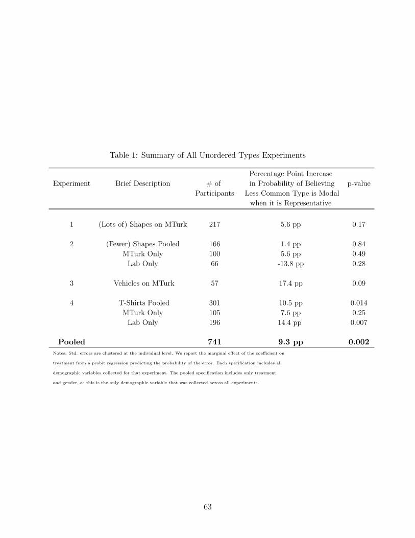
Table 1: Summary of All Unordered Types Experiments

Percentage Point IncreaseExperiment Brief Description # of in Probability of Believing p-value

Participants Less Common Type is Modalwhen it is Representative

1 (Lots of) Shapes on MTurk 217 5.6 pp 0.17

2 (Fewer) Shapes Pooled 166 1.4 pp 0.84MTurk Only 100 5.6 pp 0.49

Lab Only 66 -13.8 pp 0.28

3 Vehicles on MTurk 57 17.4 pp 0.09

4 T-Shirts Pooled 301 10.5 pp 0.014MTurk Only 105 7.6 pp 0.25

Lab Only 196 14.4 pp 0.007

Pooled 741 9.3 pp 0.002Notes: Std. errors are clustered at the individual level. We report the marginal effect of the coefficient on

treatment from a probit regression predicting the probability of the error. Each specification includes all

demographic variables collected for that experiment. The pooled specification includes only treatment

and gender, as this is the only demographic variable that was collected across all experiments.

63

Table 2: Distributions for Ordered Types Experiment 1

Height in Units Counts for Counts for Control Counts for Rep.(Types) Blue Group Red Group Red Group

1 3 3 42 8 9 113 24 23 204 14 14 105 1 1 5

Total Counts 50 50 50Mean Height 3.04 3.02 3.02

E.2 Analysis of All Ordered Types Experiments

We conducted two experiments on ordered types. The final version, using ice cream cones,

was reported in the main text. Here, we report the other experiment and discuss the complete

set of results.

E.2.1 Ordered Types Experiment 1: Rectangles

Our first design for the ordered types experiment used groups of rectangles of varying heights.

We created a group of blue rectangles, each of which were 1-unit wide and 1, 2, 3, 4, or 5 units

tall. In the Control condition, this group was presented next to a group of red rectangles

of the same width with a very similar distribution over heights. In the Rep. condition, the

blue group was presented next to a red group of rectangles with the same width, but with

a distribution over heights that created a representative tall type for the red group. Table

2 displays the distribution, and Figure 9 presents the images, exactly as they appeared to

participants.

In the Control condition, no type is very representative of either group, and the small

difference in the distributions occurs at types close to the mean. In the Rep. condition, on

the other hand, we create a highly representative type for the red group, as there are five

5-unit tall rectangles in the Rep. red group and only one 5-unit tall rectangle in the blue

group. Importantly, across both conditions, the means of the two groups are held constant,

with the blue group always having a mean height of 3.04 units and the red group having a

mean height of 3.02 units. The prediction is that participants will be more likely to guess

64

that the red rectangles are taller on average in the Rep. Condition than in the Control

condition, because of the representative tall type among the Rep. red group.

(a) Control Condition (b) Representativeness Condition

Figure 9: Rectangles Experiment

We chose to arrange the rectangles by height for participants so that it might be easier

to digest and make sense of the groups in a short period of time. We also varied the fill of

the rectangles, with half of each group’s rectangles having a solid fill and half displaying a

checkered fill.47 Our fear was that if only the heights varied by shape, participants might

anticipate that we were particularly interested in their impressions of the heights of the

rectangles. So, we chose to vary the fill as well to create another plausible dimension of

interest.

The first experiment using this rectangles design was conducted on MTurk in November

2014 with 113 participants.48 Participants were randomly-assigned to view either the Con-

trol rectangles or the Rep. rectangles for 15 seconds. Then, they completed simple addition

problems for approximately 3 minutes, computing sums of two-digit numbers. Finally, par-

ticipants were asked questions about the shapes they saw, including which color rectangles

were taller on average, which group of rectangles they would prefer to choose from if they

were going to earn $0.50 per unit height of a randomly-drawn rectangle, and the average

height of each group of rectangles. We also asked about the fill of the rectangles they saw, so47The fill was performed such that approximately half of each type within each group received each fill.

That way, the representativeness patterns we sought to induce in the distributions were preserved withineach fill.

48The HIT was posted once for 100 participants, and 114 completed the experiment via the link toQualtrics. We exclude one participant who self-identified as color blind. The point estimates and p-valuesreported below are unchanged if this participant is included.

65

not all questions would focus on height. Participants received $0.30 and up to an additional

dollar in incentive pay based upon their answers to the questions about the shapes.

The results are consistent with our hypotheses. In the Control condition, 40% of par-

ticipants believed the red group was taller on average, while in the Rep. condition, 60%

of participants believed the red group was taller on average (p=0.03 from two-tailed test of

proportions). When we look at which group of shapes participants preferred to bet on, the

results are weaker but still directionally supportive: 45% of participants in the Control and

58% of participants in the Rep. group prefer to choose from the red shapes when they will

be paid based upon the height of a randomly-drawn rectangle (p=0.16 from two-tailed test

of proportions).

There is no difference in estimated average height of the red shapes across condition (3.28

in the Control versus 3.29 in the Rep. condition, p=0.95). If we look at the estimated average

height of the blue shapes – recall that the blue shapes are identical across condition – we see

that participants in the Rep. condition believe they are slightly smaller on average, though

this difference is not significant (3.30 in the Control versus 3.22 in the Rep. condition, p =

0.59).

We took this design into the laboratory in January 2015 at the Stanford Experimental

Economics Laboratory. There were a few potentially important changes to the protocol in the

laboratory. For one, we had participants complete both an ordered and an unordered types

experiment, back-to-back, in a randomized order. Note that this is the same sample for whom

we reported results for the unordered types Experiment 2 above. Instead of participants

viewing the objects on a computer screen, we passed out envelopes that contained a printed

handout of either the Control or the Rep. shapes. After viewing the handout in the envelope

and completing the math problems, participants were asked to describe the handout they

had seen, in writing, to another participant in the lab. This was incentivized as “advice”,

implemented as described in the previous Stanford laboratory description for unordered types

Experiment 2. We ran four laboratory sessions, with 66 total participants.

The results from the laboratory were inconsistent with our hypotheses. We find that 46%

of participants in the Control condition believed the red shapes were taller on average, while

only 36% of participants in the Rep. condition made this error (p=0.45 from two-tailed

66

test of proportions). When we look at the choices about which group participants preferred

to bet on, the results are even more striking. Nearly 67% of participants in the Control

condition prefer to choose from the red shapes, while only 27% of participants in the Rep.

condition prefer to choose from the red shapes (p=0.001 from two-tailed test of proportions).

Looking at the data on estimated average heights across condition, there are no significant

differences. Directionally, participants estimate both the blue and the red shapes to be taller

on average in the Rep. condition than in the Control condition.

There are a few issues with the rectangles design that we sought to address in later

experiments. First, it may have been tricky for participants to recognize and process heights

of rectangles. We tried to describe the types in terms of “units” of height, but this likely

felt a bit confusing to participants. Therefore, we wanted to move to an ordered space

that had more obviously distinct types. That is why we shifted to using “scoops” of ice

cream, where the difference between 1, 2, 3, 4, or 5 “units” would be more easily recognizable

and familiar. Second, there may have been too many shapes on the page for participants

to make sense of in a 15-second viewing period. Looking at the advice participants wrote

in the laboratory sessions is very informative. Many participants accurately recalled and

described the first row of rectangles (featuring three 1-unit tall blue rectangles and four

1-unit tall red rectangles in the Rep. condition, and three 1-unit red and blue rectangles

in the Control condition), but no advice sheet even attempted to describe the final row. It

may be that with only 15 seconds, participants only have time to focus on part of the page,

and the top of the page may be a likely place to start. This type of behavior would hurt

us substantially: if participants are mostly focused on the top of the page, they will miss

out on the representative tall types we generated. Even worse, in the first row, there are

more short red shapes than short blue shapes in the Rep. condition but not in the Control

condition. This could lead to participants thinking, contrary to our prediction, that the red

group is shorter on average in the Rep. condition. If the first row or two is what participants

mainly recall, it could also explain why so many participants prefer to bet on blue in the

Rep. condition, as they remember there were more of the worst possible payoff shapes among

the red group. We decided to cut down the number of objects in order to give participants

a better chance to view the group as a whole during a short window. And, perhaps more

67

importantly, we altered the distributions so that the group with the representative tall type

would not also have comparatively more of the shortest possible type.

E.2.2 Ordered Types Experiment 2: Ice Cream

In the main text, we reported the results of the ice cream cones experiment. Here, we discuss

those results in more detail. After running the rectangles experiments, we sought to simplify

the protocol as much as possible. We did this by reducing the number of objects, but also by

eliminating the math problems from between the viewing of the objects and the answering

of our questions of interest. This led to the ice cream cone design.

We ran this new simplified ice cream cone design on MTurk in January 2015 with 65

participants.49 When asked which flavor had more scoops on average, 34% of the Control

condition guesses chocolate and 67% of the Rep. condition guesses chocolate (p=0.009). We

ask participants a related question using choices over lotteries. They are told that we are

going to randomly choose one of the ice cream cones they saw, with the participant earning

$0.50 for every scoop the randomly-chosen cone has. They are asked to choose which flavor we

draw from. The proportion that chooses the chocolate lottery grows from 37% in the Control

to 57% in the Rep. condition (p=0.11). Finally, we explore the participants’ estimates of

the average number of scoops on both the chocolate and strawberry cones. In the Control

condition, participants believe the strawberry cones have on average 2.85 scoops and the

chocolate cones have on average 2.82 scoops. In the Rep. condition, participants believe the

strawberry cones have 2.82 scoops on average and the chocolate cones have 2.71 scoops on

average. None of these differences, either across condition or flavor, are significant. Overall,

the fraction of participants who provide greater estimates of the average number of chocolate

scoops than the average number of strawberry scoops is larger in the Rep. conditions than

in the Control conditions (60% versus 40%, p = 0.11 from two-tailed test of proportions).

After running this experiment on MTurk, we sought to bring this design into the labo-

ratory. The first ice cream laboratory protocol used the same ice cream cone images with49We posted the HIT once for 150 participants, with participants randomized in equal proportions into

either this experiment or the vehicles experiment described above. Eighty-four MTurk participants completedthis experiment, but 19 of these individuals had participated in a previous version of this experiment andtherefore are excluded from this analysis. The results reported are unchanged if these participants areincluded.

68

participants directed to answer our questions of interest immediately following the viewing of

the objects. In this way, it was likely quite clear to participants what our goal as researchers

was: to test their recall of the images they saw. While participants on MTurk are often

asked simple attention checks or to report basic objective information (who is this a picture

of, transcribe this audio clip, answer this survey question), participants in the laboratory are

likely less familiar with this type of design. It is possible that they were skeptical or wary of

being tricked – i.e. why am I being asked what seems to be an obvious question?

We had 56 participants complete this experiment at the Ohio State Experimental Eco-

nomics Laboratory in March 2015 before we stopped to evaluate what was going on. The

results from this experiment look similar to the laboratory data from Stanford. In the Con-

trol condition 45% of participants believe the chocolate cones had more scoops on average,

while only 36% of participants in the Rep. condition make this error. The effect goes in the

opposite direction of our prediction, but is not significant (p =0.48 from two-tailed test of

proportions). Similarly, the proportion of people who prefer to bet on the chocolate cones

falls from 48% in the Control to 32% in the Rep. condition (p=0.21). There is no difference

in estimated average number of scoops of either flavor across condition.

Having seen these results, we brainstormed why participants in the Rep. condition in the

lab would be less likely to believe the chocolate cones are taller on average. While an esti-

mated treatment effect of zero would be consistent with noisy data or confused participants,

a directional effect in the wrong way suggests something else at work – something that is

not at work on MTurk, where both the rectangle and the ice cream design produced results

that support our hypotheses. We conjecture that participants in the laboratory are more

skeptical of being tricked, perhaps because they are not usually asked something so simple in

a typical economics experiment. It may also be that our ice cream design was “too good” –

that is, from a quick look at the objects, the chocolate cones quite strikingly appear to have

more scoops on average, that participants are worried that this is actually a trick question.

We do not have direct data on this issue, but we did change the design in an attempt to

address this problem head on.

We used the same distributions of ice cream cones, but added a new, small section on risk

preferences between the viewing of the objects and the questions about the objects. This

69

creates a plausible alternative research question – we could be interested in how viewing a

particular arrangement of ice cream cones impacts a participant’s risk preferences. We paid

participants for this risk preference section, and we framed the questions about the ice cream

cones as more of an attention check than an item of interest. We also added a question to

the very end of the experiment asking participants what they believed the experiment was

trying to test. In this new design, no participant correctly identified our focus on number

of scoops. Our interpretation of the data is that the introduction of this “decoy” encourages

less skepticism on the part of participants, and perhaps helps us more successfully elicit their

quick, gut reactions to the objects, much the way we were able to do on MTurk. This is

speculative, but it does seem consistent with the data we have collected.

We had 101 new participants from the Ohio State Experimental Economics Laboratory

complete the updated ice cream protocol.50 When asked which flavor had more scoops on

average, 51% guess chocolate in the Control and 56% guess chocolate in the Rep. condition

(p=0.61). There are no significant differences in estimates of average scoops across flavor

or condition. The Rep. treatment produces an insignificant decrease in the proportion that

prefer the chocolate lottery (45% to 38%, p=0.47).

A natural question to ask is why results for the choices over lotteries would be weaker

than the results for which flavor had more scoops on average (or which shapes were taller in

the rectangles experiment). While an individual who believes that chocolate cones have more

scoops on average should believe there is also a greater expected value from the chocolate

cone lottery, it does not guarantee that the chocolate cone lottery is the expected utility

maximizing choice: risk preferences may also play a role. Therefore, indicating that chocolate

cones have more scoops on average does not guarantee that a reasonable participant will

also choose the chocolate cone lottery. To shed light on this issue, we asked a different set

of participants from the same laboratory population about their hypothetical preferences

over these lotteries. We presented the three lotteries (chocolate cones, Control strawberry

cones, and Rep. strawberry cones) side-by-side, described as abstract gambles (there was no

mention of ice cream and no visual representation of the lotteries). They were then asked

to rank the attractiveness of these gambles from most to least attractive. In a sample of50Our ex ante target was 100 participants over two days of drop-in sessions.

70

196 participants, 22% prefer the chocolate cones lottery to the lottery induced by the Rep.

strawberry, while 39% prefer that same chocolate cones lottery to the lottery induced by the

Control strawberry cones. This suggests that risk preferences were likely working against us

finding an effect in support of our hypothesis, as this data would predict a 17 percentage

point decrease in the proportion choosing chocolate under the Rep. condition. In light of

this baseline, the fact that we see only a 10 percentage point decrease in the lab and a 20

percentage point increase on MTurk suggests that the presence of diagnostic types is shifting

choices in line with our hypothesis.

E.2.3 Summary of Ordered Types Experiments

Table 3 summarizes the results from the two ordered types experiments. For each experiment,

we run a probit regression predicting the probability that the participant guessed the shorter

group was taller on average from her treatment assignment. We report the marginal effect of

assignment to the Rep. condition (where the tallest possible type is the most representative

type in the shorter group) on the probability of guessing that the shorter group is taller

on average. The last row reports the same coefficient, but from a probit regression that

uses all of the data from the ordered types experiments. We include a dummy for each

particular sample and cluster observations at the individual level. We find a directional

effect consistent with our hypothesis in three of the five samples. When we pool all data, we

estimate that a participant is 11.7 percentage points more likely to believe that the shorter

group is taller on average when it has a representative tall tail. If we include, in addition, all

color blind participants, this estimate is 11.9 percentage points (p=0.022); and, if we include

all observations, including participants who have participated in multiple versions of the

experiment, this estimate is 10.4 percentage points (p=0.040). Note that for ordered types

experiments, there is a significant difference between the laboratory studies and the MTurk

studies. Using only the MTurk example, we estimate that a participant is 25 pp more likely

to guess that the shorter group is taller when it has a representative tall tail (p=0.001); the

estimate for the laboratory sample is directionally negative, -3.5 pp (p=0.51). This difference

in treatment effect across platform is significant (p=0.002).

71

Table 3: Summary of All Ordered Types Experiments

# of Percentage Point IncreaseExperiment Brief Description Participants in Probability of Believing p-value

Shorter Group is Taller onAverage in Rep. Condition

1 Rectangles 179 7.3 pp 0.32Rectangles on MTurk 113 19.1 pp 0.04

Rectangles in Lab 66 -11.0 pp 0.38

2 Ice Cream 223 9.2 pp 0.17No Decoy Ice Cream in Lab 56 -12.0 pp 0.37

Ice Cream on MTurk 65 30.7 pp 0.02Ice Cream with Decoy in Lab 101 3.5 pp 0.73

Pooled 402 11.7 pp 0.03Notes: Std. errors are clustered at the individual level. We report the marginal effect of the coefficient on

treatment from a probit regression predicting the probability of the error. Each specification includes all

demographic variables collected for that experiment. The pooled specification includes only treatment

and gender, as this is the only demographic variable that was collected across all experiments.

72