Publications

9-1997

Stellar Populations and the White Dwarf Mass Function: Stellar Populations and the White Dwarf Mass Function:

Connections To Supernova Ia Luminosities Connections To Supernova Ia Luminosities

Ted von Hippel University of Wisconsin, vonhippt@erau.edu

G. D. Bothum University of Oregon, nuts@moo2.uoregon.edu

R. A. Schommer Cerro Tololo InterAmerican Observatory, rschommer@noao.edu

Follow this and additional works at: https://commons.erau.edu/publication

Part of the Cosmology, Relativity, and Gravity Commons, and the Stars, Interstellar Medium and the

Galaxy Commons

Scholarly Commons Citation Scholarly Commons Citation von Hippel, T., Bothum, G. D., & Schommer, R. A. (1997). Stellar Populations and the White Dwarf Mass Function: Connections To Supernova Ia Luminosities. The Astrophysical Journal, 114(3). https://doi.org/10.1086/118546

This Article is brought to you for free and open access by Scholarly Commons. It has been accepted for inclusion in Publications by an authorized administrator of Scholarly Commons. For more information, please contact commons@erau.edu.

Stellar Populations and the White Dwarf Mass Function:

Connections To Supernova Ia Luminosities

Ted von HippelDept. of Astronomy, University of Wisconsin, Madison WI 53706

email: ted@noao.edu

G. D. BothunDept. of Physics, University of Oregon, Eugene OR, 97403

email: nuts@moo2.uoregon.edu

and

R. A. SchommerCerro Tololo InterAmerican Observatory, La Serena, Chile

email: rschommer@noao.edu

ABSTRACT

We discuss the luminosity function of SNe Ia under the assumption that

recent evidence for dispersion in this standard candle is related to variations

in the white dwarf mass function (WDMF) in the host galaxies. We develop

a simple parameterization of the WDMF as a function of age of a stellar

population and apply this to galaxies of different morphological types. We

show that this simplified model is consistent with the observed WDMF of

Bergeron et al. (1992) for the solar neighborhood. Our simple models predict

that WDMF variations can produce a range of more than 1.m8 in MB(SN Ia),

which is comparable to the observed value using the data of Phillips (1993) and

van den Bergh (1996). We also predict a galaxy type dependence of MB(SN Ia)

under standard assumptions of the star formation history in these galaxies and

show that MB(SN Ia) can evolve with redshift. In principle both evolutionary

and galaxy type corrections should be applied to recover the intrinsic range of

MB(SN Ia) from the observed values. Our current inadequate knowledge of the

star formation history of galaxies coupled with poor physical understanding of

the SN Ia mechanism makes the reliable estimation of these corrections both

difficult and controversial. The predictions of our models combined with the

observed galaxy and redshift correlations may have the power to discriminate

between the Chandrasekhar and the sub-Chandrasekhar progenitor scenarios for

SNe Ia.

Subject headings: galaxies: Supernovae; cosmology: distance scale

– 2 –

1. Introduction

It is generally assumed that type Ia supernovae (SNe Ia) are thermonuclear explosions

of degenerate white dwarfs near the Chandrasekhar limit (cf. Wheeler & Harkness 1990),

or perhaps mergers of white dwarfs (WDs) in a binary system (Paczynski 1985). Either

detonation or deflagration models (Arnett 1969; Nomoto et al. 1976) then produce the visible

energy release that characterize the SN light and velocity curves. Detailed models show

considerable differences in these scenarios (Khokhlov et al. 1993), but their large intrinsic

luminosity coupled with the assumed universal physics involved in the Chandrasekhar mass

limit have led to strong statements concerning the use of the magnitude at maximum

(MB(max)) of SNe Ia as distance indicators (Branch & Tammann 1992).

There has been some recent evidence that a moderate to large dispersion exists in

MB(max), however, and perhaps in the intrinsic color of these objects at maximum. This

evidence has been revealed by the extensive efforts of several groups to obtain high quality

and frequently sampled observations of a large number of SNe. In particular, Phillips (1993)

has summarized high quality SN Ia measurements in nearby galaxies, with the result that

the intrinsic dispersion in MB(max) appears to be ∼ 0.m8, and correlated with the decay

time of the light curve. Furthermore, the underluminous nature of SN1991bg (Filippenko

et al. 1992; Leibundgut et al. 1993) is striking. This apparent dispersion in MB(max) has

led to some discussion of different models of the origin of SN Ia explosions. Unfortunately,

current measurements are insufficient to discriminate in detail between various explosion

models (detonation versus deflagration, etc.) or origin scenarios (see Wheeler & Harkness

1990; Iben & Tutukov 1991; Khokhlov et al. 1993). Woosley & Weaver (1994) and Livne &

Arnett (1995), among others, have discussed explosions of sub-Chandrasekhar limit WDs.

Pinto & Eastman (1997) examine the physics of SN Ia light curves in detail and use an

analytic model to study the sensitivity of the resultant light curves to various properties

of supernova explosions. They find that a variation in total mass can lead to a sequence

of light curves that reproduces the luminosity – decline rate relation. Other possible

parameters (explosion energy, 56Ni mass, and opacity) lead to relations between luminosity

and light curve shape that are opposite to the observed behavior. They conclude that the

total mass of the explosion is a natural and simple explanation of the observations.

If a wider range of masses could be contributing to SN Ia explosions, then the possibility

arises that different stellar populations would produce different origin functions (see also

Kenyon et al. 1993). Moreover, since stellar populations do evolve, SN Ia luminosities may

depend on the particular form of the WDMF which should evolve with redshift. In principle,

these dependencies can produce biases and selection effects in surveys for distant SNe which

become important to evaluate and remove. These include the standard Malmquist bias

– 3 –

concerns, as well as concerns about galaxy type and position dependencies in the detected

SN samples.1 These concerns are standard ones with any extragalactic sample, although

they have not been extensively investigated in the SN studies to date, partly due to the

small sample size (see Ruiz-Lapuente et al. 1995).

At issue here is whether the progenitors of SNe Ia have a significant range in mass,

that in turn produces a range in SN Ia luminosities, or if SNe Ia principally come fron

Chandrasekhar mass white dwarfs. In this paper, we focus attention on the first possibility

and produce a series of models which produce different white dwarf mass functions

(WDMFs) for differing star formation histories. These models have predictive power for

both the range in SN Ia luminosities as well as the mean SN Ia luminosity for a given mean

stellar population age.

However, regardless of the physics that produces SNe Ia, it is now well-established that

empirical corrections to their luminosity based on the form of the light curve (e.g., Riess et

al. 1995,1996; Hamuy et al. 1995, 1996b) produces a Hubble diagram which is linear out to

z = 0.1 with a scatter of ≤ 0m.15. To first order, this argues that the intrinsic range of SN

Ia luminosities is irrelevant as the multi-color light curve (MLCS) and/or luminosity-decline

correlations empirically correct for this range. In fact, these empirical corrections may be so

good that systematic differences between galactic stellar populations may now be revealed.

There is already some observational evidence bearing on this (Hamuy et al. 1996) and so

the principle task of our modelling procedure is to demonstrate how systematic differences

in galactic stellar populations directly lead to systematic galaxy-galaxy differences in SN

Ia luminosities; thus the observed galaxy correlations may have the power to discriminate

between different progenitor models.

In fact, we will demonstrate that our model predicts evolutionary corrections to SN Ia

luminosities that, at z = 0.5, are an important percentage of the total cosmological signal

differential between qo = 0 and qo = 0.5. In light of the concerted efforts being made in the

detection of SNe Ia at redshifts ≥ 0.3 (Perlmutter et al. 1995) and the expectation that

fundamental cosmological parameters can be determined it seems especially important to

understand, in as much detail as possible, the dependence of mean SN Ia luminosity on the

underlying stellar population.

The thrust of this paper evaluates the WDMF and its variation as a function of stellar

population and evolutionary state, under the assumption that the dispersion of MB(SN

1For example, a radial gradient in luminosities of SNe in galaxies could easily exist because of abundance

and age gradients, and combined with the reddening distribution, systematic luminosity differences for SNe

in the outer regions of spiral or irregular galaxies might dominate the observed samples.

– 4 –

Ia) is correlated with the mass of the WD progenitor. In particular we focus on one issue:

how does the WDMF depend on its parent stellar population (Section 2)? We then apply

a simple parameterization of that dependence to two cases of interest: SNe Ia arising

in different galaxy types (populations with different star formation histories), and the

dependence of progenitor mass on cosmological look back time (Section 3). We evaluate

these effects on the determination of qo from z ≥ 0.3 SN Ia detections. Our concern is in

the scatter in the candle, and the zero point of the flux scale is irrelevant for this discussion

(but relevant for Ho).

2. A Simple Parameterization of the White Dwarf Mass Function

We consider the luminosity distribution of SNe Ia to be a separable function, Λ, which

can be written as

Λ = G(m) Nwd L(mwd), (1)

where G(m) is a source function, i.e. a restriction beyond the stellar population inputs

on the mass range of WDs which can become SNe Ia and which would include various

pathways (binary formation, etc.), Nwd is the number distribution given by the WDMF,

and L(mwd) is the conversion from WD mass to luminosity (essentially the Ni mass core

of the exploding WD). For this paper we will assume that G(m) = 1 (i.e., no additional

restrictions beyond those which we model); for the Chandrasekhar mass ignition model,

this function would be a delta function at 1.4M⊙.

We build a simple model of the WD mass distribution as a function of population

age based on prescriptions for the WD initial mass – final mass relation, theoretical stellar

lifetimes, and a star formation rate (SFR) parameterization. We assume that the rate of

formation of stars of a given mass at a given time can be characterized by a separable initial

mass function (IMF) and SFR, as

R(m, t) = Φ(m) (A/ts) e−t/td , (2)

where m is mass in solar units, A is a dimensionless normalization, ts is the dimensional

time unit, td is the decay time of the SFR, and Φ(m) is the IMF of the form

Φ(m) = No mα. (3)

– 5 –

The number of stars which will leave the main sequence to become WDs in a given

mass interval, dm, and in a given time interval, dt, is

dNevol(m, t) = Θ(t− τ(m)) R(t− τ(m)) dmdt, (4)

where τ(m) is the timescale of evolution for a star of mass m, and Θ is a step function

equal to 1 for t ≥ τ(m) and 0 otherwise, and which allows the two cases of t < τ(m) and

t ≥ τ(m) to be compactly written. To determine the number of stars which have evolved

into WDs by a given time, t, the above equation is integrated over t to yield

Nevol(m, t) = Θ(t− τ(m))∫ t

τ(m)dtΦ(m) (A/ts) e

−(t−τ(m))/td dm. (5)

Letting t′ = t− τ(m), then

Nevol(m, t) = Θ(t− τ(m)) Φ(m)dm∫ t−τ(m)

0dt′(A/ts) e

−t′/td (6)

= Θ(t− τ(m)) Φ(m)dm A (td/ts) [1− e−(t−τ(m))/td ]. (7)

To convert Nevol(m, t) to Nwd(m, t) requires an initial mass – final mass relation, which

we achieve from a quadratic parameterization of empirical relation “A” of Weidemann &

Koester (1983):

Mwd = 0.48− 0.016 m+ 0.016 m2, (8)

where m is the initial main sequence mass of a star as used above, and Mwd is the mass

of the resulting WD. This agrees with observations, which are very limited, and gives a

1.376M⊙ WD for m = 8M⊙, which we assume to be the highest mass star that produces a

WD remnant. Clearly, all results we obtain subsequently stem from this parameterization,

and so, to the extent that it can be justified by the observations, we have a reasonably firm

foundation.

We also require τ(m), the pre-WD evolutionary timescales as a function of mass, which

we achieve from a re-parameterization of the equations given in Eggleton et al. (1989). We

simplify their parameterization as we require only lifetimes for stars with masses from 1 to

8M⊙, whereas their equations are valid for 1 to 80M⊙. Additionally, we renormalize their

stellar lifetimes so that a 1M⊙ star has a main sequence lifetime of 1010 years. Following

– 6 –

Eggleton et al. (1989) we also take the post main sequence lifetime to be 15% of the main

sequence lifetime. The resulting parameterization is then

τ(m) = to m−2.8, (9)

with to = 1.15× 1010 years, for m = 1 – 8M⊙. For an 8M⊙ star, the timescale of evolution

is 34 Myrs.

To use the above equations we set A = 1 (arbitrary normalization) and ts = 1 Gyr (i.e.,

all time units in Gyrs). We then choose various SFR models with td = 1, 3, 5, 10, and 100

Gyrs to simulate the range from single age ellipticals to constant star formation spirals. We

explore the range α = 0 to −3 (α = −2.35 is the Salpeter value) for the slope of the IMF

and then calculate Nevol over the range of time until t = 12 Gyrs. Finally, we transform

Nevol to Nwd via the initial mass – final mass relation.

Figure 1 shows the resultant WDMF for different values of the mass function slope

(α = −3,−2,−1, 0) in each panel, for two different SFR decay times (1 Gyr, essentially a

burst; and 100 Gyrs, almost constant SF), and for 6 different ages (0.5, 1, 2, 4, 8, and 12

Gyrs) since the onset of SF.

One immediate test of these models is a comparison with the solar neighborhood WD

mass function. Figure 2 shows the observed mass function of Bergeron et al. (1992). As

they note, this magnitude-limited survey selects against the fainter, low radius (high mass)

WDs. Additional selection may also be caused by the quicker cooling of higher mass WDs,

and possible scale height inflation that would preferentially select against all stars of higher

mass than the current turn-off mass of the disk population. Plotted on this distribution is

our 10 Gyr, steady SFR, α = −2.35, model with an arbitrary normalization. The agreement

is satisfactory after noting that Bergeron et al. (1992) interpret the lowest mass WDs (first

several bins) as likely results of binary evolution. On this basis, we believe that our models

produce WDMFs that are astrophysically reasonable.

3. Luminosity Functions: Predictions, Samples, and Biases

Woosley & Weaver (1994) explored the details of 0.6 – 0.9M⊙ WDs accreting from

a companion post main sequence star. They found a number of scenarios where 0.1 to

0.2M⊙ of material (He) could be accreted before a thermal runaway in the surface layers

occurred. Since these thermal runaways propagate more rapidly around the surface of the

WD than the resulting shock wave propagates into the interior of the WD, the shock wave

– 7 –

is focused in the deep interior, often resulting in a detonation. We use their models as

the basis of our parameterization of the amount of light given off by the supernova (based

on 56Ni production) as a function of mass of the accreting white dwarf. The Woosley &

Weaver models are meant to explore a range of accretion rates and metallicities, and we

parameterize their results as model A, which has a mass accretion rate of 2.5 × 10−8M⊙

yr−1, and model B, which has a mass accretion rate of 3.5× 10−8M⊙ yr−1. Model A creates

SN Ia type explosions for a pre-accretion mass as low as 0.6M⊙, whereas Model B creates

SNe Ia for masses as low as 0.7M⊙. The upper mass limit of their pre-accretion WDs is

0.9M⊙, but we will assume that this relation can be extrapolated up to 1.1M⊙, which is

a likely upper limit to C-O WDs (Iben & Webbink 1989; but see Kippenhahn & Weigert

1990). Our extrapolation and the unknown upper limit is overly simplistic, but is sufficient

for our purposes. Our parameterizations of these two models are then

La(mwd) ∼ mnia (mwd) = −1.2 + 2.4 mwd for mwd ≥ 0.6 and (10)

Lb(mwd) ∼ mnib (mwd) = −1.3 + 2.3 mwd for mwd ≥ 0.7, (11)

where 56Ni masses in excess of 1.376M⊙ are set to 1.376M⊙. This adjustment only affects

WDs in the incremental mass range 1.07 – 1.10M⊙, and only for model A.

The resultant luminosity functions, Λ, from the product of N(m) and L(mwd), are

shown in Figure 3 for several combinations of age, α, and SFR parameterizations. The Λ

functions are very flat, as expected from the nature of the almost power law mass functions

and the simple linear relation between the Ni mass and the WD progenitor mass. These

luminosity functions are strongly non-gaussian, which is likely to be the result in general if

the wide mass range assumption we have made (essentially the Woosley & Weaver models)

are not given any features by the source function, G(m).

Ideally we would now like to rigorously compare Figure 3 with the observed SN Ia

luminosity function. However, it is our contention that the observed LF is poorly known.

Essentially all extant surveys have to be corrected for completeness. These incompleteness

corrections depend on the assumed intrinsic form for Λ2. As such these corrections usually

have the flavor of self-fulfilling prophecies: the derived “σ” will depend on the assumed

dispersion. Since the number of well-measured SNe Ia occurring in host galaxies with well

2So Λobs = S(Λ), where S is a selection function which depends on the magnitude limit and other

properties of the survey.

– 8 –

measured distances is quite low (e.g., the 9 objects in Phillips 1993), neither the intrinsic

LF nor a reliable estimate of the mean MB(SN Ia) can be made from extant data.

As a result of data paucity, the construction of the proper SN Ia LF is currently

an ambiguous and contentious issue which remains unresolved. Figure 4a shows the B

luminosity function for 29 SNe Ia from the Calan/Tololo survey (Hamuy et al. 1995, 1996a),

plus the 9 objects from Phillips (1993). One of our referees argued that the 9 SNe from

Phillips (1993) “over represents” peculiar SNe Ia. We feel this reasoning was circular since

the criteria for inclusion in the Phillips sample is only that a good distance to the galaxy

has been derived (from surface brightness fluctuations or Tully-Fisher measurements).

How could selection based on the existence of an independent distance estimate cause an

over representation of anomalous SNe Ia? In fact, the Phillips criteria is exactly what

should be used in the construction of a representative LF as long as no identifiable bias

exists in the distance determinations to these 9 galaxies. We also choose the Calan/Tololo

sample because it is the largest collection of SNe Ia with homogeneous (although still not

quantified) selection criteria. Figure 4a presents the observed LF, uncorrected for any

probable selection effects. The Phillips (1993) sample of nearby SNe Ia in galaxies has

unknown selection effects, while the Calan/Tololo sample of southern SNe has some galaxy

type dependencies with distance that are still being explored. For this sample, absolute

magnitudes of SNe Ia are assigned using redshift as the distance indicator. The most

significant aspect of Figure 4a is not its shape or mean value but rather the total luminosity

range that is exhibited. The very faint object evident in this figure is SN1991bg, a very red

SN that has been universally tagged as being an anomalous SN.

Figure 4b shows the SN Ia LF for all the SNe from Vaughan et al. (1995) (hereinafter

VBMP) with data obtained after 1970 (30 SNe). If we exclude from the first sample

SN1991bg, the two distributions are essentially identical. For the 30 objects in Figure

4b, the mean B-magnitude is −18.50 ± 0.49 while the mean B-magnitude for the 37

objects in Figure 4a is −18.50 ± 0.4. These dispersions are relatively large, and obviously

uncorrected SNe Ia would not appear to be a premier distance indicator. VBMP claim to

be able to lower this dispersion by identifying and removing SNe with deviant red or blue

color. Since the intrinsic spectral energy distribution of SNe Ia is not yet well known from

theory, a color-based rejection criteria is at best risky. If we examine the 20 objects in

the VBMP sample that were discovered after 1980 and reject SN1991bg and SN1986G (as

obvious deviants), the mean magnitude is −18.40 ± 0.46 (a change of −0.m1 in the mean

is significant in the cosmological context). VBMP reject 3 more objects from this sample,

including the very well studied object SN1989B. VBMP specify the observed color (B−V =

0.30) of SN1989B as being anomalous but Wells et al. (1994) attribute its color to a large

reddening, specifically E(B−V) = 0.37. Removing this single object from the 18 most recent

– 9 –

SNe in the VBMP sample lowers the dispersion from 0.46 to 0.34 mag! Yet if reddening

is the reason for the anomalous color, then obviously the absolute magnitude of SN1989B

is substantially brighter than the value listed in VBMP. After trimming of the anomalous

objects in Figure 4b, VBMP find a distribution with a mean magnitude of −18.54± 0.35.

This mean is very similar to the values we derive for Figure 4a.

We contend that the SN Ia LF is simply not yet well-determined due to limited

sample sizes and survey volumes, and the difficulty of determining direct and independent

distances to many of the host galaxies. While we may have a reasonable estimate for

the maximum brightness of SNe Ia, we do not know the entire LF. Furthermore, the SN

Ia LF of VBMP is not representative of the whole distribution of SN Ia luminosities but

rather of VBMP’s selected sub-sample in which they have chosen to ignore or reject a

fair percentage of the faintest SNe. Are these rejected objects not, therefore, SNe Ia?

Without an adequate explanation of the mechanism that causes the rejected objects to be

anomalously underluminous, it seems premature to a priori exclude them when specifying

the intrinsic range of SN Ia luminosities and then claim that the sample of distant SNe Ia

is identical to the selected sub-sample.

For example, we know that the Calan/Tololo sample has obvious selection effects; SNe

Ia fainter than −18.0 will not be found in at least half the surveyed volume, since they

fall below the apparent magnitude cutoff of the survey. Some of these selection effects are

discussed in Hamuy et al. (1994). While we are not prepared here to analyze completeness

of extant SNe samples, we schematically illustrate our concerns in Figure 5, which shows

the redshift distribution of the Calan/Tololo SN Ia sample. This distribution is extremely

flat, with a median recessional velocity of ∼ 14,000 km s−1, but extending out past 30,000

km s−1. We have included lines in this figure to demonstrate the expected increase in the

sample due to volume effects. The dashed line is a normalization assuming the survey is

complete out to 4,000 km s−1 (which may be representative of the lower luminosity SNe

Ia), while the dotted line assumes it is complete out to 14,000 km s−1 (representative of the

brighter SNe Ia). In either case, we conclude that the sample is severely incomplete through

much of its volume; in the first case it is 98% incomplete at the median redshift of 14,000

km s−1. If the deeper completeness normalization is assumed, the excess of low redshift

SNe are those of fainter absolute magnitude. These comments about incompleteness in the

samples are a reflection of our concerns about the completeness and accuracy of the extant

SN samples which have been used to construct the SN Ia LF.

Our simple model of the range of SN Ia luminosities attempts to explore the systematic

connection between this range and galaxy type. Indeed, it may be very difficult to judge if

the very distant SNe Ia have a broad or narrow distribution of absolute magnitudes, due

– 10 –

to selection effects and cosmological corrections. We are exploring a scenario that makes

certain predictions that can be tested on both local and distant samples.

3.1. Galaxy Population Dependencies

For the purposes of this discussion, we consider that our simple models may be

assigned to galaxy types based on stellar population type. Thus we will assume that we

can characterize elliptical galaxies as single burst models, with the majority of stars formed

12 Gyrs in the past, and with a 1 Gyr exponential decay time. We will also assume a IMF

slope of α = −2 for this single burst model. We will assume an actively star forming galaxy

(SFG) can be characterized by star formation starting approximately 8 Gyrs ago (the

approximate age of the Galactic disk) with effectively continuous star formation (td = 100

Gyrs) and with several IMF slopes. Clearly, these assumptions can be challenged, but they

correctly predict the average UBV color differences between spiral and elliptical galaxies

(see Larson & Tinsley 1978; Bothun 1982). For the cosmological parameters we will assume

Ho = 50 km s−1 Mpc−1 (after all this is a paper on SNe) and qo = 0.5. This universe is less

than 14 Gyrs old.

Although the power law nature of the LFs shown in Figure 3 precludes the calculation

of a reliable mean SN Ia luminosity as a function of galaxy type, we can use these means

to make rough estimates. Figure 6 shows the mean SN Ia luminosities that are obtained by

integrating over the Ni mass distribution as normalized by total number of SN Ia events.

This figure demonstrates that our model LFs do not change shape after ∼ 0.5 Gyrs, which

is the evolutionary timescale of the lowest mass progenitors (3M⊙) which explode as SNe

Ia. We caution, however, that our model does not include the unknown, but possibly large,

time delays inherent in the binary mechanism before mass transfer begins. Thus the large

change in the SN Ia LF shape evident at early times should take place over a greater time

period, making the SN Ia LF more sensitive to stellar population age than this figure

implies. Figure 6 demonstrates that, in the case in which ellipticals and spirals have the

same IMF slope α, the differences in mean SN Ia luminosity are small (≤ 0.04 mag). This

small difference is not surprising as star formation histories with similar α will produce

very similar WDMFs once the mean age is greater than the evolutionary timescale of the

WD progenitors. The difference in mean SN Ia magnitude between an α = −2 elliptical

and an α = 0 spiral is 0m.22. (An even more extreme difference occurs with large lookback

times.) The data from the SN samples support these dependencies on the underlying stellar

population. Hamuy et al. (1996a) find that the brightest SNe occur in late type galaxies

(see their Figure 3) and even more strikingly, that a strong correlation exists between the

– 11 –

decline rate of the SN Ia light curves and the host galaxy morphology (see their Figure

4). Branch et al. (1996) find that SNe Ia that occur in “red” galaxies are 0.3 magnitudes

less luminous than those that occur in “blue” galaxies. While our model calculations are

meant to be illustrative only, they do show that differences in mean stellar population age

and/or slope of the IMF can produce significant differences in mean MB(SN Ia) that are

approximately the same size as the effects seen in existing data samples.

However, variations in mean MB(SN Ia) between galaxy types are not the relevant

quantity with respect to distance measurements. Rather, the total range of MB(SN Ia) is

important, especially when considering the effects of Malmquist bias. In Figure 7 we plot

the initial mass – final mass relation (equation 8) together with nickel mass production. The

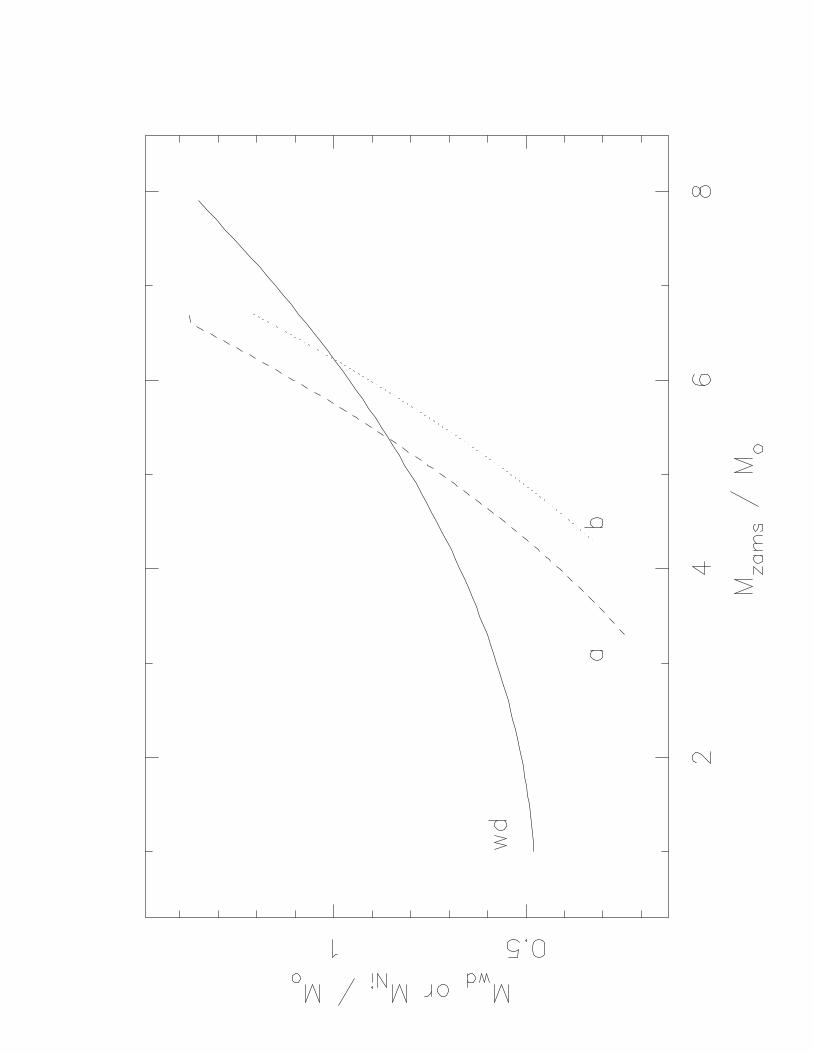
models indicate a range of 4 – 5.5 in Ni mass, which indicates a range in SN Ia luminosities

of up to 1m.8. We terminate our masses at a 1.4M⊙ WD, but if WD mergers at all masses

are a possible channel, then the functions should be continued up to the possible sum of

2.8M⊙, giving a total possible range of 2.6 mags for SN Ia luminosities.

Our predicted range is similar to the observed range shown by Phillips (1993). However,

this comparison is only indirect. Our predicted results are for the SN Ia luminosity range in

a single galaxy for a specific WDMF, whereas in comparing to observations, we are sampling

over a range of galaxy types. Still, the rough agreement between the results based on our

model parameterization and the available observations has an alarming implication: an

order of magnitude range in MB(SN Ia) immediately suggests that Malmquist corrections

are large for any distant extragalactic sample of SNe. We believe the current observations

are effectively sampling this range. That the method of Riess et al. (1996) can lead to

Hubble diagrams with such low dispersions indicates that the light-curve corrections to SN

Ia luminosities are very effective at compressing this intrinsic luminosity range. If these

corrections continue to work well in larger samples, then it becomes clear that the intrinsic

luminosity range of SNe Ia is essentially irrelevant with respect to determining distances.

All that is required is a secure calibration of these light-curve corrected luminosities.

For the simple case in which the Ni mass is proportional to the WD mass (e.g.,

equations 10 and 11), our models predict a spread in SN Ia luminosities of at least 1m.5.

However, invoking variations in WD progenitor mass as the sole cause of the SN Ia

luminosity spread may not be necessary. Various explosion scenarios can easily give 50%

variation in the energy release (Khokhlov et al. 1993; Hoflich et al. 1996). Whether these

models would have a systematic dependency on the WDMF or on the evolutionary state

or metal abundance undoubtedly depends in detail on the nature of the explosion. We

have also ignored any effects of changes in the WDMF on the binary frequency or whatever

progenitors are the SN Ia source G(m) (cf. Kenyon et al. 1993). While the wide binary

– 12 –

source function may be independent to zeroth order of the details of the individual stellar

mass function, the SN Ia source function probably evolved in a more complicated manner

than a simple dependence on mean WD mass. Hence, several physical effects can cause the

SN Ia LF to depart significantly from a delta function.

3.2. Cosmology and Evolutionary Corrections

The redshift – magnitude relation in standard form yields the equation

m = M + 25− 5 log Ho + 5 log cz + 1.086 (1− qo) z + .... (12)

At z= 0.5, for Ho = 50 km s−1 Mpc−1, the difference between qo of 0.0 and 0.5 (empty

versus critical mass models) is 0.m27 (assuming a zero cosmological constant). With

photometric accuracies of ∼ 0.m1 per SN event, statistics of a sample of 10 well-measured

objects would permit an ∼ 8σ discrimination between empty and critical models. Clearly,

however, systematic errors or biases at the 10% level become very significant and lead to an

effective qo measurement.3

For these cosmological parameters the look-back time at z = 0.5 is 3.75 Gyrs.

Inspecting our models we see little change in our E galaxy sources. However, the actively

SFG shows significant evolutionary effects in the sense that the WDMF is populated toward

the more massive objects in the past, and thus the Λ function produces brighter SNe. The

WDMF also depends sensitively on the assumed age parameter for the SFG; if the galaxies

are assumed to initiate star formation 8 Gyrs ago, at z = 0.5 the mean luminosity can be

as large as 0m.31 brighter for the α = 0 case.4

The nature of the general galaxy population at z = 0.5 is still poorly determined. At

a minimum, however, we expect the fraction of young or starbursting galaxies in some

random field to be significantly higher than is observed at the present epoch. The SN Ia

rate at some epoch, z, is a function of the total number of young stars that exist at that

epoch since massive white dwarfs are produced by short-lived stars. Hence, a single, massive

3We would measure qeffo = qo − (dL/dt)/L/Ho, in the case of luminosity evolution, for example.

4We ignore here the K-correction issue, which can be complicated at the few percent level for complex

spectral types such as SNe. For example, different K-corrections are probably necessary at different epochs

for a given supernova event, because of the significant evolution of the spectral energy distribution. Clearly,

shifting the observed bandpass with redshift is an important consideration (cf. Hamuy et al. 1993; Kim et

al. 1996).

– 13 –

starbursting galaxy could completely dominate the rate. Additionally, early star formation

may be characterized by a far different IMF slope than we observe today. This would be

particularly troublesome as the SN Ia LF changes dramatically with IMF slope (see Figure

6). For our purposes, we pose one specific question: how much of a star formation burst

is required to create a significant number of SNe Ia from the burst population relative

to a single-age 5 – 8 Gyr (elliptical) galaxy? SNe that occur in ellipticals (or the old

population in a spiral which we assume is negligible at these redshifts) can be thought

of as being the background SN population against which SNe occurring in star bursting

galaxies are detected. The relative contribution of the SF and background populations can

be parameterized as

No. burst SNe

No. background SNe=

nburst exp(−t/to)

nback exp(−t/to)=

nburst exp(−1 or − 0.5)

nback exp(−8 or − 5)(13)

For population age, t = 5 Gyrs,

(SNburst/SNback) = (nburst/nback) (55− 90) (14)

and for population age, t = 8 Gyrs,

(SNburst/SNback) = (nburst/nback) (1100− 1800). (15)

Table 1 provides the percentage of SNe resulting from a burst as a function of the

percentage of mass in the burst population relative to underlying stellar population. Again,

the values in this table come from considering one single age elliptical with one starbursting

spiral. Column 1 lists the percentage of total SNe that come from the starbursting spiral,

while columns 2 and 3 list the starbursting mass fraction for the t = 5 and 8 Gyrs cases.

For the case of low burst strength (e.g., ≤ 2%), we find the expected result that since

the field contains two galaxies, 50% of the SNe come from one of the two galaxies. However,

for a star formation burst of 10 – 20%, 90% of the SNe will come from that one starburst

galaxy. The situation is even more extreme if we consider a true starburst galaxy (burst

strength ≥ 100%) in which case 99% of the SNe come from that one galaxy. These results

indicate that if a field at z = 0.5 contained 90% ellipticals and 10% starburst spirals with

burst amplitudes of 10 – 20%, then 50% of the total SNe generated by these galaxies would

come from the minority population. If, however, these galaxies are preferentially dusty,

then extinction effects may reduce the detection of SNe Ia from these hosts. Thus, samples

of distant SNe might be dominated by host galaxies which have young mean ages.

– 14 –

4. Conclusions and Caveats

Overall, our simple model of the dependence of the SN Ia luminosity on the underlying

WDMF allows us to make the following predictions:

1. In the mean, the SNe Ia occurring in spiral galaxies should be more luminous than

those occurring in elliptical galaxies; bright SNe Ia in E galaxies should be very rare. This

effect can be seen in the data compilations of Phillips (1993) and in the Calan/Tololo survey

(Hamuy et al. 1995, 1996a).

2. A correlation should exist between SN Ia luminosity and the color of the host galaxy

population, with brighter SNe present in bluer galaxies.

3. The SNe in the disks of spiral galaxies should be more luminous in the mean than

those in the bulges. This effect may be hard to observe because of reddening effects. A

reddening independent light curve parameter (such as ∆m15) should correlate with position

in a spiral galaxy, with the broader light curves (smaller ∆m15 values) preferentially in the

disks or outer regions of the spirals.

4. More distant SNe should show slower light curve decay (smaller ∆m15 values) than

the nearby sample because these SNe are preferentially more luminous. This prediction is a

consequence of both starbursting galaxies dominating distant samples and the Malmquist

bias that directly results from the large range in intrinsic SN Ia luminosities.

5. Distant SNe are expected to come predominantly from bright, blue, spiral or

irregular galaxy hosts, most of which are in an elevated state of star formation. The mean

age of these hosts will be younger than the mean age of most z = 0 calibrating galaxies,

making it important that starburst galaxies like NGC 5253 are included in the local

calibrating sample. We have already shown that MB(max) is sensitive to the mean age of

the stellar population. Thus correcting for this mean age effect requires detailed knowledge

of the nature of the stellar populations in distant galaxies. The predicted difference in

MB(max) obtained under modest assumptions about the star formation history of galaxies

is an appreciable fraction of the cosmological signal that distinguishes qo = 0 from qo = 0.5.

6. The form of the LF for SNe Ia should be approximately a power law (see Figure 3),

if we assume the binary formation function introduces no strong features. Larger samples

of low redshift SNe will be needed to determine this function.

7. In general, the form of the WDMF predicts a range of 1.5–2.5m in SN Ia luminosities.

We have argued that current SN Ia samples have effectively sampled this range in luminosity

and that their usefulness as a distance indicator depends critically on the universality of

the light curve correction algorithms (e.g., MLCS) in compressing this luminosity range.

– 15 –

If many of these predictions are borne out, we would contend that such observational

evidence favors the sub-Chandrasekhar mass hypothesis as the main SN Ia progenitor. In

fairness, our results and modelling procedure and its application to the SN Ia distance scale

are subject to a number of caveats and we close this paper by discussing them.

In converting WD masses into SN Ia luminosities we use the recent calculations for

sub-Chandrasekhar explosions by Woosley & Weaver (1994). These models accurately

reproduce the observed correlation between decline rates of the light curves and luminosity,

and are able to produce more 44Ti and 48Cr than other types of models (see discussion in

Livne & Arnett 1995), which is important in matching solar abundances. The 1D treatment

of Woosley & Weaver (1994) yields similar results to the 2D treatment of Livne & Arnett

(1995). We choose the Woosley & Weaver models because they have clear predictive power,

not because we consider these models to be definitive. While models of Chandrasekhar mass

explosions can also yield a range of luminosity (e.g., Hoflich et al. 1995; 1996), based on the

nature and degree of turbulence in the explosion, we contend that, because the dispersion in

SN Ia luminosities is not small and seems to be correlated with galaxy morphology, effects

in addition to explosion physics most likely produce the observed LF. It is not our intention

to delve into SN explosion physics or discuss which SN models in the literature are more

nearly correct. Instead we have argued that a major part of the observed luminosity range

for SNe Ia can result from a dependence of mean SN Ia luminosity upon the mean stellar

population of the host galaxy.

In this case, the mixture of host galaxy types in any SN Ia sample determines the

LF for that sample. Thus, it is not surprising that there is disagreement over the form of

a typical host galaxy in the SN Ia sample at z = 0. Moreover, our models clearly show

the importance of starbursting galaxies in distant samples. The higher SN Ia rate in these

galaxies allows the minority population to dominate the observed frequency. Since these

galaxies have younger mean ages and hence more extended WDMFs, the range of SN Ia

luminosities is larger than that in a z = 0 spiral or elliptical. Indeed, the distribution of

SN Ia host galaxies in the nearby Universe shows some curious properties which makes it

hard to determine if the typical host is a spiral or an elliptical. For instance, the modestly

star forming galaxy M 100 has had four detected SNe since 1901 (one of which is a type

II), whereas the megastar elliptical M 87 has had zero. NGC 5253, a low mass but actively

star forming galaxy, has had two detected SNe Ia in the last 100 years. By comparison, the

Coma cluster, home to ∼ 10, 00 gas poor L* galaxies (e.g., 104 NGC 5253 masses), has not

had a single SN Ia event detected for the last 22 years.

In contrast to this anecdotal evidence, which suggests that spiral hosts dominate over

elliptical hosts, the 30 or so SNe Ia that have been detected in the Calan/Tololo survey

– 16 –

show nearly equal numbers of elliptical and spiral hosts beyond z = 0.033, demonstrating an

anti-Malmquist bias. The dominance of nearby spiral hosts [at redshifts z ≤ 0.033 (Hamuy

et al. 1996a)], may be a result of the avoidance of nearby clusters in the search fields.

However, in the distant half of the sample no a priori selection against clusters existed,

and hence, proportionately more ellipticals should be in that sample, causing some of the

variation. Thus variation in the S/E host ratio could reflect these selection criteria, as well

as the low space density of relatively unreddened starburst spirals in the local universe

(z ≤ 0.1). It is unlikely, however, that similar circumstances would continue to hold at

larger redshifts.

Finally, we comment on the use of light curve corrections to SN Ia luminosities in the

context of our model. Astrophysical measurements, based on either light curve parameters

(Phillips 1993; Riess et al. 1995,1996; Hamuy et al. 1996a) or spectroscopic analysis (Nugent

et al. 1995), appear to correlate well with peak SN luminosity. Hamuy et al. (1996a) show

that high quality light curves exhibit a characteristic shape and luminosity – decay time

relation (Phillips 1993; hereafter the Phillips relation) that produce significantly improved

peak magnitudes and much more accurate relative distances than the use of a single

absolute magnitude calibration (see also Riess et al. 1995,1996). In the model explored

here, the Phillips relation represents a stellar mass sequence. Although we do not attempt

to derive the relation between light curve parameters and mass explicitly, the luminosity –

mass relation is itself linear.

Intrinsic dispersion around the Phillips relation or the MLCS relation of Riess et al.

(1996) would be caused by additional parameters (e.g., metallicity), which may or may not

correlate with the host galaxy stellar population and the WDMF. It is the dispersion around

these relations that become directly relevant to correcting distant samples for Malmquist

bias. Moreover, corrections to SN Ia peak luminosities using z = 0 light curves may not

be strictly applicable to distant SNe in star-bursting galaxies as such galaxies will be rare

(or perhaps non-existent) in the nearby calibrating sample. At the very least, our models

show that knowledge of the WDMF as inferred from the nature of the stellar population

of the host galaxy is critical in order to determine potential systematic differences in

light-curve shape between the distant host galaxy and the calibrating sample. Minimizing

these differences may well validate the approaches of Hamuy et al. (1995, 1996b) and Riess

et al. (1995,1996) that have produced linear Hubble relations out to z = 0.1 with a scatter

of approximately 0m.13 – 0m.17 (Hamuy et al. 1996b, equations 7 – 9) which raise the

expectation that qo can be determined from such data.

We acknowledge helpful discussions with Karl Fisher, Philip Pinto, and Michael

Richmond. We also acknowledge Mark Phillips, Mario Hamuy, and Nick Suntzeff for

– 17 –

inspiring us to investigate the possible connection between SN Ia luminosities and the

underlying stellar population. Finally, we wish to dedicate this paper to Marc Aaronson,

who would have wanted a thorough investigation of the reliability of SNe Ia as standard

candles.

REFERENCES

Arnett, D. 1969, Ap&SS, 5, 180

Bergeron, J., Saffer, R., & Liebert, J. 1992, ApJ, 394, 228

Bothun, G.D. 1982, ApJS, 50, 39

Branch, D., Romanishin, W., & Baron, E. 1996, ApJ, 465, 73

Branch, D., & Tammann, G. 1992, ARA&A, 30, 359

Eggleton, P.P., Fitchett, M.J., & Tout, C.A. 1989, ApJ, 347, 998

Filippenko, A.V., et al. 1992, AJ, 104, 1543

Goobar, A., & Perlmutter, S. 1995, ApJ, 450, 14

Hamuy, M., et al. 1994, AJ, 108, 2226

Hamuy, M., Phillips, M.M., Maza, J., Suntzeff, N.B., Schommer, R.A., & Aviles, R. 1995,

AJ, 109, 1

Hamuy, M., Phillips, M.M., Schommer, R.A., Suntzeff, N.B., Maza, J., & Aviles, R. 1996,

AJ, 112, 2391 (1996a)

Hamuy, M., Phillips, M.M., Suntzeff, N.B., Schommer, R.A., Maza, J., & Aviles, R. 1996,

AJ, 112, 2398 (1996b)

Hamuy, M., Phillips, M.M., Wells, L.A., & Maza, J. 1993, PASP, 105, 787

Hoflich, P., Khokhlov, A.M., & Wheeler, J.C. 1995, ApJ, 444, 831

Hoflich, P., Khokhlov, A.M., Wheeler, J.C., Phillips, M.M., Suntzeff, N.B., & Hamuy, M.

1996, ApJ, 472, L81

Iben, I., & Tutukov, A. 1991, AJ, 370, 615

Iben, I. & Webbink, R.F. 1989, in White Dwarfs, ed. G. Wegner, (Springer-Verlag: Berlin),

477

Kenyon, S.J., Livio, M., Mikolajewska, J., & Tout, C.A. 1993, ApJ, 407, L81

Khokhlov, A., Muller, E., & Hoflich, P. 1993, A&A, 270, 223

– 18 –

Kim, A., Goobar, A., & Perlmutter, S. 1996, PASP, 108, 190

Kippenhahn, R., & Weigert, A. 1990, in Stellar Structure and Evolution, (Springer-Verlag:

Berlin), 340

Larson, R.B., & Tinsley, B.M. 1978, ApJ, 219, 46

Leibundgut, B., et al. 1993, AJ, 105, 301

Livne, E., & Arnett, D. 1995, ApJ, 452, 62

Nomoto, K., Sugimoto, D., & Neo, S. 1976, Ap&SS, 39, L37

Nugent, P., Phillips, M., Baron,E., Branch, D., & Hauschildt, P. 1995, ApJ, 455, L147

Paczynski, B. 1985, in Cataclysmic Variables and Low Mass X-Ray Binaries, eds. D. Q.

Lamb and J. Patterson, (Reidel: Dordrecht), 1

Perlmutter, S., et al. 1997, ApJ, accepted

Perlmutter, S., et al. 1995, ApJ, 440, L41

Phillips, M.M. 1993, ApJ, 413, L105

Pinto, P.A., & Eastman, R.G. 1997, ApJ, submitted

Riess, A.G., Press, W.H., & Kirshner, R.P. 1995, ApJ, 438, L17

Riess, A.G., Press, W.H., & Kirshner, R.P. 1996, ApJ, 473, 88

Ruiz-Lapuente, P., Burkert, A., & Canal, R. 1995, ApJ, 447, L69

Tammann, G.A., & Sandage, A. 1995, ApJ, 452, 16

van den Bergh, S. 1996, ApJ, 472, 431

Vaughan, T.E., Branch, D., Miller, D.L., & Perlmutter, S. 1995, ApJ, 439, 558 (VBMP)

Weidemann, V., & Koester, D. 1983, A&A, 121, 77

Wells, L.A., et al. 1994, AJ, 108, 2233

Wheeler, J.C., & Harkness, R.P. 1990, Rep.Prog.Phys., 53, 1467

Woosley, S.E., & Weaver, T.A. 1994, ApJ, 423, 371

This preprint was prepared with the AAS LATEX macros v4.0.

– 19 –

Fig. 1.— WDMFs for different IMF slopes (panels display exponential SF duration and IMF

slope) and for 6 different ages (0.5, 1, 2, 4, 8, and 12 Gyrs, bottom to top, respectively). a)

WDMF of burst models with 1 Gyr exponentially decaying star formation; b) WDMF of

active star forming galaxies with 100 Gyr exponential star formation.

Fig. 2.— Observed Galactic WDMF (from Bergeron et al. 1992) plotted versus 10 Gyr,

α = −2.35 model for an active star forming galaxy (100 Gyr exponential star formation).

Fig. 3.— The differential SN Ia luminosity functions of the cumulative (time integrated)

stellar population as derived in the text, for the burst models (a, b) and active SFGs (c, d)

for 2 different mass function slopes (α = −2, 0) and 5 different ages (1, 2, 4, 8, and 12 Gyrs,

top to bottom, respectively).

Fig. 4.— a) Histogram of absolute B magnitudes for SNe Ia in the sample of Phillips (1993)

and the Calan/Tololo survey (Hamuy et al. 1996a). The magnitudes of the 9 events from the

Phillips paper have been adjusted to a zero point consistent with the Calan/Tololo sample

calibration. b) Histogram of absolute B magnitudes for the SNe Ia after 1970 from the

sample from Vaughan et al. (1995).

Fig. 5.— The velocity histogram of the Calan/Tololo SN Ia sample. Shown for comparison

are lines showing the volume increase, normalized to the observed SN number at cz = 4,000

km s−1 (dashed) or cz = 14,000 km s−1 (dotted). Under either assumption, the sample is

seriously incomplete (see text).

Fig. 6.— The mean SN Ia luminosity as a function of age, SF history, and IMF slope for

our model A. The luminosity is in terms of equivalent Ni mass. The clustered lines at a

particular IMF slope are for models with different SF histories, with the solid line being the

td = 1 Gyr (burst) model, the dashed line being the td = 10 Gyr model, and the dotted line

being the td = 100 Gyr (steady SF) model.

Fig. 7.— The relevant mass ranges for creating model SNe Ia. The line marked “WD”

shows the initial mass – final mass relation, whereas the other two lines display the Ni mass

produced in the SN Ia explosions for models A and B, as a function of the main sequence

mass of the progenitor.

– 20 –

Table 1: Burst statistics

N from burst nburst/nback at t=5 nburst/nback at t=8

50% 1- 2% ≤ 0.1%

90 10- 16 ≤ 1

99 110-180 6 - 9

-16 -17 -18 -19 -200

5

10

M(B)

N

b) VBMP sample

-16 -17 -18 -19 -200

5

10

N

a) Calan/Tololo sample

0 5 10 15 20 25 300

10

20

30

40

50

60

Velocity (1000 km/s)

Num

ber

Calan-Tololo SNe

Vel. Histogram