Stellar Magnetospheres Stan Owocki Bartol Research Institute University of Delaware Newark, Delaware...
40
Stellar Magnetospheres Stan Owocki Bartol Research Institute University of Delaware Newark, Delaware USA Collaborators (Bartol/UDel) • Rich Townsend • Asif ud-Doula • also: David Cohen, Detlef Groote, Marc Gagné
-
date post
20-Dec-2015 -
Category
Documents
-
view
215 -
download
0
Transcript of Stellar Magnetospheres Stan Owocki Bartol Research Institute University of Delaware Newark, Delaware...
Stellar Magnetospheres
Stan OwockiBartol Research InstituteUniversity of DelawareNewark, Delaware USA
Collaborators (Bartol/UDel)• Rich Townsend• Asif ud-Doula • also: David Cohen, Detlef Groote, Marc Gagné
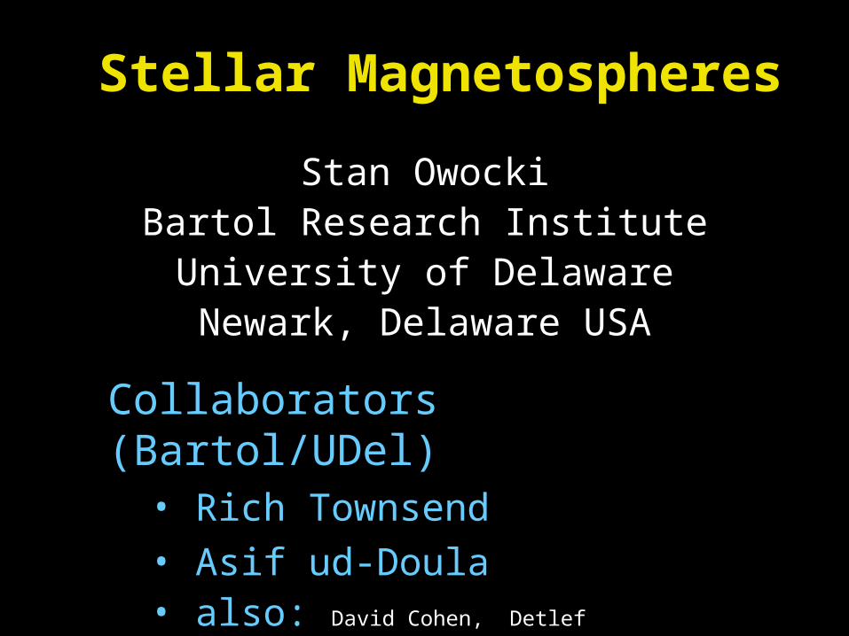
“Magnetosphere”• Space around magnetized planet or astron.body
• coined in late ‘50’s– satellites discovery of Earth’s “radiation belts”– trapped, high-energy plasma
• also detected in other planets with magnetic field– e.g. Jupiter (biggest), Saturn etc. (but not Mars, Venus)
• concept since extended to Sun and other stars– sun has “magnetized corona”– stretched out by solar wind
• but study has some key differences...

Planetary vs. Stellar Magnetospheres
• outside-in compression
• Space physics• local in-situ meas.• plasma parameters• plasma physics models
• inside-out expansion• Astrophysics• global, remote obs.• gas & stellar parameters
• hydro or MHD models
Solar coronal expansion
Interplanetary medium
Solar astrophysics includes both approaches

Earth’s Magnetosphere
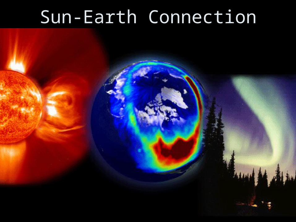
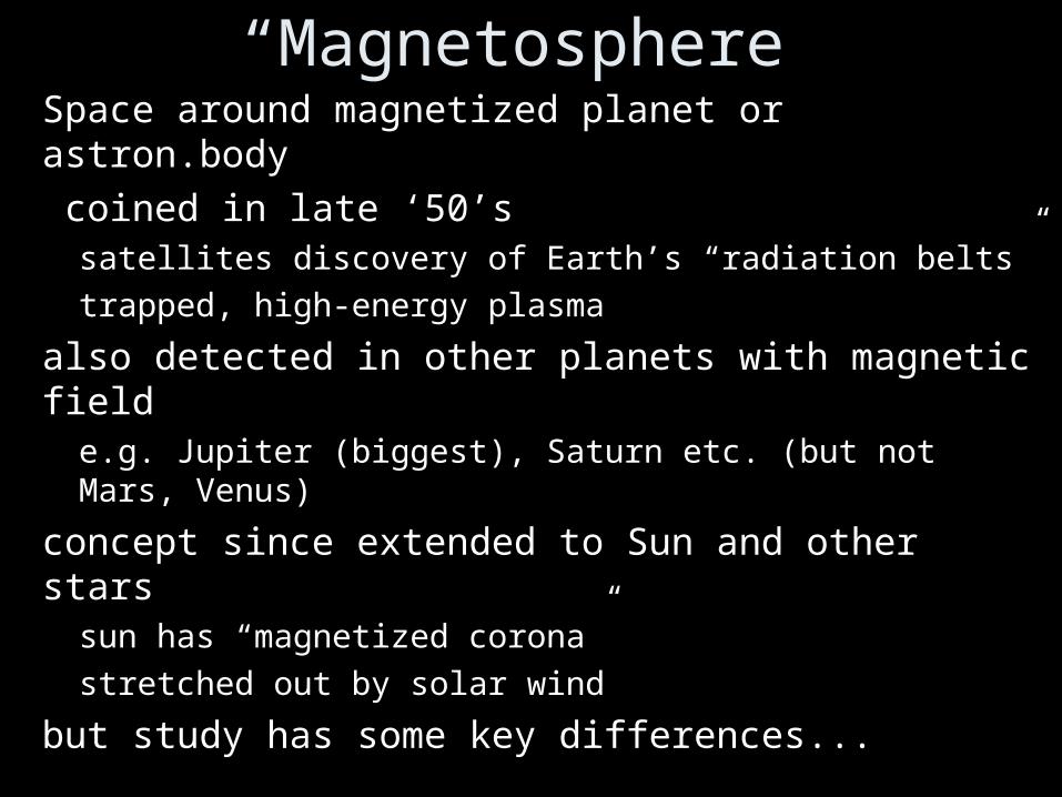
Sun-Earth Connection

Magnetic loops on Solar limb
QuickTime™ and aPhoto decompressor
are needed to see this picture.
Solar Flare
QuickTime™ and aPhoto decompressor
are needed to see this picture.

Sun’s Active “Magnetosphere”

Solar Activity: Coronal Mass Ejections
QuickTime™ and aMPEG-4 Video decompressor
are needed to see this picture.

Processes for Solar Activity
• Convection + Rotation Dynamo– Complex Magnetic Structure– Magnetic Reconnection– Coronal Heating– Solar Wind Expansion + CME

Solar Corona in EUV & X-rays Composite EUV image from EIT/SOHO X-ray Corona from SOHO

Magnetic Effects on Solar Coronal ExpansionCoronal streamers

Corona during Solar Eclipse

Latitudinal variation of solar wind speed
Coronal streamers

Pneuman and Kopp (1971)
MHD model for base dipolewith Bo=1 G
Iterative scheme
MHD Simulation
Fully dynamic, time dependent

MHD model for magnetized plasmas
•ions & electrons coupled in “single fluid”– “effective” collisions =>– Maxwellian distributions
•large scale in length & time– >> Larmour radius, mfp, Debye, skin– >> ion gyration period
•ideal MHD => infinite conductivity

Magnetohydrodynamic (MHD) Equations
DρDt
+ ρ∇⋅v=0
Mass Momentum
mag Induction Divergence free B
€
P = ρa2 = (γ −1)e
De
Dt+γe∇⋅v=H −C
€
ρ DvDt
= −∇p+1
4π∇ × B( ) × B + ρ (gext − ggrav )
€
∂B∂t
=∇ × v × B( )
€
∇• B = 0
Energy Ideal Gas E.O.S.
€
∂e∂t
+∇ ⋅ev = −P∇ ⋅v+ H −C

Maxwell’s equations
Induction
no mag. monopoles
€
∇×E = −1
c
∂B
∂t
€
∇• B = 0€
∇• E = 4πρ e
Coulomb
€
∇×B =4π
cJ +
1
c
∂E
∂tAmpere
€
Ov
c
⎛
⎝ ⎜
⎞
⎠ ⎟2
<<1

Magnetic Induction & Diffusion
€
J =σ (E + v × B /c)
magnetic induction
Combine Maxwell’s eqns. with Ohm’s law:
∂B∂t
= ∇ × v × B( ) +c2
4πσ∇2B
Eliminate E and J to obtain:
magnetic diffusion

Magnetic Reynold’s number
€
Re ≅4πσLv
c 2
∂B∂t
= ∇ × v × B( ) +c2
4πσ∇2B
induction diffusion
€
≅induction
diffusion>>1
€
O1
Re
⎛
⎝ ⎜
⎞
⎠ ⎟<<1“Ideal” MHD
e.g., 1010!
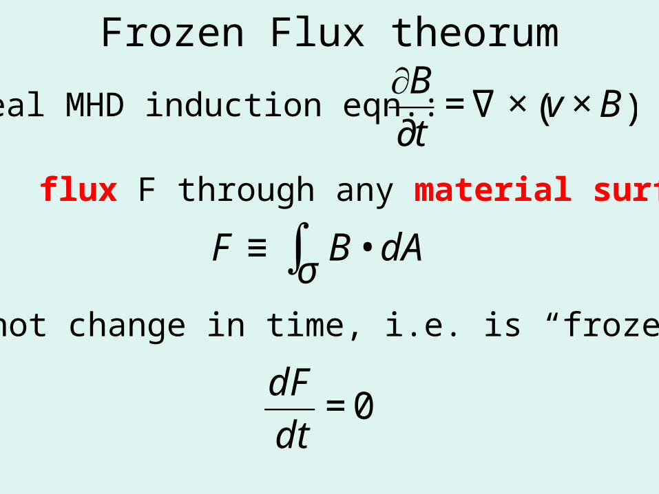
Frozen Flux theorum
€
∂B∂t
=∇ × v × B( )Ideal MHD induction eqn.:
€
F ≡ B • dAσ∫
implies flux F through any material surface
€
dF
dt= 0
does not change in time, i.e. is “frozen”:

Magnetic loops on Solar limb
QuickTime™ and aPhoto decompressor
are needed to see this picture.
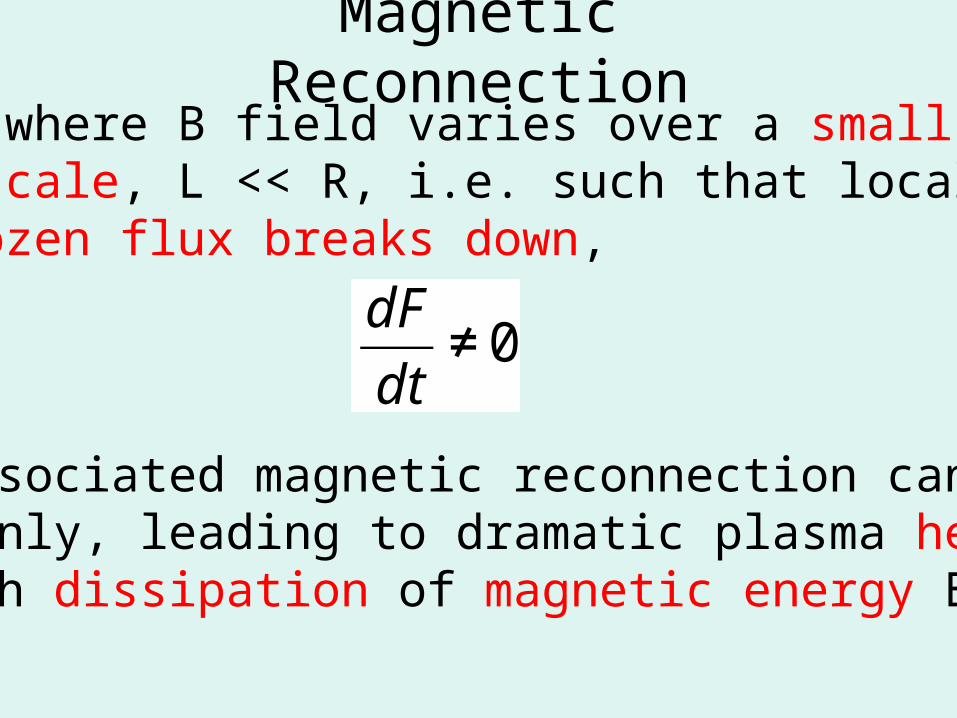
Magnetic Reconnection
If/when/where B field varies over a small enough scale, L << R, i.e. such that local Re~1,then frozen flux breaks down,
€
dF
dt≠ 0
The associated magnetic reconnection can occur suddenly, leading to dramatic plasma heating through dissipation of magnetic energy B2/8.

Solar Flare
QuickTime™ and aPhoto decompressor
are needed to see this picture.

Magnetic Lorentz force:magnetic tension and
pressure
€
fLor =J × B
c
magnetictension
Lorentz force
€
fLor =B • ∇B
4π−∇
B2
8π
⎛
⎝ ⎜
⎞
⎠ ⎟
Use BAC-CAB + no. div. to rewrite:
magnetic pressure
€
=1
4π∇ × B( ) × B

Alfven speed
€
VA ≡B
4πρ
Alfven speed
€
ρVA2
2=B2
8π
Note:
€
=Pmag
€
=Emag
€
a ≡Pgasρ
Compare sound speed
€
Pgas = ρa2
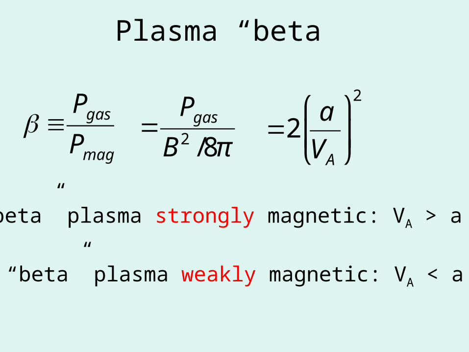
Plasma “beta”
low“beta” plasma strongly magnetic: VA > a
€
=2a
VA
⎛
⎝ ⎜
⎞
⎠ ⎟
2
€
β ≡PgasPmag
€
=Pgas
B2 /8π
high “beta” plasma weakly magnetic: VA < a
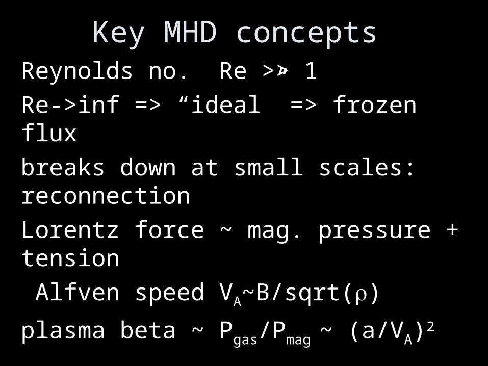
Key MHD concepts •Reynolds no. Re >> 1•Re->inf => “ideal” => frozen flux
•breaks down at small scales: reconnection
•Lorentz force ~ mag. pressure + tension
• Alfven speed VA~B/sqrt(ρ)
•plasma beta ~ Pgas/Pmag ~ (a/VA)2
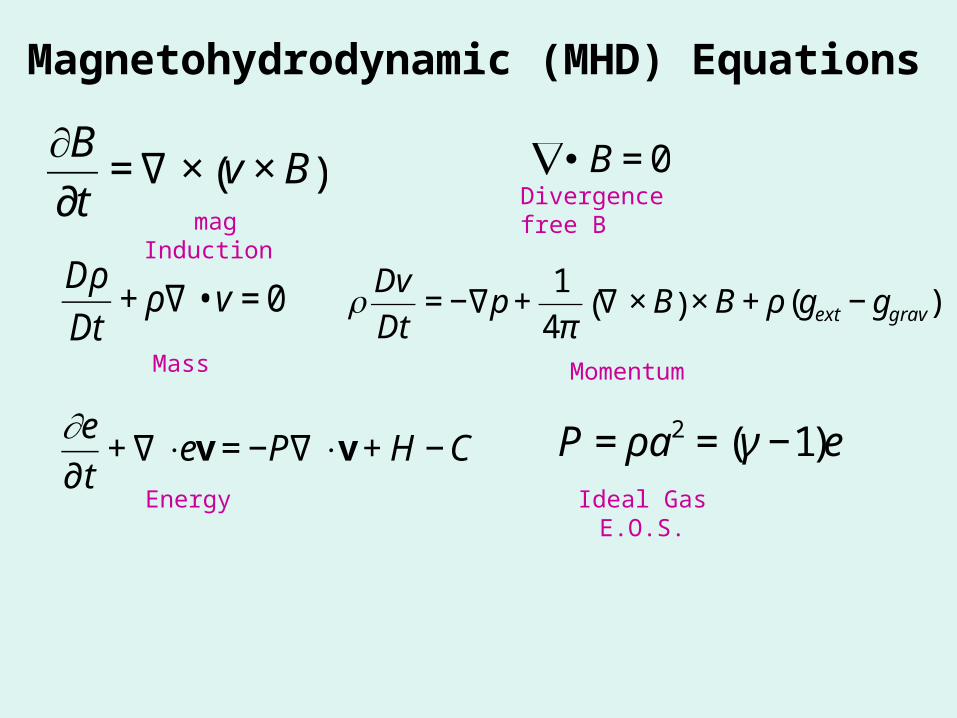
Magnetohydrodynamic (MHD) Equations
€
Dρ
Dt+ ρ∇ • v = 0
Mass Momentum
mag Induction Divergence free B
€
P = ρa2 = (γ −1)e
€
∂e∂t
+∇ ⋅ev = −P∇ ⋅v+ H −C€
ρ DvDt
= −∇p+1
4π∇ × B( ) × B + ρ (gext − ggrav )
€
∂B∂t
=∇ × v × B( )
€
∇• B = 0
Energy Ideal Gas E.O.S.

Apply to solar corona & wind
•Solar corona–high T => high Pgas
–scale height H ~< R–breakdown of hydrostatic equilibrium–pressure-driven solar wind expansion
•How does magnetic field alter this?–closed loops => magnetic confinement–open field => coronal holes –source of high speed solar wind

Hydrostatic Scale Height
€
≈T6
14Scale Height:
€
H
R=a2R
GM €
P = ρa2
€
≡a2
H
€
H
R≈
1
2000 solar photosphere:
€
T6 = 0.006
€
−GM
r2=
1
ρ
dP
dr
Hydrostaticequilibrium:
€
H
R≈
1
7 solar corona:
€
T6 = 2

Failure of hydrostatic equilibrium for hot, isothermal corona
€
0 = −GM
r2−a2
P
dP
dr
hydrostaticequilibrium:
€
P(r)
Po= exp −
R
H1−
R
r
⎛
⎝ ⎜
⎞
⎠ ⎟
⎡
⎣ ⎢
⎤
⎦ ⎥
€
logPTRPISM
⎛
⎝ ⎜
⎞
⎠ ⎟=12observations for
TR vs. ISM:
# decades of pressure decline:
€
logPoP∞
⎛
⎝ ⎜
⎞
⎠ ⎟=R
Hloge ≈
6
T6€
→ exp −R
H
⎡ ⎣ ⎢
⎤ ⎦ ⎥ for r → ∞
Solar corona T6 ~ 2 => must expand!

Spherical Expansion of Isothermal Solar Wind
Momentum and Mass Conservation:
€
vdv
dr= −
GM
r2−a2
ρ
dρ
dr
€
d ρvr2( )
dr= 0
Combine to eliminate density:
€
1-a2
v2
⎛
⎝ ⎜
⎞
⎠ ⎟vdv
dr=
2a2
r−GM
r2
RHS=0 at “critical” radius:
€
rc =GM
2a2
€
v2
a2- ln
v2
a2= 4 ln
r
rc+
4rcr
+CIntegrate for transcendental soln:
€
v rc( ) ≡ a
€
C = −3=> Transonic soln:
€
rc = rs sonic radius

Solution topology for isothermal wind
C=-3

Corona during Solar Eclipse

Kopp-Holzer Non-Radial Expansion

Mach number topology

Latitudinal variation of solar wind speed
Coronal streamers

MHD model for coronal expansion vs. solar dipole
Pneumann & Kopp 1971Iterative solution MHD Simulation

Wind Magnetic Confinement
€
η(r) ≡B2 /8π
ρv 2 /2
Ratio of magnetic to kinetic energy density:
e.g, for dipole field, q=3; η ~ 1/r 4
€
=B2r2
M•
v=B*
2R*2
M•
v∞
(r /R*)2−2q
(1− R* /r)β
η*
for solar wind with Bdipole ~ 1 G: η*~ 40
η* >>1 => strong magnetic confinement of wind