
Steel heat treating: industrial process, mathematical ... · XIII Modelling Week 2019 - Problem 4...
28
XIII Modelling Week 2019 - Problem 4 Steel heat treating: industrial process, mathematical modelling, free software implementation and numerical simulation Bruno Degli Esposti 1 , Claudia Garcia 2 , Jos´ e Miguel Herrera 2 , Jos´ e Ram´ on Obaya 2 , Desy Paone 3 , Edoardo Prezioso 3 1 Universit` a Degli Studi Firenze 2 Universidad Complutense de Madrid 3 Universit` a Degli Studi Di Napoli Federico II Supervised by: Francisco Orteg´ on Gallego Departamento de Matem´aticas Universidad de C´adiz June 2019
Transcript of Steel heat treating: industrial process, mathematical ... · XIII Modelling Week 2019 - Problem 4...

XIII Modelling Week 2019 - Problem 4
Steel heat treating: industrial process,mathematical modelling, free software
implementation and numerical simulation
Bruno Degli Esposti1, Claudia Garcia2, Jose Miguel Herrera2,Jose Ramon Obaya2, Desy Paone3, Edoardo Prezioso3
1Universita Degli Studi Firenze2Universidad Complutense de Madrid
3Universita Degli Studi Di Napoli Federico II
Supervised by:
Francisco Ortegon Gallego
Departamento de MatematicasUniversidad de Cadiz
June 2019

CONTENTS CONTENTS
Contents
1 Introduction 3
2 Introduction to the Modeling Problem 52.1 Introduction to Freefem++ . . . . . . . . . . . . . . . . . . . . . . . . . . 52.2 Building a 2D-mesh . . . . . . . . . . . . . . . . . . . . . . . . . . . . . . . 52.3 Elliptic Equation . . . . . . . . . . . . . . . . . . . . . . . . . . . . . . . . 82.4 Parabolic Equation . . . . . . . . . . . . . . . . . . . . . . . . . . . . . . . 9
3 3D Mesh creation 113.1 Gear construction . . . . . . . . . . . . . . . . . . . . . . . . . . . . . . . . 11
3.1.1 The toothed surfaces . . . . . . . . . . . . . . . . . . . . . . . . . . 113.1.2 The inner and the outer surfaces . . . . . . . . . . . . . . . . . . . 13
3.2 The 3D gear: straight and helicoidal . . . . . . . . . . . . . . . . . . . . . 133.2.1 An optional work: a conic gear . . . . . . . . . . . . . . . . . . . . 143.2.2 Coding 3D mesh with FreeFem++ . . . . . . . . . . . . . . . . . . . 15
4 Heating Problem 164.1 Induction heating simulation . . . . . . . . . . . . . . . . . . . . . . . . . . 164.2 Flame hardening simulation . . . . . . . . . . . . . . . . . . . . . . . . . . 19
5 Cooling problem 21
6 Conclusions 26
7 Future work 27
2

1 INTRODUCTION
1 Introduction
Steel is an alloy of iron and carbon and it is used in industry to manufacture mechanicalpieces that are going to be exposed to high stresses as they are in close contact in order totransmit the desired rotation/translation movement.
In order to avoid these stresses on the piece, a heat treating is made, making they lifetimelonger. The steel heat treating produces a hard boundary layer to prevent abrasion and asoft inner part to reduce fatigue.
It is important to know some physical or mechanical properties of steel in order tounderstand why raw steel is a ductile material and why it can be hardened at critical partschanging its mechanical properties.
Steel can be found in nature in two different crystal lattices, face centered cubic (fcc)and body centered cubic (bcc).
(a) Body Centered Cubic (bcc) (b) Face Centered Cubic (fcc)
As can be observed, the face centered cubic crystal lattice is denser than the bodycentered cubic and, therefore, it is more compact. There are different solid phases in steel:
• Austenite: is a solution of carbon in a face centered cubic iron. The only way to getaustenite is having a carbon concentration lower than 2.11%; if so, only is possible ata high temperature range.
3

1 INTRODUCTION
• Ferrite: nearly pure body centered cubic iron.
• Pearlite: lamellar structure of ferrite and cementite.
• Martensite: tetragonally body centered cubic iron crystal distorted by Carbon atoms.It can only stem from austenite.
The main difference between them is the cooling strategy. If the austenite is coolingdown too fast, martensite is obtained. On the other hand, if the austenite is cooling downslow, perlite is obtained. It can be observed in the following diagram.
4

2 INTRODUCTION TO THE MODELING PROBLEM
2 Introduction to the Modeling Problem
The mathematical description of the steel heating treating is given by a system of nonlinearPDEs in a 2D/3D setting subject to boundary/initial value problems governed by ellipticand parabolic partial differential equations, precisely.It recommended to have meticuloushandling on Lax-Milgram’s theorem to have a uniqueness and existence of the solutionfor the elliptic PDE formulation; Sobolev spaces used to reduce the domain, where willbe applied the boundary conditions; and transform the nonlinear problem into linear andresolve it with the finite element method with the Galerkin-Method. Moreover, implementthe problem with numerical software and can to look at the numerical solution graphicallyin order to compare with the physical solution. We provide you with some free efficientpackages software, namely Freefem++, MEdit and gmsh.
2.1 Introduction to Freefem++
Freefem++ is used for partial differential equation resolution with finite element method.Specifically, it is an integrated software solving PDE of elliptic type. By means someof semidiscretization in time scheme, Freefem++ may also deal with parabolic/ellipticevolution problems.
To solve the problem in question with Freefem++ it is possible follows that scheme:preprocessing (building a mesh in 2D/3D in order to realize the construction the domain toapproximate the gear), find a variational formulation mathematically, and processing (inorder to obtain and visualize the numerical solution).This software can be freely downloadedfrom the Internet (http://www.freefem.org/ff++/index.htm) and it is fully documented.
2.2 Building a 2D-mesh
This section is devoted to the triangulation of domain. The domain considered Ω is acircumference with an inner ellipse Γ, where ∂Ω = ΩD ∪ΩN with ΩD and ΩN Dirichlet andNeumann boundary condition respectively, from the PDEs equation that will be consideredin that section.Freefem++ use the finite element method to build a mesh. We discretizedthe space in order to have finite dimension.The purpose is to divided the domain in trianglesas a graph with nodes and edges and the nodes represent the discretized points of space.
For simplicity, we assume that Ω ⊂ R2 is a polygonal, so that we are able to tile thedomain with a set of triangles ∆k, k=1,....,K defining a triangulation Th. This means thatthe vertices of neighboring triangles coincide and that:
• ∪k∆k = Ω
• ∆l ∩∆m = ∅ for l 6= m
5

2.2 Building a 2D-mesh 2 INTRODUCTION TO THE MODELING PROBLEM
Figure 2: Example of triangular mesh
Surrounding any node is a patch of triangles that each have that node as a vertex(seeFigure 2). If we label the nodes j = 1, ..., n, then for each j, we define a basis function φj
that is nonzero only on that patch φj is a linear function on each triangle, which takes thevalue one at the node point j and zero at all other node points on the mesh.
Moreover, although φj has discontinuities in slope across element boundaries, it issmooth enough that φj ∈ H1(Ω). To make that triangulation with Freefem++ need touse the functions: ”border” (to build up the boundary) and ”buildmesh” (to build a meshwith the contours used in ”border”).
Shown in the following figure:
adding(mesh Th=buildmesh(Gamma1(10)+Gamma2(20)+Gamma3(40)) in the code,it is possible build the triangles, where Gamma1, Gamma2 are the contours of the circum-ference with Dirichlet and Neumann boundary condition respectively, and Gamma3 for theboundary of the ellipse. Numbers (10),(20),(40) represent the number of the points thatwe have considered to discretize the domain.
6

2.2 Building a 2D-mesh 2 INTRODUCTION TO THE MODELING PROBLEM
Moreover, using the function ”plot” we can obtain the numerical solution with Freefem++(see Figure 3). Indeed it returns a graphical solution shown below. It appears a moredense discretization inside the ellipse than outside because in the code shown before wehave considered a different numbers of points to take for Gamma1, Gamma2, Gamma3.
Figure 3: Approximation Numerical Solution with Freefem++ software.
7

2.3 Elliptic Equation 2 INTRODUCTION TO THE MODELING PROBLEM
2.3 Elliptic Equation
The Poisson equation
(1) −∆u = f
is the simplest and the most famous elliptic partial differential equation. The source func-tion f is given on some two- or three-dimensional domain denoted by Ω ⊂ R2 or R3. Asolution u satisfying (1) will also satisfy boundary conditions on the boundary ∂Ω of Ω; forexample:
(2) u = g on ∂ΩD
(3) ∂u∂n
= h on ∂ΩN
where ∂u∂n
denotes the directional derivative in the direction normal to the boundary ∂Ω.
In order to write the elliptic equation in Freefem++ must be manipulated that equationapplying Gauss theorem and integration by part to get the order reduced from second-orderto first-order. The variational formulation will have this shape,
a(u, v) = f(v) ∀v ∈ V
This can be written in matrix form as the linear system of equations:
Au = f
where A is a symmetric matrix and the equation is called Galerkin system.
Numerical form for Freefem++ is shown in (Figure 4), where the chosen functions are:f = 3x+ y, g = x2, h = y3;
Figure 4: Freefem++ Code.
8

2.4 Parabolic Equation 2 INTRODUCTION TO THE MODELING PROBLEM
A possible solution of this problem with the Freefem++ software is represented in(Figure 5). Freefem++ use colors to underline the different level lines during the time.
Figure 5: Numerical Simulation result of elliptic equation.
2.4 Parabolic Equation
Parabolic Equation or Heat Equation
(1) ∂u∂n− k∆u+ a∇u = f in Ω
(2) u = g on ∂ΩD
(3) ∂u∂n
= h on ∂ΩN
u represent the temperature field in Ω subject to the external heat source f. Other im-portant physical models include gravitation, electromagnetism, elasticity and inviscid fluidmechanics. Necessary is the time discretization in order to write the parabolic equationin Freefem++ language and to find a variational formulation.This time discretization inpossible for the Crank-Nicolson Method.
9

2.4 Parabolic Equation 2 INTRODUCTION TO THE MODELING PROBLEM
A code in Freefem++ is written (shown below):
In the numerical simulation obtained from Freefem++ (Figure 6) is clearly visible theheat diffusion with time values t.
On right-side is represented Neumann Condition and on the left-side Dirichlet.The Heatis concentrated more on the second one where there is the red color.
Figure 6: Numerical simulation result of heat equation.
10

3 3D MESH CREATION
3 3D Mesh creation
As it has been shown before, the illustrated method for the 2D mesh construction withFreeFem++ has been straightforward. It will be seen that the method for the 3D meshconstruction results straightforward as well, allowing the construction of complicated fig-ures, as long as the mathematical formulas for the generation of the boundary are provided.For a convenience in the exposure, a brief recap of the 3D mesh characteristics is shown.
A 3D mesh is composed by 3D polygons, but most works use in particular tetrahedra,which are the most simple geometric objects which can be built in 3D. For the creationof the 3D mesh, the mesh of the skin of the object is required. It is important to notethat the skin is made by composing multiple surfaces, such that their sum matches theboundary of a compact and connected 3D set, i.e. it should not present ”holes”, nor jumpdiscontinuities. The construction of the 3D mesh of the surface requires the creation of the2D mesh of a suitable planar geometry, then a mathematical transformation to give shapeand orientation in the 3D world is used. This is discussed for the mesh creation of thehelicoidal gear.
3.1 Gear construction
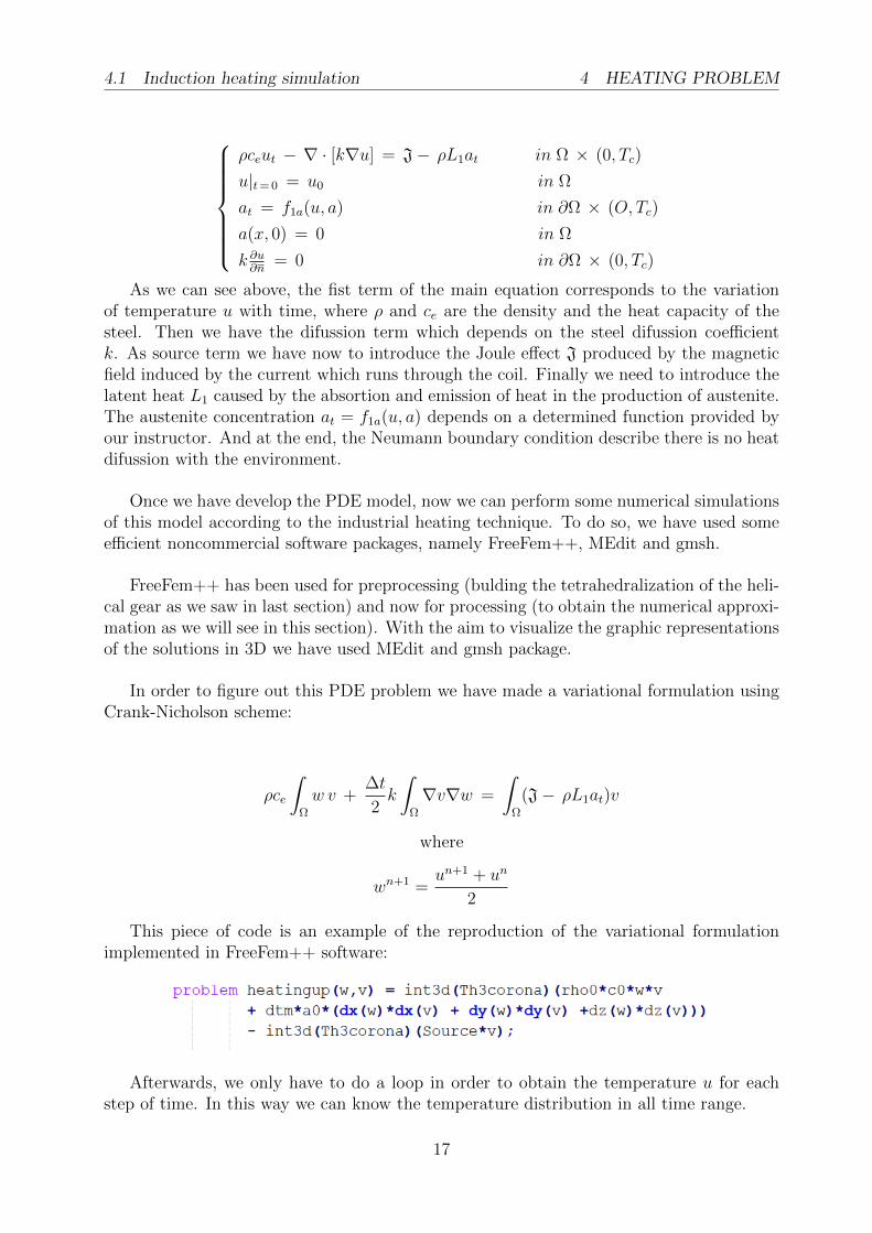
In this project, the most simple model of the gear is constructed by creating four pieces:Su, Sd, Si and So. Both Su and Sd are the toothed annulus and are placed above and belowthe gear, respectively, while Si is the inner cylinder characterizing the ’hole’ and So is thetoothed outside surface.
3.1.1 The toothed surfaces
The construction of Su (or equivalently Sd) is made by an annulus with the external circletransformed to a truncated sinusoidal line. The equation describing its inner circle is thefollowing:
x(t) = γRe cos(t)
y(t) = γRe sin(t)t ∈ [0, 2π] (1)
, with Re the radius of the outer circle, γ the radius portion for the inner circle (which is,the inner radius is γRe ). The outer curve is obtained by the composition of the followingfunctions:
F (t) = cosNT t t ∈ [0, 2π] (2)
, which describes a parametric sinusoidal function with parameter NT (the number ofthe dents of the gear),
RC(t) =
F (t), |F (t)| ≤ C
−C, F (t) ≤ −CC, F (t) ≥ C
(3)
11
3.1 Gear construction 3 3D MESH CREATION
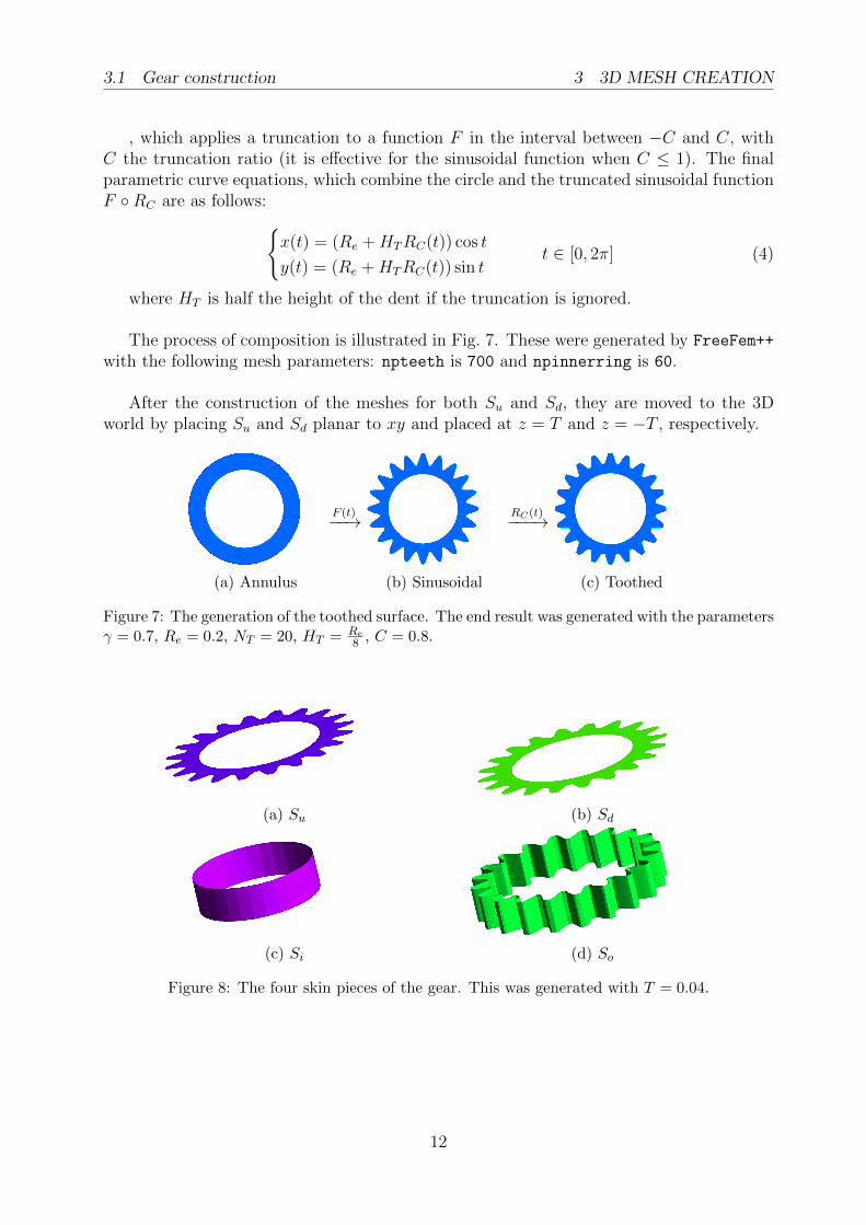
, which applies a truncation to a function F in the interval between −C and C, withC the truncation ratio (it is effective for the sinusoidal function when C ≤ 1). The finalparametric curve equations, which combine the circle and the truncated sinusoidal functionF RC are as follows:
x(t) = (Re +HTRC(t)) cos t
y(t) = (Re +HTRC(t)) sin tt ∈ [0, 2π] (4)
where HT is half the height of the dent if the truncation is ignored.
The process of composition is illustrated in Fig. 7. These were generated by FreeFem++
with the following mesh parameters: npteeth is 700 and npinnerring is 60.
After the construction of the meshes for both Su and Sd, they are moved to the 3Dworld by placing Su and Sd planar to xy and placed at z = T and z = −T , respectively.
(a) Annulus
F (t)−−→
(b) Sinusoidal
RC(t)−−−→
(c) Toothed
Figure 7: The generation of the toothed surface. The end result was generated with the parametersγ = 0.7, Re = 0.2, NT = 20, HT = Re
8 , C = 0.8.
(a) Su (b) Sd
(c) Si (d) So
Figure 8: The four skin pieces of the gear. This was generated with T = 0.04.
12

3.2 The 3D gear: straight and helicoidal 3 3D MESH CREATION
3.1.2 The inner and the outer surfaces
Both Si and So are built from a rectangle D = [0, 2π] × [0, 2T ]. In the 3D world, Si isdefined by the following transformation:
TSi:
[xy
]∈ D −→
γRecos(x)γResin(x)
y
(5)
which defines a cylinder. For surface So, this is the transformation:
TSo :
[xy
]∈ D −→
(Re +HTRC(t)) cosx(Re +HTRC(t)) sinx
y
(6)
3.2 The 3D gear: straight and helicoidal
The four skin pieces of the gear are represented by Fig. 8.
These images were created with the tool Gmsh from the single meshes of the surfaces.The 3D mesh can be created from just the skin of the object by using the software
library TetGen [6]. The result of the final merge and the 3D mesh construction is displayedin Fig. 9.
Figure 9: The straight gear.
The original problem was to solve the heat equation for a helicoidal gear. This isobtained by transforming a straight gear through this mathematical function:
TGhel:
xyz
∈ G −→ cosαz sinαz 0− sinαz cosαz 0
0 0 1
xyz
=
x cosαz + y sinαz−y sinαz + x cosαz
z
(7)
where α is the stretching factor. The result is shown with Fig. 10.
Figure 10: The helicoidal gear.
For the scope of this project, the factor α was set to 2.
13

3.2 The 3D gear: straight and helicoidal 3 3D MESH CREATION
3.2.1 An optional work: a conic gear
Since these transformations were straightforward, there was an attempt to transform thehelicoidal gear into a conic helicoidal gear (like a bevel gear). An initial idea was by usingthis transformation:
TGconic:
xyz
∈ G −→ϕ(z) 0 0
0 ϕ(z) 00 0 1
xyz
=
xϕ(z)yϕ(z)z
(8)
where:
ϕ(z) =1
2
((1− λ) z
T+ λ+ 1
); (9)
where λ is the ratio between the largest conic radius and the lowest conic radius. Theresult of this idea can be seen from Fig. 11, but one drawback was that the hole of the gearbecame conic, too, which is not desired for the modelling of the bevel gears.
Figure 11: The conic helicoidal gear. This was generated with λ = 0.5 and, differently fromFig. 10, T = 0.15.
14

3.2 The 3D gear: straight and helicoidal 3 3D MESH CREATION
3.2.2 Coding 3D mesh with FreeFem++
The implementation of all these steps with FreeFem++ are straightforward, as it can be seenfrom the following code snippets, containing the main steps of the 3D mesh construction.
Figure 12: Placement of the 2D mesh of the tooth into the 3D world at the base
Figure 13: Generation of the skin of the gear from the four surfaces
Figure 14: 3D mesh construction from the skin of the gear
15

4 HEATING PROBLEM
4 Heating Problem
In the last sections we have been explaining the basics of our problem, mainly all aboutthe theoretical basics and the motivation and, afterwards, the construction process of themesh which allows us to simulate now our problem.
Once we have built the mesh of the gear we can start solving the heating and coolingproblems in order to obtain the approximated solution (by numerical simulation) of thetransformation of Austenite into Martensite in the desired places of the workpiece, as wenoted in the previous sections.
With this treatment of temperature variation we are able to increase the hardness of thesteel on every tooth of the gear and, at the same time, mantain the rest of the workpiecesoft and ductile in order to reduce fatigue. Prior to heat treating, steel is just soft andductile material in the whole workpiece.
There are many industrial hardening procedures for gear depending on the size or theshape of the workpiece. We have two ways to heat the workpiece at a high temperature inorder to obtain Austenite: magnetic induction and flame hardening.
Induction hardening can be applied in different manners. In our case we will simulatetotal induction around the workpiece by using a coil surrounding the gear, as we can seein the model of the mesh described in the previous chapter. During a time interval, ahigh frequency current passes through the coil generating a high alternating magnetic field,which induces eddy currents in the workpiece, which is placed close to the coil. The eddycurrent dissipate energy in the workpiece producing the necessary heating.
Moreover we can also obtain Austenite by heating the workpiece with direct flame.However, induction techniques have been succesfully used more in industry since last cen-tury.
In this report we will not taking into account mechanical effects for the heating-colingindustrial procedure applied to a helical gear. In our numerical simulations we have con-sidered very simple models for both explained methods above, without describing the de-formation of the workpiece and having kept only dynamics of the Austenite and Martensitephase fractions.
4.1 Induction heating simulation
During the first stage, heat is produced by electromagnetics as we explain previously. Here,the main variables are the electric potential, the magnetic potential, the temperature andphase fractions corresponding to the austenite transformation.
First of all we are going to show the heating treatment model by induction. Thisproblem can be simulated by the following PDE system:
16
4.1 Induction heating simulation 4 HEATING PROBLEM
ρceut − ∇ · [k∇u] = J− ρL1at in Ω × (0, Tc)
u|t= 0 = u0 in Ω
at = f1a(u, a) in ∂Ω × (O, Tc)
a(x, 0) = 0 in Ω
k ∂u∂n
= 0 in ∂Ω × (0, Tc)
As we can see above, the fist term of the main equation corresponds to the variationof temperature u with time, where ρ and ce are the density and the heat capacity of thesteel. Then we have the difussion term which depends on the steel difussion coefficientk. As source term we have now to introduce the Joule effect J produced by the magneticfield induced by the current which runs through the coil. Finally we need to introduce thelatent heat L1 caused by the absortion and emission of heat in the production of austenite.The austenite concentration at = f1a(u, a) depends on a determined function provided byour instructor. And at the end, the Neumann boundary condition describe there is no heatdifussion with the environment.
Once we have develop the PDE model, now we can perform some numerical simulationsof this model according to the industrial heating technique. To do so, we have used someefficient noncommercial software packages, namely FreeFem++, MEdit and gmsh.
FreeFem++ has been used for preprocessing (bulding the tetrahedralization of the heli-cal gear as we saw in last section) and now for processing (to obtain the numerical approxi-mation as we will see in this section). With the aim to visualize the graphic representationsof the solutions in 3D we have used MEdit and gmsh package.
In order to figure out this PDE problem we have made a variational formulation usingCrank-Nicholson scheme:
ρce
∫Ω
w v +∆t
2k
∫Ω
∇v∇w =
∫Ω
(J− ρL1at)v
where
wn+1 =un+1 + un
2
This piece of code is an example of the reproduction of the variational formulationimplemented in FreeFem++ software:
Afterwards, we only have to do a loop in order to obtain the temperature u for eachstep of time. In this way we can know the temperature distribution in all time range.
17

4.1 Induction heating simulation 4 HEATING PROBLEM
Therefore, now we can visualize the result that comes from solving these equations.
Figure 15: Austenite concentration at t = 10s
Figure 16: Temperature at t = 10s
First, we can observe in the following graphics, after applying heat on the teeth of thegear, the difference of temperature between interior and exterior is considerably high. Ourmain goal was to produce austenite which is reached at determine high temperature, aswe mentioned in the Introduction. We can see above the relation between zones with hightemperature with zones with the higher austenite concentration, as we expected. Obviouslywe have more quantity in the exterior which is the place where we are more interested tobecome the workpiece harder.
18
4.2 Flame hardening simulation 4 HEATING PROBLEM
4.2 Flame hardening simulation
As we explained before, another industrial technique used in the heat treatment of gears isflame hardening. This procedure can be used for both small and large gears.
The PDE model used in this simulations have been the following:
ρce∂u∂t− ∇ · [k∇u] = − ρL∂a
∂tin Ω × (0, Tc)
u|t= 0 = u0 in Ω
u = uflame in ∂Ω × (0, Tc)
k ∂u∂n
= 0 in ∂Ω × (0, Tc)∂a∂t
= f1a(a, u) in Ω × (0, Tc)
This model is quite similar as the other one with induction, but now we should omitthe Joule effect in the source since we do not have any magnetic field produced by anycurrent. Remember that now we do not have any coil surrounding the gear, so we injectflame directly to the workpiece for heating it. On the other hand, in this case we have toadd a new Dirichlet boundary condition which is given by the temperature of the externalflame that heats the side wall of the teeth of the piece. The rest of the flame heating PDEmodel is the same.
So now, the variational formulation is pretty similar to the induction treatment. Nowwe only have to change the source term in the formulation since the main part of the PDE(left side) is the same:
∫Ω
w v +∆t
2ρcek
∫Ω
∇w∇v = −ρL ∆t
2ρce
∫Ω
(f1a + u)v
where
wn+1 =un+1 + un
2
As we did in the last subsection, we have to implement this formulation in the FreeFem++software we have been using auntill now in order to obtain the solution of the temperaturesdistribution in the workpiece and, related to that, the austenite concentration, which weare more interested at. The procedure is the same than before and here we show a pieceof the code used in this example:
19

4.2 Flame hardening simulation 4 HEATING PROBLEM
In the same way, we can now also see the graphic representations of the 3D solutionsobtained specifically with this heat treatment, provided by MEdit and gmsh packages:
Figure 17: Austenite concentration at t = 10s
Figure 18: Temperature at t = 10s
These figures show some interesting numerical results corresponding to a flame harden-ing simulation. A more uniform contour can be observed in this case for both the austeniteand temperature profiles, which is a good agreement with experiment results.
Now, the distribution of the austenite is only in the profile of the teeth instead of beingin the whole corona of the gear. Previously, with induction heating, austenite was obtainedinside the teeth as well as in the profile. This is the main difference between both studiedtechniques and one the most important features of this study.
In the following section we will explain the production of Martensite by applying a rapidcooling procedure, such as aqua quenching, based on the knowledge of this first heat stage.
20

5 COOLING PROBLEM
5 Cooling problem
After having studied the problem of heating up the gear and the results obtained, it mustbe cooled in order to obtain martensite in the teeth of the workpiece and also to make itstronger.
To carry out the cooling down process, two ways can be used mainly: diving into wateror showering the workpiece. Each of these options causes the cooling down of the objectat different speeds and therefore also generate a different amount of martensite.
In this work we will apply the process of diving into water to carry out the cooling ofthe workpiece. This process can be modeled from the following PDE problem.
ρceut − ∇ · [k∇u] = − ρ(L1at + L2mt) in Ωx (0, Tc)
k ∂u∂n
= α(uext − u) in ∂Ωx (0, Tc)
u|t=Tc = u(Tc) in Ω
at = f2a(u, a,m) in ∂Ωx (O, Tc)
a|t=Tc = a(Tc) in Ω
mt = fm(u, a,m) in Ω x (O, Tc)
m|t=Tc = 0 in Ω
This problem as can be verified is very similar to the problem used for the heating upof the gear. As main differences, we can highlight that new terms appear on the rightside of the main equation, such as the latent heat linked to the formation of martensite aswell as its generating function. On the other hand the generation function of the austeniteappears modified because now also depends on the martensite that is been generated ateach moment.
New boundary conditions appear, such as the Robin’s condition that describes theenergy transfer between the gear and the environment . It also appear the martensite andaustenite formation equations.
Below are the results of applying the cooling down process to a workpiece heated up byusing a flame and after then the results of pre-heating the gear by induction.
As you will see the results are very similar although they present some slight differences.
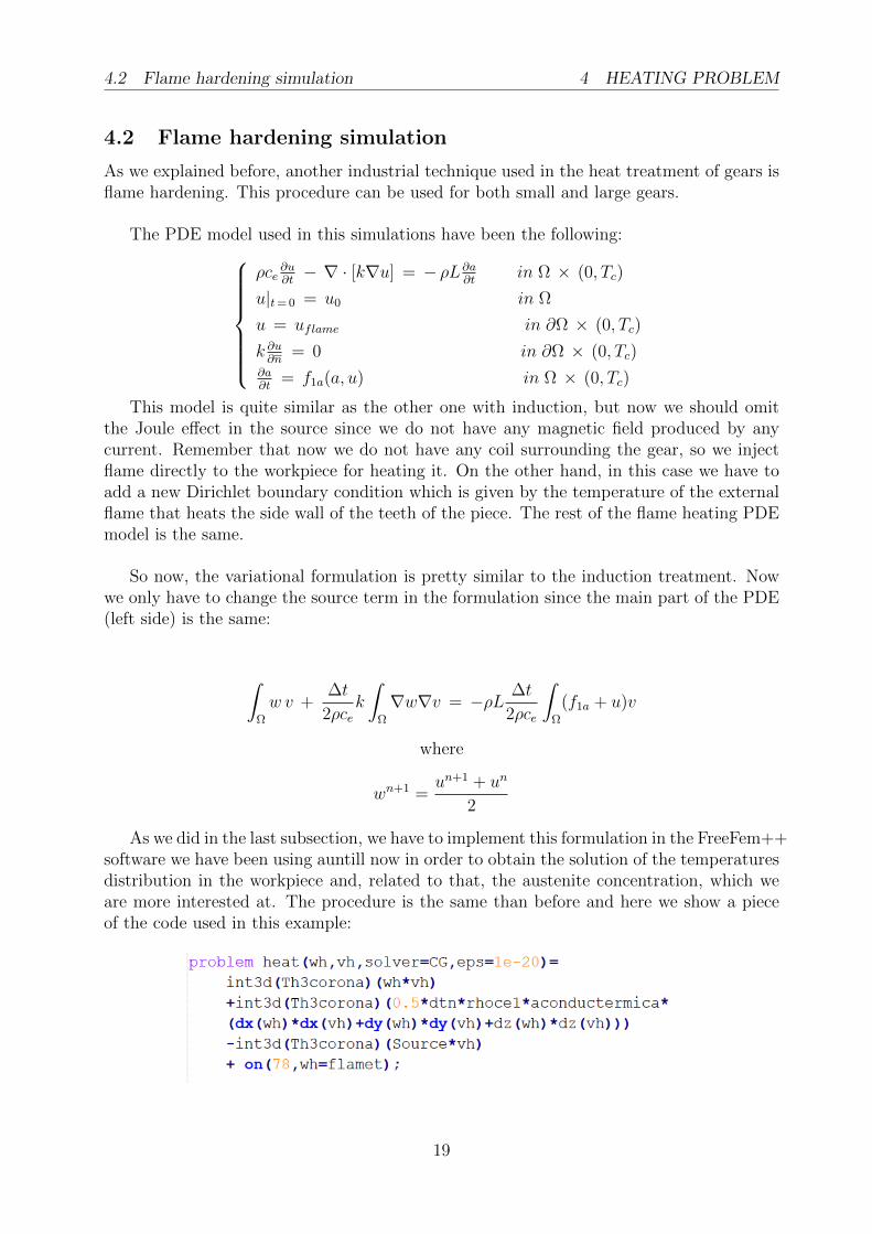
In the case of heating up with flame, we can see in the following figures that the amountof austenite has disappeared almost completely although it remains in the interior holesof the workpiece but in a so small proportion. On the other hand, the temperature hasbeen reduced significantly, although the piece remains quite hot inside, this is due to thecontact between water and the gear, because it emits energy to the water in the form ofheat. That situation makes the piece even hotter in the previous moments.
21
5 COOLING PROBLEM
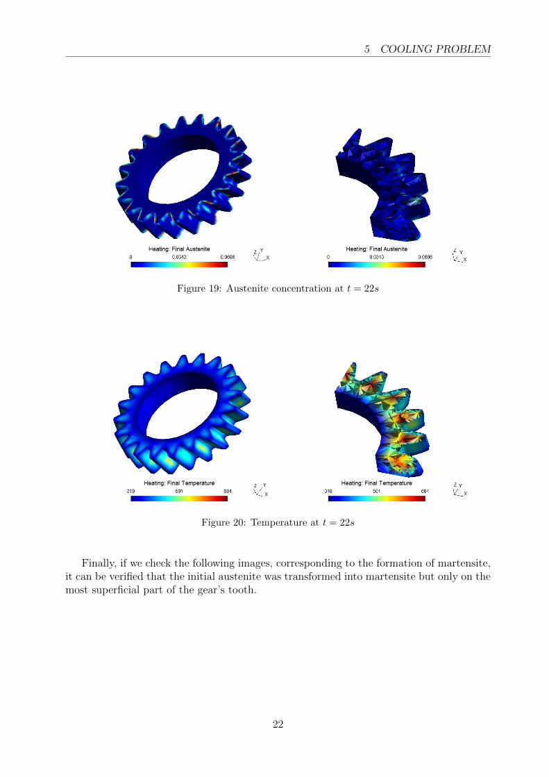
Figure 19: Austenite concentration at t = 22s
Figure 20: Temperature at t = 22s
Finally, if we check the following images, corresponding to the formation of martensite,it can be verified that the initial austenite was transformed into martensite but only on themost superficial part of the gear’s tooth.
22
5 COOLING PROBLEM
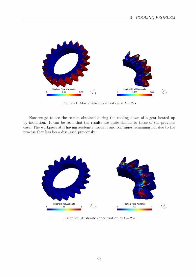
Figure 21: Martensite concentration at t = 22s
Now we go to see the results obtained during the cooling down of a gear heated upby induction. It can be seen that the results are quite similar to those of the previouscase. The workpiece still having austenite inside it and continues remaining hot due to theprocess that has been discussed previously.
Figure 22: Austenite concentration at t = 26s
23
5 COOLING PROBLEM
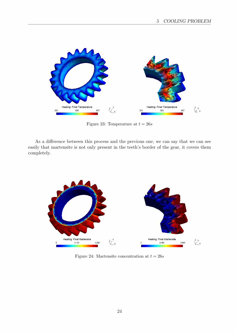
Figure 23: Temperature at t = 26s
As a difference between this process and the previous one, we can say that we can seeeasily that martensite is not only present in the teeth’s border of the gear, it covers themcompletely.
Figure 24: Martensite concentration at t = 26s
24

5 COOLING PROBLEM
Another way of inspecting the results of the simulation is by plotting the temperature ofsome relevant points inside the mesh as a function of time. By choosing four equally spacedpoints aligned inside a gear tooth, we obtain the diagram in figure 25. In this plot, point1 (purple curve) is the innermost point, whereas point 4 (yellow curve) is the outermostpoint.
400
600
800
1000
1200
0 5 10 15 20 25
Tem
pera
ture
(Ke
lvin
)
Time (seconds)
Evolution of temperature at four points inside the gear
"point1.dat""point2.dat""point3.dat""point4.dat"
Figure 25: Evolution of temperature at four points inside the gear
This diagram suggests that an interesting physical phenomenon is taking place insidethe gear: at the beginning of the cooling stage (t = 10 s), the temperature of points 1 and 3is counter-intuitively increasing, because austenite is releasing energy that had been storedin its crystal structure by the heating process.
25
6 CONCLUSIONS
6 Conclusions
In this work, we have used the finite element method to numerically solve simplified math-ematical models describing the industrial process of flame and induction hardening of steel.The results of our numerical simulations are in line with existing research [4], match ourphysical intuition and agree with experimental data. Moreover, they are stable with respectto the choice of time step and mesh resolution: a smaller time step and a higher resolutiondo not alter the qualitative aspect of the solution.
In this work, we’ve also described a complete workflow for the simulation of industrialprocesses using only free and open source software, namely FreeFem++ [3] and Tetgen [6]for FEA and mesh generation, Gmsh [2], Medit [1], and Gnuplot for visualization. Thisworkflow is summarized in figure 26, and can be adapted to different problems, not juststeel heat treating. We think that this kind of approach has the following merits:
• It’s flexible, because FreeFem++, besides doing finite element analysis, is also ageneral-purpose programming language (a C++ idiom). Therefore, all aspects of asimulation can be customized to suit specific needs by writing appropriate code.
• Parts of the workflow can be scripted, so that a program can automatically runmultiple instances of a simulation with different parameters or different geometry,then compare the results and keep the best one. This is a simple and effective, albeitcrude, approach to the optimization of an industrial process.
• The users are in full control: they can choose the finite elements type, the linearalgebra routines and the accuracy targets when the defaults are inadequate for theproblem that has to be solved. Moreover, they can inspect the internal data structuresused by FreeFem++ during the simulation and gain a deeper understanding of theunderlying numerical methods, as we have experienced ourselves during this work.
26

7 FUTURE WORK
Figure 26: Workflow
7 Future work
The heat source term due to eddy currents in our model of induction heating uses precom-puted coefficients for performance reasons. A more accurate simulation would describe theeddy currents using the vector potential formulation of Maxwell’s equations in the harmonicregime [5], and would therefore introduce the necessary geometry for the inductor and thesurrounding air, as can be seen in figure 27. Such a complex simulation would require someform of parallel computation in order to be feasible. In this regard, FreeFem++ providesaccess to effective domain decomposition techniques through the ffddm framework.
27

REFERENCES REFERENCES
Figure 27: Gear and coil surrounded byair. The air mesh density is higher nearthe coil and lower near its boundary.
Another area for improvement is the way timesteps and mesh resolutions are handled. In this work,we had to specify those parameters by hand, a time-consuming and error-prone process. A dynamic andadaptive choice would be ideal: the program could doonly as much work as needed in order to meet someaccuracy target, and the user would also be providedwith numerical estimates of the discretization errorsthat occur during the simulation.
References
[1] Pascal Frey. Medit: An interactive mesh visual-ization software. PhD thesis, INRIA, 2001.
[2] Christophe Geuzaine and Jean-FrancoisRemacle. Gmsh: A 3-d finite element meshgenerator with built-in pre-and post-processingfacilities. International journal for numericalmethods in engineering, 79(11):1309–1331, 2009.
[3] F. Hecht. New development in freefem++. J.Numer. Math., 20(3-4):251–265, 2012.
[4] JM Moreno, MT Montesinos, C Garcıa Vazquez,F Ortegon Gallego, and Giuseppe Viglialoro.Some basic mathematical elements on steelheat treating: modeling, freeware packages andnumerical simulation. Thermal Processing forGear Solutions, pages 42–47, 2014.
[5] JM Dıaz Moreno, C Garcıa Vazquez, MT GonzalezMontesinos, and F Ortegon Gallego. Analysisand numerical simulation of an induction–conduction model arising in steel heat treating.Journal of Computational and Applied Mathe-matics, 236(12):3007–3015, 2012.
[6] Hang Si. Tetgen, a delaunay-based quality tetra-hedral mesh generator. ACM Transactions onMathematical Software (TOMS), 41(2):11, 2015.
28


