STEEL COLUMN BEHAVIOUR IN FIRE CONDITIONS

STEEL COLUMN BEHAVIOUR IN FIRE CONDITIONS

by

Panayoula Braimi, Dip.Eng., M.I.Gre.E., M.N.F.P.A.

A thesis submitted in the fulfilment of the requirement for the Award of the Degree of Master of Philosophy in Structural Fire Engineering.

Unit of Fire Safety Engineering Department of Civil Engineering

University of Edinburgh September 1991

DECLARATION

This thesis is the result of research work for the degree of Master of Philosophy

undertaken in the Unit of Fire Safety Engineering, Department of Civil

Engineering and Building Science, University of Edinburgh.

It is declared that all the work and results in this thesis have been carried out

and achieved by the author herself and the thesis have been composed by her

under the supervision of Dr. E.W. Marchant and Dr. N. Fairbairn.

Dedicated to my family

ACKNOWLEDGMENT

This thesis is a synthesis of my association with many investigators. Among

the individuals whose contributions have greatly influenced me are

Professor Rotter, Head of the Department of Civil Engineering, who has

personally helped me technically and psychologically in my work; Dr. E. W.

Marchant, Director of Fire Safety Unit who made all the arrangements to

attend the seminars which was always an inspiring experience; Dr. D.

Drysdale, Reader in the Fire Engineering Unit, who with his enthusiastic

guidance partly supervised the research part of this thesis and provided

access to a thermal-analysis program; Dr. N. Fairbairn, lecturer in the

Department of Civil Engineering, who have patiently corrected my thesis

with his priceless experience and for offering me valuable suggestions; Dr.

A. Beard, researcher in the Fire Engineering Unit, who have helped me with

his valuable suggestions; Dr. J. Ooi, lecturer in the Department of Civil

Engineering, who helped me with various computing dificulties.

I am greatly indepted to Mr. H. L. Malhotra who have helped me be on the

right track and always ready to discuss vital matters in my thesis; Dr. I. Smith

who provided me with materials of great importance in my work and my

limitless indeptness to him for the arrangements he made for me to attend a

full-scale test at the Warrington Fire Research Centre in Cheshire. The

permission to attend this test by Steel Construction Institute is also noted;

The Fire Research Station staff, especially Mr. T. Morris, who have

generously allowed me to visit the FRS several times and have access to the

knowledge, experience, and library facilities at the FRS. Thanks to Dr. M.

Terro at FRS for his discussions with me, his encouragement and sustained

interest during the preparation of this thesis.

Thanks to SERC who finally covered my tuition fees for the last year of my

work.

V

Thanks are due to A. Ibrahim, H. Smith, H. Thompson, S. George, A. Duarte,

P. Worsdale and all the other colleagues and friends who have made my

stay here bearable.

Finally, I am deeply grateful to my parents who have funded and

encouraged me throughout my work with their selfless love. My brother

whose suggestions have greatly helped me surpass various difficulties living

in this country. My sister with her loving kindness and selflessness have

taken care of my affairs back home.

ABSTRACT

Urban development has given rise to taller and more extensive buildings

whose contents are of increasing commercial value and these offer an

increasing risk to life at the same time. Therefore buildings should offer

some resistance to the destructive effects of fire. These have led to the

incorporation of design features to facilitate escape and in recent times

resistance to the effects of fire. The practical features of the building which

are involved in all these are walls, doors, floors, passages, corridors, beams,

stairs, and columns. This project considers the study of columns exposed to

standard fire tests (to BS 476 or to ISO 834), natural fires or real fires. The

columns were pin-ended and axially loaded without applied moments.

TASEF-2 (Temperature Analysis of Structures Exposed to Fire) is a finite

element computer program which has been used for calculating the

temperature profiles throughout sections at any given time. Verification of the

model has been done by comparing its results with those of experimental

tests.

The column structural response to loading, which may be in terms of

deflection or load bearing capacity is assessed using the following Codes:

Eurocode 3: Part 10 [Eurocode 3, 1990], European Recommendations for

the Fire Safety of Steel Structures [ECCS,1983], BS 5950:Part 8: 1990 [BSI,

1990] and the Swedish Code [Pettersson, 1976]. Critical comparisons of the

different Codes are also given and their advantages and disadvantages are

discussed.

vii

CONTENTS

ACKNOWLEDGEMENTS V

ABSTRACT VU

CONTENTS Viii

CHAPTER ONE Introduction 1

1.1 The fire and its cost 1

1.2 Metal load-bearing structures 1

1.3 The structural fire protection 2

1.4 The objectives of this work 5

1.5 Future trends 6

PART I Thermal Problem 8

CHAPTER TWO Physical and Thermal properties 9

2.1 Physical Properties 9

2.1.1 Density 9

2.1.2 Thermal strain 9

2.1.2.1 Variation of thermal expansion with temperature 10

2.2 Thermal Properties 15

2.2.1 Thermal Conductivity 15

2.2.2 Specific Heat Capacity 19

2.2.3 Thermal Diffucivity 21

2.2.4 Thermal Inertia 21

CHAPTER THREE Heat transfer analysis 24

3.1 Mechanisms of Heat Transfer 24

3.1.1 Theoretical Model 24

3.2 Temperature Analysis of Steel Columns 28

3.2.1 Standard fire tests 28

3.2.2 Full scale tests 33

3.2.3 Existing Computer Programs 38

3.2.4 Existing Codes 47

3.3 Example 50

Viii

PT II Structural Problem 76

CHAPTER FOUR Mechanical Properties 77

4.1 Stress and Strain - Axial Loading 77

4.1.1 Stress-Strain Diagram at room temperature 77

4.1 .2 Stress-Strain Diagram at high temperatures

Modulus of Elasticity 82

4.1.2.1 Effect of temperature on flow stress 82

4.1.2.2 Testing Methods 84

4.1.2.2.1 Static Methods 84

-Tests under steady-state heating conditions

-Tests under transient heating conditions

-Discussion

4.1.2.2.2 Dynamic Methods 106

4.1.2.2.3 Suggestions 109

4.2 Tensile strength 109

4.3 Residual stress 109

4.4 Modelling Steel Behaviour 112

4.4.1 Thermal strain 113

4.4.2 Instantaneous stress related strain 113

Comments

Existing Computer Programs

Codes

4.4.3 Creep Strain 128

Comments


Codes

4.4.4. Total Strain 136

CHAPTER FIVE Design of Steel Columns In a Fire Environment 137

5.1 Fire resistance periods 137

5.1.1 Building Regulations 137

5.1.2 The Time Equivalent Calculation Method 138

5.2 Codes related to the Performance of Constructions in Fire 143

5.2.1 BS 5950:Part 8. Code of Practice for Fire Resistant Design 143

5.2.1.1 Fire Resistance derived from testing 144

IX

X

5.2.1.2 Fire Resistance derived from calculation 145

5.2.1.2.1 Limiting temperature method 146

5.2.1.2.2 Design temperature 148

5.2.2 European Recommendations for the Fire Safety of Steel Structures. 149

5.2.2.1 Deformation Behaviour

Limit state of deformation 150

5.2.2.2 Ultimate Load Bearing Capacity

Limit state of failure 152

5.2.2.3 Buckling of steel columns 153

5.2.2.4 Critical Temperature of columns 158

5.2.3 Fire Engineering Design Manual 161

5.2.4 Discussion 188

CHAPTER SIX Design Example 197

6.1 BS 5950:Part 8:Code of Practice for Fire Resistant Design. 200

6.1.1 Centre Column 210

6.1.2 Edge Column 220

6.2 European Recommendations for the Fire Safety of Steel Structures. 230

6.2.1. Centre Column 230

6.3 Swedish Institute of Steel Construction 238

6.4 Fire Protection Insulation 247

6.5 Conclusions 249

CHAPTER SEVEN Conclusions-

Suggestions for future work 252

Appendix A: BSI. Structural use of steelwork in building.

BS 5950: Part 8:1990. Code of practice for fire resistant design 257

Appendix B: Eurocode No.3. Design of steel structures

Part 1: Draft 1990. Structural design.

ECCS - Technical Committee 3 - Fire Safety of Steel Structures 262

Appendix C: Swedish Institute of Steel Construction

Fire engineering Design of Steel structures [Pettersson, 1976] 270

Appendix D: Fire Protection Insulation [ASFPCM, '88] 282

References 284

1

CHAPTER ONE Introduction

1.1. The fire and its cost

The fire and its cost have increased over the centuries as society and

technology have evolved. The concentration of people in towns and the

growth of industries which handle flammable or explosive products such as

oil, synthetics and chemicals increase the scale of fire risk.

Fire risk affects both human life and property.

The first category of risk can hardly be calculated in monetary terms. The

statutory texts usually provide information to prevent loss of life in a fire

incident.

In the case of damage of material goods as a result of combustion, corrosion

or plant failure caused by high temperatures, it is the insurance company

that defines the risks and determines premiums.

The possible effect of fire on the natural and social environment is a very

important matter as well. A fire in industrial premises can lead to

redundancies, while a fire in an oil refinery can result in pollution which is

hazardous to the surrounding population.

1.2. Metal load - bearing structures

Though a number of different metals are used to some extent in building,

only iron and steel (and to limited extent in recent years aluminium) are

normally used for those parts which have to carry a load. They are not

combustible and they present no risk of fire spread from direct burning. On

the other hand, unprotected metal surfaces heat up in a fire and may cause

fire spread by conduction. Load-bearing structural elements of unprotected

metal collapse when excessively heated. Structural steel begins to loose

strength above approximately 200300 0C but how quickly structural steel

fails depends on its redundancy and degree of restraint. When metals are

heated, they expand. In a framed building, the failure of a single structural

element will only cause local collapse. To reduce the chance of collapse,

structural steel should be usually protected by a layer of non-combustible

heat-insulating material.

The author's area of research is concerned with unprotected steel columns.

The advantages of unprotected steel are reduced cost , specialist fire

protection contractors are not required on site, less floor space is used,

erection is fast and a good resistance to mechanical impact is achieved.

A Digest [BRE, 1986] published by the Fire Research Station states that

large columns have a half-hour fire resistance inherently, without

protection, provided the ratio of fire-exposed perimeter to cross-sectional

area is sufficiently low ( 50m 1 or less). Smaller columns achieve the half-

hour rating by using some form of protection, for example by filling the void

between the flanges of the columns with a single layer of autoclaved aerated

concrete blocks which protect the web and the inner flange faces from heat.

1.3. The structural fire protection

Fire safety systems are normally designed to minimize the occurence of a

disastrous fire and hazard potentials which are referred to as loss of lives,

property, use and environmental mishap. Fire safety can be provided by

active or passive measures or a combination of both. The active measures

come into operation on the occurence of a fire. They comprise fire detection

and fire control systems. The passive measures are part of the built system

and are functional at all times. They include building layout, design and

construction. Measures may interact, the provision of the activation of a

system can have beneficial effects on another. It is difficult for the designer to

decide how safe the project is going to be, to distinguish the relative

importance of fire safety strategies and to find out about the trade-offs

involved.

2

The safety of a structure against fire - one of the fire protection strategies - is

governed by:

a' the risks involved in case of a severe fire considered as an accidental

situation,

b/ the risk-reducing effect of conventional measures,

Cl the risk-reducing effect of non-structural measures such as detection,

alarm systems, sprinkler systems.

The provision of non-structural measures may result in a reduced level of

structural fire safety becoming acceptable.

Structural fire protection engineering involves the design of structural

building elements to resist the effect of fire. For individual structural

elements, an increase in resistance is achieved by increasing member size

or by providing adequate insulation in the case of steel and by increasing

the thickness of concrete around the reinforcing and prestressing steel in the

case of concrete.

Historically, the basis of the measurement of fire resistance for structural

elements and assemblies has been the standard fire resistance test. A major

difficulty with using the standard fire resistance tests' results or predicted

results is that the response of full size assemblies to real fires cannot be

measured. In recent years, there has been several attempts to predict test

results by calculation as full scale testing is not practical.

In order to predict the response of a structure in a fire, three basic

components has to be considered:

the fire,

the heat transfer to the structural members,

the affect of elevated temperature on structural performance.

The above components are not independent, they are interrelated in a very

complex manner. A design method requires realistic simplification of the

3

complex problem in a manner which will yield consistent results with known

levels of reliability.

Because the steel structural system has virtually no impact on a

compartment fire, one can isolate the fire from the other two basic

components (the heat transfer to the structural elements and the resulting

structural performance). There are computer programs that predict the

development of a fire and its different phases. In this research work, the

temperature-time curves presented in literature such as the standard

temperature-time curve or the hydrocarbon curve adopted by the U.K.

Department of Energy are only used.

Once the fire is defined, the temperature distribution in the structure must be

determined. The heat transfer problem is very complicated and the modes of

heat transfer are dependent on the type of structural system. Different

materials have different thermal protective systems. In the case of structural

steel, three main systems are usually considered:

unprotected steel,

insulated steel,

membrane protected steel (such as suspended ceiling).

Usually, there are difficulties related to the input of data concerning the

material properties of the insulating material because there is limited

information on their temperature dependent material properties such as the

density, conductivity and specific heat of the material.

The most difficult case to model is the membrane protected steel because in

addition to the heat transfer properties, its thermal performance depends

strongly on its integrity.

The behaviour of unprotected steel in a fire has been investigated using the

model TASEF-2 [Sterner, 1990] to model the heat transfer from the fire to the

unprotected structural steel. Results obtained using TASEF-2 are presented

in Chapter Three (3).

4

Once the time dependent temperature gradient in a structural member has

been determined, the effect on the structure may be analysed. A structure is

said to have failed if either the ultimate limit or the serviceability limit is

reached.

A serviceability limit is reached if the strains or the deflections are such that

the columns deflect excessively producing an unsightly appearance.

The ultimate limit state is reached if excessive local damage causes

deterioration of the material to such an extent that plastic hinges begin to

form around the structure, reducing the statically indeterminate structure to a

mechanism.

The response of steel columns to high temperatures was studied using

different design Codes. No existing computer program was made available

to the Unit for implementation and further conversion at a reasonable price.

This is the reason why a computer program is not used for the structural

analysis.

Non-linear instability effects are excluded from this study.

1.4 The objectives of this work

The author's research work focusses on steel columns and their behaviour

in a fire environment. The study of three cases is presented in Chapter

Three(3). These cases are:

a universal column exposed to fire from four sides in a fire

compartment,

a universal column built next to a wall in a fire environment,

a universal column built into a wall which is part of a boundary which

belongs to a fire compartment.

In the existing computer programs, the thermal analysis is not integrated with

the mechanical analysis. Sometimes, the thermal and mechanical analyses

are carried out using different programs. According to such analyses, the

time-temperature of the steel structures is calculated and is used as an input

information for the analytical prediction of the mechanical behaviour. This is

the reason why this thesis is divided into two parts elaborating the thermal

and structural behaviour of columns respectively.

In the first part of the thesis (Part I), correlations are made among the

standard tests' results taken from "The Compendium of U.K. Standard Fire

Test Data" [Wainman, 1988] , the theoretical results obtained by using the

computer program named TASEF-2 (Temperature Analysis of Structures

Exposed to Fire) and the Pettersson's method [Pettersson, 1976].

Correlations between full scale test results [Almand, 1989] and results from

TASEF-2 are presented as well.

In the second part ( Part II ), the existing Codes are presented and analysed.

The existing Codes studied are:

- BS 5950: Part 8: Code of practice for fire resistant design

[BSI, 1990],

- ECCS: European Recommendations for Steel Structures

[EGGS, 1983],

- Swedish Code for Design of Steel Structures [Pettersson, 1976].

A design example using the above Codes is presented in Chapter 6. Non

linear instability effects are excluded.

15 Future trends

The computer programs have still to be developed.

Unknown mechanical properties of various building materials at elevated

temperatures must be investigated in different fire conditions and be used as

input to the structural programs.

E.

A three- dimensional framework program to take account of fire will be an

important development of the existing computer programs.

Factors like plastic hinge rotation, finite deformations leading to the problem

of buckling and instability in individual members and in part or all of a

framework must be investigated further and incorporated in the analysis of

the computer programs.

7

RAM 1: Thermal Problem

Mm

1,

C

I,

CHAPTER TWO Physical and Thermal Properties

The material properties can be divided into four groups [Malhotra, 1982]:

-Chemical (decomposition, charring),

-Physical (density, expansion, softening, melting, spalli ng),

-Mechanical (yield strength, elasticity, tensile strength, creep),

-Thermal (thermal conductivity, specific heat capacity, thermal diffusivity,

thermal inertia).

In the case of steel, the chemical properties are not of interest - only wood is

subject to decomposition and charring. Softening of steel will occure at

temperatures higher than 800°C. Melting of steel is unlikely to happen at the

maximum temperatures (1200'C) usually experienced in fires.

The discussion of the mechanical properties is given in Chapter Four of this

study.

2.1 Physical Properties

2.1.1 Density.

For all steel qualities, the value of p=7850 kg/M 3 should be taken for the

calculations, regardless of the temperature history.

2.1.2 Thermal strain.

When a material is heated, its thermal movement depends on the coefficient of

linear expansion and on the restraint imposed on its ends. If the material is

unrestrained and under constant temperature, there is no stress associated with

the strain. Where the material is restrained, for materials that follow Hooke's

law in the elastic range - like metals - there is less complication than for

inorganic composite materials where Hooke's law does not apply due to

cracking and phenomena associated with loss of water and phase changes in

the cement matrix and aggregate upon heating.

10

If the temperature of the solid material is raised by T,the material elongates

according to the equation:

L=L0( 1 +T+a1 T2+cz2T3 ) ( 2.1)

where:L=length under a temperature rise of T,

L0=length at the initial temperature,

a=coefficient of thermal expansion.

For most purposes, the following equation is adequate:

L=L0 ( 1 +czT) (2.2)

This happens because, for pure metals, the constants a,a 1 ,a2 have values

10-5 ,10-11 ,10-14 respectively and the values of a l A2 are considered negligible

in comparison with a. The coefficient of thermal expansion is determined in

tests under stress-free conditions.

According to BS 5950: Part 1:1985 the coefficient of thermal expansion at

ambient temperatures is defined by a=1 .2x1 0?C.

2.1.2.1 Variation of thermal expansion with temperature

The coefficient of thermal expansion depends on steel temperature. In 1953, the

National Physical Laboratory reported on the thermal movement of 22 different

steels at elevated temperatures (Cooke, 1988). The research was sponsored by

the British Iron and Steel Research Association. According to this research, for

steel with a carbon content of 0.23% - which is nearest to structural steel in

chemical composition - the coefficient of thermal expansion varies from a mean

value of 12.18x10 6fC in the range 0-100°C to 14.81x10 6/°C in the range of 0-

1200°C. Because structural steel begins to lose strength at temperatures above

550°C, the temperatures of main interest are in the range 0-550 °C over which

11

the mean value of the coefficient of thermal expansion is a=14.1 7x1 6

(Cooke,1988). From the same reference and for temperatures greater than

700°C, it is observed that the coefficient of thermal expansion reduces with

further increase in temperature. This phenomenon is called phase

transformation, it is caused by the transformation of pearlite to austenite and is

accompanied by a rearrangement in the atomic structure from the body -

centred cubic structure to the face-centred cubic structure (Fig. 2.1 )[Walker

J.,1984 - Kennedy R. et al., 1970]. The magnitude of the actual shrinkage and

temperature of onset of phase transformation depend on the chemical

composition ( Fig. 2.2). According to tests that BSC were commissioned to

conduct, the variation of heating rate does not affect the temperature at which

the phase transformation commences and ceases but does affect the

magnitude of shrinkage (Fig.2.3.). A high precision MMC High Speed Vacuum

Dilatometer was used for these experiments. Two specimens were taken from

the same piece of structural steel containing 0.28% C and 0.67% Mn. It is

certain that ignorance of phase transformation leads to strain overestimate at

temperatures where the onset of phase transformation occurs. However, in

practice, the steel structural members fail before reaching the phase

transformation temperature. In that case, phase transformation is not considered

as sufficiently an important factor to affect the behaviour of structural steel.

Codes

The European Recommendations for the Fire Safety of Steel Structures by the

European Convention for Constructional Steelwork (1983), BS 5950:Part

8:1990,and Eurocode: Part 10,1990: Structural Fire Design consider, as an

approximation,that the coefficient of thermal expansion is independent of steel

temperature and may be taken as a=14x10 6fC. ECCS recommends this value

for the grades of steel Fe 310, Fe 360, Fe 510 as specified in the Euronorm 25-

72. BS 5950 recommends it for hot finished structural steels that comply with BS

Ferrite B.C.C. Austenfte F.C.C. Fig. 2.1 Crystal structures of iron (Kirby, 1986)

130

120 OOG%C F cllO

1 00

90 NO 800 900 1000

Temperature °C Fig. 2.2 Thermal expansion - temperature curves

for low and medium carbon steels in the

phase transformation range (Cooke, 1988).

50OC/min heating and cooling rate

10°C/min 10*C/min heating and cooling rate 1.50

1.25

.00 C

!0.75 CO

0.5C

0.25

n•__ I - S I I I -.

0 100200 300 400 500 600 700 800 9001000 Temperature °C

Fig. 2.3 Dilatometer curves for a mild steel

showing effect of different heating

and cooling rates (Cooke, 1988).

12

13

4360 at elevated temperatures. EC3 recommends that this value is valid for

steel qualities Fe 310,Fe 360,Fe 430,Fe 510 as specified in the Euronorm

10025 and for Fe 460 as specified in EN 10113. In all other cases the reliability

of the given design values must be demonstrated explicitly.

As an alternative, EGGS advises that the thermal elongation may be calculated

by the following equation:

¶=0.4x1 0 86 2+i .2x1 05O-3x1 0-4 (2.3)

where: 1= length at room temperature

AI= temperature induced expansion

steel temperature

The equation is illustrated in Fig. 2.4 for a practical temperature range. It does

not illustrate the phenomenon of phase transformation.

EC3 recommends ,for more explicit design, that the thermal elongation may be

as well given by:

16

1

11 6x1 0+i .2x1 0 5O 2

Al T1 1x103

0 3+2x1 o9

for O:5 750°C

for 7500C<9 <8600C

for 860°C<O<1 200°C

(2.4)

where: l=length at room temperature (m)

Al=temperature induced expansion (m)

O=steel temperature (°C)

The graphical representation of elongation varying with temperature is given in

Figure 2.4. It does take into account the phase transformation by defining the

coefficient of thermal expansion as a constant equal to 11x10 3 over the

temperature range 750°C - 860°C.

14

/1 -recommended Al

-

alternative

1.2

0.E C

0.4

0.2

0 200 400 600 800

steel temperature in °C

Fig. 2.4 Thermal expansion of steel as a

function of the steel temperature

(ECCS, 1983).

15

2.2 Thermal Properties

The thermal properties of materials which affect their behaviour when

exposed to fire are:

- thermal conductivity;

- specific heat capacity;

- thermal diffusivity;

- thermal inertia.

2.2.1 Thermal Conductivity

Thermal conductivity characterizes the capability of various materials for

transmitting heat. In buildings, the materials may experience three modes of

heat transfer which are:

- thermal conduction by atomic and molecular vibration;

- thermal conduction by radiation;

- thermal conduction due to mass transfer (gaseous conduction).

The bonding between the molecules of an element influence its ability to

transmitting heat when subjected to a heat flux. The heat energy is

transmitted by very high frequency elastic waves. Because the frequency of

variation for rigidly-bound molecules is high, the rate at which the energy is

transferred is also high. The weakly- bonded molecules pass less heat

energy through their bulk than the rigidly- bonded ones. The quantom of

energy associated with such wave motion is called the phonon. A metal is

considered to be a good conductor because the electrons move from

regions of high temperature to regions of low temperature. In an insulation-

type material, the conduction is dominated by phonon-phonon collisions or

phonon-lattice framework collision processes.

With an increase in temperature, the interaction between phonons increases

and. causes the thermal resistance to increase. So, the thermal conductivity

decreases with an increase of temperature.

Surfaces which have a temperature above absolute zero are capable of

transmitting and absorbing radiation. This happens because when radiation

passes through solids, it undergoes scattering at structural imperfections,

crystal boundaries and pores.

According to Stefan Boltzmann's law, the total emissive power by unit area

of a black body is given by:

E=aT4 kW m(2.51 (2.5)

where: a=56.7x10 12 (Stefan-Boltzmann Constant),

T=temperature ( °C).

A black body is a surface which absorbs all radiation incident upon it.

This type of conductivity becomes quite significant at temperatures above

500°C for highly porous materials. For opaque-type materials, it becomes

significant at about 1000 °C or above.

In a material under thermal gradient with pores which are filled with air, the

air can ease the heat energy to pass through the material. It has been shown

that for a porous material the gaseous conduction component of the thermal

conductivity makes a moderate contribution to the overall conductivity

compared to the radiant component.

The thermal conductivity varies with temperature,density and moisture

content. Example of the variation of thermal conductivity with temperature

and density are given in Figures 2.5,2.6 respectively.

When water displaces the air in the pore spaces, the thermal conductivity of

a porous-type material becomes greater.

16

I Only.

ous jChon

17

U oo oo WO

9

Fig. 2.5a Variation of the thermal conductivity with temperature for a

medium - density fibrous insulant (Shield, 1987)

23

20

A Wth' k'

15

aggregate (Quartz.)

200 400 600 800 1000

'°c

Fig. 2.5b Comparison of thermal conductivity variation with temperature

for amorphous and crystalline materials ( Shield, 1987).

12

/

18

vYm k Li1

0 500 OOO 1500 20W

_.B_ Dry Bulk Density kgn 3

Fig. 2.6 Variation of thermal conductivity for porous materials with

density ( Shield, 1987).

BS 5950 :Part 8 [BSI,1 990] recommends for the thermal conductivity of hot-

finished steels (complying with BS 4360) a value of 37.5 [W/m °C]. This

value is independent of temperature and is to be used in the fire

calculations.

2.2.2 Specific Heat Capacity

Specific Heat Capacity is the quantity of heat that must be supplied to a unit

quantity of substance in a particular process in order to change the

temperature of the substance by one degree. Since the unit quantity of

substance may be different e.g. 1 kg, 1 mole, 1m 3,a distinction is made

between the mass specific heat (J/kg K), the molar specific heat (J/mol K)

and the volumetric specific heat (J/m 3 K).

The variation of the specific heat capacity with temperature for chemically

stable materials is given in Figure 2.7a. The same relation for complex

materials such as gypsum is given in Figure 2.7b. It can be seen that the

specific heat increases up to the temperature of 100 °C which is the boiling

point. This happens due to the removal of water and vapour in the pores,

making the energy needed to raise 1 kg of a material by 1 K at this

temperature much greater than would normally be the case.

EGGS [ECCS,1983] recommends, as an approximation, that the specific

heat be considered independent of the steel temperature. In calculations

and for all grades of steel, it may be taken as:

c5 =520 (J/kg °C)

The same document gives an analytical relationship for the specific heat

capacity to be determined as a function of temperature. The equation is:

19

c= 38 x 10 -5 0 2 + 20 x 10 -2 0 + 470 [rn/rn] (2.6)

C o

J k R'

x 10

Cp

.jkg k

x 10 3

20

200 400 600 800

oc Fig. 2.7a Variation of specific heat capacity of chemically stable

materials (Shield, 1987).

Fig. 2.7b Variation of specific heat capacity of gypsum with temperature

(Shield, 1987).

21

The relationship is illustrated in Figure 2.8 for a practical temperature range.

The dashed line in the same figure represents the approximation of a

specific heat capacity value independent of temperature.

BS 5950: Part 8 [BSI, 1990] recommends that a value for the specific heat

capacity of hot finished structural steels (complying with BS 4360) of 520

[J/kg °G] be used in fire calculations.

2.2.3 Thermal Diffusivity

Thermal Diffusivity is a measure of a material's ability to conduct heat energy

in relation to its thermal storage capacity. It also gives a measure of the rate

at which thermal energy can travel through a material which in turn controls

the rate of temperature rise within the material.

The thermal diffusivity may be defined as follows:

thermal conductivity of material (2.7) PCP

density of material xspecific heat of material

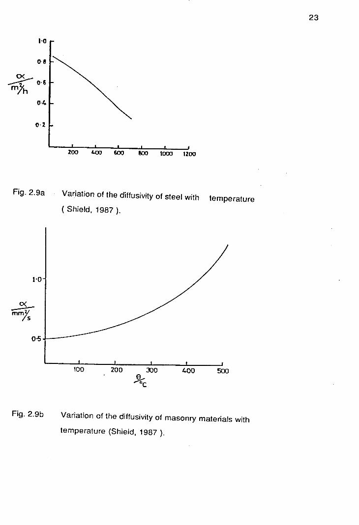
The variation of the diffusivity of steel with temperature is given In Figure

2.9a,b. EGGS [EGGS, 1983] recommends density a value of 7850 kg/m 3

This value is independent of temperature and valid for all grades of steel.

2.2.4 Thermal Inertia

Thermal Inertia may be defined as the product of thermal

conductivity,density and specific heat capacity (ApC). It can be easily

calculated if the variation of thermal conductivity and specific heat with

temperature are known.

1 00

900

43 800

700 U,

0

600

500

—._—_—....recommended

alternative

22

0 200 400 600 800

steel temperature in °C.

Fig. 2.8 Specific heat of steel as a function of the steel temperature

(ECCS, 1983).

t•0

m)1t

O•4

0-2

_.x. piij

Fig. 2.9a Variation of the diffusivity of steel with temperature

(Shi&d, 1987).

23

10

4: 05

100 200 300 400 500

Fig. 2.9b Variation of the diffusivity of masonry materials with

temperature (Shield, 1987 ).

CHAPTER THREE Heat transfer analysis

3.1 Mechanisms of Heat Transfer

Three basic mechanisms of heat transfer can be distinguished:

- conduction;

- convection;

- radiation.

Conduction is the method of heat transfer effected by microparticles of

bodies (molecules, atoms and electrons) which possess different levels of

energy and can exchange this energy as they move and interact. It is the

basic mode of heat transfer within solids. It occurs in gases and liquids but it

is not the principal mode of heat transfer.

Convection is the transfer of heat by the mass of a liquid or gas as it moves

from a region of one temperature to a region of a different temperature. It is

the basic mode of heat transfer for liquids and gases.

Radiation is the process of transfer of the internal energy of a body in the

form of radiation energy. It requires no intervening medium between the

source and the receiver.

Under real conditions, heat transfer often occurs by two or even three

mechanisms simultaneously.

3.1.1 Theoretical Model

The non-linear heat flow equation must be solved to predict the distribution

of the temperature in the structure exposed to fire.Because analytical

solutions of such equations exist only for idealized cases, finite element or

finite difference methods must be employed to approximate heat conduction.

The governing equations for heat conduction are given below:

- the heat balance equilibrium equation

_vTQ+êQ=o : (3.1)

24

25

- the Fourier law

(3.2)

where:

g = the heat flow vector, ae

e= = the rate of specific volumetric enthalpy change, at

Q= the rate of internal generated heat per unit volume,

= a symmetric positive definite thermal conductivity matrix,

T= temperature,

t= time,

= the gradient operator.

From the above:

_vT(kvT)+eQo (3.3)

For isotropic materials, the thermal conductivity matrix is given as follows:

k=kl (3.4)

where:

1= the identity matrix

The specific volumetric enthalpy is defined as follows:

T

e= fcpdT+1 1 T0 (3.5)

where:

T0= the reference temperature (usually zero),

C= the specific heat,

p= the density,

26

1 1= the latent volumetric heat due to phase changes at various

temperature levels

The time derivative of the above equation is:

(3.6)

aT where: T= = the rate of temperature change

Substituting, the conventional form of the transient heat flow equation is

given as follows:

_VT(kVT) + C P -j- _ Q0

(3.7)

In order to solve the above equations, one must specify initial and boundary

conditions.

An initial condition is given by specifying the distribution of temperature in a

body at zero reference time.

Boundary conditions are given as temperature or heat flow on parts of the

boundary (aVT and aVq respectively):

av = aVT + aVq (3.8)

where:

T= T (x, y, z, t ) = temperature,

qn= nT a = T = prescribed heat flow,

with 11 = the outward normal to the surface.

Heat transfer phenomena it is difficult to model. If approximate formulas are

used the convection and radiation heat transfer is given by the equations.

27

The convective heat transfer is given as follows:

3 (T - Tg)Y

(3.9)

where:

qn =the rate of heat transferred by convection,

y =the convection factor and power respectively,

TS =surface temperature,

T =surrounding gas temperature.

The radiation heat transfer is given as follows:

C (TS4 - T54 )

where:

a =the Stefan-Boltzmann constant,

T =absolute surface temperature,

T =absolute surrounding gas temperature.

Cr =resultant emissivity

(3.10)

The resultant emissivity depends on the surface properties and geometric

configuration. In fire engineering design, when assessing radiation between

flames and structures, it may be assumed for the calculation that the case is

similar to radiation between two infinitely long parallel planes. For the latter

case, the emissivity is given by the following equation:

1 Cr= i

-+- - 1 C Eg

where:

Cg= appropriate gas or flame emissivity.

The total heat flux at a boundary is calculated as follows:

A A A q=qC + q' (3.12)

3.2 Temperature Analysis of Steel Columns

The temperatures attained by a structural element may be assessed in four

different ways:

- conducting a standard fire test;

- conducting a full scale test;

- using the codes;

- using the existing computer programs.

3.2.1 Standard tire tests

The fire resistance of load bearing structural elements is currently assessed

in the U.K., in accordance with the British Standard 476: Part 20,21 22

[BSI, 1987]..

Generally, a fire resistance test is carried out on a specimen which is as far

as possible, representative of the structural element in terms of its size,

materials and workmanship.

Loads are also applied to simulate the same magnitude and type of stresses

generated in practice.

The test specimen is heated in a gas fire furnace in which the temperature is

controlled to vary with time in accordance with the BSI recommendations

[BSI, 1987]. The fire test is terminated either at the request of the sponsor or

when the limiting requirements for maintaining the relevant criteria for

stability, integrity, insulation are achieved. At the end of the heating period,

as previously defined, the loads applied to the structural element under

consideration may be removed and reapplied after twenty four (24) hours.

The reload test is optional. If collapse occurs dunng the test procedure, the

28

0.68 is

0.60 m

0.60 is

0.60 is

0.60 is

Exposed length 3.08 is

I flange width

Fire Fire

& flange width

Fire Concrete cap

Fire

TRANSVERSE SECTION

I DATA I SHEET NUMBER 40a

DIMENSIONS AND PROPERTIES

Column

29

SECTION DIMENSIONS MASS DEPTH WIDTH THICKNESS ELASTIC MODULUS OF

PLASTIC MODULUS MOMENT OF INERTIA SERIAL SIZE 41D PER OF

WEB FLANGE AXIS AXIS AXIS AXIS AXIS AXIS AND TYPE PROPERTIES METRE SECTION SECTION XX YY XX YY XX YY

sin

NOMINAL

kg

198

mis

339.9

mm

314.1

sin

19.2

mm

31.4

cm3 cm3 cm3 cm3 cm4 cm4

305 x 305 2991 1034 3436 1516 50832 16230

COLUMN ACTUAL 341 314 * * 1

CHEMICAL COMPOSITION (PRODUCT ANALYSIS - Wt.Z) (*)

SECTION STEEL QUALITY C Si Mn P 5 Cr Mo Ni V Cu Nb Al N I - _I -+-------+-----+- I I -_I_•-+ -I-

COLUMN GRADE GRADE 43A I I I I I I I I I I

ROOM TEMPERATURE TENSILE PROPERTIES (*)

NOTES

POSITION LYS N/mm2

TS N/mm2

ELONG Z

FLANGE

TEST CONDITIONS

EXPOSED LENGTH : 308 cm EFFECTIVE LENGTH 215.6 cm RADIUS OF GYRATION (y—y) : 8.02 cm SLENDERNESS RATIO : 26.88 MAXIMUM AXIAL STRESS 144 N/mm2 AREA OF CROSS SECTION : 252 cm2 MAXIMUM LOAD : 3629 kN LOAD APPLIED : 3630 kN

After 20 minutes the loading frame collapsed, thereby prematurely terminating the loaded fire test. At that time the section had bowed approximately 10 mm. However the heating cycle was continued until 33 minutes Temperatures accurate to the nearest 5 deg. C Initial ambient temperature = 10 deg. C

(*) Data not available

THERMOCOUPLE _POSITIONS

Concrete base (Not to scale)

VERTICAL SECTION

30

TEST CENTRE : FIRTO -- BORE}IAfIW000 TEST DATE : 17th. MARCH 1980 TEST NUMBER TE 3646

88 476 PART 8 : 1972 ASSESSMENT

RE-LOAD TEST SATISFIED STABILITY : 20 MINUTES (a) FIRE RESISTANCE 20 MINUTES

DATA SHEET 40b NUMBER

HERJIOCOUPLE TEMPERATURE Deg. C AFTER VARIOUS TIMES (MINUTES) (b) OCATION ----------------- - --

3 6 9 12 15 18 21 24 27 30 33

50 85 140 215 300 380 465 530 585 625 665 XPOSED Fl LANCES F2 40 70 140 210 300 395 485 560 620 660 700

F3 30 75 145 240 320 445 540 610 660 695 725 F4 30 85 150 230 345 405 490 565 620 665 700 F5 35 75 130 200 280 360 435 495 560 610 650 E6 30 60 120 200 285 375 455 520 590 635 670 F7 40 75 150 235 305 410 495 570 640 680 715 F8 35 90 155 240 330 405 475 535 600 635 670

MEAN 35 75 140 220 310 395 480 550 610 650 685

XPOSEI) WI 50 95 160 255 360 445 525 590 645 690 725 EB W2 45 80 145 245 345 445 535 605 650 685 715

143 40 80 145 250 365 470 555 630 685 720 740 144 45 115 185 280 390 475 560 630 685 715 740

45 95 160 260 365 460 545 615 665 705 730 MEAN

435 500 620 730 740 765 795 810 835 830 845 LEAN FURNACE GAS

TANDARD CURVE (c) 492 593 653 695 729 756 779 799 816 832 846

XTENSION (mm) (*)

POSITION LYS TS ELONG N/mm2 N/mm2 1

FLANGE 285 492 25.5

WEB 287 472 28.0

TEST CONDITIONS

HEIGHT OF COLUMNS EFFECTIVE LENGTH RADIUS OF GYRATION (x-x) RADIUS OF GYRATION (y-y) SLENDERNESS RATIO (x-x) MAXIMUM AXIAL STRESS AREA OF CROSS SECTION MAXIMUM LOAD PER COLUMN LOAD APPLIED PER COLUMN

300 cm 255 cm 8.90 cm 5.16 cm

28.65 143.5 N/mm2 66.4 cm2

953 kN 476.5 kN (b)(c)

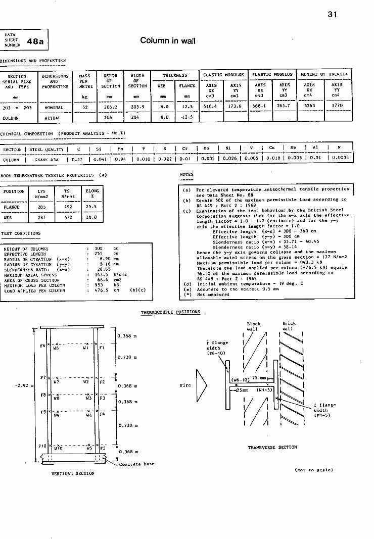
DATA SHEET 48 NUMBER

DIMENSIONS AND PROPERTIES

Column in wall

31

SECTION SERIAL SIZE

DIMENSIONS AND

MASS PER

DEPTH OF

WIiYIH OF

THICKNESS ELASTIC MODULUS PLASTIC MODULUS MOMENT OF. INERTIA

AND TYPE PKOPERT'ES METRE SECTION SECTION WEB FLANGE AXIS AXIS AXIS AXIS AXIS AXIS XX YY XX YY XX YY

mm kg m mm mm mm cm3 cm3 cm3 cm3 cm4 cm4

203 x 203 NOMINAL 52 206.2 203.9 8.0 12.5 510.4 173.6 568.1 263.7 5263 1770

COLUMN ACTUAL 206 204 8.0 .12.5

CHEMICAL COMPOSITION (PRODUCT ANALYSIS - Wt.%)

SECTION STEEL QUALITY C Si I Mn I P S I Cr Mo j Ni I V j Cu I Nb I Al I N

----------------

COLUMN I GRADE 43A 1 0.27 0.041 1 0.94 1 0.010 1 0.022 1 0.01 10.005 I 0.0261 0.005 I 0.018 10.005 1 0.01 1 0.0033

ROOM TEMPERATURE TENSILE PROPERTIES (a)

NOTES

For elevated temperature anisothermal tensile properties see Data Sheet No. 88 Equals 50% of the maximum permissible load according to BS 449 : Part 2 : 1969 Examination of the test behaviour by the British Steel Corporation suggests that for the x-x axis the effective length factor - 1.0 - 1.2 (estimate) and for the y-y axis the effective length factor 1.0

Effective length (x-x) 300 - 360 cm Effective length (y-y) = 300 cm Slenderness ratio (x-x) = 33.71 - 40.45 Slenderness ratio (y-y) 58.14

Hence the y-y axis governs collapse and the maximum allowable axial stress on the gross section = 127 N/mm2 Maximum permissible load per column = 843.3 kN Therefore the load applied per column (476.5 kN) equals 56.5% of the maximum permissible load according to 13S 449 Part 2 1969 Initial ambient temperature = 19 deg. C Accurate to the nearest 0.5 mm

() Not measured

THERMOCOUPLE POSITIONS

Block Brick wall wall

0.368 m

width W6 Wi Fl F65 - I flange

0.730 m (F610)

Fix- W7 W2 F2 (W6- 10)' 25 mm

2.92 mm (WI-5)

F9 * - - ------- 4 - -

F8 - x- - - - - - - - - -x -- - - 0.368 m

Fire

W8 W3 F3 0.368 m

I flange width

F W9 W4 (F 1-5)

0.730 m i A

F1O'l ------- I IF 1 TRANSVERSE SECTION

0.368 m

Concrete base

VERTICAL SECTION (Not to scale)

.0 I- z Di z

cc -12.5

25.0

12.5

£ C -, 0.0

a-

Q

-25.0

-37.5

-50.0

32 TEST CENTRE FIRTO -- BOREHAMWOOI) TEST DATE 3rd. NOVEMBER 1981 TEST NUMBER TE 4081

BS 476 PART 8 : 1972 ASSESSMENT

RE-LOAD TEST : SATISFIED STABILITY : 104 MINUTES INTEGRITY : 104 MINUTES INSULATION : 104 MINUTES FIRE RESISTANCE : 104 MINUTES

I DATA I SHEET 48b NUMBER

THERMOCOUPLE TEMPERATURE Deg. C AFTER VARIOUS TIMES (MINUTES) LOCATION

5 10 -------------

20 25 30 40 45 50 --

55 60 65 70 75 80 85 90 95 100 103 104

UNEXPOSED Fl 33 56 92 112 129 161 176 190 202 213 228 241 254 267 279 290 300 313 322 * FIANCE F2 19 34 60 75 95 136 155 172 186 199 217 234 246 258 269 279 288 298 304 *

P3 18 21 41 53 69 105 122 138 151 163 174 166 195 204 213 220 226 232 234 * F4 Il 19 34 46 60 92 108 123 137 148 162 176 187 197 207 215 223 230 233 *

- F5 16 17 23 28 36 54 63 71 78 86 95 104 112 120 127 134 140 146 149 *

MEAN 21 29 50 63 78 110 125 139 151 162 175 188 199 209 219 228 235 244 248

UNEXPOSED WI 37 66 125 150 174 220 241 259 276 292 309 326 340 354 367 379 391 403 411 * WEB W2 27 54 118 154 190 250 274 295 314 332 358 378 393 409 424 437 450 464 474 *

W3 20 33 82 115 144 190 210 228 244 259 277 295 307 320 331 341 350 358 364 * W4 20 32 76 106 132 178 199 220 236 251 278 300 315 330 343 355 366 376 382 * W5 18 23 43 61 80 112 125 137 148 158 169 181 191 200 209 218 226 234 238 *

MEAN 24 42 89 117 144 190 210 228 244 258 278 296 309 323 335 346 357 367 374

EXPOSED W6 121 217 400 478 542 639 670 700 733 765 797 824 843 861 881 899 915 931 940 * WEB Wi 101 210 431 535 615 707 747 786 818 845 874 892 906 920 937 952 964 977 983 *

W8 94 213 437 537 607 687 722 758 792 821 853 870 883 899 919 935 .948 960 966 * W9 74 170 385 486 559 653 694 731 762 791 831 853 867 886 909 926 939 952 958 * W10 51 100 250 365 454 550 584 615 642 671 713 748 768 790 816 840 860 887 882 *

MEAN 88 182 381 480 555 647 683 718 749 779 814 837 853 871 892 910 925 941 946

EXPOSED F6 155 283 513 604 668 743 772 804 836 862 887 902 914 928 944 957 970 983 989 * FLANGE F7 133 284 559 665 727 801 838 866 889 908 933 944 953 966 981 993 1004 1014 1018 *

P8 158 319 570 660 716 777 812 847 873 894 918 927 936 950 968 982 994 1005 1010 * F9 148 290 563 664 723 787 821 852 875 896 922 931 939 954 974 989 999 1010 1013 * PlO 90 172 415 584 677 739 764 790 815 838 874 893 904 919 939 957 969 981 980 *

MEAN 137 270 524 635 702 769 801 832 858 880 907 919 929 943 961 976 987 9991002

MEAN FURNACE GAS 589 657 808 825 856 882 896 913 927 940 955 963 970 988 1001 1014 1024 1035 1033 *

STANDARD CURVE (ci) 575 677 780 814 841 884 901 917 931 944 956 967 978 987 996 1005 1013 1021 1025 1027

DEFLECTION (mm) 6.5 16.7 21.5 8.4 -1.9-13.9-16.2-17.3-18.1-19.7-22.4-25.5-28.130.9-34.&-37.8-39.645.O * *

EXTENSION (mm)(e) 1.0 3.1 5.0 3.7 2.3 1.4 1.3 1.4 1.5 I.? 1.9 2.0 2.0 2.1 2.1 2.1 2.0 2.0 1.8 1.5

33

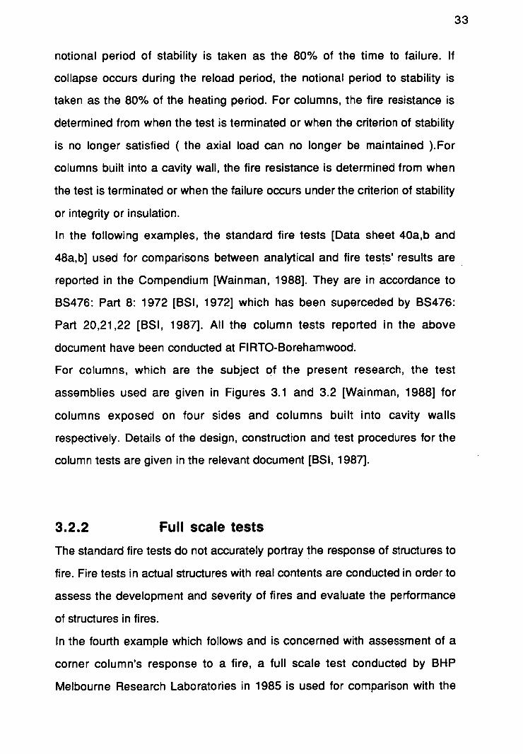
notional period of stability is taken as the 80% of the time to failure. If

collapse occurs during the reload period, the notional period to stability is

taken as the 80% of the heating period. For columns, the fire resistance is

determined from when the test is terminated or when the criterion of stability

is no longer satisfied (the axial load can no longer be maintained ).For

columns built into a cavity wall, the fire resistance is determined from when

the test is terminated or when the failure occurs under the criterion of stability

or integrity or insulation.

In the following examples, the standard fire tests [Data sheet 40a,b and

48a,b] used for comparisons between analytical and fire tests' results are

reported in the Compendium [Wainman, 1988]. They are in accordance to

BS476: Part 8:1972 [BSI, 1972] which has been superceded by BS476:

Part 20,21,22 [BSI, 1987]. All the column tests reported in the above

document have been conducted at FIRTO-Borehamwood.

For columns, which are the subject of the present research, the test

assemblies used are given in Figures 3.1 and 3.2 [Wainman, 1988] for

columns exposed on four sides and columns built into cavity walls

respectively. Details of the design, construction and test procedures for the

column tests are given in the relevant document [BSI, 1987].

3.2.2 Full scale tests

The standard fire tests do not accurately portray the response of structures to

fire. Fire tests in actual structures with real contents are conducted in order to

assess the development and severity of fires and evaluate the performance

of structures in fires.

In the fourth example which follows and is concerned with assessment of a

corner column's response to a fire, a full scale test conducted by BHP

Melbourne Research Laboratories in 1985 is used for comparison with the

Concrete cap

34

- -

II ,,,------r_i' I it —a— -

Steel end plate 406x406irunx19mm thick

If II

II

II II II

II

II

-. II

II

Steel column: 203 x203mmx

•1

52 kg/rn II

II

II

SI

II

II

II

If

II

If

II

II.

SI

II

Concrete base

II

Steel plates 406 x 406 mm x 19 mm thick

3.00 m exposec length

.64 m

Fig. 3.1 Vertical section of an unprotected column assembly (U.K.)

[Wainman, 1988].

iter

pos

Co

Ou

2flflmmkn/m Coiumn

vail

all

35

Brickwali

Ties

Fig 3.2 Configuration of a steel column built into a wall

[Wainman, 1988]

36

81

182 82 82

131

182 82 82

81 1— - -_ -

a00

, '0

.EVEL 3

£VEL 2

,ARPARI<

.EVEL 1

0 0 0

-J

5200

I- - - - -

ATRIUM

NON-LOAD BEARING COLUMNS 150 UC 23

i--i--

1--- -1 I I

OFFICE

OFFICE II I OFFICE t SED IN

EDGE OF SLAB

LAYOUT OF LEVEL 3

SULATED STEEL -- IALL PANEL (TESTS C1 -C)

SOUTH ELEVATION

PLAN - LEVEL 3

- 81 81

I B2 83 82 82 82

1-5% FALL -

I I

FALL -

FALL FALL

I

Bi

I I ID

I -N0N-L0AD BEARING COLUMNS 150 UC 23 (ESAIM =36 m 2 /ti

C C

B2 82 iB2 182 82

I r 5200 I 5200

FALL ON SLAB-LEVEL 1 ONLY

PLAN - LEVELS 1 & 2

Fig. 3.3 Building structural details - Plans and elevation

[Almand, 1989].

6 m NON - LAMINATED GLASS

PLASTIC SHEETING

12mm LAYER OF NON- FIRERATED PLASTER BOARD

(b) Facade for Test 02

Fig. 3.3 Building structural details - Office facade details

[Almand, 1989].

Unprotected steel

column

Hr bookcase\\F (chair

ir

H IL desk

filing cabinets air J

== = = I

facade rubbish bin

PVC covered chair

bookcase

lire protected, steel column

1 Hour fire

door

A

display board

desk extension

Fig. 3.4 Layout of office before test [Almand, 1989].

37

analytical results. The above mentioned full scale test was conducted in a

building consisting of a carpark above which there were an atrium and

several offices of which only one was used in the test. The actual office area

was 4m square in plan which is typical of a personal office space. Identical

protected and unprotected beam and column members were installed in the

office. A more detailed description of the building structure is given in the

Figure 3.3 [ Almand, 1989]. The office was furnished with typical contents i.e.

filing cabinets, chairs, bookcases, desks and paper (Table 3.1, Fig. 3.4). The

fire load is estimated to be 45 kg/m 2 wood equivalent which falls in the high

range of fire loads as surveyed in American office buildings [Almand, 1989].

The air temperature and steel temperature measurements in the office were

taken by thermocouples, the location of which are shown in Figures 3.5 and

3.6 respectively. Readings were taken at 50 seconds intervals. Even though

a sprinkler was installed in the office, it was not used at all. Observations

regarding the fire growth in the office are listed in the Table 3.2. Ventilation

was clearly the factor controlling the development of the fire in the test. The

maximum air temperatures recorded in the office throughout the test are

given in Graph 14. The maximum temperature was not always recorded in

the same location during the test. Graph 14 also presents a graphical

summary of the maximum cross sectional average temperatures for the bare

steel 150UC23 column in the office under consideration. No smoke

measurements were made during the test. However, it was observed that

significant quantities of smoke and flame exited from the window opening.

3.2.3 Existing Computer Programs

Most of the existing computer programs are based on two basic numerical

approaches, namely the finite difference and the finite element methods.

The finite difference approach directly models the differential equations

39

Table 3.1 Fire load in office [Almand, 1989].

Plastics 90 kg @ 40 MJ/kg = 3600 MJ

Paper 320 kg @ 17 MJ/kg = 5440 MJ

Timber 190 kg @ 17 MJ/kg = 3430 MJ

TOTAL 600 kg 12470 MJ

Wood equivalent @ 17 MJ/kg = 721 kg

Floor area =16rn2 (4mx4m)

Fire load =45 kg/M2 wood equivalent

40

A

-.7

- -J

• . 35.36.37.38 39.4-0.41.4.2

4.3, 4.4., 4.5,4.6

• . 4.74., 1.9, SO 51,52,53,S

PLAN

- 35,47 • 4. .

3 3951 - 36,48•4.4. 0410.52 - 1 37,49 0 1.5 04.1,53

38,504.6 04.2,54.

SECTION A-A

TEST 02

A

SUSPENDED CEILING

Other thermocouples: 68 and 69 on window, 300 and 700 mm below ceiling

Fig. 3.5 Air temperature thermocouple layout in office [Almand, 1989].

OTHER THERMOCOUPLES:

17,18, and 19 on north 150UC23 column in office, 1425 mm below ceiling 20,21, and 22 on north 150UC23 column in office, 300 mm above floor 23, 24, and 25 on north 150UC23 column in carpark, 300 mm below office floor

17 N

18

• 19(Typ)

26,27 and 28 on south 150UC23 column in office, 1425 mm below ceiling 29, 30 and 31 on south 150UC23 column in office, 300 mm above floor 32,33 and 34 on south 150UC23 column in carpark, 300 mm below office floor

F27YP Nj'

28

70 and 71 on bottom flange of beam in office ceiling space

I- - -

I - -

II

unprotected beam

1 proteted beam

(t9 ' ~20 00 Tio 12 9,1 0,11.12 I

000 1 5678

I ' 41,1615,16

1 --- - - - - -

41

Fig. 3.6 Steel temperature thermocouple layout [Almand, 1989].

42

Table 3.2 Observations of the full scale test in office [Almand, 1989].

TIME OBSERVATION (min.sec)

00.00 Ignition

00.40 Smoke rising, flames under desk

01.10 Flames above desk, no smoke visible outside office

Plastic film "window" moving in and out due wind

01.30 Door closed, window movement continues due to wind effects

07.40 Small hole ( approx 150 mm diameter) in plastic film, third panel from west, approx 200 mm above sill

Smoke visible outside office, emitted from top of west side window

16.10 Door opened to encourage more rapid development. Some flaming on floor

20.40 Fire visible above desk again, stacked plastic trays on desk burning

22.40 Flames building up on top of desk (plastic trays, etc)

24.10 Plastic film on windows distorting and disappearing, much greater smoke emission

24.40 Plastic curtains affected

25.10 East curtain disappears

25.20 West curtain disappears

25.30 Flames reach ceiling and spill out front of office

26.00 Flames spread to room divider

26.10 Glass windows above ceiling break

26.20 Flashover

27.10 Flames above ceiling

27.40 Smoke and flames emitted from top of door (between door and frame)

27.50 Ceiling panel falls (several have by this stage)

28.20 Full room involvement ceases

43

29—. 10 Ceiling panel tans (most nave corner chair continue burning

32.40 Rear bookcase also burning

44.40 Fire dies down, 2 small flaming areas

50.00 Door noted to be warped and door lock inoperative (not openable)

56.40 Door forced open (ash, etc behind door makes opening difficult)

describing the heat transfer for a particular problem. The finite element

approach discretizes the continuum.

Using finite element computer programs, one has to consider the trade-off

between computer size and mesh shape and size and the time increment

size. The smaller the mesh size and the time increment size, the larger the

required computer capacity. The choice of element size, shape and

orientation is a process of trial and error. The accuracy of the results is often

a function of the experience of the engineer using the model. The choice of

the time increment usually depends on numerical stability requirements.

Stability is a function of element boundary conditions, temperature

distribution and material properties.

There are two widely available finite element computer programs for

calculating heat transfer from fires to structures. These are described in the

following paragraphs.

TASEF - 2

TASEF (Temperature Analysis of Structures Exposed to Fire) is a thermo-

analysis computer program developed by Ulf Wickstrom in Sweden

[Sterner,1990]. It may be used to calculate temperatures in structures

exposed to fire. It is based on the finite element method. Although the

original version is limited to a two-dimensional analysis, the author states

that it could be modified to handle three dimensions. Structures comprised

of one or more materials can be analysed. At the boundaries, heat transfer

by convection and radiation can be modelled. Two dimensional rectangular

elements are used. Input of the geometry and generation of the finite

element mesh have been automated. Non-linearities due to temperature

dependence of material properties and boundary conditions can be

considered. Heat transfer by convection and radiation can be calculated.

45

TASEF-2 uses an explicit , forward difference time integration approach

which leads to shorter execution times and allows better modelling of latent

heat effects. It automatically calculates a critical time increment for each

iteration.

Details about the finite element approximation are given in the TASEF -

User's Manual [Sterner, 1990].

FIRES-

FIRES-T3 is a three-dimensional finite element computer program,

developed at the University of California, Berkeley. It is a very general

computer program which uses a backward difference time integration

approach. Because of that approach, latent heat effects in materials like

concrete or gypsum cannot be modelled directly. Instead, they are modelled

by assuming an appropriate internal heat generation. The backward

difference integration approach has the advantage of numeric stability.

If a small time increment is not initially specified, the program may reach the

point where it will not converge. The program must be restarted with a

smaller time increment.

Some typical input requirements of the program are listed below:

- Object geometry,

- Material properties as a function of temperature,

- Boundary conditions,

- Fixed temperature or a heat flux based on gas time-temperature data.

With both the above considered models, unecessary small time increments

can sometimes be avoided by assuming lumped temperature distributions. A

lumped temperature distribution assumes the same temperature for

adjoining nodes. In a similar manner, it is possible to assume a specified

temperature boundary condition instead of a highly non-linear heat flux

boundary. These approximations require a thorough understanding of the

physical basis of the heat transfer being modeled. Incorrect application of

these approximations may lead to serious errors.

Other ComDuter Proarams

ABA QUS

ABAQUS [Terro,1 987] is a computer program which is based on the finite

element method. It is developed to model solid body heat conduction with

general, temperature dependent conductivity, internal energy ( including

latent heat effects) and quite general convection and radiation boundary

conditions.

LUSAS

LUSAS [Terro,1987] is a finite element computer program. It is developed for

transient field analysis, governed by the quasi - harmonic field equation. The

finite difference discretisation in time employs the Crank - Nicholson rule:

9t+At = 2 O +M/2 - (3.13)

where: 0t = nodal temperature at time t

PA FEC

PAFEC [Terro,1987] is a computer program based on the finite element

method. It is developed for temperature analysis of complex engineering

structures. There are two choices of thermal calculation in this particular

program. It is the steady-state analysis and the transient-state analysis.

47

3.2.4 Existing Codes

ECCS [ECCS, 1983] recommends that the standard fire curve [BSI,1 987] be

used in calculations of the steel temperature. It is illustrated in Fig. 3.7 and

is given by the equation:

000 =345log 10 (8t+1 ). (3.14)

where: t=time;

furnace temperature at time t [°C],

00= furnace temperature at time t=O [°C].

The heat flow transmitted from the fire compartment to unit length of the steel

member is calculated using the following equation:

Q=KF(O - O.) [W/m] (3.15)

where:

Q =heat flow [WI m];

K =coefficient of total heat transfer [W / m 2 °C],

F =surface area of the member per unit length exposed to

heating [m2/m],

O t =ambient gas temperature at time t

0 =temperature of the steel member [°C].

The coefficient of total heat transfer has three components and is given by

the following equation:

K= 1 d

1 [WI m2°G]

(3.16)

cz + a. +

ki

where:

Otc = coefficient of heat transfer due to convection from the fire to the

exposed surface of the member [W/m 2 °C],

48

0 60 120 180 240

Time, min

Fig. 3.7 Furnace heating curve [ BSI, 1972 ].

Furnace temperature

c c

1200

1100

1000

900

800

700

600

500

400

300

200

100

49

a,. =coefficient of heat transfer due to radiation from the fire to the

exposed surface of the member [W /m 2 °C],

X i =thermal conductivity of the insulation material [W /m °C],

d =thickness of the insulation [m].

For bare steel elements, the equation of heat flow is given as follows:

Q= ( a + a. ) F 0)

where:

(3.17)

a=25

5.77e 8t273 O S + 273

-( 100 [W/m2°C]

where:

E = resultant emissivity of the flames, combustion gases and exposed

surface.

The value of a, given according to the equation, is based on experimental

investigations of standard fire exposure as well as natural fire exposure.

The value of ar is based on the Stefan - Boltzmann law.

The resultant emissivity c r depends on the type of the fire and the position of

the exposed member. EGGS recommends the value of 0.5 for the resultant

emissivity (Cr=05) which gives a conservative solution.

In Chapter Five (5) of this thesis, a more accurate evaluation of the resultant

emissivity is given according to the Swedish Fire Engineering Design of

Steel Structures [ Pettersson, 1976].

The calculation of the temperature increase Aq of a non- insulated member

exposed to fire is based on the assumption of quasi- stationary, one

dimensional heat transfer. The steel is considered as a heat sink, in which

50

the heat supplied is instantly distributed to give a uniform temperature. The

equation which describes the temperature increase of a member during a

time interval Dt is given as follows:

a AeS = (° - e5 ) At [°C] (3.18)

where:

a= a + a,. = coefficient of heat transfer [W /m2° C],

CS = specific heat of steel [J/ kg °C],

PS = density of steel [kg/m 3],

F =surface area of the member per unit length exposed to fire

[m2/m],

V =volume of the member per unit length [m 3/m]

O t =ambient gas temperature during the time interval At

[°CJ,

9$ =steel temperature during the time interval At [°C],

At =time interval [sec].

The temperature increase in the member depends on the geometry,

represented by "the section factor (F / V)' 1 .

The value of the time interval (At) , for convergence, has an upper limit given

below:

2.5 x104 FN [sec].

(3.19)

3.3 Examples

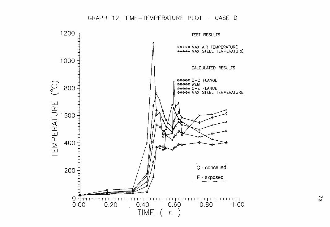
Four cases (Fig. 3.8) were analysed in order to assess the accuracy and

efficiency of TASEF-2. The solutions of the first case (column exposed from

four sides) and the third case ( column built into a wall) are compared to

temperatures measured during laboratory tests ( Data sheet 40a,b and

48a,b [Wainman, 1988] ). The solution of the second case (column built

next to a wall is compared relatively to the other two solutions because of

the lack of fire test results concerned with this particular problem. The

solution of the fourth case (corner column) is compared to temperature

measured during a full scale fire test in an office building [Almand, 1989].

The coefficient of convection heat transfer and the resultant emissivity of the

radiative mode of heat transfer have to be chosen. These factors depend on

the relative situation of the burners to the test specimens, the furnace size,

the type of fuel, the furnace wall characteristics. They are rather difficult to

be defined precisely. Values for the various factors have been chosen for the

four cases studied as listed below:

- Heat transfer by radiation

Estee l=O• 6

Cconcrete •• 0 • 8

where: c = resultant emissivity.

-Convective heat transfer

For the fire exposed surfaces,

=25.00 W/m 2K

r--1 .00

For the non fire exposed surfaces,

=2.25 W/m2K

r--1 .00

where: 3= convective heat transfer coefficient (W/m 2K),

= convective heat transfer power

51

52

The gas temperature obtained in the furnace should be identical to the

standard fire:

T=20+345 log 10 (8t+1 ) (3.20)

where: t=fire time in minutes.

The temperatures realised in the fire tests [Wainmann, 1988] are very close

to the ideal temperature curve so that all the tests can be classified as

standard fire tests. For the first and third cases, the temperature input for

TASEF-2 was taken to be the gas temperature as measured during the

actual fire test , used to validate the analytical results. For the second case,

the temperature input was taken to be the standard curve. The temperature

input for the fourth case was taken as the actual gas temperature measured

during the full scale test. Like most of the computer programs, TASEF-2 uses

as temperature input the gas temperature instead of the temperature of the

furnace walls. This gives a good approximation because of the low thermal

conductivity of the walls of the furnace.

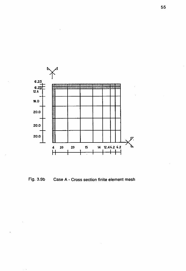
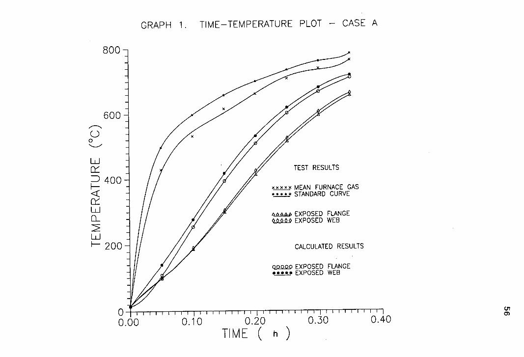
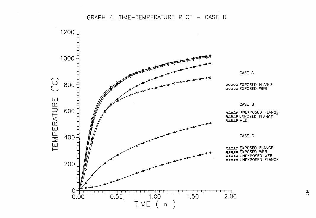
For each column studied, the cross section finite element mesh (Figs 3.9 -

3.12 ) used for analysis with TASEF-2 is illustrated. The results are

presented in the form of steel temperature - time plots (Graphs 1-14). The

measured and calculated results are in good concordance for the cases A

(Graphs 1-3) and C ( Graphs 7 -12 ). Case B ( Graphs 4 -6 )compared

relatively to cases A and C, shows good results. For Case D (Graph 12-14

), the measured and calculated results are in good agreement considering

the uncertainties involved in the simulation of a real fire environment.

The variation of the material properties of concrete and steel with temperature

was taken to be as given in the reference [Sterner, 1990].

51;1 Case C

53

: Ml) Case A

Case B

Case D

Fig. 3.8 Cases studied

<:

IFii. IFii.

54

Fig. 3.9a Case A - Cross section profile

IN 62

62± 12.6

18.0

20.0

20.0

20.0

ii

'.v

.'#

I:

Fig. 3.9b Case A - Cross section finite element mesh

55

GRAPH 1. TIME—TEMPERATURE PLOT - CASE A

0.10. 0.20 U.0 u.40

TIME(h)

0

u-i ry

400

ry Li 0 75 LU

200

[LIIS

oXiIi]

GRAPH 2. TIME-TEMPERATURE PLOT - CASE A

LiJ ry

400

ry

H-

u-i 0

LU H-200

0:10 0.20 0.30 0.40 TIME(h)

IIII]

ro.it (71

More

(3 0

GRAPH 3. TIME-TEMPERATURE PLOT - CASE A

[.1111

(3 0

Li ry

400

ry Li 0

LU 200

M

01 OD

0.10 0.20 0.30 0.40 TIME(h)

59

i•: ! ! ....

-- S;- PS ,e_ -

dt.1

I (...

MHOMM 1I I'

wo

FiT

Fig. 3.lOa Case B - Cross section profile

625 625

18.0

20.0

20.0

23.0

22.0

20.0

20.0

20.0

18.0

12.5

M.

6.25 III I I I Ii i' 12 20 20 4

Fig. 3.10b Case B - Cross section finite element mesh

[III

im

LU ry

ry

F-

LU 0

u-i F-

GRAPH 4. TIME-TEMPERATURE PLOT - CASE B

1200

1000

0C) 800

200

[ibiiJ 0.50 1.00 1.50 2.00 TIME(h)

CASE A

)oo EXPOSED FLANGE EXPOSED WEB

CASE B

UNEXPOSED FLANGE LO-0 EXPOSED FLANGE cxx WEB

CASE C

EXPOSED FLANGE Laus EXPOSED WEB

UNEXPOSED WEB i UNEXPOSED FLANGE

0)


0.50. 1.00 1.50 2.00 TIME(h)

U 0 800

LiJ ry

600

ry III

400

1200

1000

200

0) N.)

[1111]

rii.i.

LU ry

ry

F-

u-i 0

LU F-


1200

1000

00 800

0.50. 1.00 1.50 2.00

TIME(h)

C) (A)

CASE B

UNEXPOSED FLANGE LO-0 EXPOSED FLANGE , xx WEB

CASE C

EXPOSED FLANGE Lous EXPOSED WEB

UNEXPOSED WEB Lou* UNEXPOSED FLANGE

NO

Fig. 3.11 a Case C - Cross section profile

6.25

6.25 12.5 15.0

16.2 12.5

12.5 15.5

22.0

25.0

12.5 12.5 6.25 6.25

12.5

25.0

35.0

LuIu

65

1 50 50 30 30 1 18' 1 10104

Fig. 3.11 b Case C - Cross section finite element mesh

[;I.I

LU ry

ry

H-

u-i 0

Li H

GRAPH 7. TIME-TEMPERATURE PLOT - CASE C

1200

1000

0(3 800

ribI. 0.50 1.00 1.50 2.00 TIME(h)

0.

TEST RESULTS

is... MEAN FURNACE GAS 000 STANDARD CURVE

xx xxx UNEXPOSED FLANGE UNEXPOSED WEB

•...0 EXPOSED WEB EXPOSED FLANGE

CALCULATED RESULTS

00000 EXPOSED FLANGE 00 0 00 EXPOSED WEB AAA UNEXPOSED WEB OOO UNEXPOSED FLANGE


0.50. 1.00 1.50 2.00

TIME (h )

LiJ ry

600

ry III

400 Ld

1200

1000

800

200

0) -.4


0.50 1.00 1.50 2.00 TIME(h)

0C) 800

Li ry

600

Lij

400 LLJ

1200

1000

200


0.50. 1.00 1.50 2.00

TIME( h)

0C-) 800

Li ry

600

ry LLJ

400 Ld

1200

1000

200

m.


0.50 1.00 1.50 2.00

TIME( h)

U 0 800

u-i ry

600

ry III

400

1000

1200

200

0

Is

71

Fig. 3.12a Case 0 - Cross section profile

6.8

10

30

50

30

18.8

6.8

72

I I I I II 20 20 20 6.10

13.15 19.15 24 30

Fig. 3.12b Case D - Cross section finite element mesh

GRAPH 12. TIME—TEMPERATURE PLOT - CASE D

1200 TEST RESULTS

xxxx MAX AIR TEMPERATURE £AAAA MAX STEEL TEMPERATURE

CALCULATED RESULTS

0C-) 800

Lii ry

600

ry Li

400

00000 c-c FLANGE 00000 WEB

C—E FLANGE OOO MAX STEEL TEMPERATURE

200 C - conceiled

E - ex posed

-.4 CA)

0.20 0.40 0.60

0.80 1.00 TIME( h )

GRAPH 13. TIME-TEMPERATURE PLOT - CASE D

1200

1000

0(3 800

LU ry

600

ry Li

400

200

-.4

bIi]

0.20 0.40 0.60 0.80 1.00

TIME(h)

GRAPH 14. TIME—TEMPERATURE PLOT - CASE D

1200

1000

OU 800

Li ft:

600

ry bi

400 Li

ZE

0.20 0.40 0.60 0.80 1.00

TIME (.h)

200

Cii

P4fl1 1111: Structural Problem

77

CHAPTER FOUR Mechanical properties

The mechanical properties of interest are yield strength, modulus of elasticity,

tensile strength, creep. All the properties are strongly influenced by

temperature.

4.1 Stress and Strain - Axial loading

4.1.1 Stress-Strain Diagram at room temperature.

To obtain a stress-strain diagram for a material, one usually has to conduct a

tensile test on a specimen of the material. One type of specimen commonly

used is the one given in Fig. 4.1. The cross-sectional area of the cylindrical

central portion of the specimen must be accurately determined and two gauge

marks must be inscribed on that portion at a distance Lo from each other.The

testing machine in which the test specimen is then placed, applies a concentric

load P. As the load P increases, the distance L between the two gauge marks

also increases (Fig. 4.2). The distance L is measured with a dial gauge and the

elongation is recorded for each value of P. Simultaneously a second dial gauge

is often used to measure the change in diameter of the specimen. For each pair

of readings of the load P and the elongation d, one can compute the stress by

dividing the load by the original cross sectional area and the strain by dividing

the elongation by the original length Lo. The stress strain diagram is then

obtained by plotting the strain as the abscissa and the stress as an ordinate.

One can divide the materials on the basis of their common characteristics from

the stress-strain diagrams into two broad categories; ductile materials and

brittle materials.

Ductile materials are characterized by their ability to yield under normal

temperature.

78

Fig. 4.1 Typical tensile - test specimen

(Beer, 1979).

L I -r

j

GU—cYR

e

Fig. 4.2

Test specimen subjected to

tensile load (Beer, 1979).

Fig. 4.3 Stress - strain diagram for a typical

brittle material (Beer, 1979 ).

79

Brittle materials are characterized by the fact that rupture occurs without any

noticeable prior change in the rate of elongation (Fig.4.3).

Structural steel belongs to the first category which has characteristics as

follows. As the specimen is subjected to an increasing load, its length increases

linearly and at a very slow rate - the initial portion of the stress- strain diagram is

a straight line with a steep slope (Fig.4.4). After the value of stress has been

reached,the specimen undergoes a large deformation with relatively small

increase in applied load. This material property is called strain-hardening and

does not characterize the whole range of ductile materials. For example,

aluminium behaves differently. When a certain maximum load has been

reached, the diameter of the portion begins to decrease due to local instability

( Fig.4.5a). This phenomenon is called necking. After necking, the specimen

keeps elongating further under lower loads until it finally ruptures ( Fig.4.5b).

The failure of ductile materials is due to shear.Under an axial load,the shearing

stresses are largest on surfaces forming an angle of 450 with the axial load.

The material behaves elastically when the strains caused by the application of

the load disappear when the load is removed. This happens when the actual

stress is less than the elastic limit of the material. For the case of structural steel

the elastic limit coincides with the propotional limit and the yield point. The

behaviour of a material is plastic when the strains do not disappear when the

load is removed. Plastic deformation depends on the maximum value reached

by stress and the time elapsed before the load is removed.The stress

dependent part of the plastic deformation is referred to as slip and the time

dependent-which is also influenced by the temperature-as creep.

In the elastic range, Hooke's Law applies and the deformation is given by the

equation e=a/E. For multiaxial loading, the corresponding components of strain

are as follows:

60

MM a.0

40 UT

I ' U

20 1 ' I II II

YIeld Strain -hardening I4ccldng S it

0.02 0.2 0,25 0.0012

Low carbon steel

60. "U

40 - U'

20

0.001

Aluminum alloy

Fig. 4.4

Stress - strain diagrams of two typical

ductile materials (Beer, 1979).

() (b)

Fig. 4.5 Test specimen (necking - rupture) (Beer, 1979)

81

x- ' : E E

Cy= E E

-vax v(yz C E E

where: E = the modulus of elasticity of the material

V = the Poisson's ratio

(4.1)

The modulus of elasticity represents the ability of a material to resist

deformation, in other words its stiffness. It is expressed in the same units as

stress. BS 5950: Part 1: 1985 recommends the value of E=205 kN/mm 2 for the

design of structural steel at room temperature.

The Poisson's ratio is defined as the absolute value of the ratio of the lateral

strain over the axial strain and it quantifies the phenomenon that when a body is

pulled, it becomes longer and thinner or when compressed,shorter and thicker.

In the literature, most of the given values are derived from the relationship:

E V2G1 (4.2)

where E = modulus of elasticity,

G= modulus of rigidity.

1[Cooke, 1988] According to Woolman and Mottram, the values of Poisson's ratio derived from

the above equation are subject to considerable errors. The same authors

suggest that the best estimate for the family of low alloy steels - structural steel

is one of its members - are all between 0.27 and 0.30. BS 5950: Part 1: 1985 -

Structural Use of Steelwork in Building - recommends the value of v=0.30 for

room temperature design.

82

4.1.2 Stress-Strain Diagram at high temperatures

Modulus of Elasticity

4.1.2.1 Effect of temperature on flow stress elastic.

Stresses above the timit appearing due to the effect of a time variable

temperature field on the metal, cause residual deformations and strain

hardening, which subsequently can be combined by softening. The temperature

at which load is applied can also cause phase transformations and other

changes in the metal which can differ from those taking place in the metal under

constant conditions of heating (without stresses). These transformations under

the simultaneous effect of high temperatures and long-acting stresses may

cause unpredictable changes in the properties of the metal and impair its value

as a structural material. Temperature directly affects the mechanism of

resistance to plastic deformation and fracture. As the temperature increases, the

existing obstacles to dislocation movement become less effective and

dislocations can move in a crystal under appreciably lower forces, assuming

that the plastic deformation of the crystals occured by slip - twinning

deformation is observed at relatively low temperatures.

Slip is the displacement of a portion of a crystal relative to another portion while

the crystal structure of both portions remains unchanged. The boundary

between the portion where slip has occured and another portion where it has

not is called the dislocation line and is responsible for distortions in the

geometric regularity of arrangement of atoms in the original material. A

dislocation disappears after slip has been completed and a unit shear has

occured in a crystal (Fig.4.6). The great obstacles to dislocation movement are

the internal distortions in crystals which can be obtained by mechanisms of

strengthening because the dislocation locking increases the strain resistance of

a metal. The effectiveness of the strengthening methods depend on

OR

Fig. 4.6 Plastic deformation by slip ( Bernstein, 1979).

a-undeformed state of a crystal;

b-elastically deformed;

c-elastically and plastically deformed;

d-plastically deformed in which slip has taken place;

AB-slip plane.

••o• .+.w. .:.w. •.

••o, ..w. Ot•

•4• .eô.. .o'. •A4&S

.1... .o'o.

•p•• •.4 p.•+• .... ...o...• '•PA• •4O*

•.x.;.

..4. ....

.eis

..

.pi.. s:....

z••

...

Fig. 4.7 Climb of dislocations from one slip plane to another as a result

of self - diffusion and elevated mobility of vacancies at high

temperatures; the mobility of atoms in the lattice determines the

possibility of dislocation movement in a new slip plane (new

position) ( Bernstein, 1979 ).

1 - 5 stages of climb.

83

84

temperature. At an increase in temperature, movement of point defects is

activated appreciably and dislocation configurations can be changed by the

climb mechanism (Fig.4.7). Finally, an increase in temperature can cause

recrystalization which diminishes sharply the dislocation density and produces

softening.

4.1.2.2 Testing Methods

There are test methods to determine the ability of a material to withstand

external loads at elevated temperatures. It is possible to distinguish between

two main methods of testing:

- Static methods

- Dynamic methods

4.1.2.2.1 Static methods

The determination of the mechanical properties of metals in tests under static

loading is the most popular method. For determination of the stress - strain

diagram at elevated temperature, one is interested in the variation of flow stress

of a steel sample as a function of temperature. Regarding this, one may

distinguish between tests under transient heating conditions and steady-state

heating conditions. The three main test parameters are the heating process,

application and control of the load and control of the strain.

- Tests under steady-state heating conditions

Steady state is characterized by the steady state temperature curve as shown in

Figure 4.8.

The strain measured before the load is applied corresponds to the thermal

expansion. Four practical regimes can be used to determine the mechanical

properties.

-stress-strain relationship (stress rate controlled)

Failure

I • -J-"--Time H ts

zo.c

Time

ttH 1' S

Fig. 4.8 Typical steady state temperature curve (Anderberg, 1983).

t =heating period

ts =stabilizing period

=loading period (1-3 minutes).

ci) Load

Fig. 4.9 Stress rate controlled —E tests (Anderberg, 1983).

Loading procedure

Typical results

85

-stress-strain relationship (strain rate controlled)

-creep

-relaxation

aJ Stress rate controlled "a-c" tests are characterized by the loading

procedure as shown in Figure 4.9a.

The test may be used to provide the following data

-Compressive-tensile strength

-Modulus of elasticity

-Ultimate strain at collapse

Typical results of the above tests are given in Fig. 4.9b.

The stress-strain relationship is obtained in a high rate of loading -loading time

1-2 minutes- in order to avoid influence of creep which is significant for

temperatures above 400°C for ordinary steel. Under the influence of creep the

"a-c" curve is displaced in a way that we can notice a lower ultimate strength.

b/ Strain rate controlled "a-c" tests are characterized by the deformation

procedure as shown in Figure 4.10a.

The test can be used to provide the following data:

-Compressive-tensile strength

-Modulus of elasticity

-Ultimate strain at collapse

-Mechanical dissipation energy

The ultimate strain is related to the maximum stress level and not to the failure

state. For a given strain, a maximum stress is reached For higher strains, the

stress decreases somewhat but failure occurs at much higher strains than in

the corresponding stress controlled "a-c" tests.

Typical results are of similar nature to those of the stress rate controlled "a-c"

tests and are given in the Figure 4.1Ob.

87

Deformation

Time tH . tS .t

b)

C .,.

Fig. 4.10 Strain-rate controlled —c tests (Anderberg, 1983).

Deformation procedure

Typical results

MIM

The test may be repeated at different temperatures in order to develop a family

of load-extension curves from which one can extract the required

strength-temperature data, examples of which are shown in Figures 4.17, 4.18.

C/ Creep tests are characterized by the following loading procedure as

shown in Figure 4.11 a.

When the specimen is loaded, the load remains constant during the whole test

period

Typical results are given in Figure 4.11 b.

The test period of interest is from 2 to 4 hours.

A typical creep curve is given in Figure 4.41 where three phases can b&

indicated in the creep process which are primary, secondary and tertiary.

Usually, the primary and secondary phases are studied.

Tests for creep are usually carried out on unnotched test pieces,cylindrical or

rectangular ( Fig.4.12). BS18 recommends a gauge length of 40mm to be

adopted. The shape of the end portions of the test pieces should match the

design of the extensometer for measuring deformations. Testing machines are

classified according to the type of loading mechanism as: a)machine with direct

loading by weights, b) lever-type machines with upper lever, c) lever-type

machines with lower lever, and d) double-lever machines. Figure 4.14 shows a

scheme of a lower-lever machine. Heaters used in creep testing should meet

the following requirements:

- the temperature of the test piece must be uniform along the whole gauge

length,

- the temperature must be constant during the test,

- the device must ensure reliable and continuous heating for a sufficiently long

time.

The allowable temperature difference along the gauge length of a test piece is

±2 to ±6°C depending on the gauge length and testing temperature.

tHltS 0 1 2 3

4 At

Load Load

a)

Time,h

Strain

b)

Time,h

Fig. 4.11 Creep tests (Anderberg, 1983).

Loading procedure

Typical results

instantaneous stress-related strain

I_ wrzzl 152

l6_Ii 76 .I

901

JO ISI 120 JO

g "60 o 116

100 190

IN

Fig. 4.12

Test pieces for hot tensile tests

(creep or long-term strength) (Bernstein, 1979 ).

A l

6 C d

Fig. 4.13 Typical loading diagrams in machines

for creep and long-term strength tests

(Bernstein, 1979)

91

The temperature is regulated by means of dilatometric temperature controllers

whose action is based on either variation of the length of a reference rod placed

into the heater or variations of the dimensions of the metallic muffle of the heater

proper.

The creep deformations can be determined by means of indicators. A sample is

shown in Figure 4.15 as well as high temperature extensometerS. A diagram of

an automatic optical recording of creep deformations is given in Figure 4.16

where a light beam from a light source 1 passing through the diaphragm 2 and

collecting lens 3 falls onto a mirror 4 attached to the test piece. The deflected

beam is directed by mirror 5 on to a drum 6 rotating at constant speed and

carrying photographic paper. The light beam records the time-elongation curve

on the drum.

d/ Relaxation tests are characterized by the strain history as shown in

Figure 4.19a.

When the specimen is loaded, the initial strain is kept constant and the

decrease in stress is measured during the whole strain history.

Typical results are given in Figure 4.19b.

The test period of interest is from 2 to 4 hours.

- Tests under transient heating conditions

In tensile tests under transient temperatures, the load of the specimen is

maintained constant while its temperature is increased at a given rate

(Fig-4-20). The load can be applied before heating or developed during heating

by restraint against thermal expansion. These two types of transient tests are

carried out with load and strain control respectively. In this way, we can

distinguish two testing regimes:

-total deformation, failure temperature (stress control)

-total forces, restraint forces (strain control)

a' Stress control

Fig. 4.14 Extenders of an indicator extensometer

(Bernstein, 1979).

g. 4.15 Schematic of a creep-testing machine

with lower level (Bernstein, 1979).

5\__ 4.16 Diagram of automatic optical recording

of creep deformations ( Bernstein, 1979 ).

93

UTS •.•.• .•..• Fig. 4.17 Elevated temperature strength properties

I of a typical BS 4360: Grade 43A structural '•... //.o% PS

steel derived from steady-state tests

j2.o PS .. •. (Swinden Laboratories) (Kirby, 1988). -. .....-

'1 — — --- - - N

i.o% PS (BsI49) Maximum design stress

5 N/mm2

We 200 1400 600 800

Temperature, °C

Fig. 4.18 Elevated temperature strength properties of

a typical BS 4360: Grade 50B structural steel derived from

.. UTS

steady-state tests (Swinden Laboratories) (Kirby, 1988).

(s449) Maximum design stres in tension, 230 N/mm

0 200 400 600 800

Temperature, 0

C

b) CTI

0 1 2 3

Strain .1.. Strain .1..

E0 (T3 )

11 C0 (T2 )

4

rime,h 0 1 2 3 .1'

tH t S

Stress

Time,h

Fig. 4.19 Relaxation tests (Anderberg, 1983).

Strain history

Typical results

95

Temperature, 'C

T3

1 1 dt

ti t2 t3 .1

Time

Fig. 4.20 Typical transient state temperature curve

(Anderberg, 1983).

Load

(34

03

Gi

a) Time

11 1 2 t3 tL

Fig. 4.21 Transient tests with load control (Anderberg, 1983).

a. Load history

Temperature, 'C

a1

---

13 02

TI U4

I Oh- Ctotc1(I•/s

1 2 3 1. 5

I

20'C

((14 ) (03 )

C) I I I Temperature, 'C 11 12 13 14


b. Typical deformation curves

C. Typical strength-temperature relationships

.97

The load history of this test is given in Figure 4.21a.

A load is applied to the specimen before heating and then it is usually kept

constant throughout the whole test. The heating proceeds at a specified rate

within the range 5-50 0C/min until failure occurs.

Typical deformation curves are given in Figure 4.21 b.

The total deformation is recorded until the failure point where total strain

approaches infinity. The temperature measured at the critical points is called the

critical (failure) temperature. The results are very much influenced by the rate of

heating as creep cannot be avoided. With the aid of these curves, strength-

temperature relationships can be provided.

Typical strength-temperature relationships are given in Figure 4.21c.

If we extract thermal strain from the total deformation, one obtains "c-T" curves.

(Fig.4.22a,b). From these curves, one can construct "a-c" curves with creep

included. The heating rate has a great influence on "a-c" curves.

The specimen shape and the testing machine used do not differ from the ones

used under steady-state testing conditions described above, except that the

temperature provided by the furnace varies with time. An example of such a

machine is given in Figure 4.23. A similar one was used to provide elevated

temperature data on the behaviour of hot-rolled, structural steel for use in fire

engineering studies by British Steel Corporation at Swinden Laboratories.

The heater used is a three-zone, split furnace that was programmed to provide

constant specimen heating rates of 2.5, 5.0, 10, 20 OC/min which simulated the

average heating rates of fully loaded, steel sections surviving approximately 4,

2, 1 and 1/2 hours of fire exposure in the ISO 834 standard fire resistance test.

The load was transmitted to the specimens by means of Nimonic pull rods

passing through the ends of the furnace and hydraulically gripped in the

machine. Specimen strain was monitored by Nimonic extensometers fixed by

pressure screws at each end of the gauge length and measuring the elastic,

plastic srtains, as a result of the applied loads and thermal strain, due to thermal

Temperature

a)

T 31 T 1

2

I

2

ttotat••Eth E cr

Stress I I.

(13

0

11

'3

I +1 a. Cr


Typical E-T curves at four different stress levels

E =tot- Eth

Calculated —e curves (including creep) at

different temperatures

we

11

9

Fig. 4.23 a. Test piece, gauge length I = 75 mm,

diameter d = 4.5 mm.

b. General arrangement of test rig; 1. weights,

2.system of levers; 3. furnace; 4. test piece with

thermocouples, 5. temperature recorder; 6. dial

gauges.

(Thor, 1983)

•100

expansion. Separate tests were carried out under zero applied load to

measure the thermal strain separately and eliminate it from the results. When a

strain of 5% - regarded as the upper limit for practical use of flow stress data - is

the one when attained most tests were terminated.

For each steel and heating rate, a series of strain-temperature curves as well as

elevated temperature proof stress/room temperature yield stress-temperature

curves may be obtained (Fig.4.24).

b/ Strain control

In a strain control transient test, restraint forces arise. In Figure 4.25, the strain

history as well as typical curves of restraint forces are given. At temperatures

above about 550-600°C, the total force is independent of the initial load which

can be zero. If the total load minus the initial load is considered one will obtain

differing curves depending on the varying influence of creep.

This kind of test can only be carried out on steel members in compression with

no buckling influence (very short columns).

- Discussion

In international literature, there is little agreement amongst the elevated•

temperature elastic modulus data for steel grades within the family of structural

steels (Fig.4.26). The reasons vary and are related to testing machines, test

specimens, testing procedure, results interpretation.

Different tensile test machines have different accuracies measuring very small

strains and achieving a uniform and accurately known temperature over the

entire gauge length. This inaccuracy of strain measurements affects the stress-

strain curve to be affected and consequently the slope of the tangent at its origin

which is the modulus of elasticity.

'4' 1.0

' a02 - ' a

a20

S. 1.0

••55 a50 5%

S. .5.

S.

V V

S. S.

).6

\

\ \'

).4

\\ \\

-S. --

00 200 40O 600 Boo

Temperature (°C)

Fig. 4.24 a02, a 1 0.a20. a50 versus temperature for BS 4360: Grades

43A and 50B structural steels determined from tensile tests

conducted under transient heating conditions (Swinden

Laboratories) (Kirby, 1988 ).

101

1000

102

The chemical composition of the test specimens can affect the strain

measurements. For instance, larger plastic strains are measured with the

addition of small amounts of aluminium to improve notch toughness.

For anisothermal testing, one must be careful with the interpretation of the test

results. Deducting the thermal strain from the measured strain before plotting

the stress-strain curve results in higher derived elastic modulus values.

For isothermal testing, at high temperatures, the soaking period prior to

application of stress can relieve residual stresses causing grains elongated in

the hot-rolling process to return to their original shape. This could result in

shrinkage, and as a result the measured strain in a tensile test is reduced. In

isothermal testing, different rates of strain cause different values of measured

stress. A fast rate of strain results in higher measured stresses than a slow rate.

In Britain, according to BS 3688: Part 1:1963, which deals with tensile testing,

the rate of strain must be within the range of 0.001-0.003 per minute near the

elastic limit.

For structures in which the temperature is constant and the stress

fluctuates,isothermal data must be used. In building structures subjected to fire,

anisothermal data can be used assuming that the applied load is constant, as

on a floor above the fire, while the temperature varies. For structures where the

load and temperature vary, it is not clear which data should be used.

ECCS recommendation states that for stresses a—*0 , the modulus of elasticity

decreases with temperature and may - for all grades of steel and for the

temperature range 0:5056000C.- be approximated by the following equation

Eto 7.2x1 0 12O 4+11.8A 090334.5x1 070 2+1 5.9x1 )[N/mm2]

103

For temperatures over 600°C, the modulus of elasticity is not defined due to the

effect of creep which becomes more important and must be analysed explicitly

for such temperatures (Fig.4.27).

Arbed - the Luxembourg steel company - reported another relation between

elastic modulus versus temperature (Fig.4.25) which is given by the following

equations:

for 0!~

E

1 00°; E ° 00_i (4.3)

0 20 E

for 100°<0~600°C; E 08 0018( 0 )2 +0.036j+0.982

o 20

for 600°<0:5i 200°C 0 = 9.25926x1 0( -i-0.01 25() 2 0.34( j )+2.12

0 20 E

1 200°C<0; E ° 20

The variation of the plastic modulus E* with temperature reported by the same

company is given below:

E* for 0:5300°C; E

00 =5x1 0 -10+10-2

° 20 E*

for 3000<e!5600°C; E °0 --7x1 0 50+4.6x1 0 -2 (4.4) 0 20

E* for 600°C<0; E

00 04 10 2 o 20

The above relationships are used in a finite element computer program called

CEFICOSS (Computer Engineering of the Fire resistance for COmposite and

Steel Structures). Creep is not taken into account in an explicit way but implicitly

Strain

104

0)

E 04

03

((1 2

Ea

Temperature C

Total force

F4

F3 F2

F1 Temperature,C

300 600

Fig. 4.25 Transient tests with strain control (Anderberg, 1983).

Strain history

Typical curves of restraint forces

2.6

L)

c'J E E

1.6

(I)

1.0 t3 0

E

o os 4., Cl)

IM

I EMS 2 BSC .nljotjiermsl 1 BSC IsthtmeI 4 Ai-bed 6 Euronorm

6

4 3 2 4

0 200 400 600 000 1000

Steel temperature °C

Fig. 4.26

Variation of elastic modulus with

temperature (Cooke, 1987).

xi 0

E 6

in

N/mm2 2.0

1.5

1.0

0.5

0 200 400 600 800 1000


Fig. 4.27 Modulus of elasticity E t. as function

of the steel temperature (

ECCS, 1983).

105

106

by means of softened stress related strain. This happens due to lack of data and

because it is considered as a phenomenon of non-importance in real structures.

ECCS recommends an elastic modulus-temperature relationship given in

Figure 4.28.

The curve in Figure 4.26 has been developed from G.M.E. C000ke who

averaged the results that have been taken from an international survey made in

1980 from Stirland C., British Steel Corporation Teesside Laboratories which

included dynamically and statically derived data for different grades of

Euronorm 25-1972 structural steel. Kirby, SCI Sheffield Laboratories,

developed isothermal and anisothermal elastic modulus data. In the

anisothermal testing, steel grades 43A, 50B (BS 4360:1979) were tested, the

heating rates were 20,10,5,2.5 0C/mm, the applied stress-constant in each test/

varied from 15-250 N/mm2 for grade 43A and from 15-400 N/mm 2 for grade 50B

and the test terminated at 5% strain.

The anisothermal curves, developed by Kirby (1988), are given in Figures 4.28,

4.29.

4.1 .2.2.2 Dynamic methods

The dynamic methods are applicable at lower deformations where they possess

higher sensitivity than the static methods which present the risk that the test will

pass beyond the elastic region. In a dynamic test, the plastic and creep strains

are prevented from occuring due to the rapid stress reversal. This produces a

greater value for the modulus of elasticity than the statically derived one.

The specimen is usually a wire caused to vibrate. One end of the specimen is

usually held in a fixed clamp and the other oscillates freely across the path of a

light beam from a lamp to a photocell. The modulus of elasticity is determined

from the measured frequency of vibration at each temperature.

2.0

0.8

0.4 1m2

107

00 200 400 600 Boo

Temperature, °C

Fig. 4.28 Tensile curves for a Grade 43A steel derived

from transient tests ( Kirby, 1988).

108

1-0

C CU

C')

1.6

1.2

o.14

25 N/mm2

oc 200 1 00 600 800

Temperature, °C

Fig. 4.29 Tensile curves for a Grade 50B steel derived

from transient tests ( Kirby, 1988).

109

4.1.2.2.3 Suggestions

Generally, because the elastic modulus data can be produced with different test

methods, one must specify the test method used.

It is better for researchers concerned with structural analyses to adopt an E

versus temperature relationship which, though falling within the scatterband of

experimentally determined elastic modulus values, is chosen so that it best

correlates with bench-mark data.

4,2 Tensile Strength

The tensile strength can be defined as the ultimate tensile strength or the

tensile strength related to a specified residual stress induced strain in the

curve. It can be obtained either from steady state or transient state tests.

Parameters that influence significantly the analysis of tensile strength are given

below:

- in steady state tests

-rate of stress, a, at stress rate control

-rate of strain, c, at strain rate control

-in load controlled transient tests

-rate of temperature increase, T(°C/min),

-strain rate criteria

The influence of creep is different for each testing procedure.

It is shown that the relative strength decrease is almost the same for all hot-

rolled steels. The 0.2% proof stress and the ultimate strength of such steels

obtained in steady state and transient state tests have at 500-550 0C, 50% of its

original value left and at 700 0C about 20%.

4.3 Residual Stress

In hot-rolled steel sections important residual stresses may occur due to the

manufacturing process. These residual stresses may affect the structural

200 LOU ovu

uT

fu200c

I-c

0.

0.1

0. - 0

Temp,°C

110

Fig. 4.30 Residual properties (Anderberg, 1983).

a) Structural steel (j St 60/90, fu,20°c = 590 fiPa

c) Prestressing steel St 145/165, fu,200c 1650 MPa

OJ St 160.. .180, f ,20°C 1740 t4Pa

Test conditions tio loading during heating or cooling

Specimen hot-roiled, 0 = 26 mm

a Cold-drawn, 0 = 5.2 mm

GJCold-drawn, 0 = 5 mm

Chem. composition

Remarks : Residual ultimate tensile strength

Reference Dannenberg et al (1959)

III

Fig. 4.31 Residual properties (Anderberg, 1983).

a) Structural steel : ® St 60/90, f 0.2,20 °c = 590 MPa

C) Prestressing steel ® St 145/165, f 0.2,20 °c = 1520 MPa

(Jst 160...180, fO.2,20°C = 1570 MPa

Test conditions No loadinq during heating or coolinq

Specimen : (13 hot-rolled, 0 = 26 mm

(2)Cold-drawn, 0 = 5.2 mm

Cold-drawn, 0 = 5mm

Chem. composition

Remarks

Reference

T

0.220 0 C

1.0

0.6

OA

Residual 0.2% proof tensile stress

flannenberg et al (1959)

Temp, °C 04 0 200 £00 600

112

behaviour of fire-exposed columns. It is not yet known if the residual stresses

play an important role on the buckling load at elevated temperatures.

In some theoretical models, it is assumed by some workers that the residual

stresses vary as a function of the yield stress or that the residual stresses vanish

at elevated temperatures.

Experimental results presented in Figures 4.30, 4.31 show that the hot-rolled

steel is not influenced by temperature as it concerns neither the 0.2% proof

stress nor the tensile strength.

In the European Recommendations, it is assumed that the buckling curves at

elevated temperatures can be described by equations similar to those derived

for ambient temperature conditions.

4.4 Modelling steel behaviour

The deformation process of steel at transient high temperatures can be

described by three strain components:

(4.5)

where: eth(T) =thermal strain,

4 =instantaneous, stress related strain based on "a—c"

relationship,

Ccr(a,T,t) =creep strain or time dependent strain.

The deformation components are the same at steady state as well as at

transient conditions. The strains are found separately in different steady state

results.

113

4.4.1 Thermal strain

Thermal strain or thermal expansion is measured on unstressed specimens

under variable temperature and is given approximately by the following

equation, assuming linear relationship:

eh=Ja(T)dT (4.6)

where: a=coefficient of thermal expansion,

T=temperature (°C).

The linear relationship is most often used. The steel and strength characteristics

seem to have no significant influence. In a previous chapter ( Chapter Two ), a

discussion has already been given on the variation of thermal expansion with

temperature.

4.4.2 Instantaneous stress related strain

Many finite element programs require input of the stress-strain curves. In this

way, there is a real need to idealize these curves.

The experimental curve can be approximated in different ways.

The most straight forward way to model a stress-strain curve is to define the

yield strength by the offset method. The yield strength at 0.2% offset for

example is obtained by drawing through the point of the horizontal axis of

abscissa e=0.2%, a line parallel to the initial straight line portion of the stress-

strain diagram (Fig.4.32). The stress a corresponding to the point Y obtained

is defined as the yield strength at 0.2% offset.

Some other more sophisticated approximations of the stress-strain curve are

given in Figures 4.33,4.34.

aj

114

ire

C

Fig. 4.32 Determination of yield strength by

offset method (Beer, 1979).

Ily

4-40.2% offset

115

a

IT

IT

Ew

Fig. 4.33 Linear stress-strain curve models

£

a

116

2c

101

£

Fig. 4.34 Non-linear stress-strain curve models

117

[Anderberg, 1986] 1 The stress -strain model for steel using Ramberg -Osgood equation (1943)ii

given in the following table (Table 4.1):

Table 4.1

Temperature

range in °C

Yield stress aye Elastic Modulus E. no

80°C<O~200°C a x(0.978-O.034) y20 E20x[ 1-2. 8( 4 ) 2] 4600

0

200°C<0~400°C a x(O.978–O.O34) y20 E20x[1_2.8(52]

1485

2650

400°C<0~550°C a x( 1.553-0.1 55k) y20 E20x[ 1-2.8 (4)2} 0

2400

550°C<O~600°C a 20x(2.340-O.220) E20x(1-3 o020)21 1463

3900

0

6000C<O~690°C a 20x( 1 .374-0.078) E20x[ 1-3 .0(?4)2] 3600

o

690°C<O~800°C a20x( 1.120-0.1 28-k) E20x[ 1_3.0(?4)2] 4600

o

where: a= e

500 L( 1 . 50)

c= E

+ CF[2&] []5O 20 20

Cy E—+0.01 [1n8

E9

0--Temperature in °C (4.7)

for 20°C:50:!9800C (4.8)

for 800C<O:!98000C

[Anderberg, 1986] Magnusson (1974) modified Ramberg and Osgood expression as follows:

0 3 rO2T1 r 0 'ml Ca 7 -E(T)1 02T

(4.9)

where: 6:5m(T)!!-h50, m(T) = temperature dependent factor,

E(T)=modulus of elasticity,

f021=0.2% proof stress at temperature T.

118

[Anderberg, 19861 Dounas and Goirang (1982) developed the stress-strain relationship which

is described in Figure 4.33 The analytical expression for structural and

reinforcing steel is given below:

a=c0 E(T) 0!~Ca!~C i (4.10)

a=213+b\i 1-(2a—eja) 2 c 1 !5;c0:52a

2 (Ca 0•O3) a=b+ool23oo85T lecr

The parameters aj3,e 1 are dependent on temperature level and type of steel.

The analytical expression for reinforcing steel is different from the above.

Comments

Most of the existing finite element programs use bi-linear idealization. Making

idealizations is not an easy task especially if the elastic and plastic domains are

to be idealized bi-linearly. A bi-linear model is one that uses a straight line to

represent the elastic modulus and another to represent the plastic modulus.

Figure 4.33 shows two different bi-linear idealizations. The "a—c" model in

Figure 4.33a is appropriate for strains less than c% and will overestimate the

stress at higher strains. The "a—c" model in Figure 4.33b overestimates the

stress at the knee and it will require iterations if the load steps are not small. The

choice of a bi-linear curve is easier if the strain range is limited. Multinear

idealizations (

Fig. 4.33c) are easier to be made.


FRANSEEN [1987], author of CEFICOSS, uses a bi-linear model (Fig.4.33b) In

this particular model one can distinguish two linear parts, the slope of which can

be defined by the modulus of elasticity E0(T) and the plastic modulus E*(T)

respectively. Knowledge of the variation of the parameters Eo,E*,a provides

119

the definition of the relationship between a and ea for every temperature.The

same model had already been used in the program" Fires A-C" developed by

Bizri. During the early stages of his research, FRANSEEN had used the perfect

elastic-plastic model (broadly used at ambient temperatures), which did not

satisfied him and he comments in his research thesis that it is a very gross

model for the idealization of the "a—c" curve at elevated temperatures. He also

used a non-linear idealization in his program which he finally abandoned for

the following reasons:

-using the non-linear model, introduces difficulty in comparing the theoretical

curves with these resulting from testing and calibrating the parameters which

define the law.

-the numerical error using the bi-linear rather than non-linear is not so

important.

-the results from the analytical modelling as a whole do not present a

significant amelioration when the non-linear model is used.

FORSEN [Anderberg, 1976] in Steelfire - Finite Element program for Nonlinear

Analysis of Steel Frames exposed to Fire (1983) - uses a "a—c" curve

approximated by piecewise linear lines.

Codes

The European Recommendations for the Fire Safety of Steel Structures by

EGGS - Technical Committee 3 [ECCS, 1983] in order to apply elementary

plastic theory introduce the concept of effective yield stress. It is defined as the

level of stress for which the stress-strain curves are cut-off ( Fig.4.35 ) and it

decreases at increasing temperature.

For steel grade Fe360, the stress-strain curves are given in Fig. 4.36 assuming,

for practical purposes, that the heating rate does not significantly influence the

250

200

150

100

50

400

450

500

550

600

120 Cl) I C

actual behaviour l

4 I U) I

- CD

I >'

curve adopted in Cl) U) U)

U)

recommendations

ye .2? >' U) > () U) .4-

O.1e 0 0.5e 0 eye strain

Fig. 4.35 Simplification of the stress-strain curves

of steel at elevated tempeartures (ECCS, 1983). Stress

in N/mm2

0 0.1 0.2 0.3 0.4 0.5 0.6 Strain Ein%

Fig. 4.36 Stress-strain relationships at elevated

temperatures for steel grade Fe 360 ( ECCS, 1983).

121

deformation behaviour of steel structures under fire conditions - the creep is

included in an implicit way.

Stress-strain relationships for other grades of steel can be obtained through

recommented transformation based on the following assumptions:

a' For a given grade of steel the reduction in the effective yield stress at a

temperature O S is assumed to be the same as for Fe360. That means 9= YO~

for 0y20

all grades of steel. b/ For any grade of steel, the modulus of elasticity Ee at zero stress is assumed

to be equal to that of Fe360 throughout the temperature range.

The recommended transformation is illustrated in Figure 4.37 and the analytical

expression is given below:

a=a*+q ((;20235)

* ay20235 c=E +[p ]xlOO

tb

[N/mm2]

[N/mm2)

(4.11)

C

* C

E te

=actual stress

=stress parameter applying to Fe360

=temperature dependent coefficient

=nominal used stress of the used steel at room

temperature as specified in Euronorm 25-72

=effective yield stress of steel at elevated

temperature

=actual strain

=strain parameter applying to Fe360

=temperature dependent modulus of elasticity for a=O

where: a

a *

a (p= CT

y2O

G y2O

Oyo

stress a

in N/mm2

='(a 20 235)

[y2o235} 100 / ___

Aa

4 , I

L,e

curve applying to Fe360 for a certain temperature

transformed curve for

other grade of steel

I c1 strain cin%

Fig. 4.37 Transformation of the stress-strain curves for Fe 360 to other

grades of steel (schematic) (ECCS, 1983).

122

123

Tabulated values of the recommended stress-strain relations are given in the

ECCS Document for steel grades Fe31 0, Fe360, Fe430, Fe 510.

BS5950: Part 8 uses British Steel data which correlates better with the large

scale beam and column tests, both in terms of the heating rates experienced

and also the strains developed.

The British Steel data is consistent with a heating rate of 10 °C/minute. Similar

data can be obtained for other heating rates. It can be shown that the faster the

rate of heating, the higher the temperature at which a particular steel strength is

attained, for a given strain.

Full data is presented for strains up to 2% (Tables 4.2a,b). In BS 5950: Part 8,

Table 1 data is

only given for 0.5%,1.5%,2.0% strains because according to

experimental tests:

- a strain limit of 2.0% has been selected as being representative for the design

of composite members in bending protected with fire protection materials which

have demonstrated their ability to remain intact at this level of strain.

- a strain limit of 1.5% has been selected for the design of non-composite

members in bending which are unprotected or protected with fire protection

materials which have demonstrated their ability to remain intact.

- a strain limit of 0.5% applies for any other member (including columns).

The above strains should not be exceeded unless it has been demonstrated in

fire resistance tests that a higher level of strain can be satisfactorily developed

in the steel and that the fire protection material has the ability to remain intact.

British Steel data only covers the steel grades 43 and 50 complying With

BS4360. Data for cold finished steels complying with BS2989 is given in

Appendix B of the same document. Data for other grades of steel should be

established on the basis of elevated temperature tensile tests.

Table 4.2a Elevated temperature stress/strain data for BS4360: Grade 43A:1979 structural steels derived from transient tests (heating rate - 10 °C/min)

Strain 8

Stress in $/mm2 for Various Temperatures, Deg. C

20 50 100 150 200 250 300 350 400 150 500 550 600 650 700 750 800 850 900

0.00 0.0 . 0.0 0.0 0.0 0.0 0.0 0.0 0.0 0.0 0.0 0.0 0.0 0.0 0.0 0.0 0.0 0.0 * * 0.01 18.4 18.4 18.4 17.3 16.6 15.8 15.6 14.5 13.3 11.7 9.4 6.9 5.6 4.1 2.0 2.0 1.8 * * 0.02 36.7 36.7 35.7 34.9 33.2 31.9 31.4 29.1 26.8 23.5 19.1 13.5 11.5 8.2 4.1 3.8 3.3 0.03 55.1 54.1 54.1 53.3 49.7 47.7 46.9 43.3 40.0 35.2 28.6 20.4 17.1 12.2 6.1 5.9 5.6 * * 0.04 73.4 72.4 71.7 70.6 66.3 63.5 62.5 57.9 53.3 46.9 38.3 27.0 22.7 16.6 8.2 7.9 7.4 * 0.05 91.8 89.3 90.0 88.2 82.9 19.3 78.0 72.4 66.8 58.6 47.7 33.9 28.3 20.7 10.5 9.9 9.4 a

0.06 110.2 109.1 107.4 105.6 99.2 95.4 93.8 87.0 80.1 70.1 57.1 40.8 34.2 24.7 12.5 11.7 11.2 0.07 128.3 126.7 125.7 123.2 115.8 111.2 109.4 101.2 93.3 81.9 66.8 47.4 39.8 28.8 14.5 13.0 13.0 * 0.08 146.6 144.8 143.3 141.5 132.3 127.0 124.9 115.8 106.6 93.6 76.2 54.3 45.1 32.9 16.6 15.3 14.0 0.09 165.0 163.2 161.7 158.9 148.9 143.1 132.1 124.4 116.0 105.3 85.7 60.9 484 36.0 18.6 16.3 14.0 * 0.10 183.3 181.6 179.0 176.5 165.5 158.9 136.4 129.0 121.6 111.7 95.4 67.0 51.3 38.0 20.7 17.3 14.0 0.12 220.1 217.5 214.7 211.4 198.6 181.8 144.6 138.0 131.6 118.3 102.3 01.3 56.1 41.3 24.7 19.4 14.3 a a

0.14 255.0 247.1 234.1 225.4 208.1 188.2 152.2 145.9 139.5 124.7 108.6. 87.2 60.7 43.9 26.8 20.4 14.3 * S

0.16 255.0 247.1 238.4 229.5 213.4 193.8 158.9 152.2 145.9 130.8 113.5 92.6 64.3 46.2 28.1 21.4 14.5 * S

0.18 255.0 247.1 242.3 232.6 217.5 198.4 164.5 157.8 151.2 135.9 118.6 96.9 67.6 48.2 29.6 22.2 14.8 0.20 255.0 247.1 244.8 234.6 22..L...1 202.2 169.8 163.2 156.3 140.3 122.9 100.0 70.9 50.0 31.1 23.0 15.0 0.25 255.0 247.1 246.1 237.7 229.2 208.8 181.3 174.7 167.8 150.2 132.3 105.8 77.3 54.3 34.9 25.0 15.6 * * 0.30 255.0 217.1 246.1 239.7 233.8 213.9 191.8 184.9 177.7 150.9 140.3 110.7 02.9 58.4 38.3 27.0 16.1 • S

0.35 255.0 247.1 246.1 241.0 237.4 217.3 199.7 192.8 185.9 166.5 146.4 115.5 87.5 62.5 41.1 28.6 16.6 0.40 255.0 247.1 246.1 241.7 239.2 219.0 207.1 199.7 192.3 172.9 151.5 119.3 91.3 65.3 43.6 30.1 17.1 0.50 255.0 247.1 246.1 243.8 241.2 225.4 217.8 210.6 203.5 183.9 158.6 125.5 96.4 68.6 47.4 32.4 18.1 0.60 255.0 247.1 246.1 244.0 241.7 230.0 225.7 218.5 211.4 192.5 165.5 131.8 100.5 70.9 49.5 33.4 19.1 12.8 0.70 255.0 247.1 246.1 244.3 242.3 233.6 230.8 225.2 219.6 199.9 172.4 137.4 103.8 72.9 50.7 34.2 20.1 13.8 0.80 255.0 247.1 246.1 244.5 242.8 237.4 235.4 231.5 227.5 206.0 177.2 142.0 107.4 75.0 51.8 34.9 21.2 14.5 0.90 255.0 247.1 246.1 244.5 243.0 240.7 238.7 235.6 232.8 210.9 181.3 145.9 110.2 76.5 52.8 35.4 22.2 15.3 • 1.00 255.0 247.1 246.1 214.8 243.5 242.8 241.2 239.7 236.9 214.7 104.1 148.9 111.7 77.8 53.5 36.2 23.2 16.1 1.20 * a a a • 215.6 243.8 240.2 221.3 188.2 152.5 114.2 80.1 55.1 37.2 25.2 17.3 • 1.40 * a a a • 245.8 242.0 226.4 191.3 155.0 116.3. 82.1 56.1 38.3 27.0 18.4 11.0 1.60 a a a a a a a a 244.0 231.3 193.8 157.1 118.1 83.9 57.4 39.0 28.1 19.1 15.3 1.80 a a a a a a a a 246.3 235.4 196.1 158.6 119.6 85.2 58.4 39.0 28.8 19.9 15.6 2.00 a a a a a a a a * 238.2 197.9 159.9 120.9 85.9 59.2 40.3 29.3 20.1 15.8

No data.

r")

Table 4.2b Elevated temperature stress/strain data for BS4 360: Grade 50B :1979 structural steels derived from transient tests (heating rate - 10 °C/min

Stress in M/=2 for Various Temperatures, Deg. C strain

350 400 450 500 550 600 650 700 750 800 850 900

20 50 100 150 200 250 300

0.00 0.0 0.0 0.0 0.0 0.0 0.0 0.0 0.0 0.0 0.0 0.0 0.0 6.7

0.0 5.7

0.0 4.3

0.0 2.1

0.0 2.1

0.0 1.8

* *

0.01 18.8 18.8 18.8 17.8 16.3 15.6 15.6 14.6 13.1 26.6

11.7 23.4

9.6 18.8 13.5 11.4 8.2 4.3 3.9 3.9 a

a 0.02 37.6 37.6 36.6 35.9 33.0 31.6 31.2

46.5 28.8 43.3 39.8 35.1 28.4 20.2 17.0 12.4 6.0 6.0 •7

0.03 56.1 55.4 55.4 54.3 72.4

49.3 65.7

47.2 63.2 62.1 57.5 53.3 46.5 38.0 27.0 22.4 16.3 8.2 7.8 7.5

9.2 • 0.04 74.9

93.7 74.2 92.7

73.1 91.9 90.2 82.4 78.8 77.7 72.1 66.4 58.2 47.6 33.7 28.0 20.6

24.5 10.3 12.4

9.9 11.7 11.4 * a 0.05

0.06 112.5 111.5 109.7 107.9 98.7 94.8 93.4 86.6 79.5 69.9 81.7

56.8 66.4

40.5 47.2

33.7 39.4 28.8 14.2 13.8 13.1 • a

• a 0.07 131.0 129.2 128.5 125.7 115.0 110.4 109.0

124.3 100.8 115.4

93.0 106.1 93.4 76.0 54.0 45.1 32.7 16.3 15.6 14.9

a a 0.08 149.8 148.0 146.3 144.5

162.2 131.7 148.0

126.4 142.0 139.9 129.6 119.3 105.1 85.2 60.7 50.8 36.9 18.5 17.0

19.5 16.7 18.5 a a

0.09 0.10

168.6 187.4

166.9 185.7

165.1 182.8 180.3 164.4 158.0 155.1 143.8 132.4 116.4 94.8 67.4

80.9 56.4 66.0

40.8 49.0

20.6 24.5 22.0 19.9

0.12 224.7 222.2 219.4 215.8 197.4 189.6 183.2 171.1 159.0 177.9

139.5 158.0

113.6 132.8 94.4 74.2 53.6 28.8 24.3 19.9 • a

a a 0.14 262.3 259.5 256.0 252.4 230.4 221.2 198.8

211.6 188.5 201.6 191.3 170.0 145.2 107.9 81.7 58.2 33.0 26.6 20.2

a a 0.16 299.6 296.1 292.5 288.3 263.4

287.9 251.0 264.8 221.9 212.6 203.1 180.3 156.2 120.3 88.0 62.5 36.6 28.4 20.6

20.9 a a 0.18 337.3

355.0 333.7 343.1

328.4 333.7

313.8 318.8 300.7 273.0 231.8 222.2 213.0 188.5 165.8 130.6 94.1 66.0

74.5 39.8 46.2

30.2 33.7 21.7 a a

0.20 0.25 355.0 348.6 338.7 326.6 316.3 287.2 250.6 241.8 232.5 205.3

220.5 182.8 195.3

145.6 154.1

105.1 115.0 81.3 51.5 36.6 22.4 a a

• a 0.30 355.0 349.7 341.2 332.6 325.2 296.8 267.0

278.0 257.0 268.4

247.4 258.8 231.8 203.8 160.8 121.8 87.0 57.2 39.0 23.1

0.35 355.0 350.0 342.6 336.5 338.7

330.5 333.0

302.5 306.0 288.3 278.0 267.7 240.7 210.9 166.1 127.1 90.9 60.7 41.9

45.1 23.8 25.2 a a

0.40 355.0 355.0

350.0 350.4

344.0 345.4 340.8 335.8 313.8 303.2 293.2 283.3 256.0 220.8 174.7 134.2

139.9 95.5 98.7

66.0 68.9 46.5 26.6 17.8 a

0.50 0.60 355.0 350.4 345.8 341.2 336.5 320.2 314.2 304.2 294.3 268.0

278.3 230.4 240.0

103.5 191.3 144.5 101.5 70.6 47.6 28.0 19.2 a

0.70 355.0 350.7 346.1 341.9 337.3 325.2 321.3 313.5 305.7 316.7 286.8 246.7 197.7 149.5 104.4 72.1 48.6 29.5 20.2 a

a 0.80 355.0 350.7 346.5 342.2 338.0 330.5 327.7 322.3

328.0 324.1 293.6 252.4 203.1 153.4 106.5 73.5 49.3 30.9 21.3

0.90 355.0 350.7 346.8 342.6 338.3 335.1 332.3 335.8 333.7 329.8 298.9 256.3 207.3 155.5 108.3 74.5 50.4 32.3 22.4

24.1 a 1.00 355.0 351.1 347.2

a 343.3

* 339.0

a 338.0

• 341.9 339.4 334.4 308.1 262.0 212.3 159.0 111.5 76.7 51.8 35.1 37.6 25.6 20.6

1.20 a * a a * a 342.2 338.0 315.2 266.3 215.8 161.9 114.3 78.5 53.3

34.3 39.0 26.6 21.3 1.40 a.

a a a a a a 340.8 322.0 269.8 218.7 164.4 166.5

116.8 118.6

79.9 81.3 55.4 40.1 27.7 21.7

1.60 1.80 a a a a

* a *

a a

a a

a 342.9 a

327.7 331.6

273.0 275.5

220.8 222.6 168.3 119.6 82.4 56.1 40.8 20.0 22.0

2.00 a

*No data.

rs) (11

126

EGGS data [EGGS, 1983] is conservative relative to the anisothermal data

produced by British Steel. They use an effective yield strain of 0.5% for

temperatures above 400 0G even though in fire tests on beams and columns it

can be shown that much higher strains are experienced. For the above reason,

British Steel data replaced that of EGGS in the proposed Eurocode 3

[Eurocode No. 3, 1990].

The model for stress-strain relationships of steel at elevated temperatures in the

proposed Eurocode 3 is given in Figure 4.39.

where: Ea(e) slope of the linear elastic range of the stress-strain

relationship of steel in the fire situation.

Gam(0) effective yield stress of steel in the fire situation

cNapr(o) proportional limit of steel in the fire situation

strain corresponding to the effective yield stress of

steel in the fire situation

Capr(0) strain corresponding to the proportional limit of steel

in the fire situation

subscript a means steel

According to this proposed model and for heating rates 2-50°G/min, we can

distinguish three regions which are : elastic, non-linear, plastic ( Fig.4.38). The

stress-strain curves can be described by the slope of linear elastic range (Eaf) ,

the propotional limit (fy11 the effective yield stress (f f). The variation of the

characteristic values of these parameters related to their temperature values are

given in Figure 4.38.

The stress-strain relationships in British Standards and Eurocode 3 are based

on British Steel data which have been derived from small scale tensile tests.

These relationships may also be applied to steel in compression.

07

max(e)

018 \ pr(e) l

In N

\

i

'e Pr (9) it& Calm) U(0) amax(e) 12 %

Fig. 4.38 Mathematical model for stress-strain relationships of steel at

elevated temperatures (Eurocode 4, 1990).

Range

elastic E.,'

II \fa2_ (Ea max j , Eit)+crapro,_ 1

transit with

elliptical 8 2 = Irs(Ol (E1 max(e,Es prie,) 24 c(Eem.xorEa pqo)

b2 = E,..(E.m.xt.,E.pr(,))-C4c2

((i, m a x a C

2 (Or. pre,Uamizi.,) 4 r...,(E max(e 6 a puei)

plastic 0

Fig. 4.39 Definition of the various parameters of the mathematical model

of figure 4.38 ( Eurocode 4, 1990 ).

127

128

4.4.3 CREEP STRAIN

The models by which the mechanical properties of steel at elevated

temperatures are described can basically be distinguished in sophisticated and

pragmatic models. Sophisticated models include creep explicitly. Pragmatic

models present the strength and deformation properties by a set of

temperature-dependent stress-strain relationships and creep is included in an

implicit way.

Models of creep are in most cases based on the theory put forward by Dorn

(1954)[Thor, 1973] which permits consideration of the variation of temperature

with time.

The creep strain to be modelled here is based on Darn's theory - i.e it is

dependent on the magnitude of the stress and on the temperature-

compensated time given by the following relation:

t

(-LH

O=Jefdt(t) (4.12) 0

where: AH=activation energy required for creep (cal/mol),

R=universal gas constant (cal/mol K),

T=temperature (K),

t=time (hours).

The relation between the creep strain c and the temperature-compensatedCr

time 0 (t), for different stresses a is shown in Figure 4.41. The curve expressing

this relation contains a portion of constant slope (decrldO=Z ) which is

dependent only on the magnitude of stress and defines the secondary phase of

creep. The primary phase is defined by a parabolic equation. The transfer from

the primary to the secondary phase occurs at time 0 0 .and the intersection

between the straight line and the creep strain axis is called Ecr

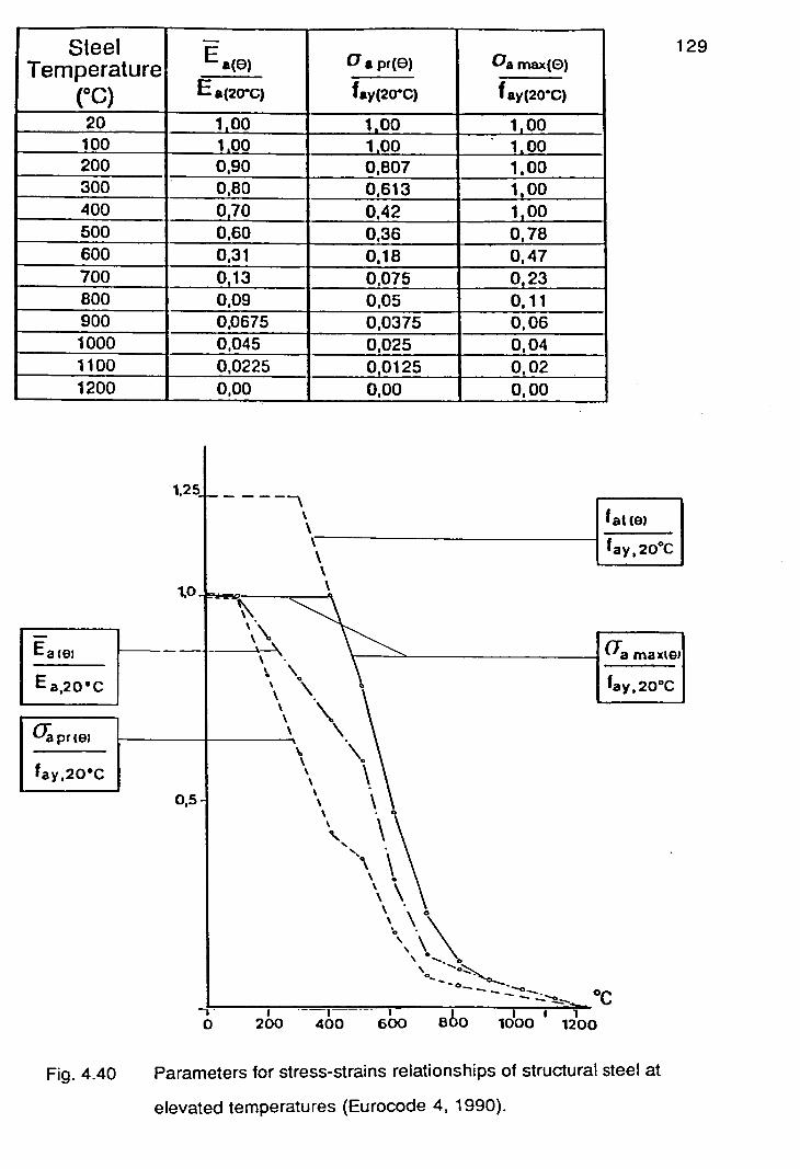
Steel Temperature

(°C) a(20C)

Cr a pr(s)

fsy(24rC)

0a max(0)

fay(20C)

20 1 1 00 1,00 1,00 100 1 100 1 100 1,00 200 0,90 0,807 1,00 300 0,80 0,613 1,00 400 0170 0,42 1,00 500 0,60 0,36 0,78 600 0,31 0,18 0,47 700 01 13 0,075 0,23 800 0,09 0,05 0,11 900 0,0675 0,0375 0,06 1000 0,045 0,025 0,04 1100 0,0225 0,0125 0,02 1200 0,00 0,00 0,00

Fig. 4.40 Parameters for stress-strains relationships of structural steel at

elevated temperatures (Eurocode 4, 1990).

129

130

Time

Secondary phase

4.41 Measured creep curve approximated by two straight branches

with slopes Z, Z5 (Anderberg, 1986 ).

0.22

G 601C

-7 O 220C • 0.29

'I / ,

II

I' ll II 'I

/ ,

1 ,

0.22

J

1. 0.15

.1 602C

0.15 .1- sae.c

0.5 1:0 Time, h

42 Measured and predicted creep (modification Dorn-Harmathy

theory) at different stress levels. Reinforcing steel K S

60 48,

fo.2200c710 MPa ( Anderberg,1983 )

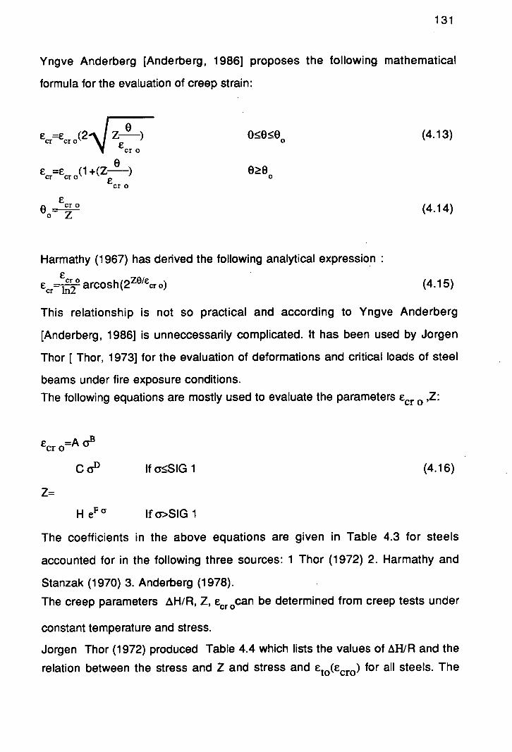
131

Yngve Anderberg [Anderberg, 1986] proposes the following mathematical

formula for the evaluation of creep strain:

eCr cro =c (2-' 0:050 (4.13) \/

Cr Cr0 0

C (4.14)

0- Z

Harmathy (1967) has derived the following analytical expression C

CTO LIZOIC C = arcosriv crin2

This relationship is not so practical and according to Yngve Anderberg

[Anderberg, 1986] is unneccessanly complicated. It has been used by Jorgen

Thor [Thor, 1973] for the evaluation of deformations and critical loads of steel

beams under fire exposure conditions.

The following equations are mostly used to evaluate the parameters ,Z:

Ccr 0=A cy

lfa:5SIG1

(4.16)

Z=

He F cy lfo>SIG1

The coefficients in the above equations are given in Table 4.3 for steels

accounted for in the following three sources: 1 Thor (1972) 2. Harmathy and

Stanzak (1970) 3. Anderberg (1978).

The creep parameters AH/R, Z, Ecrocan be determined from creep tests under

constant temperature and stress.

Jorgen Thor (1972) produced Table 4.4 which lists the values of WR and the

relation between the stress and Z and stress and Cto(Ccro) for all steels. The

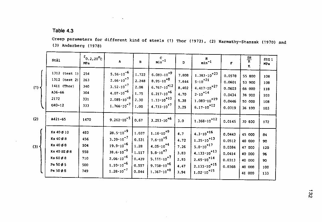
(1)

Table 4.3

Creep parameters for different kind of steels (1) Thor (1972), (2) Harmathy-Stanzak (1970) and (3) Anderberg (1978)

Stal f 0 o .2,20c

A B C

- 1 H . 1

SIG1 MPa mm D mm F MPa

K

1312 (test 1) 254 5.56.106 1.722 6.083.10 7.808 1.383.10+23 0.0578 55 800 108 1312 (test 2) 263 2.6610 2.248 8.95.10+8 7.644 5-10 +21 0.0601 53 900 108 1411 (Thor) 340 3.52.10 2.08 6.767.10+12 8.402 4.417.10+27 0.0603 66 000 118 A36-66 304 4.07.10_6 1.75 6.217.10+6 4.70 2.10+14 0.0434 38 900 103 2172 331 2.085.108 2.30 1.33.10+10 5.38 1.083.10+19 0.0446 50 000 108 G40-12 333 1.76610 1.00 4.733•10 3.25 6.17.10+12 0.0319 36 100 103

A421-65 1470 9.262•10 0.67 3.253.10+6 3.0 1.368.10+12 0.0145 30 600 172

Ks 40010 483 28.510 1.037 1.1610 4.7 4.3.10+16 0.0443 45 000 84 Ks 4008 456 3.39•10 0.531 7.610 4.72 1.25.10+13 0.0512 40 000 90 ICs4008 504 19.9.10_6 1.28 4.0510 7.26 0.0384 47 000 120 Ks 40 5E08 558 38.6'10 1.117 5.810 3.83 4.133.10+13 0.0414 40 000 96 I(s6008 710 2.06.106 0.439 5.1111O 2.93 2.65.10+14 0.0313 40 000 90 Ps 5005 500 1.10•10 6 0.557 9.738.10+6 447 2.133.10+15 0.0368 40 000 100 Ps5008 749 1.28•10 0.844 1.367.10+8 3.94 1.02.10+15 41 000 133

f (A)

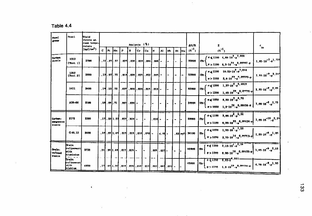
Table 4.4

Itee1 Reid

plow treaS at room tpvw. - - - - An1yaie (%) - - - - - MI/it z

(kgf/eirP) C SI Mn P S Cr Cu N Al Nb NI Mo (h ) (h )

carbon 1312 37.008

( 7çnoo 4,09.10 .o 2590 .11 .05 .57 .025 .0341 .020 .ons .ono - - - - 55600 1 f0r 1.0210 -7

.

1.72 0

(feat 1) 0 001417 10>1100 8,310 .e

2 7,644 1100 10,53.10 •o 1312 2) 2660 .1. .07 .75 .01(1 .025 .0 .052 .005 - - - -

$39" fllr{ 1.44.10t.2.2

-

23S005 a> 1100

- -

- (V10200 1,37.104.c4410 1411 $400 .1' .13 .73 .035 .020 .020 .015 .013 - 6000 fl3T( 2.@2-10-9-0

I 02 29 0 02•'12.

10>1200 1,45•10 . -• 0

( o.1050 e,so.io3. 4,70 A36-46 3100 .11 .09 .71 .007 .030 30900 tOrj

00429.0 L 0>1030 1,210 •e

- - - - - - -

--

- -

- ççiioo Con- 2172 3350 .11 .33 1.5 .022 020 - - .010 - - - - 50000 mn 1,00.1010.02.5

14sfleS• 20 0 00436 (o>1100 9,50•10 •e • .tis

41 2 23

c 1050 1,50.10

( • 040,12 3400 .1. .02 1.4 .015 .019 .010 .0410 .03 ,Ø 30100

14 0 0>1020 3,70•10 •e ' ,

rain l70 0 E 1300 2,1010 '0

retimd

efineeient 11th

3730 .21 .3(1 1.10 .017 .019 - - .005 .02: - - - 40900 tor{

10 0.00153.01.413-110-9.v 2.15

dials 3tri1niw 0> 13110 S. 00' 10 'e

rain a1250 efine,.!nt

.

13000 f0r 47010 9195 aith 4050 .17 .42 1.21 .010 .020 .015 .014 .007 • 00' .021 - - I.l25O 1,210 •e0' 34'0 iobitii,

(A) CA)

134

Table also gives the analyses of the various steels and their yield stresses at

room temperatures. One can notice from the same table that in some cases

large differences occur even when steels that belong to the same group are

compared. This is due to the yield stresses which vary even for steels in the

same group. Another reason is that the determination of AH/R is sometimes

sensitive and may therefore be subject to some inaccuracy. The values of AH/R

affect the magnitude of Z derived from the equation:

dE dEdt Z=(t )=( —)=e e'IT (4.17)

where: e=rates of creep during the secondary creep stages of the conventional

creep tests- creep tests at constant temperature and stress.

Since it is not the value of AH/R or Z in themselves but a combination of these,

some uncertainty in the value of iH/R can normally be accepted. It is shown that

that calculated creep strains at stresses which are the same in relation to the

yield stress of the steel concerned at room temperature shows good agreement

within the same principal group , in spite of differences in the values of AH/RT

and Z. The values of the above parameters are regarded not as exact material

data but rather as empirical values and relationships which when used in the

equations for the determination of temperature-compensated time and creep

strain produce creep curves which are in good agreement with those plotted on

the basis of tests.

Anderberg used the Harmathy expression to compare test results with analytical

results for reinforcing steel Ks 60 48.(Fig. 4.40).

A simplified way to approximate the curve which illustrates the relationship

between the creep strain and the temperature-compensated time, is given in

Fig.4.41 which contains two straight branches with slopes Z, and Z. The

analytical expression is given below:

135

ç(t,T,a)=t Z(T,a) (4.18)

E =Z (T,a) if 05t5t Cr p t

CCTZS(T,cN) if t>t E*

E (4.19) 20

Comments

ANDERBERG accepts a simplified model for creep [Anderberg, 1986] . He

comments that a simplified model where the creep strain is incorporated in the

stress-strain relationship in approximate way is appropriate for design purposes

but is not accurate enough for analytical studies. Using the approximate model

one obtains conservative values on the safe side.

The choice of the creep model depends on the structural member to which it will

apply. For example, the influence of creep on the deformation behaviour of fire

exposed slender columns is greater than that of fire-exposed beams.


In CEFICOSS, creep is not taken into account in an explicit way. Of course, it is

considered implicitly by means of softened stress-related strain c. This choice

is due to lack of useful data and due to the belief of the authors that in real

composite structures this phenomenon is not of significant influence. In their

opinion the strainhardening effect in the stress-strain relationship which has

been introduced in their code is of much greater importance.

Codes

In the European Recommendations for the Fire Safety of Steel Structures,

EGGS recommends a more approximate method for analysing the deformation

behaviour than the one using the creep law where the stress and temperature

136

history should be taken into account. It is shown that for practical purposes the

heating rate does not significatly influence the deformation behaviour of steel

structures under fire conditions. Except for this, using creep laws is rather

complicated and has been evaluated only for beams.

Creep is taken into account explicitly in neither BS5950:Part 8 nor EC3. They

are based on the anisothermal data of British Steel which have been derived

from tests with heating rate of 10°C. It is shown that for heating rates 2-

50°C/mm, the effect of high temperature creep is included in the stress-strain

relationship.

44.4 Total strain

Any test - either steady state or transient state test - can be simulated by using

the behaviour model as expressed in Equation 4.5. The creep strain can only

be directly measured in steady state tests. The creep from steady state tests

can be used to predict the creep strain in transient state tests.

Anderberg (1983) found that there is good agreement between transient state

tests and calculation. However, there is a discrepancy in the temperature region

100-300°C which is due to an instability phenomenon in the material called

"thermal activated flow". This phenomenon occurs only in transient tests and it

has been observed that it can differ, even in identical tests.

137

CHAPTER FIVE Design of Steel Columns in a Fire Environment

5.1 Fire resistance periods

5.1.1 Building Regulations

The most common objectives of fire safety requirements are:

- Life Safety

- Property Protection

- Prevention of Conflagration.

The Life Safety and the Prevention of Conflagration form the basis of the

statutory requirements for life safety. The protection of the property is usually

a matter arranged between the owner / occupier and his insurance

company. The level of this protection depends on the willingness of the

owner to invest in the protection of his property.

The Requirements that serve the above objectives are given in a form of well

defined measures in the Building Regulations. Each of these Requirements

has multi-level specifications for components involved in the design of any

building however complex it is.

Such Regulations as above are

- The Building Regulations 1985 with Amendments

- The Building Standards (Scotland) Regulations 1981

- The Building Regulations ( Nothern Ireland) 1977 with Amendments

- London Building (Constructional) By-Laws 1972, and amending By-Laws

1974 and 1979.

- London Building Acts (Amendment) Act 1939, Section 20 with addendum

Code of Practice.

Although these various Regulations have some detailed differences, they

are based on the same concept and seek to achieve a high degree of

personal safety. Regarding this objective, it seems that they have been

138

successful because in disaster situations in the U.K. to date there has not

been serious loss of life.

For office buildings, the set of Regulations to which England and Wales

are subjected recommends thirty (30) minutes as the fire resistance period in

contrast to the one applied to Scotland which recommends sixty (60)

minutes as the fire resistance period.

5.1.2 The Time Equivalent Calculation Method

Though the exposure of a structural element in a real fire can be very

different to that in the standard test , it is acceptable to equate the "fire

resistance" of an element of a structure with the time to failure in the

standard test.

Ingberg (1928) proposed that the "severity" of a fire (which is an ill-defined

term referring to the ability of the fire to cause damage) could be related to

the fire resistance requirement using the "equal area hypothesis" in which it

is assumed that if the areas under the temperature-time curves (above a

baseline of 150°C or 300°C) of two fires are equal , then the seventies are

equal. If one of these "fires" is the "standard" temperature-time curve , then

"severity" and "fire resistance" can be equated. lngberg,based on the above,

developed Table 5.1 from which the fire resistance requirement of a

particular compartment can be obtained directly from the measured or

anticipated fire load.

Law (1971) also derived such a relationship by analysing the thermal

responses of an insulated column exposed to the standard temperature-time

curve and to a real fire. The relationship is given by the following formula:

k Te= ,j (5.1)

139

Fire Ioad(IIfi2 of floor) Standard Fire Duration (hours)

10 1

15 1.5

20 2

60 7.5 lb/f =1 .49kg/mZ

Table 5.1

140

where: To =time equivalent in minutes

k =constant which has a value around unity

L =total fire load in the compartment measured in

kilograms

Ar =total surface area of the compartment excluding the

area of openings i.e. windows and doors in m 2

Aw =area of opening i.e. area of windows and doors in m 2

The above equation has been adopted for compartments where the area of

openings exceeds 10% of the floor area. Because it is based on an analysis

of insulated columns it does not hold for exposed steel work.

Pettersson, Magnusson and Thor (1976) proposed an alternative

which is to abandon the furnace test completely and rely on calculating the

fire protection necessary on the basis of a predicted temperature-time curve

including information on the height of the windows and the compartment

boundaries.

The proposed equation is:

to = 0.067xq

(5.2) /Opening factor

where: q=fire load density expressed in MJ/sq m of bounding surface

area of the compartment

Opening F actor= f (53) At

where: A =area of windows

h =the mean height of windows

At =the total bounding surface area

of the compartment

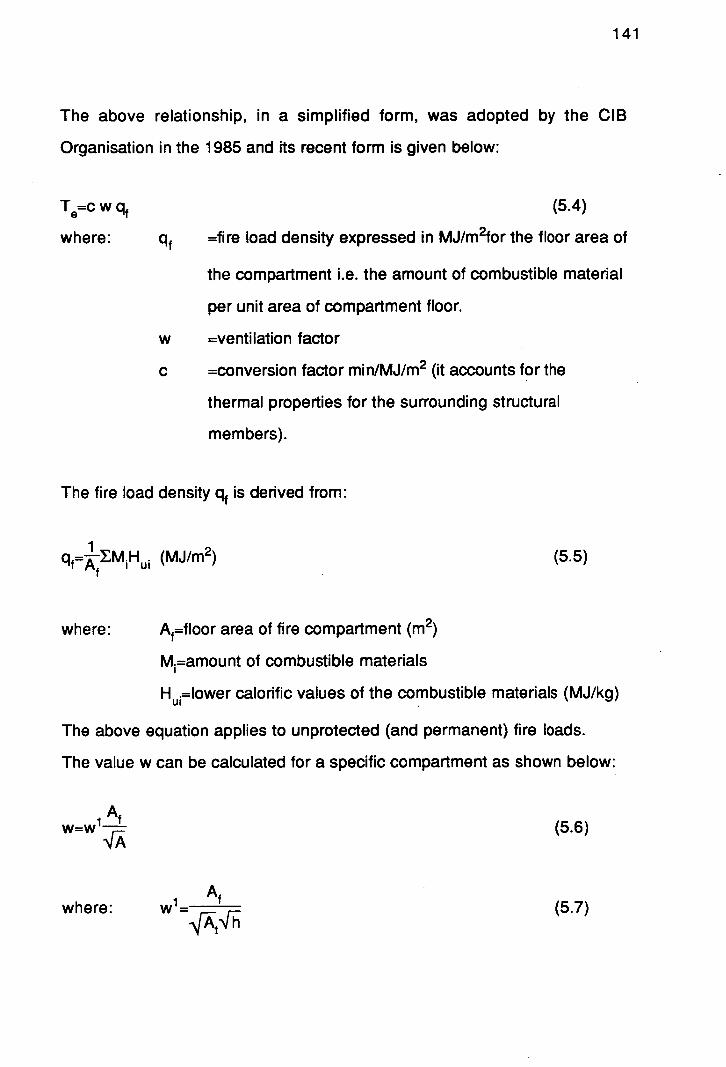
141

The above relationship, in a simplified form, was adopted by the CIB

Organisation in the 1985 and its recent form is given below:

T0=C w qf (5.4)

where: qf =fire load density expressed in MJ/m 2for the floor area of

the compartment i.e. the amount of combustible material

per unit area of compartment floor.

w =ventilation factor

c =conversion factor min/MJ/m 2 (it accounts for the

thermal properties for the surrounding structural

members).

The fire load density qf is derived from:

(MJ/m2 ) (5.5)

where: Af=floor area of fire compartment (m)

M 1=amou nt of combustible materials

H1=lower calorific values of the combustible materials (MJ/kg)

The above equation applies to unprotected (and permanent) fire loads.

The value w can be calculated for a specific compartment as shown below:

Af w=wt-

NFA (5.6)

A where: w1 = ._ (5.7)

142

A=floor area of the compartment (m 2 )

A=total area of floor and window openings (m 2 )

h=average height of the windows weighted

A=totaI interior surface area of the compartment

including openings.

The conversion factor c is related to the thermal properties of the enclosure

by means of thermal conductivity k and the heat capacity p cp which are

combined to render the thermal inertia b=Jkp cp.

Values of c to be adopted for various ranges of values of b are given in the

following table:

b( h' /2/M2 K) c (mins/MJ/m2)

Over 42 0.05

Between 12 and 42 0.07

Less than 12 1 0.09

Table 5.2 Conversion factor C

Values of the thermal inertia b for various materials are given below:

Normal weight concrete h 112/m2K)

Light weight concrete

t38

Aerated concrete 7

Steel 250 1 20 Brick

Timber 1 10

Table 5.3 Thermal inertia b

143

For medium weight construction, the value of c=0.07 can be adopted. The

value of c=0.1 will render a conservative estimate for different types of wall

lining.

A value of w=1.5 for the ventilation factor will provide a conservative

estimate corresponding to an opening area greater than 10% of the floor

area.

Equation (5.6) was basically derived for vertical opening areas. It is

recommended to confine the application of equation (5.6) to fairly high fire

compartments (H>>3.5m) and to average height of opening areas which are

well above ground level and are much larger than one metre (h>>1 .Om).

The greater effectiveness of horizontal roof openings may be considered by

calculating the total area A of the openings from the equation A=AV+afAh

with a1 equal or greater to one and Ah the horizontal opening area.

For office buildings, the average fire load density varies from less than 100

MJ/m2 in the lobby to 1500 MJ/m2 in file storage rooms. The Codes use 80%

fractile values i.e. 80% of rooms within the various occupancy groups have

fire load densities less than the value adopted in the calculation. For offices,

the 80% fractile values vary from 520 to 720 MJ/m 2 .

5.2. Codes related to the Performance of

Constructions in Fire.

5.2.1 BS 5950:Part 8 Code of Practice for Fire

Resistant Design

BS 5950:Part 8 [BSI, 1990] gives recommendations for the following

methods:

a' fire resistance derived from tests in accordance with BS 476: Part 20 -

21 [BSI, 1987].

b/ fire resistance derived from calculations.

144

The above methods may also be applied to members for which the required

fire resistance has been derived from the consideration of natural fires.

5.2.1.1 Fire Resistance derived from testing

Different test procedures are used for different types of construction. BS

476:Part 20-24 [BSI, 1987] presents the above methods within general

guidelines which are appropriate for the specific construction under test.

The common feature of all these methods is that the tested construction is

heated using the BS 476:Part 20 heating curve which is suitable for

simulating the thermal exposure encountered in a fire involving "cellulosic"

materials. To simulate hydrocarbon fires another temperature-time curve

must be applied i.e. MOBIL curve etc.

Failure is defined by a variety of criteria depending upon the function of the

component. For example, in the case of loadbearing members failure is

deemed to occur when they cannot support the test load.

The fire resistance of bare columns is taken either as the time to the limit of

stability or the limiting steel temperature of 550 °C for members loaded to

their maximum permissible design stress.

The fire resistance of columns in walls is normally taken as the time to the

limit of stability. Though the exposed portions of the members attain very

high temperatures, the applied load can still be supported by the much

cooler areas of the sections' profile which were protected by the blockward.

However, the steep temperature gradients created across the sections'

profile cause bowing. Of greater concern to the designer is the case where

the height of the wall is considerably greater than that evaluated in the fire

test.

Test data related to the fire behaviour of unprotected beams and columns

are presented in a British Steel publication "Compendium of UK Standard

Fire Test Data on Unprotected Structural Steel" [ASFPCM, 1988]. The series

145

of fire tests carried out on bare steel columns is limited. The columns are

standardized to a three (3) m length. The column ends are fixed. The column

is subject to nominally concentric axial load and the end moments are

negligible. Failure occurs when the rate of vertical or horizontal deflection is

so great that the load cannot be sustained.

The data applies to members which are loaded in fire conditions in

accordance with BS 449 ( permissible stress limits which are approximately

60% of the ambient temperature yield stress). Fire resistance can be unprotected

achieved for beams and columns of certain proportions. For columns in

simple construction (as defined in BS 5950: Part 1), according to fire test

results, a fire resistance of 30 minutes without fire protection is achieved if

the section factor H r/A does not exceed the value H/A=5O rn 1 "2 . In

practical terms, only very heavy steel members satisfy this limit. Lighter

sections can achieve 30 minutes of fire resistance if the applied load is

reduced.

5.2.1.2 Fire Resistance derived from calculation

The principal method of evaluating the fire resistance of structural members

is the "load ratio" method. According to this method, the temperature in a

critical part of the member (determined from the design temperatures or from

fire test data) is related to its reduced strength under fire conditions. The

load ratio gives a measure of the stress in the member at the fire limit state

relative to the design strength of the member. The higher the load ratio, the

higher the required retention of strength of the member in a fire, the lower

the temperature of the critical element to resist the applied loads. The

assumption under which the above method holds is that the members are

not subject to second order effect resulting from deflections during the fire.

146

5.2.1.2.1 Limiting temperature method

The fire behaviour of columns in compression, may be determined using

the limiting temperature method. According to this method, one can

determine the design temperature q at a required period of fire resistance

(Treq) the limiting temperature qL at factored load and compare them. Where

the limiting temperature is not less than the design temperature, the member

may be considered to have adequate fire resistance without protection.

When the limiting temperature is less than the design temperature,

protection must be provided.

Design temperature is defined as the temperature that the critical element,

the element of a section that would reach the highest temperature in fire

conditions, will attain at the end of the specified period of fire resistance in a

test in accordance with BS 476:Part 20 and 21 [BSI, 1987].

Limiting temperature is defined as the temperature of the critical element of a

member at failure under fire conditions and it depends on the following:

- the ratio of the load carried during the fire to the load capacity at 20 0C,

- the temperature gradient within the member,

- the stress profile through the cross section,

- the dimensions of the section.

The load ratio for columns exposed on up to four sides should be given by

the following according to the type of construction:

-For columns in simple construction, designed in accordance with BS 5950:

Part 1[BSI, 1985], the following equation holds:

Ff R=Ag Pc + + pyzy (5.8)

where: Ag=the gross area,

p=the compressive strength,

147

p, = design strength of the steel,

Z, = elastic modulus about the minor axis,

Mb = buckling resistance moment (lateral torsional),

F =axial load at the fire limit state,

MfX = maximum moment about the major axis at the

fire limit state,

MfY = maximum moment about the minor axis at the

fire limit state.

- For columns in continuous construction designed in accordance with BS

5950:Part 1, the following equations hold:

RF M1 M fY

=AgPy+M+Mcy or (5.9)

F M MfX MfY

R=AgPy + Mb + (5.10)

Mb are as defined above,

M,,as appropriate to the axis of bending, are the moment

capacity of section about the major and minor axes in the absence of

axial load,

m is the equivalent uniform moment factor.

Once the load ratio is determined, the limiting temperature for the applicable

load ratio is given in Table 5 [Appendix A] for different types of members.

The data in Table 5 [Appendix A] have been derived -where possible-from

tests. In some cases, they have been supplemented by computer modelling.

For compressive members of low slenderness (?.!5 70), the limiting

temperatures are based on test results supplemented with information from

the ECCS Recommendations. The test data on columns relates to

148

slenderness values less than 50 because of the restraints of the furnace. In

Table 5, the limiting temperatures have been extended up to a value

corresponding to a slenderness value less than 70 because this is the case

for columns in buildings.

It was found that the EGGS simplified column method provided an excellent

fit to the limited test data. The load ratio R is determined from the following

relationship:

A = Load multiplier x steel strength reduction factor

The load multiplier was taken as 0.85 (as in the ECCS Recommendations)

to take into account some end fixity of the columns and also the fact that on

average the steel should be stronger than the specified minimum. The

strength reduction factor is based on 0.5% strain in the steel because of the

relatively low strains that are experienced in columns just prior to failure.

For columns with slenderness ratio ?>70 and X:5180 , the adopted strain limit

is 0.5% and the load multiplier is increased to 1. The effect of end restraint is

less significant. High strains in the steel affect the stability of the member by

reducing the effective elastic modulus which leads to increased lateral

deflections. The use of an upper limiting temperature corresponding to a

load ratio of 0.3 avoids the potential risk of damage if normally stressed

members because of bracing, for example, are subject to additional loading.

For slender columns, the same as above apply. Slender columns benefit

more from continuity in a fire than stocky columns but because of lateral

restraint secondary forces and eccentricities may cause a reduction in the

column strength. The information related to the behaviour of slender

columns in a fire is very limited.

5.2.1.2.2 Design temperature

The thermal response of I section columns and beams has been measured

in the furnaces and correlated with analytical methods. For reference

149

purposes, these temperatures may be presented in terms of the section

factor (H r/A) or alternatively the flange thickness t f. For beams, the flange

thickness gives a slightly better measure of performance than the section

factor which is averaged over the cross-section. Columns exposed to fire

from four sides may be considered uniformly heated. In this case, the section

factor gives a good measure of the average temperature rise in the member.

The design temperature as defined in the previous Section depends on the

following:

-Section configuration

-Section dimensions

In the Code, design temperatures are presented as a function of flange

thickness for unprotected columns and beams.The data has been

determined partly from computer analyses using FIRES-T and partly from

fire tests. From BS 5950:Part 8 and for common periods of fire resistance,

the design temperature may be determined according to:

-Table 6 for unprotected columns and tension members,

-Table 7 for unprotected beams supporting concrete floors.

For periods of fire resistance other than those presented in the Code,

design temperatures can be determined from tests or by using computer

analysis.

5.2.2 European Recommendations for the Fire

Safety of Steel Structures.

The required performance of a structural element is defined in terms of a

particular failure criterion. This criterion may be either a limit of deformation

or the capacity to support a given load.

150

5.2.2.1 Deformation Behaviour -

Limit state of deformation

The analysis of the deformation behaviour is based on the material

properties of steel at elevated temperatures as given in the same document

where creep is taken into account implicitly. Using creep laws, the method of

calculation has been worked out so far only for beams.

The limit state of deformation is considered to be attained if it may be

assumed that actual failure occurs at extreme deformation, which has as a

result the function that adjacent members cannot be fulfilled and the spread

of fire to other rooms cannot be contained. The actual value of this limit of

deformation has an arbitrary character.

For beams and slabs in fire tests, the recommended deformation criterion

can be expressed as follows:

800h [mm] (5.11)

where: =max. deflection [mm]

=span [mm]

h=height of steel section [mm]

For a practical range of the span to height ratio, which is 15>j ->25, this

criterion tends towhere t represent the characteristic dimensions

described in Figure 5.1.

If the analysis is based on the determination of a complete deformation

behaviour, the deformation criterion can be checked. If the analysis is based

on the determination of the ultimate load bearing capacity, the deformation

will be unknown and the deformation criterion cannot be checked. However,

for practical values of the height to span ratio of structural steel members

and if no membrane forces are involved, the collapse criterion and the

deformation criterion, as described in the following Section, give similar

151

bv &hfj t 6IE[

(a) (b) (c)

characteristic dimension: (a)=t (b)=h

(c)= 6h (lateral deflection)

öi (vertical deflection)

Fig. 5.1 Characteristic dimensions (ECCS,1983).

152

values of fire resistance. There is therefore no need to check the

deformation criterion.

5.2.2.2 Ultimate Load Bearing Capacity -

Limit state of failure

The load bearing capacity at elevated temperatures can be calculated using

elementary plastic theory, where the same theory has been used at normal

temperatures (which implies that instability does not influence the load

bearing capacity significantly).

If the use of elementary plastic theory is prohibited, the reliability of the

method of calculation must be demonstrated explicitly. In the case of

columns, buckling curves at elevated tempeartures are recommended and

are derived from the EGGS buckling curves at room temperature. The

description of these curves is given in Section 5.2.2.3.

The limit state of failure is reached when the load-bearing capacity of the

structural load-bearing element or structural assembly decreases to the level

corresponding to the load considered to act on the structure under fire

conditions.The limit state of failure corresponds to an infinitely high rate of

deformation which is often almost impossible to determine because of

difficulties with the loading equipment or the limited depth of the furnace.

For beams, a maximum permissible deformation rate, which will be on the

safe side can be defined as below:

do dt ~ l5hx (5.12)

where: O=max deflection [mm]

[=span [mm]

h=height of the steel section[mm]

Mime

153

The combination of the deformation and failure criteria for beams , known as

the Robertson-Ryan criterion, is given below:

d8 12 dt ~ 15h [mm/h] and (5.13)

[mm/h] (5.1 4)

According to the Code, the above criteria does not apply to columns. In

contradiction to this statement, the same Code recommends the application

of the criterion of the maximum deflection not exceeding 1/30 th of the

characteristic dimension of the structural element under consideration for

columns as well as frames.

52.2.3 Buckling of steel columns

There is little information available for the solution of the stability problem

related to columns and their behaviour in fire environment. The reasons why

limited information exists are given below:

a' A very limited number of laboratories in Europe are equipped with

testing apparatus allowing full scale tests,

b/ The main effort has been placed on the evaluation of the fire

resistance of protected columns.

ECCS (European Convention of Constructional Steelwork) proposes a

design method, to tackle the stability problem in fire conditions, which is

based on the European Recommendations for Steel Construction at room

temperature.

154

- European Recommendations at room temperature

In the European Recommendations for Steel Construction, the ECCS has

proposed five basic buckling curves which are applicable to cross-sections

of different shapes.

The European curves are presented as relationships between N, the ratio of

the column critical stress to its yield stress,and its slenderness factor 1, the

ratio between the column slenderness ratio and the critical slenderness ratio

(5.15)

Because of the use of N and A., the curves are independent of the material

properties.

The analytical expression for the five non-dimensional buckling curves that

were adopted is as follows:

N = - A. 2 1 2 - 4? (5.16) 2A.2 2A.2

with

Curve a0 a b c d

a 0.125 0.206 0.339 0.489 0.756

Table 5.4

For beam-columns, where the moment or the load eccentricity has to be

taken into account, the same expression applies by introducing a factor r.

In this case, the following equations holds:

* 1+11 +A.2 1

s/[1 +1 * + A.2]2 - 4A. 2 (5.17) N= x 2A.2 - 2A.2

155

* e with = a (I - 0.2) + (5.18)

I Iv

where: eeq = equivalent eccentricity,

i= radius of gyration,

V= half the height of the profile.

- European Recommendations in fire conditions

In fire conditions, it is impossible to follow the same theoretical procedure as

the one developed by ECCS for bare steel columns at ambient temperatures

because the evaluation of the geometrical imperfections, the residual

stresses, the scatter of the yield stress within a cross-section, the stress-

strain relationship of the steel in compression and in traction e.t.c. is affected

by so many uncertainties.

The EGGS proposal for a design method adopts a range of buckling curves

corresponding to different temperatures which are derived from the EGGS

buckling curves at room temperature;

In order to transform the equations of the non-dimensional buckling curves

at room temperature to take into account the temperature variation,

variations of yield stress and Young's modulus with temperature have to be

included in the analytical equations for the fire situation. In the EGCS

Regulations, the equations describing the buckling curves at ambient

temperature are fitted to include the temperature effect by substituting are to

a,. and E. to E as follows:

N0 =k1 N and (5.19)

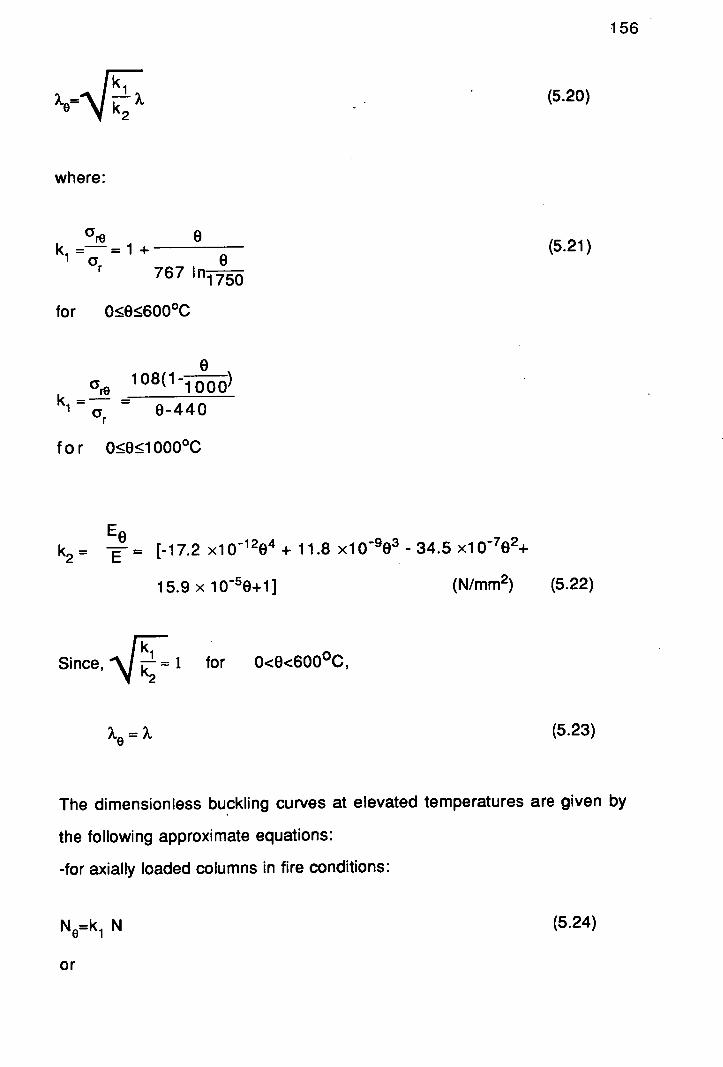
156

k ? e=

2 (5.20)

where:

CY r9 0 k ==1+ 1 e

767 In1750

for 050:5600°C

(5.21)

eare

108(1- 1

k1= = 0-440 Cyr

for 0:50!5i 000°C

E0 k2 = = [- 17.2 X10-1204 + 11.8 X10-9()3 - 34.5 xl 0 7e2+

15.9 x iOO+i] (N/mm2) (5.22)

Ic- Since, = 1 for 0<0<6000C,

= (5.23)

The dimensionless buckling curves at elevated temperatures are given by

the following approximate equations:

-for axially loaded columns in fire conditions:

N e ki N

(5.24)

or

157

° E1 -0.2) + ?2 -

— xsJ[ 1 + (?-O.2) + - CL 2] N =

0 Or 2? 2 2?.2

(5.25)

The coefficient a (dimensionless) varies with the selected curve and the

values are the same as at ambient tempearture.

-for eccentrically loaded columns in fire conditions:

* 0r9 1+ii+?.2 1

N0 = Or [ 2A.2 - —jx\J1 + TI +?] - 4)2

] (5.26)

The buckling curves in a fire environment that have been presented are

derived for bifurcation buckling. They do not take into account other types of

instability. For safety reasons, only curve "c is recommended at the present

time for all classes of profiles according to which the value of the coefficient

a is equal to 0.489.

The above design method has been compared with a large number of

experimental results obtained in Belgium, Denmark, and Germany on steel

columns in fire conditions with slenderness ratios varying between 25 and

167. The agreement is shown to be excellent and on the safe side after the

application of a correction procedure that has been introduced to achieve an

improved consistency between the analytical and experimental fire

resistances.

In the same proposal, since there is no criterion for buckling under fire

conditions in national or international standards, the time of failure is the

time at which the thermal elongation is cancelled out by the shrinkage of the

column. The advantage of this criterion is that it is easy to apply and

measure and that it is independent of the column length. This proposed

158

time of failure is not subject to interpretation and it is based on scientific

expenence.

5.2.2.4 Critical Temperature of Columns

The critical temperature of a load bearing steel element or structural

assembly is the temperature at which the limit state of failure is expected to

be attained.

The critical temperature of columns according to the result of a conventional

fire resistance test in which the test specimen is concentricily loaded may be

given by approximate rules based on the buckling curves (Section 5.2.2.3).

Under the above conditions of the standard test, the critical temperature can

be given from Figure 5.2 for a particular value of ratio of the effective yield

stress at elevated temperature to the nominal yield stress at room

tempearture (N,).

Assuming that the column failure occurs when the design load (kN*) equals

the critical buckling load (NCA a 20) the following equation holds:

kN=N cro A ay20 (5.27)

From the definition of coefficient iii, Ncre = it Ncr (5.28)

From equations (1) and (2),

kN = 41 NcrA a 20 = lf N. with Ncr=Ncr A 0y20 (5.29)

So, the limit state of failure is given by the equation:

1.0

0.8

0.6

0.4

0.2

159

0 200 400 600 800 1000


Fig. 5.2 Ratio ii of the effective yield stress at elevated temperature to

the nominal yield stress at room temperature as a function of

the steel temperature ( EGGS, 1983).

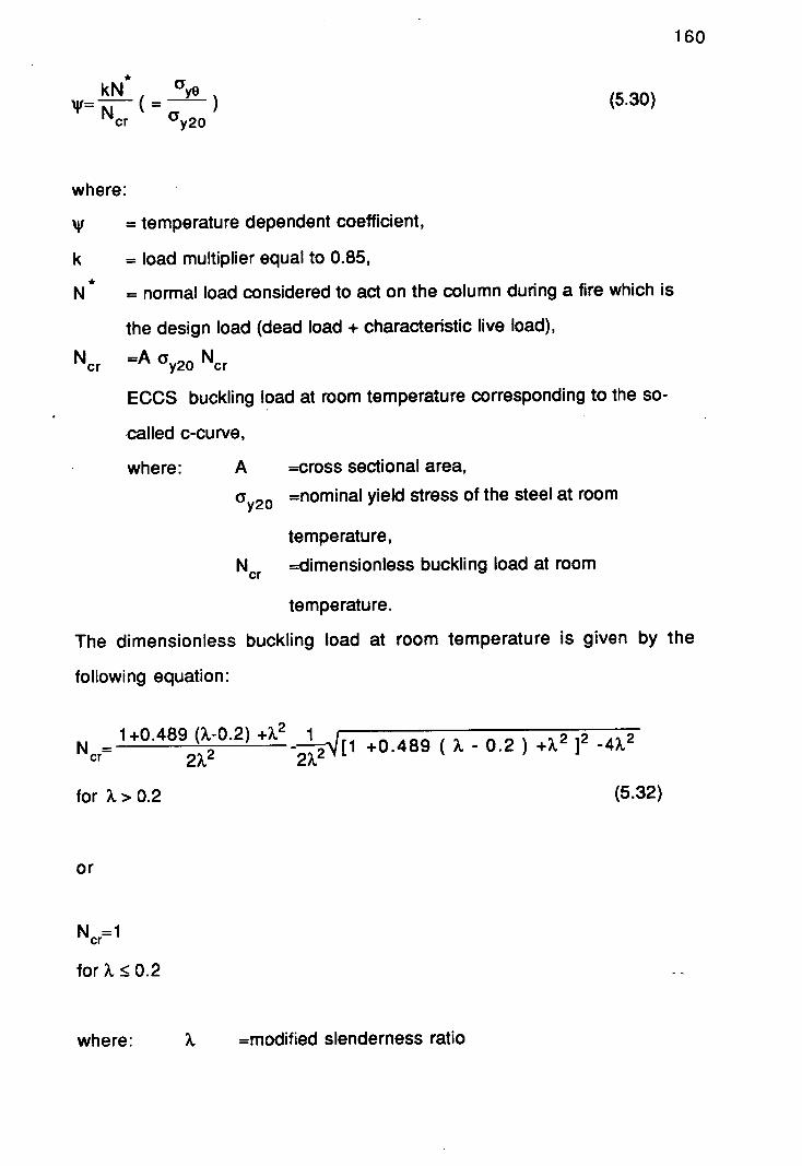
* kN a0

N cr aY2O (5.30)

160

where:

= temperature dependent coefficient,

k = load multiplier equal to 0.85,

N *

= normal load considered to act on the column during a fire which is

the design load (dead load + characteristic live load),

Ncr =A a,20 Ncr

EGGS buckling load at room temperature corresponding to the so-

called c-curve,

where: A =cross sectional area,

ay20 =nominal yield stress of the steel at room

temperature,

Ncr --dimensionless buckling load at room

temperature.

The dimensionless buckling load at room temperature is given by the

following equation:

1+0.489 (?-0.2) +X2 1 Ncr= 2?2

+0.489 ( - 0.2) j2 42

for A>0.2

or

Ncr=l

for 0.2

where: =modified slenderness ratio

(5.32)

161

lEq:E

(5.33)

=slenderness ratio at room temperature

E =modulus of elasticity at room temperature

=2.1 x 105 N/mm2.

In the above calculation of critical temperature, the normal load N is defined

as the design load (dead load + characteristic live load) which is considered

to act on the structure throughout the fire.

The above approach is rather conservative because the probability of the

occurence of a fully developed fire while, at the same time, the full

characteristic load is present is only very small. The possibility of reduction

of the live load should be introduced.

5.2.3 Fire Engineering Design Manual

If a steel temperature of 550°C is taken as the criterion for the onset of

failure, the 'fire resistance' of structural steel members can be calculated if

the temperature-time curve is known. The model developed by Pettersson et

al. (1976) can be used as input to iterative heat transfer calculations in order

to determine the 'fire resistance' of a particular member.

Pettersson has developed the above method further to analyse the stability

of the structural element (under load) at its maximum temperature taking into

account the temperature-dependence of the factors which determine the

strength of the steel, such as modulus of elasticity, yield stress e.t.c. In this

way, a definition of a 'failure temperature' has been avoided.

In Figure 1 [Appendix C], a flow chart which illustrates the design procedure

according to Pettersson is given. Following this procedure, one must

determine the static load which shall not cause the structure to collapse

162

under fire exposure conditions,the design fire load and the opening factor.

Conversion of the fire load and opening factor for the fire compartment in

question into equivalent fire load and opening factor follows. If the fire load is

low and the conditions are favourable in other respects, one has to check if

the structure can be constructed without insulation or wherever it has to be

protected. For unprotected structures, one has to determine the resultant

emissivity, calculate the F IV ratio and determine the maximum steel

temperature. For columns, the degree of expansion has to be assessed if

expansion is restrained, and the critical load has to be determined. To

determine the critical load, the designer has three cases to design for:

-compression only,

-Simultaneous flexure and compression,

-the risk of out-of-plane instability.

Design Static Load

Pettersson, regarding the determination of design static load, divides the

buildings according to their design and type of activity as follows:

-buildings in which complete evacuation of people in the event of fire cannot

be assumed,

-buildings in which complete evacuation of people in the event of fire can be

assumed.

Buildings in which complete evacuation of people in the event of

fire cannot be assumed

In buildings such as large hotels, blocks of flats and offices, it is not possible

to assume that complete evacuation of people takes place in the case of a

fire. In this way, the design has to include the possibility of fire being in

progress in limited parts of the building without complete evacuation of

people taking place. In this type of building, the designer has to show that

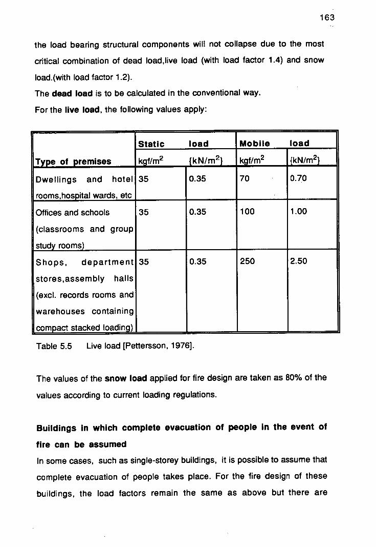
163

the load bearing structural components will not collapse due to the most

critical combination of dead load,Iive load (with load factor 1.4) and snow

Ioad.(with load factor 1.2).

The dead load is to be calculated in the conventional way.

For the live load, the following values apply:

Static load Mobile load

kgflm2 {kN/m 2 } kgflm2 {kN/m2 } Type of premises

Dwellings and hotel 35 0.35 70 0.70

rooms,hospital wards, etc

Offices and schools 35 0.35 100 1.00

(classrooms and group

study rooms)

Shops, department 35 0.35 250 2.50

stores,assembly halls

(excl. records rooms and

warehouses containing

compact stacked loading)

Table 5.5 Live load [Pettersson, 1976].

The values of the snow load applied for fire design are taken as 80% of the

values according to current loading regulations.

Buildings in which complete evacuation of people in the event of

fire can be assumed

In some cases, such as single-storey buildings, it is possible to assume that

complete evacuation of people takes place. For the fire design of these

buildings, the load factors remain the same as above but there are

164

differences regarding the values of live load (mobil load particularly) which

are given below:

Static load Mobile load

kgf/m2 {kN/m2} kgf/m2 {kN/m2 1 Type of premises

Dwelling and hotel 35 0.35 35 0.35

rooms,hospital wards, etc

Offices and schools 35 0.35 55 0.55

(classrooms and group

study rooms)

Shops, department 35 0.35 70 0.70

stores,assembly halls

(excl. records rooms and

warehouses containing

compact stacked loading)

Table 5.6 Live load [Pettersson, 1976].

The values of the mobile load are changed because of the evacuation of the

building in the event of fire.

In some cases, the designer has to estimate the local increase of the live

(mobile) load which may increase due to people moving from the part of the

building which is affected by the fire to another part of the building or in

conjuction with the evacuation of the building.

The above values, concerning loads and load factors, are conservative.

165

Design Fire Load

The fire load in a fire compartment is the total quantity of heat released upon

complete combustion of all the combustible material contained inside the fire

compartment, inclusive of building frame, furnishings, cladding and floor

coverings.

The fire load per unit area is given by the total internal surface area of the

fire compartment and is calculated from the relationship:

q= At (Mcal/m2) {MJ/m2}

(5.34)

where:

m= the total weight of each individual combustible

material constituent, v, in the fire compartment

(kg),

H= the effective calorific value of each individual

combustible material constituent, v, in the fire

compartment (Mcavkg) {MJ/kg},

At the total internal surface area of the fire compartment

(walls, floor and ceiling) (m 2).

Complete combustion of all the combustible material in a fire compartment

does not take place during a fire.

The fire load per unit area can be calculated, to take into account the degree

of combustion of each fire load component, by the following relationship:

Ep.mH q= At (5.35)

.

166

where: vv= a non dimensional factor with a value between 0 and 1

which indicates the actual degree of combustion for

each fire load component ,v.

For example, bookcases and floor coverings that have a

very low degree of combustion, have .t values

appreciably below unity.

The effective calorific value of some solid, liquid and gaseous materials are

given in the following Table:

Solid Effective Liquids Effective Gases Effective

Materials Calorific Calorific Calorif Ic

value(H) value(H) value(H)

Dry Mcal/kg Mcal/kg Mcal/m3n

materials x4.2{ MJ/kg} x4.2{MJ/kg}

Clothes 4.0-5.0 Crude oil 10.3 Acetylene 13.6

Leather 4.0-5.0 Diesel 9.7-10.1 Carbon 3.0

oil Monoxide

Polyvinyl 4.4-5.2 Paraffin 9.8 Coal gas 4.0

Chloride(PVC)

Rubber waste 5.0 Petrol 10.4 Hydrogen 34.0

Paper and 3.8-4.2 Spirits 7.6-8.2

cardboard

Wood 4.1-4.7 1 Tar 9.0

Moist

I materials

HF=H( 1 -0.01 F)-0.006F

167

Iwhere: F=moisture content

lof material in % by weight

Table 5.7 Effective Calorific Values

[Pettersson (1976)].

According to the above, the design fire load can be determined by direct

calculation {Equation (5.34) and (5.35)}. However, the designer requires

sufficient knowledge of types and quantities of furniture and fittings in the

building. Equation (5.35) is more difficult to apply due to a lack of

experimentally substantiated and verified values of g.

To allow for any future alterations or rearrangements in the building, the

design must not be rigid regarding these aspects. It is safer therefore to base

the design on statistical investigations concerning the magnitude of the fire

load for the type of building in question (Table 2, Appendix C).

The above interpretation of the fire load is valid for a uniformly distributed fire

load inside the fire compartment. This assumption does not introduce

problems caused by the violent turbulence which develops during the fire

causing small temperature differences in different parts of the compartment.

The present design method does not cover the case where the fire load is

extremely uneven and causes significant temperature effects in certain

structural elements.

Opening factor

Pettersson presents a procedure whereby it is possible to calculate the

temperature-time curve of the fire process (both the flame phase and the

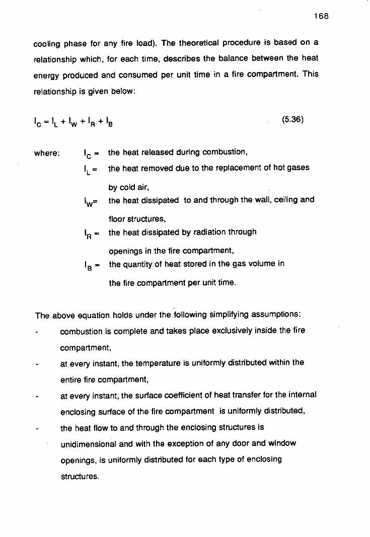
168

cooling phase for any fire load). The theoretical procedure is based on a

relationship which, for each time, describes the balance between the heat

energy produced and consumed per unit time in a fire compartment. This

relationship is given below:

'C = 'L + w + ' R + 'B (5.36)

where: IC = the heat released during combustion,

= the heat removed due to the replacement of hot gases

by cold air,

lw the heat dissipated to and through the wall, ceiling and

floor structures,

In = the heat dissipated by radiation through

openings in the fire compartment,

'B = the quantity of heat stored in the gas volume in

the fire compartment per unit time.

The above equation holds under the following simplifying assumptions:

- combustion is complete and takes place exclusively inside the fire

compartment,

- at every instant, the temperature is uniformly distributed within the

entire fire compartment,

- at every instant, the surface coefficient of heat transfer for the internal

enclosing surface of the fire compartment is uniformly distributed,

- the heat flow to and through the enclosing structures is

unidimensional and with the exception of any door and window

openings, is uniformly distributed for each type of enclosing

structures.

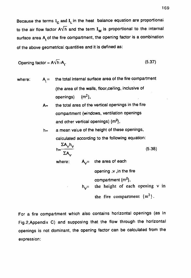
169

Because the terms 1 and IL in the heat balance equation are proportional

to the air flow factor AFh and the term 1 is proportional to the internal

surface area At of the fire compartment, the opening factor is a combination

of the above geometrical quantities and it is defined as:

Opening factor = A/A. (5.37)

where: At the total internal surface area of the fire compartment

(the area of the walls, floor,ceiling, inclusive of

openings) {m2 },

A= the total area of the vertical openings in the fire

compartment (windows, ventilation openings

and other vertical openings) {m 2},

h= a mean value of the height of these openings,

calculated according to the following equation:

YAvhv h= (5.38)

IAv

where: A= the area of each

opening ,v in the fire

compartment {m 2},

h= the height of each opening v in

the fire compartment (m 2 ).

For a fire compartment which also contains horizontal openings (as in

Fig.2,Appendix C) and supposing that the flow through the horizontal

openings is not dominant, the opening factor can be calculated from the

expression:

170

where: (A I

A, ) =the opening factor for the vertical

openings (m 112 )

f k =correction coefficient from the

nomogram in Fig.5.3_given as input

data the ratios (A\j h 1 /AJh) and (A-5-/A)

and the fire temperature in the compartment

in question.

When the flow of air and gases takes place mainly through the horizontal

openings, the flow becomes unstable and difficult to describe by means of a

simple theoretical model.

The above calculation for opening factor assumes that the windows and

doors are immediately destroyed when a fire breaks out. This assumption is

valid for doors and windows with ordinary glass but it does not directly apply

to doors of a certain fire resistance or windows with reinforced glass. In the

latter cases, to be on the safe side, the design has to be carried out using a

value of opening factor whereby the calculation will give a higher maximum

temperature of the steel structure.

Conversion to equivalent fire load and opening factor

Using the design data presented in the form of tables and diagrams in the

Swedish Fire Engineering Design Manual [Pettersson, 1976], the designer

can directly determine the maximum steel temperature, with the restriction

that the compartment in question must be identical with the description of the

fire compartment type A (characterised by its surrounding construction and

given in Table 3, Appendix C).

Area: /

' A b'h1 ••'' . -

V1

Fig. 5.3 Nomogram for calculation of the coefficient

(Pettersson, 1976).

171

172

The above mentioned design data may be used for the design of other types

of fire compartments by converting the temperature-time curve in the

compartment in question into the temperature-time curve in the fire

compartment type A. Employing a factor Ic 1 , the actual fire load and opening

factor can be converted into an equivalent fire load and opening factor by

multiplying the actual values by kf .

Values of k1 are given in Table 3 (Appendix C) for different types of fire

compartment (characterised by their surrounding construction) and as a

function of the size of the opening factor. In some cases, the value of k1 can

vary as a function of the magnitude of the fire load as well.. Because the

relationships used to determine the factor k 1 are not linear, its values

determined by linear interpolation for types of compartment differ from those

listed in Table 3 (Appendix C). The fire compartments used in interpolation

therefore should be those which yield the lowest values of k1 . In determining

kf , a combination of different types of fire compartments cannot be made

which results in a negative contribution for k1 .

The temperature-time curves for fire compartment type A for variable fire

loads (q) and opening factors (A'[i/A), given in Figure 5.3, are based on the

assumption that the combustion process is ventilation controlled and the

mean rate of the combustion of wood (in kg per unit time) during the flame

phase is known and proportional to the air flow factor (A\[i).

The fire load controlled combustion process is complicated due to

uncertainties involved regarding the determination of the rate of combustion,

the size of the fire load, the method of storage and the degree of distribution

of the fuel. Except for fire compartments with large openings, in which fire

load combustion process mainly occurs, there is no reliable theoretical

model available to assess the flow configuration. The gas flow through

openings, with velocity components in both the horizontal and vertical

directions, reduces the interchange of gases between the fire compartment

173

and its surroundings. For gas flow through the small openings, it has been

confirmed experimentally that the horizontal velocity component is the

dominant one. So, because of the uncertainties listed above, it is rather risky

for the designer to assume a fuel-controlled fire

A CIB research programme which examined fully developed fires, showed

that a maximum well was within the ventilation-controlled regime (Fig 5.4).

Assuming a fuel-controlled fire is less severe, savings can be made on the

cost of structural fire protection. Because of the complexity of the problem

and the uncertainties involved (as stated above), it is recommended that the

design should assume a ventilation-controlled fire. This yields results on the

safe side.

Resultant emissivity Cr

Radiation is the trasmission of energy by electromagnetic uwaves ! .

A surface which absorbs all radiation incident upon it is called a black

surface (e=1).

Real surfaces are less efficient absorbers and emitters than black surfaces

(e<1) and their absorptivity and emissivity depend on the wavelength, X.

Emissivity is then defined as follows:

E(?.)

c( - Eb() (5.40)

where: E(k) =the emissive power at wavelength I

Eb(A) =total emissive power of a blackbody

at wavelength ?

=cyT4 {kW/m2} with (Y=56.7x1 012 {kW/m2K4}

(Stefan- Boltz man Constant) (5.41)

i Limit of ventilation control 1000 00_

vc

5O00C I

FC increasing ventilation

0 10 20

30 40

A1./AH 112

Fig. 5.4 Fuel - controlled and ventilation - controlled fire

regimes (Drysdale, 1989-90).

174

175

Grey surfaces are the ones for which emissivity .is independent of

wavelength. Emissivity is then defined as follows:

E (5.42)

where: E =the emissive power of a grey body

=eaT4 {kW/m2} with a=56.7x1 0-12 {kW/m2}

(Stefan-Boltzman Constant)

The resultant emissivity (Cr) 5 dependent on the emissivities of the flames

(et) and the steel structure (es), on the sizes of the flames and the steel

structure and their positions relative to each other.

For the simple case of two infinitely large parallel surfaces where all

radiation from the one surface falls on the other surface and vice versa, the

resultant emissivity is given below:

1

Cr=l 1 —+--1

E Cs

(5.43)

where: Ct = emissivity of the flames

=1- c1 Xf with Xf flame thickness (m) (5.44)

=1 for thick flames

<1 for thin flames

= emissivity of the steel section

(treated as a grey body)

176

For a column exposed to fire on all sides, the emissivities of the flames and

the steel structure are assumed to be 0.85 and 0.80 respectively which give

a resultant emissivity of Cr=0•7 For the case of a column outside a facade,

because it is exposed to less radiation, a value of can be used.

Recommended values for use for resultant emissivity er,which yield results

on the safe side, are given in Table 5a.

F 8/V8 ratio

where FS is the fire exposed surface of the steel section and

V is steel section volume per unit length

The FS/VS ratio varies as a function of the section dimensions and the

method of construction.

Values of the ratio FS/VS are given in Table 5b for rolled I-profile sections

exposed to radiation on all sides and with one flange concealed. Examples

of calculation of the ratio FS/VS for different types of construction are given in

Figure 3 (Appendix C).

Maximum steel temperature

The quantity of heat transferred to the steel section per unit length and over

a short interval is as follows:

Q = a F(O - O) At (kcal/m) {J/m} (5.45)

where: a = the surface coefficient of heat transfer of the

boundary layer

5.77cr 0 t 4 S +273 0 +273

+ ( 4

=23 0 - 0 s [( 100 - 100 ]{W/m2°C}

(5.46)

FS =the surface of the steel section per unit length

exposed to fire (m2/m),

Ot =the gas temperature in the fire compartment at

time t (°C),

O S =the temperature of a steel section at time t ( °C),

At =the length of time interval (h) {s}.

This quantity of heat per unit length causes the temperature of the steel

section to rise by an amount determined by the thermal capacity of the steel

as given below:

Q =Cps AO Vs ys (kcal/m) {J/m} (5.47)

where: Cps= the specific heat capacity of the steel

(kcal/kg °C) {J/kg°C},

AO S =temperature rise in the steel section ( °C),

V =volume per unit length of the steel section

(m3/m),

ys =density of the steel (kg/M 3 )

=7850 kg/m3

By equating (a) and (b):

a FS AO= -

YS Cps V S (° - O) At (°C) (5.48)

In order to derive the increase of the steel temperature over a short time

interval, the following assumptions have been made:

177

178

-the heat flow is unidimensional,

-the steel section is heated uniformly at any time.

The first assumption can be satisfied assuming that the structural element in

question is of infinite length and the corners are so small they do not affect

the validity of the calculation.

The second assumption is satisfied when the actual structural element is not

subjected to thermal gradients of significant value (column built into a wall

with one flange and part of the web exposed).

The maximum steel temperature derived from equation (5.48) is dependent

on the F5/V 5 ratio, the value of the resultant emissivity Er , the gas

temperature O in the fire compartment which is determined on the basis of

the opening factor and the fire load of the fire compartment.

Maximum temperature values calculated by computer using equation (5.48)

for the fire compartment type A are presented in Table 6 (Appendix C].

Critical load

Steel structure subject to an axial compressive force.

At ambient temperatures, one may design steel columns subjected to axial

loading and against buckling employing two principal methods which apply

to the design of:

- initially straight columns,

- columns of representative initial curvature and unintentional load

eccentricity.

According to the first approach which deals with the design of initially

straight colunms, the stress-strain curve of the material in question is taken

into account and the ideal buckling load is more often determined by the

tangent modulus theory. The permissible buckling load is obtained by

dividing the buckling load by a safety factor to take into account the initial

179

curvature and unintentional load eccentricity. The safety factor is dependent

on the slenderness ratio of the column.

According to the second approach which deals with the design of columns of

representative initial curvature and unintentional load eccentricity, the

maximum compressive stress in the column is determined. The critical axial

compressive force is defined as the compressive force which causes the

maximum compressive stress to attain a value which is either the yield

stress or the 0.2% proof stress of the material. The permissible compressive

force is obtained by dividing the buckling load by a safety factor which is

independent of the slenderness of the column.

For the latter group and for a column which is free to expand while heated,

the buckling stress (a k) can be calculated by the following expression:

kk =-a02 2 (5.49)

where: ak =buckling stress (kgf/cm2) {MPa},

a02 =yield stress or 0.2% proof stress at the actual

steel temperature (kgf/cm2) {MPa},

E =modulus of elasticity at the actual steel

temperature (kgf/cm2) {MPa},

LL =T =effective slenderness ratio,

where: L =length of the column (cm) {m},

=nondimensional coefficient,

=the radius of gyration of the cross-

section with respect to the neutral

axis through the centroid (cm) {m}.

In the above equation (5.49), the initial curvature and the unintentional

eccentricity have been taken into account in the calculation. They were

180

included in the form of a pure initial curvature, the maximum value of which

is given below:

f=4.8x105 (f3L)2

d (5.50)

where: d =distance of the neutral axis to the extreme fibre of the

cross section in compression at the section which

governs design (m).

The nondimensional coefficient pis a function of the fixity conditions of the

column, the variation of cross section and the variation of the axial

compressive force along the column.

The stress a02 can be determined from the stress-strain curves of the steel

material in question at different steel temperatures. Because the stress-strain

curve at elevated temperatures is softly rounded, to obtain a better

approximation of the buckling stress, the secant modulus of elasticity is used

instead of the initial modulus of elasticity and the 0.2% proof stress (a 02 )

instead of the 0.5% proof stress (a 05).

Applying the above relationship ( 5.49 ), calculated relationships between

the buckling stress and the slenderness ratio for steel columns made of

materials with yield stresses at room temperature of 220,260,320 {MPa} at

different temperatures 9 have been obtained. These are presented in

Fig.5.5. The temperature - dependence of the proof stress 0.5% and the

stress and temperature dependence of the secant modulus E (as in Fig. 5.6)

are taken into account for the calculation of the ?. curves. These material

properties have been determined from tensile tests where the test

181

Fig. 5.5

Calculated relationships between the

buckling stress crk and slenderness

ratio I for steel columns made of

materials with yield stresses at room

temperature of as = 2200 {220},2600

{260}, 3200kgf/cm 2 {320MPa} at different

temperatures O. The diagrams apply to

columns which are free to expand

longitudinally ( Pettersson, 1976 ).

0,

- -. -

I

a 2200 kgf/cm 2 220

- -\ lMPaj

-- -- .........

700

N 450 -

/ PQ I5Q

= = 1 U b() 100 15()

c1

200 - 30M A -

-

too

SOC f5c

-

260 '\ \ _260 JMP21

-- .. .\ \

-

0kgf/cm 2

\\\ 'i(b - -. 20()

- - 3(X) -- ........ ............

-- - .\\71PO

- -- - -- - -

/ 450 --.--..''..-' '\'- f . :••

55Q GO0

.-'-z.

.III. -

100 150 200 X

0- - • 320 IMPaI

25(X)-— \._.. - ...- ...................- 12501 "

- \

2O0O — -\ 12001 - . . -

N

\ \\N'oc \l\ 100

'

11501 0 300

• \ \ ' [350

10(X)- • \\

Y.Ir9 (100) .

N \ /150

60(

Isol

A

E,cy05

0/ /0

10C

8C

60

40

20

200 400 600°C

182

Fig. 5.6 The modulus of elasticity (secant modulus) E as a function of

the steel temperature O for different values of the ratio of the

stress a to the yield stress at room temperature 0• The dashed

curve indicates the variation with temperature of the 0.5% proof

stress ( Pettersson, 1976)

183

specimens were loaded at a constant rate of loading of 18 kgf/cm 2/min (1.8

MPa/min) ito include the effects of the short- term creep.

In this way, from the above mentioned Gk-A curves, for a max steel

temperature °max (Table 6 for uninsulated columns) and a slenderness ratio

A, the critical stress can be obtained and the buckling load of the column is

calculated as follows:

Nk k= (kgf/cm 2) {MN/m2} (5.51)

where: N=buckling load of the column (kgf) (MN),

A=area of cross section of the column (cm2){m2}.

The design criterion for the loadbearing function is that the minimum

loadbearing capacity given by the buckling load (Nk) must not be less than

the axial force the cross section is subjected to.

When the longitudinal expansion of the column is partially prevented in a

fire, the compressive force in the column increases and the column buckles

at a lower imposed external load. The longitudinal expansion can be

partially prevented because of the reduced value of the modulus of elasticity

of steel as the steel temperature increases or because of the adjacent

structural elements.

The reduction in the expansion of the column due to reduced value of the

modulus of elasticity is:

NL11 1 (cm) {m}

(5.52)

where: E =modulus of elasticity (secant modulus) of the steel at

the stress and steel temperature in question

(kgf/cm2) {MPa},

184

E0 =modulus of elasticity of the steel at ordinary room.

temperatures (kg f/cm 2) {MPa},

A =area of cross section of the column (cm2) {m2},

N =magnitude of the compressive force (kgf) {MN}.

The expansion of an unloaded steel column when there is no restraint on

longitudinal expansion is:

AL'=aO 5L (cm) {m} (5.53)

where: a =coefficient of linear expansion ( °C 1 )

es =steel temperature ( °C),

L =original length of the column (cm) {m}.

So, the resultant expansion AL of the column is:

1 AL=AL'-AL=aO5L- NL 1 - A -(- --) (cm) (m) (5.54)

The reduction in the expansion of the column because of the adjacent

structural members is:

ALr = 'y AL (cm) {m}

(5.55)

where: 7 =degree of expansion, a nondimensional

coefficient with values between 0 and 1.

=1 (no restraint on longitudinal expansion)

=0 (the expansion is completely prevented)

185

Determination of the degree of expansion y according to the above equation

is a complicated process. Values of the degree of expansion 'y for some

common cases are given in the diagram in Figure 4 (Appendix C).

Critical buckling stresses as a function of the steel temperature, slenderness

ratio and degrees of expansion for steel columns made from materials with

yield stresses of 220, 260, 320 MPa at ordinary room temperatures are given

in Figure 5 (Appendix C). Apart from the degree of expansion, there is

another parameter , the cross sectional factor i/d, the effect of which is

relatively limited. For the curves in Figure 5 (Appendix C), the value i/d=0.5

was used for the calculation which for the normal type of cross section yields

results on the safe side.

The above described design approach for the calculation of the buckling

load is in good agreement with full scale tests. More accurate design based

on the actual stress-strain curves would produce the deflection curve of the

steel column and the a k - ?. curves will be dependent (apart from the

maximum steel temperature) on the rates of heating and cooling as well.

In plane instability checks have to be carried out in the following cases:

- when the column subject to an axial compressive force is braced by

adjacent structural elements against deflection at right angles to the plane of

bending.

- when deformation can freely occur out of the plane of bending and

the line of action of the axial compressive force coincides with the shear

centre of the cross section.

In all the other cases, a slender column subjected to an axial loading must

be checked for out-of-plane instability.

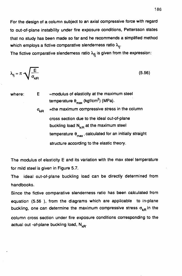
186

For the design of a column subject to an axial compressive force with regard

to out-of-plane instability under fire exposure conditions, Pettersson states

that no study has been made so far and he recommends a simplified method

which employs a fictive comparative slenderness ratio A.f .

The fictive comparative slenderness ratio A.t is given from the expression:

Xfj (YE (5.56)

JdR

where: E =modulus of elasticity at the maximum steel

temperature Om (kgf/cm2) { MPa}.

aR =the maximum compressive stress in the column

cross section due to the ideal out-of-plane

buckling load NkjR at the maximum steel

temperature 0max calculated for an initially straight

structure according to the elastic theory.

The modulus of elasticity E and its variation with the max steel temperature

for mild steel is given in Figure 5.7.

The ideal out-of-plane buckling load can be directly determined from

handbooks.

Since the fictive comparative slenderness ratio has been calculated from

equation (5.56 ), from the diagrams which are applicable to in-plane

buckling, one can determine the maximum compressive stress okAin the

column cross section under fire exposure conditions corresponding to the

actual out -of-plane buckling load, NkR.

Ete

in

N/mm2 2.0

1.5

1.0

0.5

xi 05

0 200 400 600 1 800 1000


Fig. 5.7 Modulus of elasticity Et. as function of the steel

temperature (ECCS, 1983).

187

IM

5.2.4 Discussion

Fire resistance periods

The background to the objectives of the Building Regulations concerned

with the behaviour of structural elements in fire, as well as the time

equivalent calculation methods which define fire resistance requirements for

elements of structure, has been reviewed. Though the fire engineering

approach is sound, one has to be concerned with the accuracy and the

limitations of the fire severity equations as well as the assumptions made for

the determination of the fire load density.

In actual practice many more factors affect fire severity than those taken into

account so far. Fire severity is affected by the fire load, surface area, fire load

arrangement, wind and the properties of the walls of the fire compartment.

The influence of all these factors is substantial. They may cause deviations

of the order of 50% from the predicted fire severity. In comparison with the

influence of the two most important factors, fire load and opening factor,

which can have values in practice in a range extending over a factor of 10

their influence is relatively small. Therefore, it is justifiable to express the

correlation between critical fire load and fire severity only in terms of the

most important factors, and to take into account the influence of the other

factors, which are often unpredictable and uncontrollable, by incorporating

an appropriate factor of safety in the fire resistance requirements.

Because relatively small scale tests have been conducted to establish the

fire severity relationships, also the fire load involved was timber, the above

equations may not hold for the case of large compartments.

The determination of the value of the fire load and the fire load density is

critical when using the fire severity equations. Usually, the values of the fire

load are derived from several surveys of fire loads and are given in various

design Codes. The problem is that the surveys have been carried out some

189

time ago and the character of various occupancy groups may have changed

since the original surveys.

For large inter - connecting spaces in multi - functional buildings, it is difficult

to determine the size of the openings.

If the function of the compartment is changed and the elements are designed

with small factors of safety, upgrading may be necessary.

Standard tire resistance tests [Witteeveen, 1981/82]

In the conventional BS 476 : Part 20 - 24 [BSI, 1987] fire tests, failure is

defined as the time when the member can no longer support the test load

which means that the load bearing capacity of the construction is reduced

below the applied load. The fire environment is the one as defined in BS

476 and stability has been generally measured on fully exposed single

elements subject to the maximum permissible load to simulate the worst

possible case.

Data derived from conventional fire tests can be used to define failure

temperatures which will depend on steel quality, degree of loading and

structural features like composite action, restraint and continuity. The steel

failure temperature of 550 °C is usually adopted for the assessment of results

from single element fully loaded fire tests where the temperature distribution

throughout the members' cross section is uniform.

Though the fire resistance tests have been performed for more than a

century without major changes in test procedure, some serious weaknesses

can be observed. Factors like the the heat-flow characteristics of furnaces,

variation in material properties, geometrical imperfections, residual stresses,

temperature distribution across and along the members and restraint

conditions may cause significant differences in test results of structural

elements under the same load repeated in the same furnace (repeatability)

or tested in different furnaces (reproducibility).

190

For columns, the length of the specimen generally varies between 3 and 4 m

and in view of the capability of most of the existing furnaces the loading must

be applied centrically and is kept constant during the test which is a rough

approximation of the real situation where the column is loaded by both

normal forces and bending moments. Because the design load

specifications may be different from country to country, the test report must

give detailed information about this matter in order to have comparative

results when the test is reproduced in a different furnace. Another factor that

affects repeatability as well as reproducibility of the test results is that neither

the test load nor the test results are adjusted to take into account the

difference between the actual random values and the characteristic values

of the material strength, imperfections and residual stresses.

The determination of the ratio between the test load (P) and the ultimate

load-bearing capacity (P 1 ,20) at room temperature is of more importance than

the actual test load. The ultimate load bearing capacity (b2o) is a function of

the yield strength for relatively small slenderness ratios (0.12) and a function

of the modulus of elasticity for relatively high slenderness ratios (0.04). The

coefficient of variation of the yield strength, which is well known from

extensive investigations, is higher than the coefficient of variation of the

modulus of elasticity. The load bearing capacity is also influenced by initial

geometrical imperfections and residual stresses, the coefficient of variation

of which is difficult to quantify. The yield strength of a random sample is

higher than the characteristic value on which the design load is based. The

level of imperfections and residual stresses is lower than the characteristic

values specified in the Regulations and Codes. In this way, the ratio 'b20

of a random test specimen will be lower than the design value which varies

according to national specifications between 0.6 and 0.7. In a standard fire

test, assuming a coefficient of variation of load bearing capacity equal to

0.08, the ratio P/Pb20 will have a value between 0.5 and 0.67 for most cases.

191

The heating characteristics of the furnace, as well, as the manner of

exposure, influence the temperature variation in the longitudinal direction of

the column which will affect the reproducibility of the test results. For pin-

ended columns, the effects of a non-uniform temperature distribution on the

critical temperature is smaller than for columns with both ends built in.

Critical temperature is defined as the temperature at collapse at mid-height

of the column.

In a fire resistance test, the test specimen shall be supported and restrained

in a manner which is as far as possible similar in nature to the

corresponding structural element in service. In a real building, a column has

rotational restraints which depend on the stiffness of the surrounding

structural elements. In a column furnace, the loading device provides fixed

rotational restraint, either pin-ended or one end fully built in and the other

end pin-ended. In most of the cases, the real degree of restraint is quite often

unknown and may vary during the test. Axial restraint is not accounted for in

standard fire resistance tests. For tests on pin-ended columns, even a small

degree of unintended rotational restrained, which is unavoidable, has a

significant influence on the critical temperature. Fully built-in columns are

less sensitive to small changes in restraint. Though fully built in columns are

more sensitive to a non-uniform temperature distribution, the influence of

the degree of restraint of pin-ended columns on the critical temperature is

more critical. So, fire resistance tests on columns fully built in at both ends

give more reliable results than the pin-ended ones.

Unavoidable eccentricity of the load results in a combined action of normal

force and moment and may cause problems of repeatability as well as

problems of reproducibility. It is better to prescribe a certain eccentricity of

the load and to account for this eccentricity when determining the load level

to be applied.

192

The factors responsible for inadequate reproducibility are dependent on the

heating characteristics and the mechanical characteristics of the loading

device of the furnace in question. In order to have better results, the above

characteristics must be standardized.

As a conclusion, the fire resistance tests provide a poor instrument for the

classification of fire exposed steel columns especially if the design is based

on natural fire conditions where analytical methods must be employed to

assess the fire resistance.

Analytical methods

In recent years, computation methods for the design of fire resistant steel

structures has been developed as a result of further knowledge acquired

from recent test programmes and theoretical studies.These methods involve

consideration of the development and decay of fires of differing intensities,

heat transfer to steel members with their temperature rise being considered

in relation to their material properties etc. Unfortunately because of the lack

of supporting evidence that justifies the use of the developed models, their

use, at least in this country, is limited.

Further refinement and sensitivity can be offered with the application of finite

element analysis to serve fire engineering design purposes. This type of

analysis may be necessary when temperature gradients of significant value

arise within the steel member. The case of a column built as a part of a wall

where large temperature gradients occur along the web of the column

should be analysed many finite element analysis.

The European Recommendations for calculation of the resistance of steel

structural elements exposed to standardised fires have been compiled by

Commission 3 "Fire Safety of Steel Structures" of the European Convention

193

on Metal Structures [ECCS, 1983] and they are the result of several years of

study and research undertaken in various European laboratories.

The primary objective of the European Recommendations is to provide the

designer of steel structures with a simple tool of calculation that will enable

him to justify the duration of stability of his structure in fire and to prove that

the design complies with regulations.

The European Recommendations are voluntarily limited to the presentation

of a mathematical model which has as the objective of producing results

identical to those that would be obtained by testing structural. elements in a

furnace. In this way the analysis is limited to individual structural elements

subjected to the standard fire ISO A 834. Uniform temperature is assumed

over the entire section and length of each element. Creep is included in an

implicit way in the relationships that describe the variation of the mechanical

behaviour with temperature. The design target is that the temperature

attained at the stability time (after which the structural element will no longer

be stable) as recommended by the Regulations or Standards should be

equal to the critical temperature (temperature at collapse at the critical

section). Fire resistance is defined as the time necessary for the steel

element to reach its critical temperature.

In comparison with laboratory tests, the procedure is far more rapid and

cheaper but is limited to the design of structural elements without

temperature gradients and exposed to the standard fire.

Theoretically, temperature gradients within a member should improve

performance. In an unevenly heated member, where one flange is heated

faster than the other, the hot flange will reach its elastic limit while the cool

flange is still acting elastically. The hot flange will yield plastically and it will

transfer load to the cool flange.The member will retain stability until the load

transferred into the cool flange is sufficiently high to cause it to yield

plastically. The precise hot flange temperature, at which an unevenly heated

194

member fails, will depend on the severity of its temperature gradientand the

level of applied stress. In this way, the failure temperature is a variable and

the fixed assumption of the "critical tempearture" must be replaced by

another failure criterion.

The structural steelwork code,BS5950 Part 8 [BSI, 1990] introduced the

concept of "Limiting temperature" which is the temperature that the hottest

part of a section must reach at any given load in order to cause failure of the

member.

The "limiting temperature" method is applied to unprotected structural

elements and it is valid when the members are not subject to second order

effects resulting from deflection in fire.

Some countries like Sweden have more sophisticated regulations which

enable the design for natural fires [ Pettersson, 1976].

Finite element analysis is worthwhile when applied to the case of columns

embedded in walls where the exact deformation behaviour of the element is

essential for the design. Though uneven heating of columns under axial

load can substantially improve their fire resistance, temperature gradients

can induce thermal bowing. Experimental work at the Fire Research Station

has shown that design loaded, pin-ended I-section model steel columns first

bow towards the heat source, straighten out and fail by bowing in the

reverse direction [Cooke, 1987]. Figures 5.8 and 5.9 illustrate what is likely

to happen to a steel portal frame building with timber purlins subjected to a

low level fire and a high level fire respectively.

J

Timber purlins burning

195

SMALL FIRE

MEDIUM FIRE

eel portal sagging

LARGE FIRE

Inward sagged portals

PLAN OF LARGE FIRE

Fig 5.9 High-level fire inside steel portal building with timber purlins

showing small, medium and large fires( Barnett, 1986).

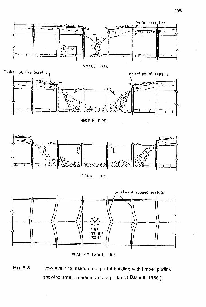
iM

Pnriril nnpy 1km

SMALL FIRE

Timber purlins burning ç SIeel portal sagging

.77

MEDIUM FIRE

LARGE rIPE

Outward sagged portals

PLAN or LARGE FIRE

Fig. 5.8 Low-level fire inside steel portal building with timber purlins

showing small, medium and large fires ( Barnett, 1986 ).

197

CHAPTER SIX Design Example

IFURIE 1ENGUMIEMIRING DRSUGH DIF LOAD-

1BIZAMUNG SUME1 STRUCUUMIE UN A FIIVi

rcIIEY OTYUCIE IB 1 LIflllW

The Ioadbearing frame in a five-storey office

building (Fig. 6.1) consists of simply supported

I-profile steel girders and H-profile steel

columns. The dimensions (internal) of the fire

compartment and the sizes of the openings are

as shown in Figure 6.2.

Complete evacuation of people from the

building in the event of fire cannot be assumed

with absolute certainty.

The scope of this exercise is to check whether the

columns must be provided with fire insulation.

Where necessary the material is chosen and the

insulation thickness required determined.

Fig. 6.1 Five storey office building

55 in 4.0 m

50m I

W. Compartment of Fire Origin 4::x::x::x::x

Roof Load Surface

'

.5m

F L 2.00m

3.5m

150m

3.70m_______

400 m______________

kW1ALIL(S]

External

Internal

surface layers of steel sheeting with

intermediate 100mm mineral wool

steel studs covered on each side with

2*13mm gypsum plaster sheets

Fig. 6.2 Internal dimensions of the fire compartment.

199

200

6.1 BS 5950:Part 8: Code of Practice for Fire Resistant Design

A check is to be made with regard to the central columns as well as the columns

along the facade on the top and bottom storeys.

Here the structure is assumed to have columns in simple construction where the

connections between members are assumed not to develop moments

adversely affecting either the structural members or the structure as a whole.

The distribution of the forces may be determined assuming that members

intersecting at a joint are "pin-ended",

Exam Die Ref.

Roof loading BS 6399: Part 3:19.88

Imposed: 0.60 kN/m 2 (without access)

Dead: 1.20 kN/m2

Factored load: F= 1.4 x 1.2+ 1.6 x 0.60=2.64 kN/m 2

Floor loading

Imposed: 2.50 kN/m2 (offices for general use)

Dead: hx24=0.25 x 24=6.00 kN/m 2

where:Basic span/effective depth ratio = 20

5000/d = 20, d=4000/20=200 mm

Steel 20mm for reinforcement

C30, cover=25mm

Nominal depth of slab = 200 + 10 + 25 =235mm

Assume h = 250mm = 0.25m

Factored load: 1.4 x 6.0+1.6 x 2.5 = 12.40 kN/m2

BS 8110: Parti: 1984 Table 3.11

ExamDle (Continue

SLAB - DISTRIBUTION OF THE LOADING

Every slab in the structure studied is a two-way slab

with I /1 =1.25. The reactions at the middle of the Y

edges of each slab are given below: p1

q-22 (1)

pl y yrm=1 (2)

201

Ref.

BETON KALENDER (1983)

Top level

p=2.64 kN/m2 from equation (1): q=2.64x4.O/2.02=5.23kN/m

from equation (2): q =2.64 x5.0/1 .99=6.63kN/m rm

Bottom level

p=12.40 kN/m2 from equation (1) :q=l 2. 40x4.0/2 .02=24.56kN/m

from equation (2):q =1 2.40x5.0/1 .99=3 1 .1 6kN/m rm

BEAMS

TOP LEVEL

Span 5. Om

Assume 254x1 46x31 U

Design strength p,

T=12.7mm<16mm, p=275N/mm 2

BS 5950: Part 1:1985

t=7.3mm

Ref.

202

ExamDle (Continue

Section class

-Outstand element of compressive flange b

=8.49<1 5e=1 5

e=1

-Web with neutral axis at mid-depth

=35.9<1 20e=1 20

F-= 1

Non slender section

Load 2x5.23+0.31=10.77kN/m

Applied moment M= 10.77x5. 028 =33.66 kNm

Slenderness X - 5000 =149

33.5

Lateral torsional buckling resistance moment Mb=SX Pb

x= D/T = 251.5 / 8.6 =29

AJx=5.10

Buckling parameter

u=0.9 (conservative)

n=1

TABLE 14

for roiled

I-profile

sections

4.3.7.5

for rolled

I-pro file

sections

TABLE 13

203

Ref.

4.3.7.5

TABLE 11

Example (Continue)

xO.82 x149= 110

b=109 N/mm2

Mb=109 x 395.6 x 10-3 = 43.12kNm

Since M=33 .66 kNm< Mb

Section adequate

Span 4. Om

Assume 254x102x28 UB

Design strength

T=10mm<16mm, py=275 N/mm2

t=6.4mm

Section class

- Outstand element. of compressive flange b

5e=15

e=1

- Web with neutral axis at mid-depth d 1=35 . 9< 120

Nkwi slender section

Load 6.63 x 2+0.28 = 13.54 kN/m

Applied moment M-1 3.5<4.02_27 kNm

TABLE 6

ITABLE 7

for semi-

I -compact

I section

204

Example (Continue) Ref.

Slenderness 4000

180

Lateral tortional buckling resistance moment 4.3.7.3.

AJx=6.9

v=0.73 ITABLE 14

for I-pro file

sections

u=0.9 (conservative) 4.3.7.5.

for rolled

I-sections

n=1 TABLE 13

xO.73 xl 80=118.26 4.3.7.5

Pb= 99N/mm2 TABLE 11

Mb=99 x 353.4 10-3=35.0 kNm

Since M=27.0 kNm<Mb

Section adequate

ANY OTHER LEVEL

Span 5.0 m

Assume 406 x 178 x 67 UB I

Design strength p I TABLE 6

T=14.3mm<16mm, P=275N/mm2 I t=8.8mm

205

ExamDle (Continue

Ref.

Section class

-Outstand element of compressive flange b

5e=1 5

E=1 OR

-Web with neutral axis at mid-depth

.0<1 20c=1 20

E=1

Non slender section

ITABLE 7

for semi-

corn pact

sections

Load 24.56 x 2 + 0.67 =49.79kN/m

Applied moment: M_49.798X5.O_l55.59 kNm

Slenderness X5000i 25 40.0

BS 5950:

Part 1: 1985

Lateral torsional buckling resistance moment

14.3. 7.3

x= D/T = 409.4/14.3 = 28.63

A/x=4.5

v=0.84

ITABLE 14

for I-pro file

sections

U=0.9 14.3.7.5

for rolled

I-sections

Example (Continue) IRef.

n=1 TABLE 13

x 0.84 x 125 = 94.5 4.3.7.5

b='34 N/mm2 TABLE 11

Mb=l 34 xl 346 xl =i 80.36 kNm

Since M=155.59 kNm< Mb

Section adequate

Span 4. Om

Assume 406 x 178 x54 UB

Design strength p

T=10.9mm<16mm, p=275N/mm2 TABLE 6

t=7.6mm

Section class

- Outstand element of compressive flange TABLE 7 b ¶=8.15<15c=15 for I-profile

e=1 OR sections

-Web with neutral axis at mid-height

=47.4<1 20e=1 20

F_=1

Non slender section

207

Example (Continue

Ref.

Load 31.16x 2+0.54=62.86 kN/m

Applied moment M_62.868X4.O2 -125.72 kNm

Slenderness A.4°8°5°_1 03.9

r = 'ii 4.3.7.3

v=0.92

u=0.9 (conservative)

n=1

),LT0.9 xO.92 x 103.9=86

Pb=154 N/mm2

Mb=l 54 x 1048 x 10=161 kNm

Since M=125 . 72<Mb

Section adequate

TABLE 14

for 1-pro file

sections

4.3.7.5

for roiled

I -sections

TABLE 13

4.3.7.5

TABLE 11

ExamDle (Continue

COLUMN DESIGN CHECK

Loads

TOP LEVEL

Dead loads - not factored

Floor load 1.20 kN/m 2 qx .20 x 4.0 /2.02 = 2.38 kN/m

q=1 .20 x 5.0 / 1.99= 3.02 kN/m

The reaction at each end of the beam:

Beam with span of 4.Om (3.02+0.28)x4.01 2.64kN

2x 2

Beam with span of 5.Om (2.38+0.31)x5.0 =1 2.68kN

2x 2

Imposed loads - not factored

Floor load 0.60kN/m 2 x =0.60x4.0I2.02=1 .1 9kN/m

rM

q =0.60x5.0/1.99=1.51 kN/m rm

The reaction at each end of a beam:

Beam with span of 4.Om 1.51 x4.0

2x 2 =6.O4kN

Beam with span of 5.Om 1-9x5 ' 0 .95kN 2x 2

11

Ref ExamDle (Continue

Any other level

Dead loads not factored

Floor load 6.OkN/m2 x =60x4•012.02=1 1 .88kN/m

q 'rm

=6.0x5.0/1 .99= 1 5.08kN/m

The reaction at its end of a beam:

Beam with span of 4.Om

(1 5.08+0.54)x4.0 61.4 M2x

2

Beam with span of 5.Om (1 1 .88+0.67)x5.0 61 .O8kN

2x 2

Imposed loads-not factored

Floor load 2.5kN/m2

qx 5x4.0/2.02=4.95kN/m rM

q =2.5x 5.0 /1 .99=6.28kN/m nfl

list II.]iI.kt..i1,t.EFi.I*iIl!

Beam with span of 4.0m

2x 6.28x4.02512 kN

2

Beam with span of 5.Om

2x 4.95x5.02475 kN

2

209

210

ExamDle (Continue Ref.

6.1.1. Centre Column

TOP LEVEL

Design In ambient environment

Design load

F = 1 .4x2x(1 2.64 + 12.68 ) + 1 .6x2x (6.04 + 5.95 )+1.4x

(0.23x3) = 110.23 kN

Assume 152 x152 x23 UC

Design strength p

T=6.8 mm < 16 mm, p=275 N/mm 2

Table 6

t=6.1 mm

-Outstand element of compression flange

Table 7

=11.2<15c=15

for semi-

El compact

sections

-Web generally

20.2

R=_c= 110.23 xlO =0.14<0.5, positive

Py 29.8 x275

d 120e=98.0 t51 +1.6R

3.5.4

ExamDle (Continue

-Web subject to compression throughout

=12.4<39e =39

Section adequate

Effective length LE = 0.85 L

3.OxO.85x1 0 2 Slenderness X= 3.68 = 69.29

Check for compression

Compressive strength

H-section and for thickness _<40 mm, 27c

For ?.=69.29 and p=275 N/mm 2

= 183 N/mm2

211

Ref.

Table 7

for semi-

compact

sections

I Table 25

I Table 27c

for yy axis

of buckling

Compressive resistance

PC = A PC = 29.8 xl 83 xl 01 = 545.34 kN

Since, PC = 545 kN> FC

4.7.4

for plastic,

compact,

semi-

compact

sections

212

Example (Continue

Ref.

The following relationship must be satisfied:

F Mx * M +-

A9 p,, --

where: F= 115.70 kN

Ag=298 cm2

275 N/mm2

M= M =0

F 11"23 xl

So, C - O=0.14<1 A 9 P 29.8x275

Section adequate

14.8.3.2

14. 7. 6(3)

1N..xA1tilI1!tl1iT]

14.7.7

The requirements for overall buckling will be satisfied in this

context by the "Simplified approach" (nominal moments applied).

F M M C X X

PC Ir

z bs y y 14.8.3.3.1

where: FC 110.23 kN

IVIX = M =0

A = 29.8cm2

P=183 N/mm2

m=1 F 110.23

So, A = 10=014<1 9 C 29.8 x275

Section adequate

213

Ref.

BS 5950:

Part 8:1990

ExamDle (Continue

Design in a fire environment

Assume that the whole imposed load is non-permanent

F= 1 .0 x2 x(1 2.64 + 12.68 ) + 0.8 x2 x(6.04 + 5.95) + 1.0 x

(0.23 x3.0 ) = 70.51 kN

70.51 A = 29.8 183

xl 0 = 0.13 < 0.2, Ag=29.8cm2. p=183N/mm2

Limiting temperature

?= 69.29<70

eL = 71 0°C

4.4.2.3

Table 5

Design temperature

Case 1. Column exposed from four sides.

For flange thickness = 6.8 mm

For fire resistance period of 90 mm, 1006°C



So, 0D >

Protection required

I Table 6

Case 2. Column built next to a wall

For flange thickness 6.8 mm




I Table 7

ExamDle (Continue

MA Protection required

The design temperatures derived from Table 7 refer to beams

and generally to heating from three sides. Because the furnace

for beams has different thermo-properties than the one for

columns, the values above may be slightly different from the

ones if the table referred to columns.

Because of the large temperature gradients developed, more

exact method of calculation has to be used.

BOTTOM LEVEL

Design in ambient temperature

Design load

F= 1 .4x2x{(1 2.64+1 2.68)+(61 .4+61 .08)x4}+1 .6x0.6x2

x{(6.04+5.95)+(25.12+24.75) x4}+1 .4x{(O.86x3.5)+

+(0.23 x3.0) x4}=1856.77 kN

Assume 203x203x86 UC

Design strength p,

For T=20.5mm and t=13.Omm

Because T>16mm and 1<40mm, p=265N/mm 2 TABLE 6

214

ExamDle (Continue

Section class

-Outstand element of compression flange

=5.09 <15e=15.30

c=(275/p) 1 =1 .02

TABLE 7

for semi-

compact

sections

215

-Web generally

12.4

Fc 1856.77 R=-=

110 . 1 265xlO=O.64>0.5, positive

12.4=t (93-54R)c=58

OR

-Web subject to compression throughout

2.4< 39e=39.78

Non sender sec t ion

Check for compression

Effective length LE=0. 85 L

3.5x 0.85 xlO Slenderness A.- 5.32

2_55.92

A<180 max slenderness for members

resisting loads other than wind loads

H - section and for thickness ! ~ 40 mm, Table 27c

3.5.4

TABLE 7

I for semi-

I compact

I sections

4.7.2

4.7.3

4.7.3.2

Table 25

14 ExamDle (Continue

M= the moment capacity about the major axis in the

absence of axial load

M=the moment capacity about the minor axis in the

absence of axial load F 1856.77

So, C = x10=0.64<1 A9p 110.1 x265

®©©ET sd@qu&R@

The requirements for overall buckling will be satisfied in this

context by the "Simplified Approach" (nominal moments applied):

F M my y<1O

AgPc MbS PyZy -

where :F=1 856.77kN

M=M= 0, the loads are balanced about the xx and yy axis.

Ag=llO•l cm2

P=202 N/mm2

m=equivalent uniform moment factor=1 F 185677

So, C - xl 0=0.84<1 AgPc 110.1x202

216

4.7.7

14.8.3.3.1

217

Example (Continue) Ref.

Compressive strength For A=55.92 and p=265 N/mm 2 ,

P=2O2NImm2

TABLE 27c

for yy axis

of buckling

Compression resistance

P=A9 p= 110.1 x202x101=2224kN 4.7.4

Since, P>Fc, for plastic,

compact,

Section adequate semi-

compact

For axially loaded compression members with moments sections

separate checks are required for local capacity and overall

buckling.

Check for local buckling

The following relationship must be satisfied:

F M M

Ag Py 4.8.3.2

where:F =1856.77 kN

Ag 1 10.1cm2

Py 265 N/mm2

M=M=O 4.7.6 (3)

218

Ref.

BS 5950:

Part 8:1990

ExamDle (Continue

Design In a fire environment

Assume that the whole imposed load is non-permanent

F= 1.0 x2 [(12.64 + 12.68) +(61.4 + 61.08 )x4]+

0.8 xO.6 x2 x[(6.04 + 5.95) + (25.12 + 24.75 ) x4] +

1.0'[ ( 0.23 x3.5 ) + (0.86 x3.0 ) x4]= 1239.26 M.

Load ratio Ff M X

R=A g pMp Z,

where:

Ag = gross area;

p=compressive strength;

p=design strength of steel;

z=elastic modulus about the minor axis;

M=buckling resistance moment (lateral torsional);

F1 = axial load at the fire limit state;

M1 =max moment about the major axisat the fire limit state;

M= max moment about the minor axis at the fire limit state.

14.4.2.3

1239.26 So, R= x1O=0.56

110.1 x202


=55.92<7O and R=0.56

0L 560°C I Table 5

Example (Continue

Design temperature

Case 1 :Column exposed from four sides

For flange thickness 20.5 mm and

for fire resistance period of 90 mm, 0=950°C


for fire resistance period of 30 mm, 0=661 °C

So, 0D>°L'

Protection required

Table 7

Case 2: Column exposed from three sides

For flange thickness 20.5 mm and




So, 0D>0L'

Protection required

The design temperatures derived form Table 7 refer to beams.

Because the furnace for beams has different thermo-properties

than the one for columns, the values above may be slightly

from the the ones if the Table referred to columns.


exact method of calculation has to be used.

Table 7

219

220

ExamDle (Continue

Ref.

6.1.2 Edge Column

TOP LEVEL

Design In ambient environment

Span 5. Om Load=1 0.77kNm

Assume 254 x 146 x 31 UB

Check as for centre columns

Span 4. Om

Assume 254 x 102 x 22 UB

Design strength p Table 6

T=6.8mm<16mm p=275 N/mm 2

Grade 43

t=5.8mm

- Outstand element of compressive flange

=7.47, <15E=15

E=1

- Web with neutral axis at mid-depth

=38.8<1 20

Non slender sect©n

Table 7

for semi-

compact

sections

Load

6.63+0.22=6.85kN/m

Applied Moment

Slenderness

M= 6.85x4.02

_13.7

4000 20.5--1 95.12

221

Example (Continue

IJ

Lateral torsional buckling resistance moment

4.3.7.3

x= DTF=254/6.8=37.35

AJx=5.22, N=0.5

Table 14

Slenderness factor v=0.81

for I-pro file

sections

u = 0.9 (conservative)

4.3.7.5

or rolled- -

sections

n=1

x 0.81 x 195.12 = 142.24

pb=73N1mm

Mb=73 x 261.9 x 10 3=19.12kNm

Since Mb>M

Section adequate

Table 13

4.3.7.5

Table 11

Any other level

Span 5.0 m Load=49.79kN/m

Assume 406x 178 x67UB


Span 4.Om

Design strength p,

T=14.3mm<16mm p,=275 N/mm2

t=8.8mm

I Table 6

Example (Continue

Ref.

Section Class

.iwmr S

- Web with neutral axis at mid-depth

p=:41.0<1 20

Load :31 .16+0.39=31.55 kN/m

Applied moment: M=-1-558 x4.02

=63.10 kNm

Slenderness 404000 =100

Table 7

for semi-

compact

sections

4.3.7.3.

I'll

Y4cWj'

Slenderness factor v=0.91

Buckling parameter u = 0.9 (conservative)

n=1

X 0.91 xl 00=81.90

Pb='595° N/mm2

Mb= 1 59 . 50x 1346 x 10=214.69 kNm

Since Mb>M

Section adequate

Table 14

for I-pro file

sections

4.3.7.5

Table 13

4.3.7.5

Table 11

223

Example (Continue

Re

COLUMNS

TOP LEVEL

Design in ambient environment

Design load

F C = 1.4 x ( 2 x 6.48+12.68)+

+1 .6x(2x3.02+5.95)+1 .4x(O.23x3)=56.O5kN

Eccentricity of connections

e=1 52.4/2+1 00=1 76.2mm 4.7.6(3)

e=6. 1/2+100=103.05mm

Nominal moments

M x=(l .4x1 2.68+1 .6x5.95)x1 76.2x1 0-3 =4.81 kNm

The loads are balancebout the y-y axis, M ey=O

Design strength

p=275N/mm2

Section class


Non slender section

I Table 6

14.8.3.2

F A9p7Mcx+M cy -

56.05 4.84 = + =0.10<1

29.8x275 275x1 84.3x1 0

Section adequate

ExamDle (Continue

224

FC Mx M

A <1 gPc b P yy

where .A.LT=O.85 L/r=0.85x300/3.68=69.29

Pb=1 88N/mm2

56.05 4.84 So + =0.15<1

29.8x275 188x184.3x10 3

Section equate


Design load

Fc 1 .Ox(2x6.48+1 2.68)+O.8x(2x3.02+5.95)+1 .Ox(0.23x3)

=35.92kN

4.8.3.3.1

Table 11

lBS 5950:

IPart 8:1990

Nominal moments

Mt=(l .Oxl 2.68+0.8x5.95)xl 76.2x1 0 3=3.07kNm

Load ratio F1 M1

R=AgPc+Mb+PyZy M=0 fy

14.4.2.3

35.92 3.07 =0.10

29.8x1 831 88x1 84.3x1 0


A=69.29<70 and R=0.10, eL= 71 oc I Table 5

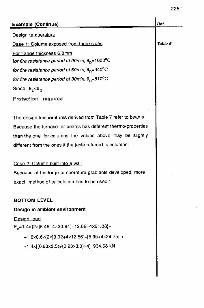
ExamDle (Continue

225

Design temperature

Case 1: Column exposed from three sides

For flange thickness 6.8mm

for fire resistance period of 90mm, 9D=1 000°C

for fire resistance period of 60mm, OD=940°C

for fire resistance period of 30mm, 0D=81 0°C

Since, 8 L<OD

Protection required

The design temperatures derived from Table 7 refer to beams.

Because the furnace for beams has different thermo-properties

than the one for columns, the values above may be slightly

different from the ones if the table referred to columns.

Case 2: Column built into a wall


exact method of calculation has to be used:

BOTTOM LEVEL


Design load

F= 1 .4x{2x[6.48+4x30.94]+1 2.68+4x61 .08}+

+1 .6x0.6x{2x[3.02+4x1 2.56]+[5.95+4x24.75]}+

+1 .4x[(0.68x3.5)+(0.23x3.0)x4]=934.68 kN

Table 6

ExamDle (Continue

Eccentricity of connections

e=21 1.15mm

e=1 06.5mm

M=(1 .4 x 61.08 +1.6 x24.75 ) x ex X1 0-3 =26.42 kNm

The loads are balanced about the y-y axis Mey=O

Design strength

p=265 N/mm2

Table 6


FC M M < A9p + M MCY

where: F =934.68 kN C

M=pS=265x978.8x1 0 -3=259.38kNm

So 934.68 26.42

110.1x265 259-38

14.8.3.2

226

227

ExamDle (Continue

Ref.

F M M Agpc+ &, M +pyzy~ l

where: F =1 01 3.83kN C

O.85L 0 .85x350 k1= r = 5.32 =55.92

Pb=219 N/mm2

M=21 9x978.8x1 0=21 4.36kNm

934.68 26.42g

Therefore, xl O+ 594 110.1x202

8=0.52<1


Design load

F= 1 .Ox{2[6.48+30.94x4]+1 2.68+61 .08x4}+

0.8x0.6{2[3. 02+1 2.56x4]+[5.95+24.75x4]}+

1 .0[(0.86x3.5)+(0.23x3.0) x4]=624.1 3kN

4.8.3.3.1

Table 11

lBS 5950:

IPart 8:1990

gel

1 4.4.2.3 Ff M Mf

R=Ag

where :Ff=624. 13 kN

Ag=l101 cm2

p=202 N/mm2

le (Continue

MfX=(l .0x61 .O8+O.8x24.75)ex1 O=i 7.08kNm

0.5L 0.5x350 LT r = 5.32

Pb=265 N/mm2

MbS=265x978. 8x 1 0=259.38 kNm 624.13 17.08

Therefore, R= xl 0+259 38=0 . 346 110.1x202


For A.=55.90<70 and R=0.34, 8 L=640°C Table 5

Design temperature

Case 1 :Column exoosed from three sides

For flange thickness 14.3mm and

for fire resistance period of 90mm, 9 0=950°C

for fire resistance period of 60mm, 9 0=877°C

for fire resistance period of 30mm, OD_709 C

Since, 8L<eD

Protection required

The design temperatures derived from Table 7

refer to beams. Because the furnace for beams

has different thermo-properties than the one for

columns, the values above may be slightly

different from the ones if the table referred to columns.

Table 6

228

230

Examole (Continue) IRet

6.2 European Recommendations for the Fire fEur3,

Safety of Steel Structures iggoj

6.2.1Centre Column

BOTTOM LEVEL


203 x 203 x 86 UC

Fc= 1856 . 77kN

Fe 430

t-<40 a=275N/mm2 Table 1

Section classification - Plastic section (Category 1) Appendix B

-Web subject to compression d =

160.8 = 12.37<33E = 30.36 13.0 Table 3

Sheet 1

section

class 1

Appendix B

-Outstand Flange subject to compression

= °85 e =5.09<10= 9.20 Table 3

Sheet 3

section

class 1-

-roiled

sections

Appendix B

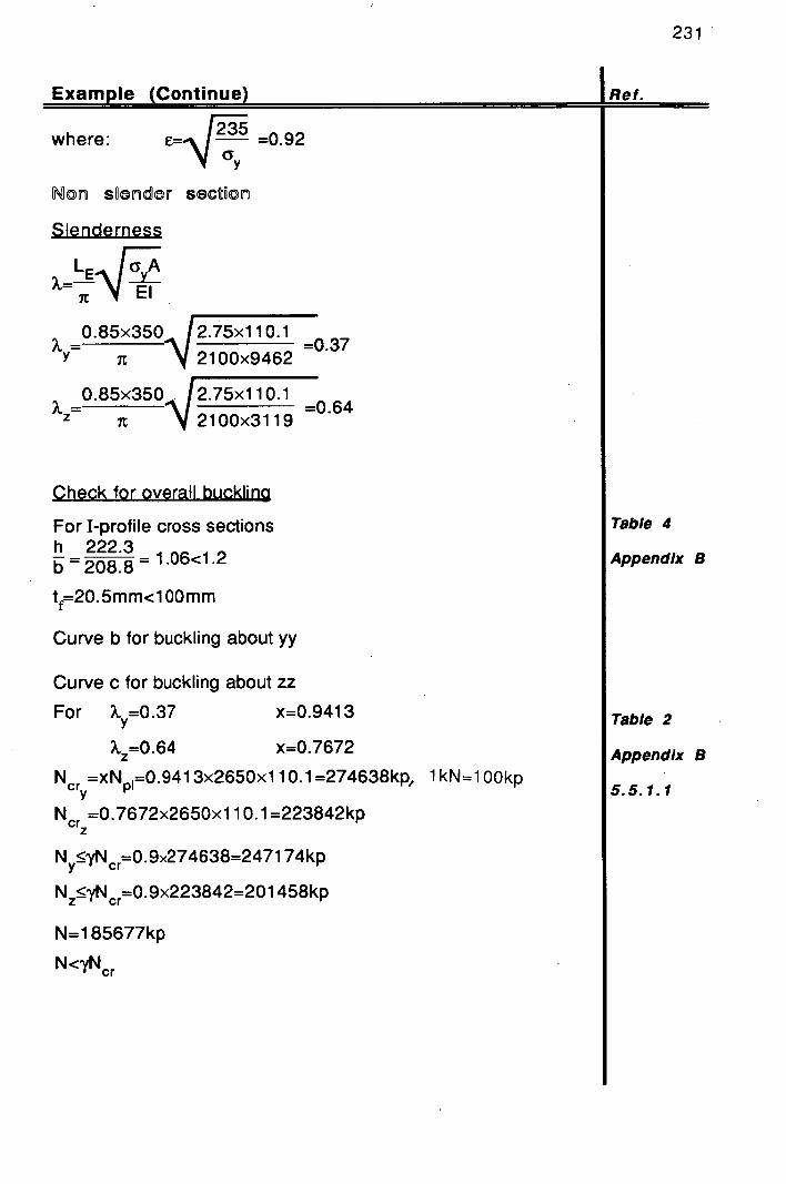
231

ExamDle Continue)

f.

where: c=.J 5 =0.92

Non sOenftr section

Slenderness

7r VEJ

0.85x3502.75x1

10. 1 Y it 2100x9462 =0.37

0.85x350 75X1 10.1 Z _\[2 =0.64

For I-profile cross sections h 222.3

1.06<1.2 b208.8 =

tf=20.5mm<l 00mm

Curve b for buckling about yy

Curve c for buckling about zz

For ?=0.37 x=0.9413

=0 . 64 x=0.7672

Ncr =xN =0.9413x2650x1 10.1=274638kp, lkN=lOOkp y P

Nc =0.7672x2650x1 10.1=223842kp

N y:!~?Ncr=O. 9x274638=247 l 74kp

N z:!~'/N cr=09X223842=201 458kp

N=1 85677kp

I Table 4

IAppendlx B

I Table 2

I Appendix B

15.5.1.1

N<YNcr

232

Examole (Continue) - IRe!.

Section adequate

Section factor 2h+4b-2d

IIv=croSS sectional area

2x22.23+4x20.88-2x1 .1 4cm 1 = 110.1

=1.1 4cm -1 =1 14m 1


for fire resistance period of 90mm

Temperature of steel column O=998°C

Corresponding yield stress

O s

°yO 1081 1000 141= =

Gy 20

O-440 =0.00039

ay eN'y 20=0.00039x265=0.1 ON/mm 2

P=201 458kp

P 9=P

9

=201458x0.00039=78.57kp U Uaa

(ECCS,

1983)

Table 5

Appendix B

2.3.3

233

ExamDle (Continue

f.

Correction factor k=0.85

Admissible load under fire conditions

Pu0 =92.44kp

Since P<N= 1239kN

PROTECTOON REQUDRED

5.4.3


Table 5

Temperature of steel column 0=932°C

Appendix B


iji=0.01 493

G ye

96N/mm2

Buckling load at the temperature 932°Q

P 9=201 458x0.01 493 = 300 8k

Since P 0<N

POTECTDON REQUMED

2.3.3


Temperature of steel column 0=790°C

I Table 5

IAppendIx B


'v=O .06480

12.3.3

ye =17.17N/mm2

234

ExamDle (Continue) IRef.

Buckling load at the temperature 790 0Q

1 9=1 3054kp

Since P 0<N

PROTECTMN IREQUORED

TOP LEVEL fEur3,

Design in ambient environment iggoj

152 x 152 x 23 UC,

F =110.23kN C -

Fe 430

t!!~40 a=275N/mm2 Table 1

Appendix B

Section classification (Category 3)

-Web subject to compression Table 3 d = 123.4

= 20.23 < 33e = 30.36 Sheet 1

section

class 1

Appendix B

-Outstand flange subject to compression Table 3

I h 1 .21<1513.80 Sheet 3

Non slender section section

class 1

Appendix B

ExamDle (Continue

Slenderness

____ .75x29.8 LE ____

El 2_________

= 0.45 S 263

0.85x3004?

2j

.75x29;8 080

IC 00x403

Check for overall buckling h 152.4

1 52.4=1<1.

t=6.8mm<l 00mm

Curve b for buckling about yy

Curve c for buckling about zz

For ?=0.45 1x=0.905

For ?=0 .80 x=0.662

Ncr = xN 1 = 0.905x2750x29.8 =74164.75kp

Ncrz = 0.662x2750x29.8 = 54250.90kp

N:5 YNcr = 0.9x74164.75 = 66748.28kp

N ~5 cr =0.9x54250.90=48825.81 kp

N=1 1 023kp

N<YN cr

Sector adequate

Section factor

FN=30.27 m 1

235

Ref.

Table 4

Appendix B

Table 2

Appendix B

5.5.1.1

236

ExamDle (Continue

Ref.


ECCS,


19831

Temperature of steel column

Table 5

e=954°C

Appendix B


108 (1 954i000

IV=954-440 = 0.00967

CY y = lii c 20=0.00967x 275=2.66N/mm 2

2.3.3.

Buckling load at the temperature 954

P=4971 3kp

Pue = P ---=49713 x.00967=48.07kp

Correction factor k=0.85

Admissible load under fire conditions

P=48. 07/0.85=56.55kp

N=7051 kp>56.55kp

Protection required

15.4.3

237

Ref. ExamDle (Continue

or fire resistance penod of 60mm

Temperature of steel column O=81 4°C


ljJ=O.O 5371

4.77N/mm 2

Buckling load at the temperature 0=814 0Q

P 0=267Okp

Since P0<N=7051 kp

[t1tII[®]IiiI(.1Ii1IEfl]

for fire resistance of 30mm Temperature of steel column e=484°C


'41=1.27

Table 5

Appendix B

2.3.3

I Table 5

Appendix B

2.3.3

Buckling load at the temperature O= 484°C

P=62964/0 . 85=74075kp

Since P 0>N=7051 kp

No pr©Vco1 raqufre

238

6.3 Swedish Institute of Steel Construction

Fire Load and Opening Factor

Compartent size = (4.0x3.5 x2.5) m 3

Construction: Dense concrete

Fire Load

From Table 2 [Appendix C] the design fire load is equal to 33.0 Mcal / m 2. This

value applies only to the fire load due to furniture and fittings.

The load due to floor and wall coverings can be derived from the following

equation.

flyç, (Mcal / m2) (MJ / m2) (6.1)

where: m= the total weight of each individual combustible material

constituent v in the fire compartment (kg).

H= the effective calorific value of each individual combustible

material constituent v in the fire compartment. (Mcal / kg ) {MJ / KG}

A= the total interval surface area of the fire compartment (walls,

floor, ceiling) (m 2)

Assumptions

-weight of floor covering

1.5( kg / m2)x(4.0x3.5) (m 2) =21.0 m2 (6.2)

-calorific value of floor covering : 5.0 (Mcal / kg)

-weight of wall covering

0.2 (kg / m2)x2.5 m2 = 5.0 kg (6.3)

-calorific value of wall covering : 5.0 (Mcal / kg)

From the above:

239

m (kg) H,, (Mcal / kg) m, H., (Meal)

Floor covering 21.0 5 105.0

Wall covering 15.0 15 125.0

lmvHv = 130.0(Mcal)

At =2x(3.5x 2.5 )+2x(4.0 x3.5 )+2x(4.0 x2.5)=65.5m 2

From Equation 6.1 the fire load

130 Mcal q=(655)(

m2 f2 -)=1.98=2.00 (Mcal I m 2)

Total Design Fire Load: 33.0+2.0=35.0 (Mcal / m2)

Opening Factor ( A[ii7A t )

1/ Door closed (It remains intact during the fire)

A = ventilation area =( 3.7 x 1.5) (m2) = 5.55 m2

h= 1.5 m

At = 65.5

Af}h - 5.55 TiT = 0.104 rn"2 = 0.105 mU2 At - 65.5

A = 5.55 + (2.0 x 1.0 ) = 7.55 m

ATh - 7.55-[iT =0.141 m 1/2 = 0.15 m 1/2 A - 65.5

240

For centre columns, the opening factor will be taken into account as equal to

0.15 m 112 to cover every possible case (door closed , open or intact during the

fire).

For columns across the facade, the opening factor will be taken into account as

equal to 0.105 m 1/2 to give results on the safe side.

3. Equivalent Fire Load and Opening Factor

DATA Material Area

Floor and Roof Concrete 2x(3.5x4.0 )=28 (49%)

Wall Gypsum plaster 2 x 2.5 x 3.5 + 2.5 x 4.0

-1.0 x 2.0 =

= 25.5 (44.0%)

Steel Sheeting 4.0 x 2.5 - 3.7x 1.5 =

with 4.40 (7%)

mineral wool insulation

The fire compartment is a combination of the materials below:

Fire Compartment Type B Concrete (100%)

Fire Compartment Type G Concrete (20%)

2 13 mm gypsum plaster - board

loomm air gap }80%

2 13 mm gypsum plaster board

Fire Compartment Type H Steel Sheeting

100 mm mineral wool } 100%

Steel Sheeting

241

According to the above fire compartmment:

__ 44 k- - ...!

kII(B)+1 OO)+ lOOkf() (6.4)

100 -

a/ for opening factor AJii 105 rn 1 ' 2 and from Table 3 [Appendix C] At

kf =0.85

kf = 2.875 = 2.88

=1.125 = 1.13

kfØ2Ø (B) (6.5) =0.80kf +0.20kf kf

(G) (P) (p) 0.80

From equations (6.4) and (6.5):

kf = 1 0.85 +2.88 + () ()1.13 - ()() 0.85 = 1.14

b/ for Opening Factor A 11i At

kf0 85

k1 .20Ø

kf090

(G) 0 .20 kf

(B) (6.6) 0.80 k +0.20 kf f(p) (B) k (P) = 0.80

From Equations (6.4) and (6.6):

kf= 49 7 44 '1 20

0.85 + 2.00 + 0.90 - ()() 0.83 = 0.96

Equivalent Fire Load = kf x actual fire load

242

- for opening factor Ah

=0.105 rn 2 At

q= 1. 14 x 21.5 = 24.50 (McaVm2 )

k1 =1.14

- for opening factor = 0.15 m 2 At

q=0.96x21.5=20.6(McaI/m2)

k-0.96

Equivalent Opening Factor = k f xactual opening factor

- for opening factor Ah

= 0.105 rn 1"2 At

AJh =1.14x0.105=0.12m 2 At

kf= 1.14

-for opening factor Ah

= 0.15 m 2 At

AJh At = 0.96 x 0.15 =0.14 rn'2

krO.96

Maximum Steel Temperature

Centre Column

Case 1: Exposed from four sides

Resultant emissivity

For type of construction 1 - column exposed to fire on all sides and from Table 4,

the resultant emissivity Cr 0.7

The accurate value for emissivity is given below:

243

1 Er- 1 =0.7

—+---1 Ct Cs

where: Et = emissivity of the flames = 0.85

CS = emissivity of the steel section = 0.80

F ratio

—s FS 2h+4b-2d VS — cross sectional area

Top storey 152x1 52x23 UC

Fs 2x152.4+2x152.4-2x6.1 = 0.3109 Mm -1 =311 m4 29.8x102

Bottom storey 203x203x86UC

F5 2x222.3+2x208.8-2x13011388 mm 4 = 113.88 m4 = 114 m4 110.1x102

Maximum steel temperatureOm

Equivalent Fire Load

Equivalent Opening Factor

Resultant Emissivity F 5

VS

=3360 {Mcal / m2 }=34 {Mcal / m2 )

=0.14 m 1

=0.7

=114 m 1 (bottom)

=311 m' (top)

F/VS and A-[/A values are out of the range of Table 6.

For a given resultant emissivity and opening factor, the maximum steel

temperature increases with an increase of the ratio F5/V 5 .

For a given resultant emissivity and a given F5/V 5 ratio, the maximum steel

temperature decreases with an increase of the opening factor.

So, 0>770°C

This value is out of the range of temperature values of Figure 5.

244

Top storey

For a s=2600 kgf / cm2 {260 MPa} ,y=l, ?=69.29 and from Table 5, ak< 55

MPa, P<55x29.8x1 0-1=1 63.9kN

P=70.51kN<163.9kN

O PROTEMON REOtUORED

Bottom storey

For (=2600kgf/cm 2{260MPa}, y=1, A=56 and from Table 5, akcz62 MPa,

P<62x110.1x10 1 =682.6 kN

P=1 239kN> 682.6kN

PROTECTMN REQUORED

Case 2: Next to a wall


Cr=O 7 (to obtain steel temperatures on the safe side)

ELL ratio

FS 2h+3b-2d Vcross sectional area

Top storey 152x1 52x23 UC, F 2x1 52.4+3x1 52.4+2x6. i=O 251 6mm

1 =251 m 1 V s 29.8x102

Bottom storey 203x203x86 UC, F 5 2x222.3+3x208.8-2x1 3 =0.09491 mm

1 =95m 1 V S 110.1x102

Max steel temperature 9 iiax

q>770°C

Out of the range of Figure 5

For =260 MPa, y=1 we conclude the following:

Top storey

For X=69.29, a k<55MPa, P=70.51 kN<1 63.9kN

P-Mi

For X=56, P=1239.26kN>682.6kN

Column built into a w


r E& ratio

FS b 1 V = bt = t

Top storey 152x152x23 UC,

vs ===O.147mm1 =147m -1

Bottom storey 203x203x86 UC,

= = 20.5 = 0.049mm = 48m

Max steel teniperatureO 1

emax>54o°C

Criticalbucklingstress

Topstorey

For G=260MPa, y=l , Omax=600°C , ?=69 and Fig.5, Gk=50MPa

P=50x 29.8 x10 1 =149kN>70.51kN

O PROTECTMN REQUMED

Bottomstorey

For cY=260MPa, y=l , Omax=540°C , ?=56 and from Fig. 5, a k=85MPa

P=85x1 10.1x101=935.9kN<1239.26kN

245

Edge column

Case 1: Next to a wall

Resultant emissivity, FSNS ratio, Omax as for Centre Column design, Case 2.

Too storey

P=35.92kN<1 63.9kN

O PROTECTOON REQUOED

Bottom storey

P=624kN<682.6kN

O PROTECTMN REQUDRED


Resultant emissivity, F sNS ratio, Omax as for Centre Column design, Case 3.

Top storey

P=1 49kN>35.92kN

O PROTEMON REQURED

Bottom storey

P=935.9kN>624.1 3kN

O PROTECTMN REQUDRED

246

247

6.4. Fire Protection Insulation

The fire protection insulation VULTEX is chosen from the yellow book

[ASFPCM,'88]. The characteristics of the above material are given in the

Appendix D. The profile protection technique is chosen.

Centre Column

TOP STOREY

FN=3 1 l m 1

for fire resistance period of 30mm, fire protection thickness of 10mm,


for fire resistance period of 90mm, fire protection thickness of 25mm.

BOTTOM STOREY

FN= 1 14m -1

for fire resistance period of 30mm , fire protection thickness of 10mm,



Edge Column

CASE 1

TOP LEVEL

F/V=25 1m 1




BOTTOM LEVEL

FN=95m 1



for fire resisatnce period of 90mm, fire resistance thickness of 22mm.

CASE 2

TOP STOREY

FN=1 47m 1




BOTTOM LEVEL.

F/V=48m 1




248

249

6.5 Conclusions

The results of the fire insulation check are presented in the Tables 6.1, 6.2.

According to those results, one may observe that consideration of the effect of

natural fires can result in considerable benefit. In this context, natural fires are

considered as the fires which build up and decay in accordance with the mass

and energy balance within the compartment. The results obtained if one applies

the British Code, BS 5950: Part 8 [ BSI, 1990 ] and the European

Recommendations[ECCS, 1983] are conservative in comparison with the

Swedish Code results.

In the case of bare columns, which is the object of this study, the fire test results

may not be representative because of the limited series of fire tests contacted.

The test data on columns relates to slenderness values which are less than 50

because of the restraint of the test furnace. In BS 5950: Part 8 [BSI, 1990], the

limiting temperatures for design have been extended up to the slenderness

value of 70 and they are derived by assuming uniform heating on all the faces.

In the design example, presented in this Chapter, the edge column was

designed using limiting temperatures and assuming that the column is uniformly

heated.

Because BS5950: Part 8 [BSI, 1990] applies only to members which are not

subject to second order effects resulting from deflection during a fire, the design

of the Column built into a wall requires the use of a more exact method of

calculation. Because the design according to the European Recommendations

[ECCS, 1983] is limited to individual elements subjected to the standard fire, the

design of a Column next to a wall or built into a wall is excluded.

Further refinement and sensitivity can be offered with the application of finite

element analysis.

250

Code BS 5950: Part 8: European Swedish

Code of Practice Recommendation Institute

for Fire Resistant for Fire Safety of of Steel

Design Steel Structures Constr.

©®i cmuUnh

Cases Fire resistance period

of study (mm)

90 60 30 190 60 30

Top level

Case 1 Yes Yes Yes Yes Yes No No

Case 2 Yes Yes Yes - - - No

Case - - - - - - No

Bottom level

Case 1 Yes Yes Yes Yes Yes Yes Yes

Case 2 Yes Yes Yes - - - Yes

Case 3 - - - - - - Yes

where:

Case 1: Column exposed from four sides

Case 2: Column next to a wall


Yes: Protection required

No: No protection required

Table 6.1 Tabulated results of fire insulation check-

-Centre Column

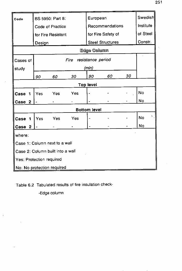
251

Code BS 5950: Part 8: European Swedish

Code of Practice Recommendations Institute

for Fire Resistant for Fire Safety of of Steel

Design Steel Structures Constr.

Ilj

Cases of Fire resistance period

study (mm)

1 90 60 30 190 60 30

Top level

Case 1 Yes Yes Yes - - - No

Case - - - - - - No

Bottom level

Case 1 Yes Yes Yes - - - No '

Case - - - - - - No

where:

Case 1: Column next to a wall


Yes: Protection required

No: No protection required

Table 6.2 Tabulated results of fire insulation check-

-Edge column

252

CHAPTER SEVEN Conclusions -

-Suggestions for future work

Three basic components have been considered in order to predict field

performance and ultimately design a structure for the impact of fire. The

components are given as follows:

the fire

the heat transfer to the structural members

the effect of elevated temperatures on structural performance.

These three components are not independent, but interelate in a very

complex manner. Each involves many parameters. An understanding of

these parameters is necessary in order to develop models which will

adequately predict the phenomenon.

In order to illustrate the interelationships between the three basic

components affecting structural response and identify some of the key

variables in each component, a logic flow chart has been developed for the

response of structural steel to fire (Fig. 7.1). The chart identifies the critical

components necessary to predict the performance of a structural system.

The inter-relations among the three major components are different for each

material. In this study on steel columns, the fire was isolated from the other

two basic components (heat transfer, structural response). It was implied that

the steel structures exhibit a minimum effect on the relationship between the

fire, the heat transfer to structural members and structural response. This

assumption does not hold for structures constructed from different materials.

With regard to wood structures, once wood reaches its ignition point the

wood ignites and augments the original fire. The increased compartment

combustion rate results in an increase in the radiant heat to the wood

253

HEAT TRANSFER STEEL TEMPERATURE S

UNPROTECTED STEEL

COMPUTER MODEL TASEF 2

MATERIAL PROPERTIES thermal conductivity specific volumetric

enthalpy

/\

(_HEAT TRANSFER I

FIRE GROWTH

STANDARD FURNACE TESTS

NATURAL FIRES I FULL SCALE TESTS

GEOMETRY

Fig. 7.1 Components necessary to predict the structural performance

of a structural system.

254

structure and increases the wood charring rate. A reinforced concrete wall

may have an important impact on the heat transfer to and from the

compartment resulting in alterations to a compartment fire.

For the purpose of the present study, the fire growth was predicted either

using the standard fire curve [BSI, 1972] or temperature-time curves for

different fire loads and opening factors [Pettersson, 1970]. Full-scale test

results have also been used as data to predict the structural response to

fire.

The fire environment may also be predicted using computer models. Some

computer models deal only with one phase of fire development, either the

pre-flashover regime or the post-flashover regime. Modelling the pre-

flashover regime is difficult because the details of fuel type and arrangement

are unknown to the designer. To tackle the problem, an envelope of

statistical data derived from a large number of full-scale tests or a series of

computer simulations may be used. Problems regarding the modelling of the

post-flashover fire are similar. If the pre-flashover fire is ignored, flashover is

not predicted and the model may not be applicable to the given problem.

The effect of the preflashover regime on openings into the compartment is

unknown. Window glass breakage and door burn through can be taken into

account. The usual approach to the problem is to assume that all potential

openings into the compartment are open. The reliability of the above

approach is unknown when predicting the development of the real fire.

The second component studied, once the fire is defined, is the heat transfer

to-the structure. This study is limited to structural steel and more specifically

to unprotected steel. The problem at this stage is solved with the aid of the

computer program TASEF-2 which uses a forward difference time approach

(Chapter 3). The material properties used as data to the program are given

255

as a function of temperature (Chapter 2). For the cases studied in this

research, the results obtained compare satisfactorily with those obtained

from the experimental tests (standard or full-scale fire tests). It can therefore

be claimed that the computer program can be used to simulate a standard

test or full scale test conditions.

One of the future trends regarding this program in particular is its

modification to handle three dimensions.

Regarding the present version of the program, the program could be

transformed to model a structural member in a more user friendly way. At the

moment, the user has to model a specific element as a rectangular one and

define areas which are fictitious.

Once the heat transfer problem was solved and the time-dependent

temperature gradient in a structural member was determined, the third

component which is the structural response was studied. In Chapter Five

different design methods have been studied to establish their reliability in

predicting the structural response in a fire. Different design methods were

applied to four column cases and their relative applicability was examined. A

computer model could be used to analyse the effect of fire on the structure.

The analysis should include the effects:

-change in loading

-change in the resistance to the load

The change in load occurs in a structural element because of its restraint to

expansion when heated. It is a serious problem where there are significant

transverse gradients which result in moments in excess of those caused by

the eccentricity of the actual member. Increased temperature causes a

reduction in the structural load resistance of a structural member because of

changes in the steel properties.

256

In Chapter Four , the variation of the steel properties with temperature was

studied as well as their modelling.

The target of future work would be the development of a design procedure

based on computer programs which would predict the field performance of

steel. In that case, the results of a computer model of one basic component

can be used as input to model a subsequent component.

Assess performance by

2 calculation according to

type of member

Applicable only to hot- finished steel members

Columns in comoression

see 4.4.2.3

Members in tension

see L.24

Beams in bending

see 1.4.2.2

or i. 1.1.

Portal frames

see

External members

see 4.8

Filled members

H I if In- I I8 <8 1

or

MOMENT

Ine temp. profile I I

at required time r,0 J CAPACITY Calculate applied moment N f l METHOD

and moment capacity Mcf I at required time Tr ,

1 / 'see 4.1.4 /

LOAD

RATIO

METHOD

Determine design temp. 8 at required time T., 0

see 4.4.3

Determine limiting temp. L at factored load

see 1. 4.2

if

OD> 81. or

M, >N,

Determine fire resistance requirements

r., from Building Regulations or either

fire engineering calculations

_II;7I

Consult protection manufacturers data sheets . -a

CD see 12)

0.

Apply protection S.

thickness derived from test or w assessment

;. Cl) see 4.3.1 F?

- to

Calculate Three insulation 0 —to options thickness 0. c

Appendix 0 o (D (D

Alter U) — design C) (D

I until

< 8 (D or —

0 0

1

No protection \ • c• required I

1 (D

cn

Water filled — w see 4.7

. C/) ('I CD

Concrete C filled p 9

Assess performance

'1 from test or manufacturer's aata

Applicable to all types of member

Determine section factor

"A

see 4.2 I

(71

Fig. 1 Fire Design ProOedures

Table 1. Strength reduction factors for steel

complying with grades 43 to 60 of BS 4360

Temperature Strength reduction factors at a strain (In %) of:

0.6 1.6 2.0

cC

100 0.97 1.00 1.00

150 0.959 1.000 1.000

200 0.946 1.000 1.000

250 0.884 1.000 1.000

300 0.854 1.000 1.000

350 0.826 0.968 1.000

400 0.798 0.956 0.971

450 0.721 0.898 0.934

500 0.622 0.756 0.776

550 0.492 0.612 0.627

600 0.378 0.460 0.474

650 0.269 0.326 0.337

700 0.186 0.223 0.232

750 0.127 0.152 0.158

800 0.071 0.108 0.115

850 0.045 0.073 0.079

900 0.030 0.059 0.062

950 0.024 0.046 0.052

NOTE 1. Intermediate values may be obtained by linear

Interpolation.

NOTE 2. For temperatures higher than the values given, a linear reduction in strength to zero at 1300 C may be

assumed.

Table 2. Load factors for fire limit state

Load If

Dead load 1.00

Imposed loads:

(a) permanent:

those specifically allowed for In

design. e.g. plant, machinery and fixed

partitions 1.00

in storage buildings or areas used for

storage in other buildings (including

libraries and designated filing areas) 1.00

(b) non permanent:

In escape stairs and lobbies 1.00

all other areas (imposed snow loads

on roofs may be Ignored) 0.80

Wind loads 0.33

258

4 sides 3 sdes 3 sides 2 sides I side I. sides 3 sides 3 sides 2 sioes 1 Side

teCi L'j1

Un,s't?$i? nI?3I'

'r L''.'k ''

Lf •

k 3.2O - 7f 33.20 - 7t 28.2c'-t 23.0-t 8 23.20 8.20 3.7d 8.0 a

8 -j H,

LA 28-20 3-20 28.20-f 23.20 8.20 8.20

- '4 __

r r kO1F __

01 [ 23 - 20 3.20 25.20-f 23 - 20 3.20 3.20

H,

Cretin, ii

LLJ1U -

•

L Hip 48.20-2t L3.0-2t 33.20-2t 23-70 23.0 3.70

Hollow iet.On,

TA OL lOUiVeOtrectangular

LW 23-20 3.20 3-20

78.70

Hp

c.rcular

Hollow iecs,oni.

(see note 2)

0 ,

7,

NOTE 1 The perwri? Dl,riCiDli appled in calculating H0 !A for uflD'Otl'Cttd or Profile p'o%eCted i,ct,Ofli is ID me the actual

normally 'icluald 'i pu blished tabiw. For boa protection, the arnalLelI enclosing eectarl9le of the steel section is med.

profile of the It,.I aecton: fillet radii may be taken into account and are

NOTE 2. The a,r IJe CitStpd in bOfln9 a meCtiOn imroael the insulation and a aalu, of H0/A, and therefore N, higher than that for proffe protection would be anomalous. Hence H5 it taken it the

c,?cumletence of tnt tube Inc not 40.

01 (0

Table 3

Calculation of H o/A values

efou

Table 5. Limiting temperatures for design of piosectod and unprotected hot finished members

Description of member Limiting temperature at a load ratio of:

0.7 0.6 0.5 0.4 0.3 0.2

o c 0 1 0 I a I O C e C

Members in compression, for a slenderness X (see note)

<70

> 70 but < 180

510 1 540 1 580 1 615 1 655 710

460 510 545 590 635 635

Members in bending supporting concrete slobs or composite slabs:

unprotected members, or protected members complying with

other protected members

item (a) or (b) of 2.3

590 620 1 650 1 680 1 725 780

540 585 625 655 700 1 745

Members In bending not supporting concrete slabs:

unprotected members, or protected members complying with

Item (a) or (b) of 2.3 620 655 585 620 660 715

other protected members 460 610 545 690 635 690

Members in tension: -

all cases 460 610 545 690 635 690

NOTE. X is the slenderness, i.e. tine affective length dividod by tine rodius of gyrntio,I.

Table 6. Design temperature for columns and

tension member,

Flange Design temperature for fir. ,oiisfance thickness period of:

30 min 60 min go min 120 mm

mm 0

C 0

C 0

C 0

C

<6.8 841 945 1006 1019

9.4 801 911 950 1020

11.0 771 900 950 1020

12.5 747 891 950 1020

14.2 724 882 950 1020

15.4 709 877 950 1020

17.3 689 869 950 1020

18.7 676 864 950 1020

20.5 661 858 850 1020

20 652 854 950 1020

23.8 637 848 950 1020

25.0 630 844 950 1020 27.0 618 839 950 1020

30.2 601 832 950 1020

31.4 595 829 950 1020

36.5 574 820 950 1020 37.7 569 818 950 1020 42.9 552 810 950 1020 44.1 648 808 950 1020 49.2 533 801 950 1020

58.0 512 791 950 1020 67.5 494 782 950 1020 77.0 479 774 950 1020

NOTE. The value; given In table 6 assume heating from four sides,

Table 4. Maximum section factor for unprotected

members

Description f 1p lA

m

Members in bending, directly supporting 90 concrete slabs or composite slabs

Columns in simple construction (as 50 described in SS 5950 : Part 1)

Columns comprising rolled sections filled 69 with aerated concrete blockwork between

the flanges in accordance with (II

Table 7. Design temperature for beams

Flange Design tempersturs for fire resistance

thickness period of:

30 min 60 min 90 min 120 mm

mm C C C C

<6.8 810 910 1000 1045 8.6 790 939 1000 1045 9.7 778 938 1000 1045

10.9 767 938 1000 1045

11.8 755 936 1000 1045 12.7 750 936 1000 1015 13.2 746 936 1000 1045

14.8 741 936 1000 1045

17.0 739 935 1000 1045 17.7 736 933 1000 1045 18.8 730 931 1000 1045 19.7 722 929 1000 1045 20.2 719 929 1000 1045 22.1 716 928 1000 1045

23.6 694 920 1000 1015 25.4 688 919 1000 1045

26.8 676 914 1000 1045 27.9 665 908 1000 1015 32.0 625 885 1000 1015 36.6 686 849 1000 1045

NOTE. The values in table 7 assume heating from

three sides.

Table B. Design temperature reductions

Aspect Design tempeteture reduction for fire

ratio resistance period of:

0./B e 30 min 60 min 90 min > 90 mm

o c o c e c oc <0.6 80 40 20 0

>0.6<0.8 40 20 0 0 >0.8<1.1 20 0 0 0

>1.1<1.5 10 0 0 0 >1.5 0 0 0 0

NOTE. This table does not apply to channels or hollow

sections.

261

Appendix B: Eurocode No. 3. Design of steel structures

Part 1: Draft 1990. Structural design.

ECCS- Technical Committee 3 - Fire Safety

of Steel Structures

262

Table 1 Nominal values of and ultimate tensile strength

yield strength £ fu for structura' steel to EN 10025.

Thickness Nominal steel t S 40mm 40mm c t S 100mm grade

f(N/rnmZ) f(N/mm 2 ) f(N/rnznZ) fu (N/rnxn ! )

Fe E 235 235 360 215 340 Fe E 275 275. 430 255 410 Fe E 355 355 510 335 490

*) t is the nominal thickness of the element.

263

Table 2 Reduction factors

x for buckling curve

a b. c d )

0,2 1,0000 1,0000 1,0000 1,0000 0,3 0,9775 0.9641 0,9491 0,9235 0,4 0,9528 0,9261 0,8973 0,8504 0,5 0,9243 0,8842 0,8430 0,7793 0,6 0,8900 0,8371 0,7854 0,7100 0,7 0,8477 0,7837 0,7247 0,6431 0,8 0,7957 0,7245 0,6622 0,5797 0,9 0,7339 0,6612 0,5998 0,5208 1,0 0,6656 0,5970 0,5399 0,4671 1,1 0,5960 0,5352 0,4842 0,4169 1,2 0,5300 0,4781 0,4338 0,3762 1,3 0,4703 0,4269 0,3888 0,3385 1,4 0,4179 0,3817 0,3492 0,3055 1,5 0,3724 0,3422 0,3145 0,2766 1,6 0,3332 0,3079 0,2842 0,2512 1,7 0,2994 0,2781 0,2577 0,2289 1,8 0,2702 0,2521 0,2345 0,2093 1,9 0,2449 0,2294 0,2141 0,1920 2,0 0,2229 0,2095 0,1962 0,1766 2,1 0,2036 0,1920 0,1803 0,1630 2,2 0,1867 0,1765 0,1662 0,1508 2,3 0,1717 0,1628 0,1537 0,1399 2,4 0,1585 0,1506 0,1425 0,1302 2,5 0,1467 0,1397 0,1325 0,1214 2,6 0,1362 0,1299 0,1234 0,1134 2,7 0,1267 0,1211 0,1153 0,1062 2,8 0,1182 0,1132 0,1079 0,0997 2,9 0,1105 0,1060 0,1012 0,0937 3,0 0,1036 0,0994 0,0951 0,0882

264

Table 3 Maximum width-to-thickness ratios (Sheet 1) for compression elements

(a) Webs: (internal elements perpendicular to axis of bending)

Axis of I H EE3 [ d-h-3t

Class Web subject Web subject Web subject to bending to bending to compression and compression

Stress distribution

(compression positive)

when a> 0,5:

1 d/1:5 72E d11:5 33E d11:5396c/(13a-1)

when ac 0,5:

d/t36cJa

when a> 0,5:

2 d/1:5 83E d1t38e dl1:5456d(13a-1)

when a c 0.5:

d/t 41,5c/u

Stress distribution JAZ

S p(compression Elk ositive) I 1412

3 d/t:S124c d/t:542t when >-1: d/t S 42z1(0,67 + 0.33w)

when

dIL S 62e(1-1#)

1235/f fy 235 275 ° 355

E I I I I t 0,92

I 0,81

I

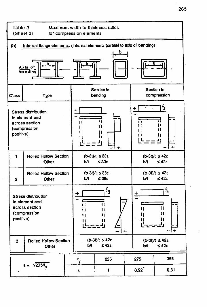
265

Table 3 Maximum width-to-thIckness ratios

(Sheet 2) for compression elements

(b) internal flange elements: (Internal elements parallel to axis of bending)

b1 • 1" 'i

Axisoi ____

I

b . II1L P:bifi OH] V ____ bend In

I

Section In Section In

Class Type bending compression

F-771 + I I Stress distribution + In element and i

ii • a across section ii I I

II Il II $ 1

(compression II II II

positive)

I Roiled Hollow Section (b-3t)/t S 33E (b-3t)/t :5 42

Other bit :533c bit :942c

Rolled Hollow Section (b-3t)/t :5 38E (b-3t)/t S 42

2 Other b/t :938c b/t S42z

± I I I I Stress distribution In element and

II across section

ii Ii Ii

(compression II II II II

positive)

— -J —4- —+

3 Rolled Hollow Section (b-31)It fb 42E (b-3t)It S 42E

Other b/t S 42 bit :942c

f, 235 — 275 355

e- 4235If £ 1 092 0.81

266 Table 3 Maximum width-to-ihiCkneSS ratios

(Sheet 3) for compression elements

(C) Outstand flanges:

j t C .r J

Rolled sections Welded sections

Class Type of Flange subject Flange subject to compress ion and bending

section to compression

Tip in compression Tip in tension

ac1 1ac, Stress distribution In element

_____________

I 1+ ________

j+ ________

+ .1 (compression positive)

II Pr! c j __ c

I, t I

IN lOt 1 Rolled c/t:5 lOt c/I ~5 - cit 15

CL a4

9e 9e Welded c/t9c c/t5 - c/I 15

a a4

lit lit Rolled c/tS lie cit S - cit 15

2 a

-

—4a

The lOt Welded cftS lOt c/I I -

a c/I ~

a'1

Stress distribution In element I I + ---1 +

(compression positive)

- C oil-

II

Rolled c/t -5 15c c/I S 23E '4 CT

Welded c/IS 14E c/t S 21e '

For ka soo lablo 5.3.3

'1235/f y

ly 235 275 - 355

I C I

1 0 .92 0.81

267

Table 3 Maximum width-to-thickness ratios (Sheet 4) for compression elements

Moles: h

Refer also to (C) 1 T (Does not apply to •Outand flanges I I b angles in continuous (see Sheet 3). II contact with other

U ...L. components)

Class Section in compression

Stress distribution ± I I across section - (compression positive)

h b + h 3 —:915z : S23

Tubular sections:

0 Class Section In bending and/or compression

1 d/'t S50€ 2

2 d/t S70Z

3 d/t90c2

235 275 355

e. 4235If 0,92 0,81 £ 1

£2 1 0,85 0,66

Table 4 Selection of buckling curve for a cross -section

Cross section Umits Budding Budding about axis curve

Rolled I-sections hib , 1,2: t:540mm y-y a

z-z b

40mm ct 100mm -

b

hib :5 1.2:

j t~ 1OOmm

tf >lOOmm y - y z-z

ci d

Welded I-sections 40mm y

- y b

Tt ' 1{ YJFY t> 40mm

-

y_y z-z

C

d

Hollow sections hot rolled any a

0 0 [] cold formed - using any b

cold formed USlflQfyai any c

Welded box sections z

I generally (except as below) any

thick welds and

' L .

b Air <30 h/t<30

y-y z-z

C

C

U-, L-, T- and solid sections

any C

)See 5.5.1.4(4) and figure 5.5.2

- 0.5 section factor r,,

[]

time t qastemp. 10 20 30 50 100 150 200 250 1 300

[mm] °c]

0 20 20 20 20 20 20 20 20 20 20

15 739 95 1b4 226 3)) 514 612 664 691 705

30 842 215 367 484 637 781 814 824 829 831

45 902 343 552 682 308 877 888 893 895 896

60 945 467 700 814 897 930 936 939 940 941

75 979 580 809 390 949 967 972 974 975 976

90 1006 678 089 954 985 997 1000 1002 1003 1003

Table 5 Calculated temperature of non-insulated steel members as a

function of the section factor FN and time t (€ r=0 • 5 j

Lt=30 secs)

269

Appendix C: Swedish Institute of Steel Construction 270

Fire Engineering Design of Steel Structures [ Pettersson, 1976 ]

LOADBEARING Determine, 1mm i awe - u

STRUCTURE load which shall not cause the structure to

collapse under fire exposure conditions

rDetermine the design fire load frotn Table 1 2., -and calculate the opening factor In

apcordance with Fig. 2

Conversion of the fire load and opening fac-

tor for the fire comportment in question Into equivalent fire load and opening factor

In accordance with Table 8

[

if the lire load is low or if conditions are favourable in other respects, see 11

he structure can be constructed without insulation. If this cannot be done, the

he structure must be protected by insulation or a suspended ceiling

Uninsulated structure

Determine the resultant

emissivity from Table 4.

Calculatethe F5 /V 5 ratio

laccording to Fig. 3

Insulated structure

Choose auitahle insulation material. Assume the requi-

site thickness. Calculate the ratio

/ any of 'N f these ?nater'\

mis used: gypsum plaster

isl,s mineral wool

slabs

) sprayed mm--.cral wool

Determine the d1/1 value of the insulatio

material used from

Structure protected by suspended ceiling

Choose . P suitable suspended

ceiling - -

Determine the maximum tem-

perature of the suspended cell

log In the event of fire

the tem-

/ perature of suspended ceiling high

er than the critical sus-

pended ceiling temperaj

ture

No

Yes

Yes

No

Determine the maximum steel temperature from

I Determine the maximum steel

Determine the maximum

steel temperature from

the maximum steel

re fm Table 7 b

Is the load

from

No ble I greater Yes attt

crmined

han he crit-

ical load

Columns

Assess degree of expansion, If expan-

sion is restrained, from Fig. 4 -

Determine the critical load for

compression only, from Fig.5

simultaneous flexure and comp.es-sion, according to Section 10.3 in

Main Section the risk of out-of-plane instability,

according to Section 10.4 in Main

Section

Girders

the rate o

ne

alt. 1) lt. I) reduce Insulation]

I

alt. 1) Increase Insulatio

P

n

alt. 2) stop design ait.2) increase steel dimensions

lait.2) alt.3) give the construction a more favourahl

_______________ F./V. and A1/V.

Fig.1 Flow chart which illustrates the design procedure.

271 DETERMINATION OF THE DESIGN STATIC LOAD IN THE EVENT OF FIRE

Table I Static load which shall not cause a Loadbearing structure to collapse

under (ire exposure conditions

It shall be shown that 1 during a complete fire process, the structure will not collapse due to the most dangerous combination of

dead load snow load, multiplied by the load factor 1.2 Live load, multiplied by the load factor 1.4

Calculation: The dead load Is to be calculated in the conventional way For the snow load, the values to be applied for the static and mobile constituents are to be 80% of the values according to current building regulations V The following values are to be applied for the live load

Type of premises Static load kgf/m2 Iktl/m 2 1

Mobile load kgl/m 2 IkN/m 2 1

Buildings in which complete evacuation 21jcplc in the event of fire cannot j assumed with absolute certainty

Dwelling and hotel rooms, hospital wards, etc 35 10.351 70 10.701 Offices and schools(classrooms and group study rooms) 35 I 0.351 100 I 1.001 Shops, department stores, assembly halls (excl. records rooms and warehouses containing compact stacked loading) 35 10.351 250 12.501

flulldigs In wlilch complete evacuation oIpepIc in the event of It re cnn be assumed with absolute certainty_

Dwelling and hotel rooms, hospital wnr(is, etc 35 10.35 35 10.351 Offices and schools (classrooms and group study rooms) 35 10.351 55 10.551 Shops, department stores, assembly halls (cxci. records rooms and warehouses with compact stacked loading) 35 10.351 70 10.701

DETERMINATION OF THE DESIGN FIRE LOAD AND OPENING FACTOR 272

Table 2 Fire loads in various types of buildings and premises determined by means of statistical investigations. The values are referred to the total internal surface area of the lire compartments.

Type of building or premises

Fire load Fire load mean value standard deviation

Mcal/m 2 IM3/m 2 1 Mcal/m 2 IM3/in 2 l

Design fire load. Fire load denoting the 80% level Mcal/m 2 IMJ/m 2 1

1 Dwellings' 2 rooms + kitchen 35.8 1149.9 5.9 j 24.7 40.0 1167.5

3 rooms + kitchen 33.1 1138.6 I 4.8 1 20.1 I 35.5 1148.6

2 Office buildings bC Technical offices 29.7 1124.4 7.5 I 31.4 I 34.5 1144.5 I (architects officcs etc) Economic and ad- 24.3 1101.7 I 7.7 I 32.2 31.5 1131.9

ministrative offices (banks, insurance companies, etc) All the investigated 27.3 1114.3 I 9.4 I 39.4 I 33.0 1138.2 I offices taken together

3 S choolsb Junior level schools 20.1 I 84.2 I 3.4 I 14.2 23.5 I 98.4

Intermediate level 23.1 96.7 I 4.9 I 20.5 28.0 1117.2 I schools Senios level schools 14.6 I 61.1 I 4.4 18.4 17.01 71.2 I All the investigated 19.2 80.4 I 5.6 I 23.4 23.01 96.3 I schools taken together

4 Hospitals 27.6 1115.6 I 8.61 36.0 I 35.01 116. 5 I

5 Hotels 1) 16.0 I 67.0 I 4.61 19.3 I 19.51 81.6 I

The fire load due to floor coverings is not included in the values quoted.

h The values quoted apply only to the fire load due to furniture and fittings. Any addi-

tional fire load Is to be calculated according to Equation (3. 1 a) in the Main Section.

C According to Swedish regulations, an entire office apartment is defined as a fire com-partment. Since there were difficulties during the statistical investigation In determi-ning the sizes of the fire compartments, the quoted values of the fire load apply to each office room. Furthermore, it is to be noted that office buildings are often constructed In such a way that each office room can be designated as an individual fire compartment. In Subsection 3.2.2 In the Main Section, distribution curves are also given for the fire load with reference to the floor. area. These values can be used In determining the fire

load per n 2 of the total internal surface area when division into fire compartments is

arbitrary.

CONVERSION TO EQUIVALENT FIRE LOAD AND OPENING FACTOR 273

TabLe3 Factors for the conversion of the actual fire load and opening factor for different types of fire compartment ft to equivalent fire load and opening

(actor applicable to fire compartment Type A(standard fire compartment)

Equivalent fire load k 1 . actual fire load Equivalent opening factor k actual opening factor

Factor k f

- - Fire compartment

Actual opening factor (mh/2)

Type Description of enclosing 0.02 0.04 0.06 0.08 0.10 0.12 construction

A Thermal properties 1.0 1.0 1.0 1.0 1.0 1.0

corresponding to average values for concrete, brick and lightweight concrete (standard Fire compartment)

13 Concrete (l00%) 0.85 0.85 0.85 0.85 0.85 0.85

C Lightweight concrete (100%) 3.0 3.0 3.0 3.0 3.0 2.5

D 50% concrete 1.35 1.35 1.35 1.50 1.55 1.65

50 % lightweight concrete

E 50% lightweight concrete 1.65 50 35 1.50 1.75 2.00

33 % concrete

from the inside outwards, 13 mm gypsum plaster- ti1 s.j€t

17% board V1

100 mm mineral wool 8y)UIi- /LS[.

brickwork ______________

Fb •80 % uninsulated steel sheeting 1.0-(0 1.0-0.5 0.8-0.5 0.7-0.5 0.7-0. 5 0.7-0. 5

20 % concrete

G 20% concrete 1.50 1.45 1.35 1.25 1.15 1.05 41 43 4 f3f5

2xl3 mm gypsum plaster- board ________

LocttJ 80% 100 mm air gap . pts_{_r

2x13 mm gypsum plaster- Lboard

COL 940LD

Fateel sheeting 3.0 3.0 3.0 3.0 3.0 . 2.5

100 100 mm mineral wool steel sheeting

DETERMINATION OF THE MAXIMUM TEMPERATURE IN THE EVENT OF FIRE IN UNINSULATED STEEL STRUCTURES

274

Calculatio!! procedure:

Determine the resultant emissivity E

Determine the F 8/V9 ratio Determine the maximum temperature 0

max

Table 4 • Resultant emissivity c for different constructions. The values yield results on the safe side (Main Section, Subsection 5.2.4)

Resultant Type of construction emissivity cr

1 Column exposed to fire on all sides 0.7 2 Column outside facade 0.3 3 Floor girder with floor slab of concrete, only the underside of

the bottom flange being directly exposed to fire 0.5 4 Floor girder with floor slab on the top flange a

Girder of I section for which the width-depth ratio is not less than 0.5 0.5 Girder of I section for which the width-depth ratio Is less than 0.5 0.7 Box girder and lattice girder 0.7

a More accurate values of ( r which take into account the width-depth ratio b/h and spacing-depth ratio c/h of the girders are given In Fig. 5.2.4 b In the Main Section

i_ ~P_14 wp~ [~P~

A-A 1 + A 2 ...+A6 -b 1 h 1 +b2h2 +... +b6h6 opna

h_* FACTOR

A[ AX ATh A - 2 [L,L2+1113+L2L3] At

Fig. 2 Calculation of the opening factor for a fire compartment with vertical openings. L1, L2 and L3 denote the Internal dimensions of the fire compartment

—i Table 5 The ratio F 5/V (m ) for rolled I girders for two different cases of exposure

275 to radiation

Steel All surfaces of the One side of one section steel section cx- flange not exposed

posed to radiation to radiation

I I EA 100 275 227 120 277 229 140 260 215 160 240 199 180 232 192 200 217 180 220 200 166 240 183 152 260 175 146 280 169 140 300 157 130 320 145 121 340 138 115 360 132 ItO 400 123 104

IlEfl (xre) tOO 226 188 120 208 173 140 192 160 160 174 144 180 163 135 200 151 126 220 143 119 240 134 III 260 130 lOB 280 126 lOS 300 119 99 320 112 94 340 109 91 360 105 88 400 100 85

IP 80 440 380

100 400 346 120 369 321 140 343 299 160 317 277 180 298 260 200 277 242 220 260 227 240 242 212 270 231 203 300 220 193 330 205 180 360 190 167 400 178 157

i t

Column within a

h

F fire compartment v cross section area

d . 2h+ Iib-2d

r7mh B

hJ1'J

F 2h + 2b)

V cross section area) F_fl

F Column, immediately

2h + b outside a window

V cross section area opening S

Floor structure,com- --1-4-----F _______ posed of steel beams F - - = I

— with a co ncrete slab, supported on the lowert : .:• : j ""jl bt t

B

i flange of the beasts t L

• :.. ' Beams with a floor slab, supported on F 2h + 3b - 2d the upper flange of v cross section area the beams s

. •.bi

-I F s 2h+b - =

V cross section area B

Floor slab beams of ' • F 2b 1 + 2h 1 truss type (F 3 /v 9 S

_ ( lower flange) = cross section area

determined for each Lk__1 8 of lower flange part of the truss) 0 _____

F b2 + 2h2

,r J Lt h, j- (upper flange) = cross section area

b, j of upper flange 0

F

- JL (diagonal) =

19 d

Ok

Fig. 3 Examples of calculatingF 8 /V s (m 1),the ratio of the area per unit length exposed to fire (m 2/m) to the enclosed steel volume per unit Length(m 3/m) for different types of construction. See also Table 5 b(Maln Section, Subsection 5.2.5)

276

the cquIvncnt flic load q(Mcal/m 1 )I MJ/tn 2 l. C (lUlValCflt opening factor AVh/A t (n') nud the

F./V, ratio of the construction (m') For different resultant cnissivitIcs cr 277

A A F, 0max AVi F, °m$ic AV F, 0m. i A rh Fs q

•-;--- 7 S

q --

8

q 7 A 1 y , (, 1 , t, It C, 1, C , 1 (

0.3 0.5 0.7 0.3 0.5 0.7 03 0.6 0.7 ' 0.3 05 0?

- - -;; 325 35 370 no .100 420 ItO 25 390 425 41 155 190 i.flO

75 3G 33; 105 .- . 76 135 415 460 flO Ifl 41`10 490 50 510 525 530

100 305 410 425 •• 100 150 400 470 75 185 500 600 75 525 530 535

0.01 125 3*0 425 435 0.01 125 •n;o 470 475 OOt too 105 605 505 001 100 530 535 035

150 125 435 4•10 too iio 470 480 125 500 500 510 125 530 535 510

200 435 4.15 413 200 175 180 480 150 505 510 OtO 100 035 510 ilO

400 450 450 450 too 480 185 485 00 505 • StO 515 300 535 510 510

so - 34 F-4 i6" - 100 - GIG L $00 .10 tIO $0

75 '110 4-15 475 75 500 510 7)55 50 500 550 075 50 555 600 6.7.'

100 115 4sO 520 100 010 575 695 75 560 600 620 70 GtO 610 r..0

0.02 125 490 so 515 0.02 125 065 500 610 100 595 620 630 0.02 100 510 650 655

150 500 510 555 I5O 556 605 il I5 0,02 125 515 630 010 25 125 650 0 55 60

200 510 560 575 200 505 020 (125 150 525 010 0-15 1104 0.01 50 570 6$.. 700

*00 575 7745 5115 '100 625 530 530 20 200 635 11-IS 550 - -I s

50 285 3034. 60 jool rtu(eiJ .1 00 450 650 G50 2 355 15 G tO

75 350 400 450 76 490 5 50 soo 50 -105 sos 025 0,00 50 525 600 700

150 105 son Sin 0.01 too r.sn (1(0 655 0.01 is ss5 650 700 ,. .In. 010

50 4I)

090

.10 710 I...'.

0.01 i's ISO 5 I 555 15 $25 ron 4)55 695 lOS - 25

650 2853I0

700 710

11 F" 008 75 520 700 770

10 , 150

21)0

$9' 550

555

600

CS, 4.15 1631 -

$ 0 G33 rM0 710

.175 50 -iiø 505 600 I _L..

300 (.25 64.4) 1.1)5 75 -$5 Iso 5 7 o. on 75 510 610 700 25 210 400

.040

.160 31 5

590

0 05 :°° .°::

nso 630 100 GIs : o 675 755 0 $2 75 oo (110

Ion .90 I,..., 84)0

0. on 0o 355 410 .185 $541 575) 635 720 75 0,05

too

(8.. 5115

(.20 670

070

735' 1.2. C,, 1.70 -

150

115

.150

•150

IS , 510

'MO - 200 1)00

1140374342

7 121 430 71. 750

- 25 505

_flO 50 0 4(0 7 340 Its r, - i;-' i23O' - !"0 515 , ID

- 300 615 r.so i33 100 -150 015 6113 50 310 375 504) 75 5.5

$00 .10 . 4 :fl 560

.1,0 .)0

75 270 20 05

530 100 125 iS))

505

555

593

650

070

710

75

0,12 100 125 .1 in

180 500

(Ito

700 0.01 125 .560 .14:1

too 530 IOn Ion Ion 6.73 75 73 $25 530 620 771 1544 51,0 54,., .163

0.08 t 3)4) 1 0 tO 'iöii' i'o I 1)0 CS, - -

304) r

.11)0 565

, 570.70

70

$90 I$fl 510 7740 75 3 I 40 SI))) - 25 -$20 $60 .1140

100 -ISO 590 660 0.12

° no 49) iO 79)5 5 1 30 0,02

50 004)

75 650

VI0 670

(.1.0 670

355 1910 700 760 ill 150 Sin (175 75 510 515 520

020 1126) 100 01.0 67., 61..

- 170 200 2410 50 t50 000 650 755 - ISO

0,01 123

520

520

520

525 525 e 75

$00 120

2-10

260

310

350

.1(40 - 200

23

575

355

1740 385 itIl 150 525 525 525

0.01 . 7 21_19_ 6 00

0.il $25 260 3110 510 50 $38 -ISo -1 1; 7, 200 530 530 030 23 110 :1)0 .,M0

i5a 310 430 620 75 -164) .575 -1Sf) *00 530 530 530 0.05 50 59.. 05 1) 760

1110 380 550 7011 0.51 100 -174. .180 IllS - 50 530 573 4.05 - .! !

300 -ISO 620 1100 525

ISO iSO -IllS

-InS '11(0

-171)1 -(713

,, 70

•o_ 100 S'JO 615

620

635

635

650 0,08 -

7 75 1.1•077

- III) - -

365 3741 -505

• 75 -ItO 120 .130 100 -$85 $95 504) 125 630 6-I5 050 25 290

50 4(0 •.iO 5.0 o ol IsO 130 -I-IS -(50 100 11)0 500 54))) ISO CII 6.0 '•' 0,12

7 40 ro 170 I.? 110 1 I) 44;0 - - jj' jo - rocO CGS

$50 150 155 160 73 535 570 5715 50 525 500 6(10 - - *00 64L, 710 -

11)0 11 *60 .11)5 $00 565 6(40 0(3 ' 0,01 75 620 690 -15 0.12 2-. Il-'

4:0

650

- •s -$65 .170 .1711 - 125 osS 0(0 6:00 - I!!!. ..2.L!_TOO 460 l's6)

._ 25 2(0 27(1 3_-'

-553

3l .I74)

500 533

150

200

6*0

625

6.70

635

035

615

25

19 1) 50

320

-180 350 550 4)55 54) 360 410 520

75

too 500 510 560 -

-100 635 11. 15 615 0,04; 75 .565 1150 7-10 0,30 75 4-'O 5....

0 610

730 0.0.-, , 1, 73 G O 1017 11(0 655 725 795 150 533 65

I'o 0 470 ''*0 7 SI 400 , - j - - $2 495 73 720

200 570 7)90 600 0.01 500 600 660 703 0,08

75 610 630 725 90 2-12..

- -ISO 500 601 605 *25 650 700 7111 - *00 670 730 780 0,30

'I 531

.4 6.0

7-. 790

790

- 890

- - - 25531103711 25 215 25T'O

75 ItO .5115 510 50 39)) .553 r, -.0 50 360 -1t5 510 - -

tOO 185 050 ron 0.043 75 -190 555 055 75 51)5 510 65((

0.01 115 535 600 610 100 565 4)20 710 0.12 lou 510 42(5 7342

iso 570 625 6.15 l7,5 125 620 670 750 125 625 675 800

13,5 200 630 4.61 750 - I73.)

315 435 . 1 s - - -

650 7-10 -

- 0.08

75 110 530 600

70 365 525 -17)3 100 000 605 670

-125 480 Silo $25 560 600 710

0. or 520 $80 525 010 150 615 705 765

150 520 560 650 25 160 250 271

100 r,s0 615 705 50 275 330 450

300 670 710770 75 350 130 5-50

- 50 250315 360 - 0.12 :0'

125 50.5 650

75 325 *00 455 25 475 575 715

0.08 $00 385 470 535 150 525 6-15 715

525 -535 530 000 200 600 725 - too -045 sqr, (ISO - - - 100 500 660 730

:too 4355 770 - 00 200 250 3:10

75 210 320 .110

0.12 2110 400 5$0

125 310 450 620

550 3110 510 690

200 500 600 760

300 1300 720 -

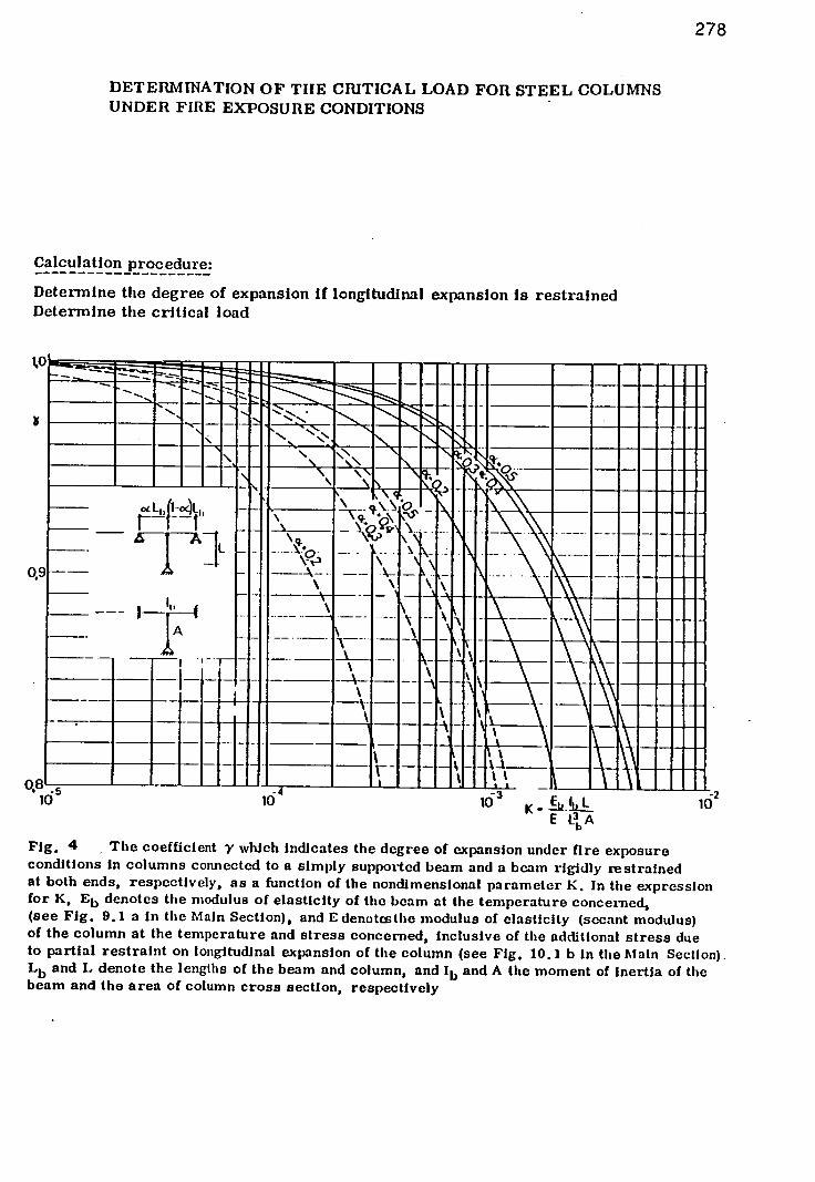
278

DETERMINATION OF THE CRITICAL LOAD FOR STEEL COLUMNS UNDER FIRE EXPOSURE CONDITIONS

Calculation procedure:

Determine the degree of expansion If longitudinal expansion Is restrained Determine the critical load

"Hi 11 mill

____• mill

I •iii

.

I uHI I' 111111111

itliflIll IHI, •111loll lI Jio • 1 11111 ___ I1I -2 10 10

EA

Fig. 4 The coefficient v which indicates the degree of expansion under fire exposure conditions in columns connected to a simply supported beam and a beam rigidly restrained at both ends, respectively, as a function of the nondimensional parameter K. In the expression for K, Eb denotes the modulus of elasticity of the beam at the temperature concerned, (see Fig. 9.1 a In the Main Section), and E denotes the modulus of elasticity (secant modulus) of the column at the temperature and stress concerned, Inclusive of the additional stress due to partial restraint on longitudinal expansion of the column (see Fig. 10.1 b In the Main Section). Lb and L denote the lengths of the beam and column, and lb and A the moment of inertia of the beam and the area of column cross section, respectively

1,0 1

O•8L 10

279 Fig. 5 Critical buckling stress CYk asa function of the steel temperature 8 and slenderness ratioX for a column under fire exposure conditions, made of structural steel with a nominal yield stress at room temperature of a s = 2200 (220), 2600 (260) and 3200 kgl/cm 2 1320 MPaI. y= coefficient indicating degree of expansion. When v I 1, the cross sectional factor l/d Influences the shape of the curves, but this Influence Is comparatively limited. The curves given have therefore been generally determined for i/d = 0.6, which fornormnal types of section results In design on the safe side. For determination of the critical load in a structure subject to simultaneous flexure and compression, see Section 10.3 In the Main Section. For determination of the critical load In a structure where there Is a risk of out-of-plane buck-ling, see Section 10.4 In the Main Section

I. 0I I I

, I

I

'I

I.

S I II

SI

S

i1II1IIIII4.. I.

I

IS

I S I S

II,

S

I

S

• I.

X A

HIHIHI I!! JI!IiiIifl

.

I.-

•

r,,4,HiiiL44.. iH I 4 ' I

I ..

IIHIiIiiiIIh 0 50 100 150 200

X

HHIH1III11III IL!

Ipi fl I

I ILIIL. hini A

kg1.kni

IMP-4 200( 1200,

150( (i5c

0c

50( {5

kgfin

MP

200C t20c

150C 050

BE

SOC (501

10 Zs.]

281

o sgf/cn?

2000 t200j

1500 (150)

1E1i I ±

M 2 aL 2200kgf/c - 220 (ivipa) %75

I T- '1200'

300

0 50 F i ± po

55 oi- - ..' ....

600

'I p_nj

a. kg1/c — - - -

IMP N

2000 - --- - --- — -i--- (20 -..- - .- -. .- oó k gf/cii 2 -

cr. 220 -IMPal 1-05

1500 ---- --- 1150)

100 Ioo - "/f3001 I

.-'.l

— ; r -i - - i-- - - -

1Ttt± 0 50 100 150 200

1

Appendix D: Fire Protection Insulation 282

[ASFPCM, '88]

VULTEX

I. Product description Sprayed Vermiculite

ManuFacturer I Iawk Business Services Limited Tel: 0635 524272

Fire Protection & Insulation Division, Telex: 848507 I IJULPI I 0

Kings I louse, Kings Road, Newbury, Fax: 0635 35053

l3erks, RGI4 5RA.

Availability From approved applicators. Contact manufacturer.

Protection technique Profile, box and solid.

Application technique Factory prepared mix, mixed with water on site then spray or hand applied.

Steel preparation Steel must be degreased and wire-brushed to remove loose scale.

requirements if steel is primed advice should be sought from the manufacturer.

Additional tnccl,nnlcal None up to 65mm and 4 hour's fire resistance for 3 and 4 sided application.

fixing Mesh or equivalent may be needed in other cases.

Nominal density 715 kg/n' npplicd.

Thickness Range it) - 80mm

Fire resistance range

a) Up to 4 hours. h) lip/A 26-310.

II. Constraints ror a) Minimum thickness 10mm.

fire resistance U) Maximum thickness unrcinforced 65mm.

Appearance Light pink textured surface.

On site use

For interior, semi-exposed (cg not subject to direct weather) exposed during construction period but may be required to be overcoa(ed with Vultex Weather

Shield.

Durability Resistant to frost, vermin and mould growth and limited attack by water.

IS. PerFormance In oilier Non combustible in accordance with BS 476: Part 4, so complies with class 0

BS fire tests as defined in the Building Regulations, 1985.

16. Other nppllcntioiis a) Thermal insulation U) Sound insulation

Fire protection of ductwork Fire protection of concrete

c) General fire protection - internal linings to external walls, cavity barriers etc.

II,,/A

up to

Dry thickness in mm to provide Fire resistance or

½ hour I hour I ½ Iour 2 hour 3 hour 4 hour

30 10 10 14 18 26 35

50 10 12 17 22 33 43

70 10 13 19 25 37 48

90 10 14 21 27 39 52

110 10 15 22 28 41 54

130 10 16 22 29 42 56

150 It) 16 23 3() 44 57

170 tO 16 23 30 44 59

190 10 16 24 31 45 59

210 10 17 24 31 46 60

230 10 17 24 32 46 61

250 10 17 24 32 47 61

270 10 17 25 32 47 62

290 10 17 25 32 47 - 62

310 tO 17 25 32 48_ 63

Linear interpolation is permissible he I ween values of ii p/A

283

41 0.1

horde

Box

Solid

1• P,ofile

Box

Solid

284

References * Not used

Almand, K. H., Thomas, l.A., Bennetts, I.D., Proe, D.J., Lenins,

R.R.(08/1989), Fire in offices, BHP , MELB. RES. LAB., Rep. No.

MRL/PS69/89/005.

Anderberg, V. (1986), Modelling steel behaviour, Lund Institute of

Technology, Lund, Sweden.

Anderberg, Y. (1983), RILEM Committee 44-PHT, Behaviour of steel

structures at high temperatures.

Anderberg, V. (1976), Fire exposed hyperstatic concrete structures, An

experimental and theoritical study, Lund Institute of Technology, Lund,

Sweden.

Anderberg, V. , Forsen, N.E., Aasen, B. (1985), Measured and predicted

behaviour of steel beams and columns in fire, Fire safety Science

Proceedings of First International Symposium.

Arbed Recherches (1986), C.E.C. Agreement Number No 721 0-SA / 502,

Computer assisted analysis of the fire resistance of steel and composite

concrete-steel structures (REFAO-CAFIR), Draft of final report 14.03.1986.

* Arbed Researches (1985), C.E.C. Agreement Number No. 7210- SA

/502, Computer assisted analysis of the fire resistance of steel and

composite concrete-steel structures (REFAO-CAFIR), Final report, Period

01 .07.1982 - 30.06.1985, Appendix A.

285

* Arbed Researches (1958), C.E.C. Agreement Number No. 7210- SA /

502, Computer assisted analysis of the fire resistance of steel and composite

concrete-steel structures (REFAO-CAFIR), Final report, Period 01 .07.1982 -

30.06.1985, Appendix B.

Association of Structural Fire Protection Contractors and

Manufacturers Limited (ASFPCM) (1988), Fire Test Group (FTSG),

Steel Construction Institute (SCI), Fire protection for structural steel in

buildings, 2nd edition.

Barnett, J. R. (1985), Uses and limitations of computer models in structural

fire, Protection Engineering applications, Fire Safety Journal, Vol. 9.

Barnett, C.R. (1986), The behaviour of fire-exposed steel members before

and after failure, Vol. Ill, Pacific Structural Steel Conference, Auckland.

Beer, F. P. , Russell, E., Johnston, Jr. (1979), Mechanics of materials,

Mc Graw-Hill.

Bernstein, M.L., Zaimovsky, V.A. (1979), Mechanical properties of metals,

Mir Publishers Moscow.

Beton Kalender (1983), Wihelm Ernst & Sohn, Berlin! Munchen.

*BIId, S., Trahair, N.S. (1988). Steel Colunm Strength Models. J. Construct.

Steel Research, Vol. 11.

Braimi,P., Tsitouri, V. (1987). Fire Protection of Building Structures.

National Technical University of Athens, Athens, Greece.

S. .

British Research Establishment Digest 317 (12/1986), Fire Resistant

Steel Structures: free standing blockwork-filied columns and stanchions,

British Steel Corporation, Fire Research Station, BRE Publication.

BRE News of Fire Research (01/1987), Fire Resistant of Steel

Structures, Fire Research Station, BRE Publication.

British Research Establishment (1988), Thermal bowing and how it

affects building design, BRE Information, Paper IP:Part 21, BRE.

British Standards Institution (1969), Specification for the use of

structural steel in building, Part 2: Metric Units.

British Standards Institution (1972), BS 476: Part 8: Test methods and

criteria for the fire resistance of elements of building construction, BSI,

London.

British Standards Institution (1984), BS 6399: Part 1: Code of practice

for dead and imposed loads, BSI, London.

British Standards Institution (1985), Structural use of steelwork in

building, British Standard BS 5950: Part 1:1985, Code of practice for

design in simple and continuous construction, BSI, London.

British Standards Institution (1987),

Part 20: Methods for determination of the fire resistance of elements of

construction (general principles).

Kiffi

Part 21: Methods for determination of the fire resistance of load-bearing

elements of construction.

Part 22: Methods for determination of the fire resistance of non-loadbearing

elements of construction.

Part 23: Methods for determination of the contribution of components to the

fire resistance of a structure.

British Standards Institution (1990), Structural use of steelwork in

building, British Standard BS 5950: Part 8:1990, Code of practice for fire

resistant design, BSI, London.

British Steel; General Steels (1988), Manual that contains product

information relating to the hot-rolled structural sections produced to BS4:

Part 1:1980 and BS 4848: Part 4:1972 by British Steel plc., Reference No.

GS SOOl 14.10.88.

Brockenbrough, R.L.(1970), Theoretical stresses and strains from heat

curving, Proceedings of ASCE. J. Structural Division.

Bryl, S. (1985), Examples of calculations of fire resistance of the steel

members according to the European Recommendations of ECCS TC3,

Proceedings of the International Conference held in Luxembourg, Fire-safe

steel construction: practical design, 11-12 April 1984, Publication of the

Comission of the European Communities.

Butcher, E.G.,Chitty, T.B., Ashton L.A. (1966), The temperature attained by

steel in building fires, Fire Research Technical Paper NO.15, London,

HMSO.

NM

CIB W14 Workshop (1983), Structural Fire Safety, Fire Safety Journal,

Volume 6, No. 1.

Cooke, G.M.E. (1988), An introduction to the mechanical properties of

structural steel at elevated temperatures, Fire Safety Journal, Vol. 13.

Cooke, G.M.E. (1987), The structural response of steel I-section members

subjected to elevated temperature gradients across the section,PhD Thesis,

The City University, London.

* Culver, C.G. (08/1972), Steel Column Failure under Thermal Gradients,

Proceedings of ASCE, J. Structural Division.

Culver, C., Aggarwal, V., Ossenbruggen, P. (04/1973), Buckling of Steel

Columns at Elevated Temperatures, Proceedings of ASCE, J. Structural

Division.

Drysdale, D. (1985), An introduction to fire dynamics, A Wiley -

lnterscience publication.

ECCS (1983) - Technical Committee 3 - Fire safety of Steel Structures,

European Recommendations for the fire safety of steel structures,

Calculation of the fire resistance of load bearing elements and structural

assemblies exposed to the standard fire, Elsevier Scientific Publishing

Company, Netherlands.

Eurocode No. 4 (April 1990), Design of composite structures, Part 10:

Structural fire design, Draft.

289

Eurocode No. 3, Design of steel structures, Part 10: Structural fire design,

Draft April 1990.

Franseen, J.-M. (1987), Etude du comportement au feu des structures

mixtes acier-beton, Faculte des sciences appliquees,Universite de Liege,

Liege.

* Goh, C.C., Bennetts, l.D.,Foo,S.K., Thomas, I.R. (October 1989), Stability

and Strength of Steel Columns in Fire, BHP, Melb. Res. Labs., Report No.

MRL/PS65/89/003,.

Holman, J.P. (1986), Heat transfer, McGraw Hill, Inc.

Home, M.R. (1955), The stanchion problem in Frame Structures designed

according to Ultimate Carrying Capacity, Proceedings of ASCE, J. Structural

Division, Structural Paper 46.

Janss, J., Minne, R. (1981/82), Buckling of steel columns in fire conditions,

Fire Safety Journal,Vol. 4.

Kirby, B.R., Preston, R.R. (1988), High temperature properties of hot-rolled

structural steels for use in Fire Engineering design studies, Fire Safety

Journal, Vol. 13.

Kirby, B.R., Lapwood, D.G., Thomson, G. (1986), The Reinstatement of Fire

Damaged Steel and Iron framed Structures, British Steel Corporation,

Swinden Laboratories.

290

Klingsch,W.(1981/1982), Fire Resistance of Solid Steel Columns, Fire

Safety Journal, Vol.4.

Kounadis, A.N.(1987), Metal structures; Design and behaviour, Volume II

National Technical University of Athens Publication, Athens.

Kruppa,J. (1985), Presentation of the European recommendations for the

fire safety of steel structures, Proceedings of the International Conference

held in Luxembourg, Fire -safe steel construction: Practical design, 11-12

April 1984, Publication of the Commission of the European Communities.

Law, M.(1984),Steel structures, Proceedings of a European Symposium

held in Luxembourg, Fires in buildings,edited by Mourareau, A., Thomas, M.,

18 - 21 September 1984.

Lawson, R.M.,Newman, G.M. (1990), Fire resistant design of steel

structures - A handbook to BS 5950: Part 8, The Steel Construction Institute.

Lie, T.T. (03/1972), A numerical procedure to calculate the temperature of

protected steel columns exposed to fire, Fire Study No. 28, Division of

Building Research, National Research Council of Canada, Ottawa.

Lie, T.T.(1972), Fires and Buildings, Applied Science Publishers Ltd.,

London.

Lie, T.T.(1978), Fire resistance of structural steel, Engineering Journal,

American Institute of Steel Construction, Fourth Quarter, Vol. 15, No. 4.

291

Maihotra, H.L.(1982), Design of fire-resisting structures, Published by

Surrey University Press, London, U.K.

Maihotra, H.L. (March/April 1990), Introduction to Fire Engineering,

Building Control Fire Engineering.

* Marchant, E.W. (1972), A complete guide to Fire and Buildings, Medical

and Technical Publishing Co. Ltd.,England, U.K.

Milke, J., Analytical Methods for deetrmining fire resistance of steel

members, Section 3, Chapter 6.

Ossenbruggen, P.J., Aggarwal, V., Culver, C.G. (04/1973), Steel Column

Failure Under Thermal Gradients, Proceedings of ASCE, J. Structural

Division.

Pettersson, 0., Magnusson, S.-E., Thor, J. (1976), Fire Engineering

design of steel structures, Swedish Institute of steel construction, Publication

50.

Robinson, J.T., Latham D.J. (1986), Fire resistant steel design - the future

challenge, Proceedings of the International Conference on Design of

Structures against Fire held at aston University , Birmingham, U.K. on 15th,

16th of April, Edited by: Anchor,R.D., Malhotra, H.L., Purkiss, J.A. , Elsevier

applied science publishers.

Shield, T.J., Silcock, G.W.H. (1987), Buildings and Fire, Longman

Scientific and Technical, Longman Group U.K. Ltd.

292.

Smith, C.I. (March / April 1990), Fire Engineering and passive fire

protection, Building Control Fire Engineering.

Smith, C.I. (February 1983), Analytical methods aid the design of steel

framed buildings, Proceedings of the International Seminar, Three decades

of structural fire safety held at the Fire Research Station, BRE.

Sterner, E., Wickstrom, U. (1990), TASEF-Temperature Analysis of

Structures exposed to fire, User's Manuel, Swedish National Testing

Institute SP Report 1990:05, Fire Technology.

Terro,M. (1987), Computer Predictions of Fire Endurance in Structural

Elements, MSc, Dep. of Civil and Structural Engineering, University of

Manchester..

Thor, J. (1973), Deformations and critical loads of steel beams under fire

exposure conditions, Document D16: 1973.

Twilt, L.(1988), Strength and deformation properties of steel at elevated

temperatures: Some practical implications, Fire Safety Journal, Vol. 13.

Wainman, D.E., Kirby B.R. (1988), Compendium of U.K. Standard Fire

Safety Data, Unprotected Structural steel - 1, Published by BSC Swinden

Laboratories.

* Wickstrom, U. (1985), Application of the standard fire curve for expressing

natural fires for design purposes, Fire Safety: Science and Engineering,

ASTM STP 882 T.Z. Harmathy, Ed.,American Society for Testing and

Materials, Philadelphia.

293

Witteeveen, J., Twilt L.(1981/82), A critical view on the results of standard

fire resistance tests on steel columns, Fire Safety Journal, Vol. 4.

Witteveen, J., Twilt, L.(1972), On the behaviour of steel columns at

elevated temperatures, Colloquim on column strength, Paris 23rd and 24th

November 1972.

STEEL COLUMN BEHAVIOUR IN FIRE CONDITIONS

Documents

Transcript of STEEL COLUMN BEHAVIOUR IN FIRE CONDITIONS