STAVEBNÍ OBZOR - CKAIT

STAVEBNÍ OBZOR ČÍSLO 2/2018

Obsah čísla:

SEISMIC LIQUEFACTION ANALYSIS OF CAPITAL REGIONOF ANDHRA PRADESH STATE, INDIAG.V. Rama Subba Rao, B. Usha Sai

MONITORING DYNAMIC GLOBAL DEFLECTION OF A BRIDGE BY MONOCULAR DIGITALPHOTOGRAPHYGuojian Zhang, Guangli Guo, Chengxin Yu, Long Li

DOUBLE SIZE FULLJET FIELD RAINFALL SIMULATOR FOR COMPLEX INTERRILL AND RILL EROSIONSTUDIESPetr Kavka, Luděk Strouhal, Barbora Jáchymová, Josef Krása, Markéta Báčová, Tomáš Laburda,Tomáš Dostál, Jan Devátý, Miroslav Bauer

NONLINEAR FINITE ELEMENT ANALYSIS OF INSULATED FRP STRENGTHENED REINFORCEDCONCRETE COLUMNS SUBJECTED TO FIREOsama El-Mahdy, Gehan Hamdy, Mohamed Hisham

DISCRETE ELEMENT MODELING OF STRENGTH PROPERTIES AND FAILURE MODES OF QH-E LUNARSOIL SIMULANT AT LOW CONFINING STRESSESLi Yun-Li , Zou Wei-Lie1, Wu Wen-Ping, Chen Lun

TWO SIMPLIFIED MODELS OF COLUMN WEB PANEL IN SHEARMarta Kuříková, František Wald, Kamila Cábová

IMPACT OF CREEP ON FLANGE CLAMPING FORCEJan Plášek, Tomáš Ridoško, Jan Ekr, Jiří Kytýr, Roman Gratza

PERIODICALLY REPEATING SOUND AS A DISRUPTIVE AGENT IN BUILDINGSJaroslav Hejl

NUMERICAL SIMULATION OF STRESS WAVE PROPAGATION IN SAP CONCRETEZhenqun Sang, Zhiping Deng, Jianglin Xi, Huibin Yao, Jiang Wu

Article no. 13

THE CIVIL ENGINEERING JOURNAL 2-2018

-----------------------------------------------------------------------------------------------------------------

DOI 10.14311/CEJ.2018.02.0013 155

SEISMIC LIQUEFACTION ANALYSIS OF CAPITAL REGION

OF ANDHRA PRADESH STATE, INDIA

G.V. Rama Subba Rao1 and B. Usha Sai 2

1. Department of Civil Engineering, Velagapudi Ramakrishna Siddhartha Engineering College, Vijayawada, Andhra Pradesh, India; [email protected] 2. Department of Civil Engineering, Velagapudi Ramakrishna Siddhartha Engineering College, Vijayawada, Andhra Pradesh, India; [email protected]

ABSTRACT

Liquefaction is a phenomenon happens in a loose, fully saturated cohesionless soil in undrained condition subjected to cyclic loading. During liquefaction of the soil lost its shear strength when the mean effective stress is made equal to zero due to the progressively increasing excess pore water pressure. Liquefaction may cause failure of foundations, resulting in collapse of structure, even if the structure is designed as an earthquake-resistant. Liquefaction depends on characteristics of subsurface soil. Amaravathi is a new capital of Andhra Pradesh State, India. The construction activities in the capital region are swiftly increasing. It is essential that the new structures constructing in capital should be assessed for liquefaction susceptibility. In the present investigation an attempt has been made to assess the liquefaction susceptibility of various sites in the capital of Andhra Pradesh State, India. The liquefaction analysis is carried out by using simplified method which mainly relies on Standard Penetration Test (SPT) value.

KEYWORDS

Liquefaction, SPT, Susceptibility, Magnitude of Earthquake

INTRODUCTION

Earthquakes are most powerful natural disasters which are unavoidable. The hazards associated to earthquakes are referred to as seismic hazards. During an earthquake there is release of energy which reaches to the ground surface and to the structures by means of seismic waves. One of the major causes of destruction during an earthquake is the loss of strength & stiffness of cohesionless soils. This phenomenon called liquefaction occurs mainly in loose & saturated sand. When an earthquake shakes loose saturated sand, the grain structure of soil tends to consolidate into more compact packing. The soil liquefaction depends on the magnitude of earthquake, intensity & duration of ground motion, the distance from the source of the earthquake, site specific conditions, ground acceleration, type of soil and thickness of the soil deposit, relative density, grain size distribution, fines content, plasticity of fines, degree of saturation, confining pressure, permeability characteristics of soil layer, position & fluctuations of the ground water table [1, 2]. The purpose of the study is to evaluate the liquefaction susceptibility of various locations in the capital of Andhra Pradesh state, India using penetration resistance value from standard penetration test after necessary corrections. Firstly Cyclic Shear Stress Ratio (CSR) that would be induced due to earthquake was computed. In calculating CSR, the peak horizontal ground

mailto:[email protected]


Article no. 13


-----------------------------------------------------------------------------------------------------------------

DOI 10.14311/CEJ.2018.02.0013 156

acceleration value (amax) was selected based on region as mentioned in [3]. Seismic zoning map of India prepared based on the peak ground acceleration (PGA) induced by the maximum considered earthquake. Secondly determine the Cyclic Resistance Ratio (CRR) using the corrected penetration resistance value. Finally factor of safety against liquefaction (FOS) susceptibility is also determined which is the ratio of CRR to CSR. Variation of factor of safety versus depth for various magnitudes of earthquake is also studied.

REVIEW OF LITERATURE

There are two general approaches for the assessment of liquefaction. One is the laboratory testing of undisturbed samples and other is the use of empirical relationships developed mainly based on field tests [4]. The later approach is the dominant approach and is common in practice. The main reason for the selection of later approach is due to the experimental difficulties and high cost in the former approach. In India, most widely used in-situ test carried as a part of sub-soil exploration is SPT. Liquefaction susceptibility assessment using SPT value is the most common empirical method. [5, 6, 7] have evolved a method for liquefaction susceptibility using SPT based on both laboratory and field based data. Liquefaction susceptibility analysis of Kathmandu valley was carried by [8]. Liquefaction potential prediction of Coimbatore city was done by [9]. A liquefaction analysis of alluvial soil deposit for Kolkata city has been carried by [10, 11].

STUDY AREA

Amaravathi is the new capital of Andhra Pradesh State, India. Map of Andhra Pradesh with Capital Region Development Authority (CRDA) region is presented in Figure 1 [12]. Seed capital has land area about 121.4 square kilometres. The seed capital development area will comprise the Andhra Pradesh State Legislative Assembly, Legislative Council, High Court, Secretariat, Raj Bhavan, quarters for the ministers and officials, and the township for government officials.

Fig. 1. - Andhra Pradesh Map with CRDA Region

Article no. 13


-----------------------------------------------------------------------------------------------------------------

DOI 10.14311/CEJ.2018.02.0013 157

LIQUEFACTION SUSCEPTIBILITY ANALYSIS

The liquefaction susceptibility analysis was carried out using simplified method proposed by [5, 6, 7]. In the beginning in the simplified procedure, the CSR that would be induced due to earthquake was computed. Subsequently using SPT, the CRR of in-situ soil was determined. Further, factor of safety against liquefaction was computed which is the ratio of CRR to CSR.

The CYCLIC SHEAR STRESS RATIO (CSR) is calculated from the following equation:

𝑪𝑺𝑺 = 𝟎. 𝟔𝟓 (𝒂𝒎𝒂𝒙

𝒈(

𝝈𝒗𝟎

𝝈𝒗𝟎′ ) × 𝒓𝒅) (𝟏)

Where, amaxis the Peak ground acceleration

g is the acceleration due to gravity

= z is the Zone factor

Seismic zoning map of India prepared based on the peak ground acceleration (PGA) induced by the maximum considered earthquake [3].

𝜎𝑣0is the total overburden pressure (in kPa)

𝜎𝑣0′ is the effective overburden pressure at the same depth (in kPa)

rd is the stress reduction Coefficient

𝑟𝑑 = 𝑒[𝛼(𝑧)+(𝛽(𝑧)×𝑀)] (2)

M is magnitude of the earthquake

𝛼(𝑧)=−1.012 − 1.126 𝑠𝑖𝑛 [𝑧

11.73+ 5.133] (3)

𝛽(𝑧)=0.106 + 0.118 𝑠𝑖𝑛 [𝑧

11.28+ 5.142] (4)

In the above two equations Z is the depth of the soil stratum

The CYCLIC SHEAR RESISTANCE RATIO (CRR) is calculated from the following equation:

𝐶𝑅𝑅 = 𝑒[

(𝑁1)60𝑐𝑠14.1

+[(𝑁1)60𝑐𝑠

126]

2+[

(𝑁1)60𝑐𝑠23.6

]3

+[(𝑁1)60𝑐𝑠

25.4]

4−2.8]

(5)

Where (N1)60CS is the corrected SPT value including correction for fines

Factor of Safety against Liquefaction (FOS) is ratio of CYCLIC SHEAR RESISTANCE RATIO

(CRR) to CYCLIC SHEAR STRESS RATIO (CSR).

FOS = 𝐶𝑅𝑅

(𝐶𝑆𝑆𝑀𝑆𝐹⁄ )

(6)

Where CRR is the Cyclic Shear Resistance Ratio

CSR is the Cyclic Shear Stress Ratio

MSF is the Magnitude Scaling Factor

Article no. 13


-----------------------------------------------------------------------------------------------------------------

DOI 10.14311/CEJ.2018.02.0013 158

𝑀𝑆𝐹=102.24

𝑀2.56 (7)

In which M is the Magnitude of the Earthquake

If the value of Factor of Safety against Liquefaction is less than or equal to 1, the soil is susceptible to liquefaction (L). If the value of Factor of Safety against Liquefaction is greater than 1, the soil is not susceptible to liquefaction (NL). Standard Penetration Test (SPT) was conducted as per the guidelines of [13]. The SPT is carried out in drilled boreholes, by driving a standard 'split spoon' sampler using repeated blows with a 63.5kg hammer falling through 750mm. The bore holes have been drilled using rotary hydraulic drilling of 150mm diameter up to the rock depth. The hammer is dropped on the rod head at the top of the borehole, and the rod head is connected to the split spoon by rods. The split spoon is lowered to the bottom of the hole, and is then driven for a depth of 450mm, and the blows are counted normally for each 150mm of penetration. The penetration resistance (N) is the number of blows required to drive the split spoon for the last 300mm of penetration. The penetration resistance during the first 150 mm of penetration is ignored. The 'N' values measured in the field using SPT procedure have been corrected for various corrections recommenced for evaluating the seismic borehole characteristics of soil.

First, corrected 'N' value i.e., (N1)60 are obtained using the following equation:

(𝑁1)60 = 𝐶𝑁𝐶𝐸𝑅𝐶𝐵𝐶𝑅𝐶𝑆 𝑁 (8)

Where

CN is the Correction for Overburden Effect

CER is the Correction for Hammer Effect

CB is the Correction for Borehole Effect

CR is the Correction for Rod Length

CS is the Correction for Sampler

Then corrected 'N' values (N) is further corrected for fines content based on the revised boundary curves derived by [14] as described below:

The N value for soil shall be corrected for overburden is extracted from [11].

CN = 0.77 log10 [2000

σ0' ] (9)

Where is the effective overburden pressure.

Correction for Hammer Effect [CER] can be taken as follows:

For Doughnut hammer : 0.5 to 1.0

Article no. 13


-----------------------------------------------------------------------------------------------------------------

DOI 10.14311/CEJ.2018.02.0013 159

For Safety hammer : 0.7 to 1.2

Automatic Doughnut hammer : 0.8 to 1.3

Correction for Borehole Effect [CB] can be taken as follows:

CB = 1.00 for diameter of the bore hole = 65mm to 115mm

CB = 1.05 for diameter of the bore hole = 150mm

CB = 1.15 for diameter of the bore hole = 200mm

Correction for Rod Length [CR] can be taken as follows:

CR = 0.75 for l < 3m

CR = 0.8 for l = 3m to 3.99m

CR = 0.85 for l = 4m to 5.99m

CR = 0.95 for l = 6m to 9.99m

CR = 1.00 for l = 10m to 30m

Correction for Sampler [CS] can be taken as follows:

CS = 1.00 for Standard sampler

Correction for Fines Δ (N1)60 can be taken as follows:

Liquefaction, in the past, was primarily associated with medium to fine grained saturated cohesion less soils and soils with fines were considered non-liquefiable. [13] studied the liquefaction behaviour of silts and silt clay mixers over a range of plasticity values of interest by conducting cyclic tri axial tests on undisturbed as well as reconstituted samples and their behaviour was compared with that of sand. Saturated silts with plastic fines were found to behave differently from sands both with respect to rate of development of pore water pressure and axial deformations. Later on it was found by several investigators that certain soils with fines may be susceptible to liquefaction.

Δ(N1)60 = e[1.63+(

9.7

fc+0.001)-(

15.7

fc+0.001)

2] (10)

Where is the fines content

Corrected SPT value including correction for fines [(N1)60CS] is given by

(N1)60CS = (N1)60 + Δ(N1)60 (11)

Authors attended SPT conducting at Mandadam site (shown in Figure 2). The fines content present in soils was measured. Vulnerability of liquefaction evaluation in light of experimental

Article no. 13


-----------------------------------------------------------------------------------------------------------------

DOI 10.14311/CEJ.2018.02.0013 160

approach with SPT value (N value) was done at 107 locations those covers all the area of capital region of Andhra Pradesh.

Fig. 2. - Lifting of drop hammer for applying blows

DISCUSSION ON TEST RESULTS

Liquefaction susceptibility analysis was carried out using simplified method as proposed by [2, 3] based on SPT value. In the simplified procedure the Cyclic Shear Stress Ratio (CSR) that would be induced due to earthquake was computed. In calculating CSR, the peak horizontal ground acceleration value (amax) was chosen as 0.16g as mentioned in [4] for capital region of Indian State Andhra Pradesh. Subsequently using SPT, the Cyclic Shear Resistance Ratio (CRR) of in-situ soil was determined. Factor of safety against liquefaction is the ratio of CRR to CSR. Further, factor of safety against liquefaction for different magnitudes of earthquake (=4, 5, 6, 7, 7.5) was computed. Since the River Krishna is flowing through the capital region of Andhra Pradesh, throughout the analysis water table was assumed to be presented at ground level. A typical calculation of factor of safety against liquefaction for a magnitude of earthquake is presented in Table 1.

Article no. 13


-----------------------------------------------------------------------------------------------------------------

DOI 10.14311/CEJ.2018.02.0013 161

Tab. 1 - Liquefaction Analysis of Mandam Site for an Earthquake Magnitude 4

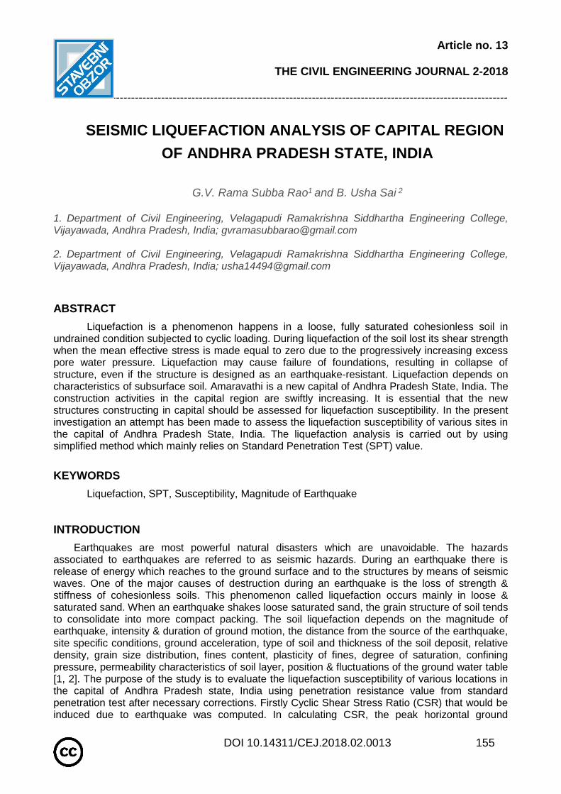
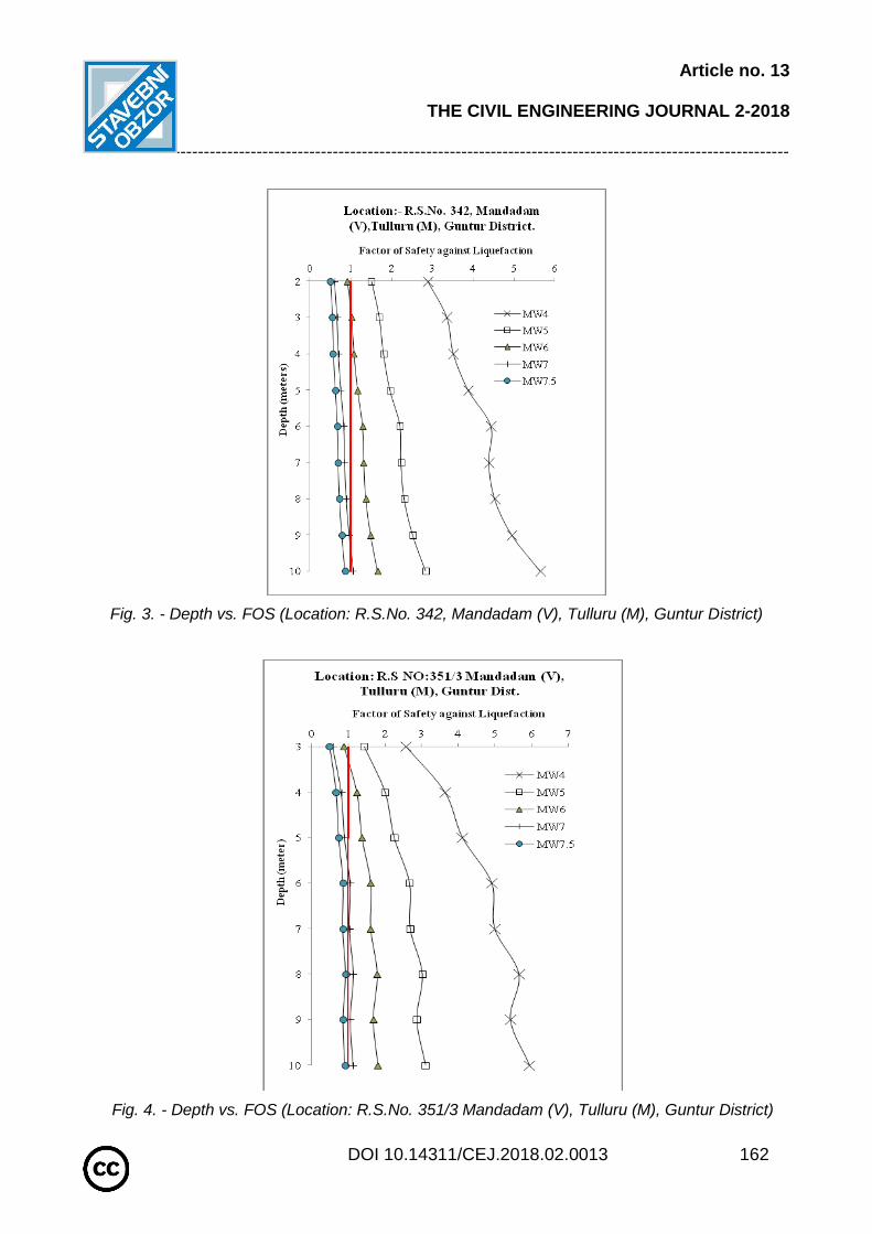
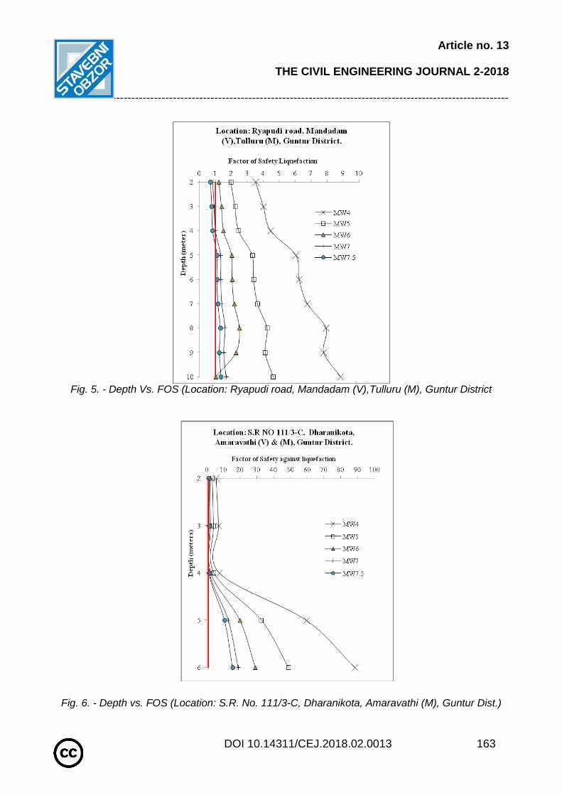
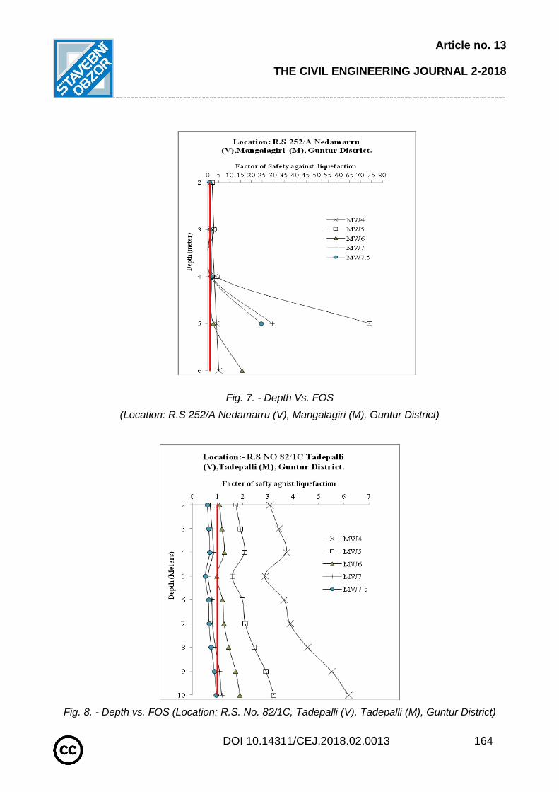
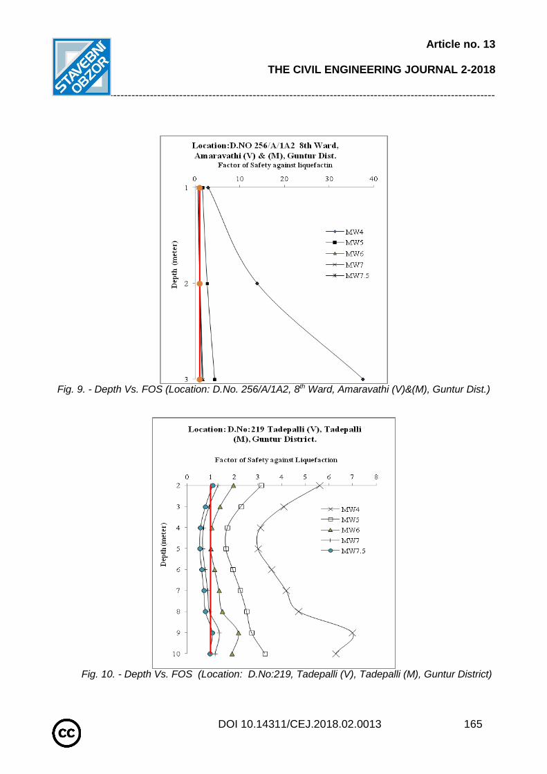
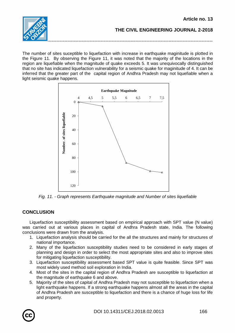
Liquefaction analysis has been conducted for other earth quake magnitudes also. Analysis carried in various locations of capital region of Andhra Pradesh State, India. Depth versus factor of safety against liquefaction for different Magnitudes of Earthquake at various locations of capital of Andhra Pradesh State is shown in Figures 3 to 10. It was observed from Figures 4 to 11, the Factor of Safety against Liquefaction is greater than 1 for Earthquake Magnitudes of 4 and 5 irrespective of depth for various locations. It was also noticed that when Magnitude of earthquake 6 and above, many of sites in the capital region of Andhra Pradesh State, India was prone to Liquefaction. At some locations (as depicted in Figure 7, 8 and 10) higher factor of safety against liquefaction was obtained due to presence of hard gravel (SPT value is more than 50) at lower depths.

Depth of Ground Water Table= AT GL

Peak Ground Horizontal Acceleration(amax/g)= 0.16

Depth,

Z

(m)

Depth,

Z

(m)

Observed SPT

Value

Saturated

Density (kN/m3)

Submerged Density (kN/m3)

Fines (%)

Corrected SPT [(N1)60]

(Eqn.8)

Correction for

fines(fc) [Δ(N1)60]

(Eqn. 10)

Corrected SPT

Value [(N1)60cs]

(Eqn.11)

Cyclic Shear Stress [CSS]

(Eqn.1)

Cyclic Shear

Resistance

[CRR7.5]

(Eqn.5)

Factor of

Safety (FS)

(Eqn.6)

Conclusio

n

2 3 2 19.68 9.87 97 1.64 5.49 7.14 0.19 0.10 2.57 NL

3 4 9 19.8 9.99 96 6.81 5.50 12.31 0.19 0.13 3.63 NL

4 5 12 20.08 10.27 94 8.26 5.50 13.77 0.18 0.15 4.11 NL

5 6 15 20.29 10.48 92 10.72 5.51 16.23 0.17 0.17 4.91 NL

6 7 15 20.6 10.79 98 10.08 5.49 15.57 0.16 0.16 4.99 NL

7 8 18 20.66 10.85 97 11.46 5.49 16.95 0.15 0.17 5.65 NL

8 9 16 20.74 10.93 97 9.71 5.49 15.21 0.15 0.16 5.42 NL

9 10 17 20.99 11.18 97 10.39 5.50 15.89 0.14 0.16 5.94 NL

Article no. 13


-----------------------------------------------------------------------------------------------------------------

DOI 10.14311/CEJ.2018.02.0013 162

Fig. 3. - Depth vs. FOS (Location: R.S.No. 342, Mandadam (V), Tulluru (M), Guntur District)

Fig. 4. - Depth vs. FOS (Location: R.S.No. 351/3 Mandadam (V), Tulluru (M), Guntur District)

Article no. 13


-----------------------------------------------------------------------------------------------------------------

DOI 10.14311/CEJ.2018.02.0013 163

Fig. 5. - Depth Vs. FOS (Location: Ryapudi road, Mandadam (V),Tulluru (M), Guntur District

Fig. 6. - Depth vs. FOS (Location: S.R. No. 111/3-C, Dharanikota, Amaravathi (M), Guntur Dist.)

Article no. 13


-----------------------------------------------------------------------------------------------------------------

DOI 10.14311/CEJ.2018.02.0013 164

Fig. 7. - Depth Vs. FOS

(Location: R.S 252/A Nedamarru (V), Mangalagiri (M), Guntur District)

Fig. 8. - Depth vs. FOS (Location: R.S. No. 82/1C, Tadepalli (V), Tadepalli (M), Guntur District)

Article no. 13


-----------------------------------------------------------------------------------------------------------------

DOI 10.14311/CEJ.2018.02.0013 165

Fig. 9. - Depth Vs. FOS (Location: D.No. 256/A/1A2, 8th Ward, Amaravathi (V)&(M), Guntur Dist.)

Fig. 10. - Depth Vs. FOS (Location: D.No:219, Tadepalli (V), Tadepalli (M), Guntur District)

Article no. 13


-----------------------------------------------------------------------------------------------------------------

DOI 10.14311/CEJ.2018.02.0013 166

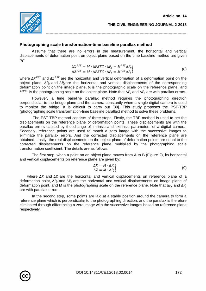
The number of sites suceptible to liquefaction with increase in earthquake maginitude is plotted in the Figure 11. By observing the Figure 11, it was noted that the majority of the locations in the region are liquefiable when the magnitude of quake exceeds 5. It was unequivocally distinguished that no site has indicated liquefaction vulnerability for a seismic quake for maginitude of 4. It can be inferred that the greater part of the capital region of Andhra Pradesh may not liquefiable when a light seismic quake happens.

Fig. 11. - Graph represents Earthquake magnitude and Number of sites liquefiable

CONCLUSION Liquefaction susceptibility assessment based on empirical approach with SPT value (N value)

was carried out at various places in capital of Andhra Pradesh state, India. The following conclusions were drawn from the analysis.

1. Liquefaction analysis should be carried for the all the structures and mainly for structures of national importance.

2. Many of the liquefaction susceptibility studies need to be considered in early stages of planning and design in order to select the most appropriate sites and also to improve sites for mitigating liquefaction susceptibility.

3. Liquefaction susceptibility assessment based SPT value is quite feasible. Since SPT was most widely used method soil exploration in India.

4. Most of the sites in the capital region of Andhra Pradesh are susceptible to liquefaction at the magnitude of earthquake 6 and above.

5. Majority of the sites of capital of Andhra Pradesh may not susceptible to liquefaction when a light earthquake happens. If a strong earthquake happens almost all the areas in the capital of Andhra Pradesh are susceptible to liquefaction and there is a chance of huge loss for life and property.

0

20

40

60

80

100

120

4 4,5 5 5,5 6 6,5 7 7,5

Nu

mb

er.

of

site

s li

qu

efia

ble

Earthquake Magnitude

Article no. 13


-----------------------------------------------------------------------------------------------------------------

DOI 10.14311/CEJ.2018.02.0013 167

6. The findings would help the designers in taking suitable decisions for design of foundations, resistant to liquefaction and to adopt appropriate ground improvement techniques for rapidly developing capital of Andhra Pradesh.

REFERENCES

[1] Kramer, S.L. “Geotechnical Earthquake Engineering”, Pearson Education (Singapore) Private Ltd., New

Delhi, 2003. [2] Sitharam, T.G., Govindaraju L. and Sridharan A. “Dynamic properties and liquefaction potential of soils”,

Special Section: Geotechnics and Earthquake Hazards, Current Science, 87(10), pp. 1370-1378, 2004. DOI: http://repository.ias.ac.in/83095/

[3] IS: 1893-Part 1. “Criteria for earthquake resistant design of structure –General provisions and buildings”. Bureau of Indian Standards, New Delhi, 2016.

[4] Cetin, K.O., Seed, R.B., Kiureghian, A.D., Tokimatsu, K., Harder, L.F. Jr., Kayen, R.E., and Moss,

R.E.S. “Standard penetration test-based probabilistic and deterministic assessment of seismic soil

liquefaction potential”. Journal of Geotechnical and Geoenvironmental Engineering, 12(1), pp. 1314-

1340. 2004. DOI: 10.1061/(ASCE)1090-0241(2004)130:12(1314)

[5] Seed, H.B., and Idriss, I.M. “Simplified procedure for evaluating soil liquefaction potential”, Journal of Soil Mechanics and Foundations Division, 97(9), pp. 1249-1273. 1971. DOI: http://cedb.asce.org/CEDBsearch/record.jsp?dockey=0018424

[6] Seed, H.B., Cetin, K.O., Moss, R.E.S., Kammerer, A.M., Wu, J., Pestana, J.M., Riemer, M.F., Sancio, R.B., Bray, J.D., Kayen, R.E. and Faris, A. “Recent Advances in Soil Liquefaction Engineering: A Unified and Consistent Frame work”, proc. of 26th annual ASCE Los Angeles Geotechnical Spring Seminar, pp. 1-71. 2003. DOI: http://digitalcommons.calpoly.edu/cgi/viewcontent.cgi?article=1007&context=cenv_fac

[7] Idriss, I.M. and Boulanger, R.W. “Evaluation of Liquefaction Potential, Consequences and Mitigation. Invited Expert Lectures”. Proc. Indian Geotechnical Conference-2005, pp. 3-25, 2005.

[8] Ramesh, N. and Suzuki, K. “Liquefaction Potential Analysis of Kathmandu Valley”, pp. 9-16, 2010. http//www.civil.saitama-u.ac.jp/content/files/2010neupane_suzuki.pdf

[9] Kumar, V.S. and Arumairaj, P.D. “Prediction of Liquefaction Potential of Soil for Coimbatore City Corporation Based on SPT Test Data”, Proc. of Indian Geotechnical Conference -2014, pp. 562-566, 2014.

[10] Bandyopadhyay, K., Bhattacharjee, S., Mitra, S., Ghosh, R. and Arnab K.P. “Determination of Liquefaction Potential of a Local Sub Soil by In-Situ Standard Penetration Test”. Proc. of Indian Geotechnical Conference 2014, pp. 567-571, 2014.

[11] Das, D. and Ghosh, A. “Liquefaction Analysis of Alluvial Soil Deposit”. Proc. of 50th Indian Geotechnical Conference, 2015. DOI: http://www.igs.org.in/igc-proceedings-2015/5/IGC-2015_submission_66.pdf

[12] Status: 05/2017, Edition No: 2, Facts & Figures, Andhra Pradesh Capital Region Development

Authority, Vijayawada, Andhra Pradesh – India. DOI:

https://crda.ap.gov.in/APCRDADOCS/DataModuleFIles/FACTS%20AND%20FIGURES%20OF%20CA

PITAL%20REGION/01~1117CRDA%20Factfile%20(%20Web%20view).pdf

[13] IS: 2131. “Method for standard penetration test for soils”, Bureau of Indian Standards, New Delhi, 1981. [14] Prakash, S. and Puri, V.K. “Past and Future of Liquefaction”, Proc. Indian Geotechnical Conference-

2010, pp.63-72. 2010. DOI: http//gndec.ac.in/~igs/ldh/conf/2010/articles/v008.pdf

http://repository.ias.ac.in/83095/

http://dx.doi.org/10.1061/(ASCE)1090-0241(2004)130:12(1314)

http://cedb.asce.org/CEDBsearch/record.jsp?dockey=0018424

http://digitalcommons.calpoly.edu/cgi/viewcontent.cgi?article=1007&context=cenv_fac

Article no. 14


---------------------------------------------------------------------------------------------------------------

DOI 10.14311/CEJ.2018.02.0014 168

MONITORING DYNAMIC GLOBAL DEFLECTION OF A BRIDGE BY MONOCULAR DIGITAL PHOTOGRAPHY

Guojian Zhang1, Guangli Guo1, Chengxin Yu2, and Long Li3,4

1. NASG Key Laboratory of Land Environment and Disaster Monitoring & School of Environmental

Science and Spatial Informatics, China University of Mining and Technology, Daxue Road 1,

221116 Xuzhou, Jiangsu, P.R. China; [email protected], [email protected]

(Corresponding author)

2. Business School, Shandong Jianzhu University, Fengming Road 1000, 250101 Jinan,

Shandong, P.R. China; [email protected]

3. School of Environmental Science and Spatial Informatics, China University of Mining and

Technology, Daxue Road 1, 221116 Xuzhou, Jiangsu, P.R. China; [email protected]

4. Department of Geography, Earth System Science, Vrije Universiteit Brussel, Pleinlaan 2, 1050

Brussels, Belgium; [email protected]

ABSTRACT

This study uses MDP (monocular digital photography) to monitor the dynamic global deflection of a bridge with the PST-TBP (Photographing scale transformation-time baseline parallax) method in which the reference system set near the camera is perpendicular to the photographing direction and does not need parallel to the bridge plane. A SONY350 camera was used to shoot the bridge every two seconds when the excavator was moving on the bridge and produced ten image sequences. Results show that the PST-TBP method is effective in solving the problem of the photographing direction being perpendicular to the bridge plane in monitoring the bridge by MDP. The PST-TBP method can achieve sub-pixel matching accuracy (0.3 pixels). The maximal deflection of the bridge is 55.34 mm which is within the bridge’s allowed value of 75mm. The MDPS (monocular digital photography system) depicts deflection trends of the bridge in real time, which can warn the possible danger of the bridge in time. It provides key information to assess the bridge health on site and to study the dynamic global deformation mechanism of a bridge caused by dynamic vehicle load. MDP is expected to be applied to monitor the dynamic global deflection of a bridge.

KEYWORDS

Monocular digital photography (MDP), Bridge health, Dynamic global deflection, Image sequences,Photographing scale transformation-time baseline parallax (PST-TBP) method

INTRODUCTION

Bridge deflection is an important basis to evaluate bridge health as it directly reveals the rigidity, stability, bearing capability and earthquake resistance of the bridge [1]. Bridge dynamic deflection can reflect the load impact coefficient and the internal force distribution of the structure [2]. It is therefore important to monitor the dynamic deflection of a bridge with a traffic light as it confronts heavier vehicle dynamic loads than others [3].






Article no. 14


---------------------------------------------------------------------------------------------------------------

DOI 10.14311/CEJ.2018.02.0014 169

At present, there are many methods to monitor bridge deflection such as the precise levelling, the total station, the measurement robot, the laser speckle, the photographic imaging, the inclinometer method, GPS (Global Positioning System), the inertial measurement, the tension line method, the pipe deflection monitoring method and the photogrammetric techniques. The precise levelling can monitor the static bridge deflection with high precision, it is however out of monitoring the dynamic bridge deflection [4]. The total station can be used to monitor the deflection of a long-span bridge. It is however challenging to monitor the bridge dynamic deflection [5]. Although the measurement robot can monitor the instantaneous coordinates of a single point, it only can monitor the short periodic deflection of the bridge as it continuously monitors the same point two times with a periodic [6]. The laser speckle and the photographic imaging can monitor the dynamic deflection of a point on the bridge without monitoring the dynamic global deflection of a bridge [7, 8]. The inclinometer can monitor the bridge dynamic deflection with high precision, but it requires the installation shaft parallel to the bridge axis which is difficult to carry out in the field [9]. GPS can be used to monitor a long-span bridge as it has a low accuracy in monitoring the dynamic deflection of a bridge [10]. The inertial measurement has a high-resolution ability, but it is ineffective in low frequency [11]. The tension line method cannot monitor the global dynamic deflection of a bridge as one tension line only can monitor the deflection of one point [12]. The pipe method can monitor the static global deflection of the bridge, but it is not flexible in monitoring the dynamic deflection of a bridge yet [13]. Photogrammetric techniques [14, 15] can monitor the global deflection of a bridge, and it has advantage in non-contact measuring. But it cannot monitor the dynamic global deflection of a bridge as it uses two cameras or takes images from at least two different positions by one camera [16].

As such, a specific method is required to monitor the dynamic global deflection of a bridge and warn the possible danger of the bridge in time. MDP offers the potential to solve this problem [17, 18]. MDP, combining close range photogrammetric technique [19-21] with information technology [22, 23], can monitor dynamic global deflection of a bridge and obtain image sequences of a bridge as it continuously monitors a bridge by a single digital camera. Although it has not been as popular in bridge structures as the photogrammetric techniques, many pioneering applications in this field have proved its increasing capability [24, 25].

It is clear that in most of the previous studies MDP had been used in monitoring bridge deflection. However, they did not consider problems such as digital camera parallaxes caused by the environment and the photographing direction being un-perpendicular to the bridge plan.

The aim of this study is to propose the PST-TBP (photographing scale transformation-time baseline parallax) method in MDP to monitor the dynamic global deflection of a bridge to grasp the deflection characteristics of the bridge caused by vehicle dynamic load and MDPS (monocular digital photography system) is used to depict the deflection trend curves of the bridge in real time to assess bridge health on site and warn the possible danger.

MONOCULAR DIGITAL PHOTOGRAPHY SYSTEM

Accuracy assessment of a digital camera

This study uses DLT (direct linear transformation) method to assess the digital camera accuracy [26]. Firstly, eight or more reference points with weights are properly distributed in the laboratory. Then, we used the indirect adjustment method to calculate the data with consideration

of L coefficients. The DLT method model is expressed as (1)：

Article no. 14


---------------------------------------------------------------------------------------------------------------

DOI 10.14311/CEJ.2018.02.0014 170

𝑥 −

𝐿1𝑋+𝐿2𝑌+𝐿3𝑍+𝐿4

𝐿9𝑋+𝐿10𝑌+𝐿11𝑍+1= 0

𝑧 −𝐿5𝑋+𝐿6𝑌+𝐿7𝑍+𝐿8

𝐿9𝑋+𝐿10𝑌+𝐿11𝑍+1= 0

} (1)

where x and z are image plane coordinates of deformation points without errors, X, Y and Z are the space coordinates of the correspondence deformation points, and Li (i =1,2,3,…,11) are the functions of the exterior and interior parameters of a digital camera.

The error (2) can be obtained by linearizing Equation (1):

𝑣 = (𝑃1𝑉1𝑃2𝑉2

) = (𝑀 𝑁00 𝐼

)(∆𝐿∆𝑋) − (𝑊1

0)

(2)

where P1 and P2 are the weight matrices of image point observations and the reference point observations, respectively, ∆𝑋 is the correction matrix of the reference points, N0 is the coefficient

matrix of ∆𝑋，M is the coefficient matrix of ∆𝐿 , and 𝑊1 is the constant matrix of image point

observations.

In Table 1, the calculation distances of U0-U2, U1-U3, and U2-U4 were obtained by the DLT method. Measurement distances of U0-U2, U1-U3, and U2-U4 were seen as precise values. The measurement errors were obtained by differencing the calculation distance with the corresponding measurement distance. The maximal measurement error of the digital camera is within 1mm which meets the accuracy requirements of deformation monitoring [27].

Tab. 1 - Measurement error/mm

Line U0-U2 U1-U3 U2-U4

Calculation distance 588 596 599

Measurement distance 589 595 599

difference 1 1 0

A principle of photographic scale transformation

The photographic scale of somewhere always changes along the photographing distance (from the position to the photography centre) [28, 29]. Figure 1 shows a schematic diagram of a CCD (Charge Coupled Device) camera capturing images at different photographing distances H3 and H4. H1 is the focal length of a CCD camera, H2 is the distance between the optical origin (o) and the front end of CCD camera, D1 on reference plane and D2 on object plane are the real-world length formed by the view field of the CCD camera at photographing distances H3 and H4 respectively, and N is the maximal pixel number in a horizontal scan line of an image plane, which is fixed and known as a priori irrelevant of the photographing distances.

Article no. 14


---------------------------------------------------------------------------------------------------------------

DOI 10.14311/CEJ.2018.02.0014 171

o

Image plane

CCD

Camera

Reference plane

H1

H2

H3

H4

N

D1

D2

Object plane

Fig. 1 - Schematic diagram of photographing scale transformation

Based on Figure 1, the relationship between pixel counts and distances can be described by:

𝐻1

𝐻2+𝐻3=

𝑁

𝐷1𝐻1

𝐻2+𝐻4=

𝑁

𝐷2

} (3)

In general, H3 and H4 are meter-sized, while H2 is centimetre-sized. Assume that H2 can be ignored when the camera is far from the bridge, Equation (3) can be expressed as:

𝐻1

𝐻3=

𝑁

𝐷1𝐻1

𝐻4=

𝑁

𝐷2

} (4)

From Equation (4), we have:

𝐷2 =𝐻4

𝐻3∙ 𝐷1 (5)

Assume that M1 and M2 are the photographing scale of the reference plane and the object plane, respectively. According to Equation (5), we have:

𝑀2 =𝐻4

𝐻3∙ 𝑀1 (6)

Namely,

𝑀2 = ∆𝑃𝑆𝑇𝐶 ∙ 𝑀1 (7)

where ∆𝑃𝑆𝑇𝐶 is the photographing scale transformation coefficient, and ∆𝑃𝑆𝑇𝐶 =𝐻4

𝐻3

Article no. 14


---------------------------------------------------------------------------------------------------------------

DOI 10.14311/CEJ.2018.02.0014 172

Photographing scale transformation-time baseline parallax method

Assume that there are no errors in the measurement, the horizontal and vertical displacements of deformation point on object plane based on the time baseline method are given by:

∆𝑋𝑃𝑆𝑇 = 𝑀 ∙ ∆𝑃𝑆𝑇𝐶 ∙ ∆𝑃𝑥 = 𝑀

𝑃𝑆𝑇∆𝑃𝑥∆𝑍𝑃𝑆𝑇 = 𝑀 ∙ ∆𝑃𝑆𝑇𝐶 ∙ ∆𝑃𝑧 = 𝑀

𝑃𝑆𝑇∆𝑃𝑧}

(8)

where 𝛥𝑋𝑃𝑆𝑇 and 𝛥𝑍𝑃𝑆𝑇 are the horizontal and vertical deformation of a deformation point on the object plane, ∆𝑃𝑥 and ∆𝑃𝑧 are the horizontal and vertical displacements of the corresponding deformation point on the image plane, M is the photographic scale on the reference plane, and

𝑀𝑃𝑆𝑇 is the photographing scale on the object plane. Note that ∆𝑃𝑥 and ∆𝑃𝑧 are with parallax errors.

However, a time baseline parallax method requires the photographing direction perpendicular to the bridge plane and the camera constantly when a single-digital camera is used to monitor the bridge. It is difficult to carry out [30]. This study proposes the PST-TBP (photographing scale transformation-time baseline parallax) method to solve these problems.

The PST-TBP method consists of three steps. Firstly, the TBP method is used to get the displacements on the reference plane of deformation points. These displacements are with the parallax errors caused by the change of intrinsic and extrinsic parameters of a digital camera. Secondly, reference points are used to match a zero image with the successive images to eliminate the parallax errors. And the corrected displacements on the reference plane are obtained. Lastly, the real displacements on the object plane of deformation points are equal to the corrected displacements on the reference plane multiplied by the photographing scale transformation coefficient. The details are as follows:

The first step, when a point on an object plane moves from A to B (Figure 2), its horizontal and vertical displacements on reference plane are given by:

∆𝑋 = 𝑀 ∙ ∆𝑃𝑥∆𝑍 = 𝑀 ∙ ∆𝑃𝑧

}

(9)

where ∆𝑋 and ∆𝑍 are the horizontal and vertical displacements on reference plane of a

deformation point, ∆𝑃𝑥 and ∆𝑃𝑧 are the horizontal and vertical displacements on image plane of deformation point, and M is the photographing scale on the reference plane. Note that ∆𝑃𝑥 and ∆𝑃𝑧 are with parallax errors.

In the second step, some points are laid at a stable position around the camera to form a reference plane which is perpendicular to the photographing direction, and the parallax is therefore eliminated through differencing a zero image with the successive images based on reference plane, respectively.

Article no. 14


---------------------------------------------------------------------------------------------------------------

DOI 10.14311/CEJ.2018.02.0014 173

C3

A

B

ΔXPST

ΔZPST

x

z

x

z

a

b

ΔPx

ΔPz

Image plane

Object plane

C0

S Projection center

Reference plane

C2

C4

C1

C5

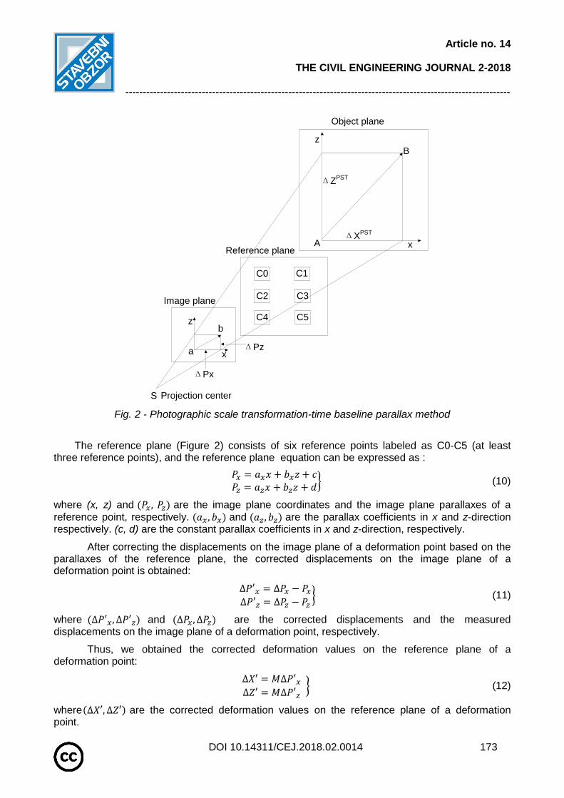
Fig. 2 - Photographic scale transformation-time baseline parallax method

The reference plane (Figure 2) consists of six reference points labeled as C0-C5 (at least three reference points), and the reference plane equation can be expressed as :

𝑃𝑥 = 𝑎𝑥𝑥 + 𝑏𝑥𝑧 + 𝑐𝑃𝑧 = 𝑎𝑧𝑥 + 𝑏𝑧𝑧 + 𝑑

}

(10)

where (x, z) and (𝑃𝑥 , 𝑃𝑧) are the image plane coordinates and the image plane parallaxes of a

reference point, respectively. (𝑎𝑥 , 𝑏𝑥) and (𝑎𝑧, 𝑏𝑧) are the parallax coefficients in x and z-direction respectively. (c, d) are the constant parallax coefficients in x and z-direction, respectively.

After correcting the displacements on the image plane of a deformation point based on the parallaxes of the reference plane, the corrected displacements on the image plane of a deformation point is obtained:

∆𝑃′𝑥 = ∆𝑃𝑥 − 𝑃𝑥∆𝑃′𝑧 = ∆𝑃𝑧 − 𝑃𝑧

}

(11)

where (∆𝑃′𝑥, ∆𝑃′𝑧) and (∆𝑃𝑥 , ∆𝑃𝑧) are the corrected displacements and the measured displacements on the image plane of a deformation point, respectively.

Thus, we obtained the corrected deformation values on the reference plane of a deformation point:

∆𝑋′ = 𝑀∆𝑃′𝑥∆𝑍′ = 𝑀∆𝑃′𝑧

}

(12)

where(∆𝑋′, ∆𝑍′) are the corrected deformation values on the reference plane of a deformation point.

Article no. 14


---------------------------------------------------------------------------------------------------------------

DOI 10.14311/CEJ.2018.02.0014 174

The last step is obtaining the corrected displacements on the object plane of a deformation point:

(∆𝑋𝑃𝑆𝑇)′ = ∆𝑃𝑆𝑇𝐶 ∙ ∆𝑋′

(∆𝑍𝑃𝑆𝑇)′ = ∆𝑃𝑆𝑇𝐶 ∙ ∆𝑍′}

13)

where (∆𝑋𝑃𝑆𝑇)′and (∆𝑍𝑃𝑆𝑇)′ are the corrected displacements on the object plane of a deformation point.

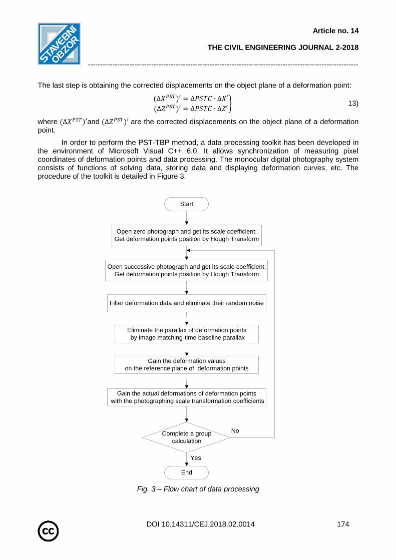
In order to perform the PST-TBP method, a data processing toolkit has been developed in the environment of Microsoft Visual C++ 6.0. It allows synchronization of measuring pixel coordinates of deformation points and data processing. The monocular digital photography system consists of functions of solving data, storing data and displaying deformation curves, etc. The procedure of the toolkit is detailed in Figure 3.

Start

Open successive photograph and get its scale coefficient;

Get deformation points position by Hough Transform

Filter deformation data and eliminate their random noise

Open zero photograph and get its scale coefficient;

Get deformation points position by Hough Transform

Eliminate the parallax of deformation points

by image matching-time baseline parallax

Gain the deformation values

on the reference plane of deformation points

Complete a group

calculation

End

Yes

NoGain the actual deformations of deformation points

with the photographing scale transformation coefficients

No

Fig. 3 – Flow chart of data processing

Article no. 14


---------------------------------------------------------------------------------------------------------------

DOI 10.14311/CEJ.2018.02.0014 175

BRIDGE TEST

Figure 4 shows an early stage of the Fenghuangshan road bridge which is a self-balanced reinforced concrete, central bearing frame arch. This bridge has a 60-meter span, and a 31.5meter march made of steel tube concrete. Its deck is equipped with motor vehicles, facilities, slow lane, sidewalks and guardrails.

Before the test, we set the total station and three digital cameras on the specified position of the south side of the Xiaoqing river. To facilitate the stress analysis of this bridge and the field condition, six deformation point targets labelled as U0-U5 were set on the bridge’s superstructure, and seven deformation point targets labelled as U6-U12 were evenly set on the bridge’s major deck. Reference points labelled as C0-C1, forming the reference system, were set near the digital camera whose view is in Figure 4. The reference system, used to match a zero image with the successive image, is perpendicular to the photographing direction.

Fig. 4 - Field test on the Fenghuangshan road bridge (taken on July 16, 2009)

In the bridge test, the SONY350 cameras were held constantly as much as possible. The cameras used in this test can capture the instantaneous deflection of a bridge in 1‰ second and shoot this bridge seven times in one second. The test process was described as follows:

(1) In the test, one excavator moved on the deck at a speed of 20km/h from the north to the south. The cameras were used to shoot the bridge to produce the zero images before the excavator on the bridge.

(2) The cameras were used to shoot the bridge every two seconds when the excavator was moving on the bridge. Finally, ten successive images were produced.

(3) The total station was used to obtain the spatial coordinates of reference points and deformation points after the test.

Table 2 shows the two-dimension coordinates of selected monitoring points and camera as the elevation can be ignored in the study.

Article no. 14


---------------------------------------------------------------------------------------------------------------

DOI 10.14311/CEJ.2018.02.0014 176

Tab. 2 - Spatial coordinates of selected monitoring points and camera

Name Camera C0 C1 C2 U6 U9 U12

X/m 8809.216 8806.411 8800.765 8806.206 8737.778 8748.484 8760.244

Y/m 14818.612 14820.39 14824.41 14824.41 14912.62 14867.6 14820.76

DATA PROCESSING AND ANALYSIS

Photographing scales of deformation points

Based on the photographing scale transformation, the photographing scales of U6, U9, and U12 can be expressed as:

𝑀𝑈6𝑃𝑆𝑇 = 𝑀0 ∙ ∆𝑃𝑆𝑇𝐶𝑈6



} (14)

where 𝑀𝑈6𝑃𝑆𝑇，𝑀𝑈9

𝑃𝑆𝑇 and 𝑀𝑈12𝑃𝑆𝑇 are the photographing scales of U6, U9 and U12 after the

photographing scale transformation，respectively; 𝑀0 is the photographing scale on the reference

plane; ∆𝑃𝑆𝑇𝐶𝑈6，∆𝑃𝑆𝑇𝐶𝑈9 𝑎𝑛𝑑 ∆𝑃𝑆𝑇𝐶𝑈12 are the photographing scale transformation coefficients of U6, U9, and U12, relative to the reference plane.

∆𝑃𝑆𝑇𝐶𝑈6，∆𝑃𝑆𝑇𝐶𝑈9 𝑎𝑛𝑑 ∆𝑃𝑆𝑇𝐶𝑈12 can be expressed as:

∆𝑃𝑆𝑇𝐶𝑈6 =𝑂𝐷

𝑂𝐴

∆𝑃𝑆𝑇𝐶𝑈9 =𝑂𝐶

𝑂𝐴

∆𝑃𝑆𝑇𝐶𝑈12 =𝑂𝐵

𝑂𝐴}

(15)

where OA, OB, OC, and OD are the photographing distances of the reference plane, U12, U9, and U6, relative to the camera. They are detailed in Figure 5.

Article no. 14


---------------------------------------------------------------------------------------------------------------

DOI 10.14311/CEJ.2018.02.0014 177

Reference system

U10U11

U12

C0

C1

Camera

Line 4

O

B

A

DBridge

U9

U8U7

U6

Line

3

Line 6

Lin

e 2

Line 1

Line 5

(C)

Fig. 5 - Illustration of the photographing scale transformation in the bridge test.

The photographing direction is perpendicular to the reference system, Line4, Line5, and Line6. Point A is the projection of Line 2 in reference system. Points B, C, and D are the intersections of Line 4 and Line 2, Line 5 and Line 2, Line 6 and Line 2, respectively. OB is the projection of Line1

in Line2 and OD is the projection of Line 3 in Line2.

Similarly, the approximate photographing scales of C0, C1, U7, U8, U10, and U11 were obtained. Table 3 shows the photographing scales of these reference points and deformation points on the bridge deck.

Tab. 3 - Photographing scales of C0-C1 and U6-U12/ (mm/pixel)

𝑀𝐶0 𝑀𝐶1 𝑀𝑈6𝑃𝑆𝑇 𝑀𝑈7

𝑃𝑆𝑇 𝑀𝑈8𝑃𝑆𝑇 𝑀𝑈9

𝑃𝑆𝑇 𝑀𝑈10𝑃𝑆𝑇 𝑀𝑈11

𝑃𝑆𝑇 𝑀𝑈12𝑃𝑆𝑇

1.65 1.65 28.93 25.86 22.79 19.70 17.51 15.32 13.14

Measurement accuracy

In theory, reference points did not move during the test and their displacements were zero. However, the displacements of these reference points obtained by the PST-TBP method were not zero. These displacement values of these reference points can therefore be used to represent the measurement accuracy. Table 4 shows that the maximal error is 1.65mm in monitoring the reference points.

As image matching is the key to this monocular digital photography, we measured the image coordinates of these deformation points on the zero image times to assess its image matching accuracy. Table 5 shows that the maximal error was 1 pixel, and the minimal error was 0 pixels. The average errors of U6-U12 were 0.1 pixels, 0.1 pixels, 0 pixels, 0.3 pixels, 0 pixels, 0.3 pixels and 0.2 pixels, respectively. This method reached a sub-pixel Image matching accuracy.

Article no. 14


---------------------------------------------------------------------------------------------------------------

DOI 10.14311/CEJ.2018.02.0014 178

Based on Table 3, it was obtained that the deflection errors of U6-U12 were 2.89 mm, 2.59 mm, 0 mm, 5.91 mm, 0 mm, 4.60 mm, 2.63 mm. The maximal and average deflection errors were 5.91 mm and 1.86 mm, respectively.

Tab. 4 - Measurement errors of reference points/mm

Point Test1 Test2 Test3 Test4 Test5 Test6 Test7 Test8 Test9 Test10

C0 0.00 0.00 0.00 1.65 1.65 0.01 0.00 0.00 0.00 0.01

C1 0.01 0.00 0.00 0.00 0.00 1.64 0.00 0.00 0.00 0.00

Tab. 5 - Image matching errors of deformation points/pixel

Test U6 U7 U8 U9 U10 U11 U12

1 1 0 0 0 0 1 0

2 0 0 0 1 0 0 1

3 0 0 0 1 0 0 0

4 0 0 0 1 0 1 0

5 0 0 0 0 0 1 0

6 0 0 0 0 0 0 1

7 0 0 0 0 0 0 0

8 0 0 0 0 0 0 0

9 0 1 0 0 0 0 0

10 0 0 0 0 0 0 0

Average 0.1 0.1 0 0.3 0 0.3 0.2

Analysis of bridge deflection trends

We calculated the pixel displacements (Table 6) and space displacements of some deformation points (Table 7). The positive and negative values (Tables 6 and 7) represent the deformation point moving up and down, respectively. The deformation points on the bridge deck (U6-U12) were chosen as the aim of this paper is to study the bridge deflection trends caused by vehicle dynamic load. Table 7 shows that in Test 6 deformation point U7 developed the maximal deflection-55.34 mm which was within the allowed value-75mm (the allowed value = the bridge span/800, where L = 60 m in this study).

Article no. 14


---------------------------------------------------------------------------------------------------------------

DOI 10.14311/CEJ.2018.02.0014 179

Tab. 6 - Pixel displacements of U6-U12/pixel

Test U6 U7 U8 U9 U10 U11 U12

1 -1.07 -0.76 -1.26 -0.44 -1.06 -1.53 -0.52

2 -1.18 -1.96 -1.65 -1.04 -0.88 -1.65 -1.21

3 -1.18 -0.95 -0.65 -1.03 -0.87 -0.65 -1.20

4 -0.18 -0.95 -0.65 -1.03 -0.88 -1.65 -1.19

5 -0.53 0.46 -0.46 -0.12 -0.35 -1.71 -1.24

6 -1.28 -2.14 -2.02 -1.60 -1.68 -1.76 -1.86

7 -1.17 -0.95 -1.64 -1.03 -0.87 -1.65 -0.20

8 -0.62 -0.72 -0.82 -0.68 -2.15 -1.81 -1.89

9 -0.18 0.04 -0.65 -1.03 -0.87 -0.65 -1.20

10 -1.17 -0.96 -0.64 -1.02 -0.87 -0.65 -1.19

Tab. 7 - Space displacements of U6-U12/mm

Test U6 U7 U8 U9 U10 U11 U12

1 -30.96 -19.65 -28.72 -8.67 -18.56 -23.44 -6.83

2 -34.14 -50.69 -37.60 -20.49 -15.41 -25.28 -15.90

3 -34.14 -24.57 -14.81 -20.29 -15.23 -9.96 -15.77

4 -5.21 -24.57 -14.81 -20.29 -15.41 -25.28 -15.64

5 -15.33 11.90 -10.48 -2.36 -6.13 -26.20 -16.29

6 -37.03 -55.34 -46.04 -31.52 -29.42 -26.96 -24.44

7 -33.85 -24.57 -37.38 -20.29 -15.23 -25.28 -2.63

8 -17.94 -18.62 -18.69 -13.40 -37.65 -27.73 -24.83

9 -5.21 1.03 -14.81 -20.29 -15.23 -9.96 -15.77

10 -33.85 -24.83 -14.59 -20.09 -15.23 -9.96 -15.64

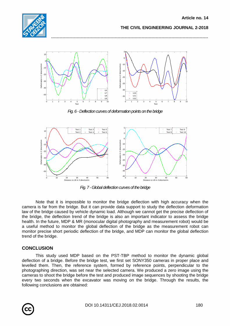
Deflection curves (Figures 6 and 7) were also depicted in order to visually analyse the bridge deflection law caused by vehicle dynamic load. Figure 6 shows that the deflection of every

position on the bridge’s major structure was inelastic, all of which was within the bridge allowed value. Figure 7 shows that vehicle dynamic load results in the bridge moving down in spite of U7 moving up in test 5 and 7. In addition, the bridge global deflection curves fluctuated up and down like some sinusoidal-cosinusoidal curves. The bridge deflection was a parabola when the excavator moved to the bridge centre (Test 6). Especially, the deflection of every position on the bridge almost reached its maximal when the excavator moved to the bridge centre, which conforms to the deformation characteristics of the bridge caused by the external load.

Article no. 14


---------------------------------------------------------------------------------------------------------------

DOI 10.14311/CEJ.2018.02.0014 180

Fig. 6 - Deflection curves of deformation points on the bridge

Fig. 7 - Global deflection curves of the bridge

Note that it is impossible to monitor the bridge deflection with high accuracy when the camera is far from the bridge. But it can provide data support to study the deflection deformation law of the bridge caused by vehicle dynamic load. Although we cannot get the precise deflection of the bridge, the deflection trend of the bridge is also an important indicator to assess the bridge health. In the future, MDP & MR (monocular digital photography and measurement robot) would be a useful method to monitor the global deflection of the bridge as the measurement robot can monitor precise short periodic deflection of the bridge, and MDP can monitor the global deflection trend of the bridge.

CONCLUSION

This study used MDP based on the PST-TBP method to monitor the dynamic global deflection of a bridge. Before the bridge test, we first set SONY350 cameras in proper place and levelled them. Then, the reference system, formed by reference points, perpendicular to the photographing direction, was set near the selected camera. We produced a zero image using the cameras to shoot the bridge before the test and produced image sequences by shooting the bridge every two seconds when the excavator was moving on the bridge. Through the results, the following conclusions are obtained:

0 1 2 3 4 5 6 7 8 9 10

-50

-40

-30

-20

-10

0

10

Test

Defo

rmation in Z

direction/m

m

U6

U7

U8

U9

0 1 2 3 4 5 6 7 8 9 10

-35

-30

-25

-20

-15

-10

-5

0

Test

Defo

rmation in Z

direction/m

m

U10

U11

U12

0 10 20 30 40 50 60

-50

-40

-30

-20

-10

0

10

Defo

rmation in Z

direction/m

m

Distance to U6 in X direction/m

Test 1

Test 2

Test 3

Test 4

Test 5

Test 6

0 10 20 30 40 50 60-40

-35

-30

-25

-20

-15

-10

-5

0

5

Defo

rmation in Z

direction/m

m

Distance to U6 in X direction/m

Test 7

Test 8

Test 9

Test 10

Article no. 14


---------------------------------------------------------------------------------------------------------------

DOI 10.14311/CEJ.2018.02.0014 181

(1) The PST-TBP method reaches a sub-pixel image matching accuracy. The average image matching error was within 0.3 pixels. And the maximal error was 1.65mm and 5.91 mm in monitoring the reference points and dynamic global deflection of a bridge, respectively.

(2) Every position of the bridge almost reaches the maximal deflection when the excavator moves to the bridge centre. The maximal deflection of the bridge was 55.34mm which was within the bridge allowed value-75mm.

(3) The deflection curves of the bridge fluctuated up and down like some sinusoidal-cosinusoidal curves. The bridge deflection was a parabola when the excavator moved to the bridge centre.

(4) Deflections of every position on the bridge were inelastic, all of which was within the bridge allowed. This indicates that the bridge is in good health.

The MDPS (monocular digital photography system) used in this study can monitor the dynamic global deflection of a bridge. Deflection trends of the bridge depicted by this system in real time show the bridge deflection visually, which is effective in warning the possible danger of the bridge. Although it cannot get the precise bridge deflection when the camera is far from the bridge, the dynamic deflection trend of the bridge is also an important indicator to assess the bridge health. In the future, MDP & MR (monocular digital photography and measurement robot) would be a useful method to monitor the bridge deflection as it can get precise short periodic deflection deformation of the bridge and the dynamic global deflection trend of the bridge.

ACKNOWLEDGEMENTS

This study was supported by the National Natural Science Foundation of China (Grant No.: 51674249), the Science and Technology project of Shandong province of China (Grant No.: 2010GZX20125).

REFERENCES

[1] X. M. Hou, X. S. Yang, Z. P. Liao, and S. L. Ma, "Bridge deflection real time measurement,"

Earthquake Engineering & Engineering Vibration, vol. 22, pp. 67-72, 2002.

[2] X. L. He and L. Z. Zhao, "Based on Inclinometer to Measure Dynamic Deflection of High-Speed

Railway Bridge," Applied Mechanics & Materials, vol. 405-408, pp. 3019-3026, 2013.

[3] I. Lipták, A. Kopáčik, J. Erdélyi, and P. Kyrinovič, "Dynamic Deformation Monitoring of Bridge

Structure," Selected Scientific Papers - Journal of Civil Engineering, vol. 8, pp. 13-20, 2013.

[4] D. H. Parker, B. Radcliff, and J. W. Shelton, "Advances in hydrostatic leveling with the NPH6, and

suggestions for further enhancements," Precision Engineering, vol. 29, pp. 367-374, 2005.

[5] K. Y. Koo, J. M. W. Brownjohn, D. I. List, and R. Cole, "Structural health monitoring of the Tamar

suspension bridge," Structural Control & Health Monitoring, vol. 20, pp. 609–625, 2013.

[6] P. A. Psimoulis and S. C. Stiros, "Measuring Deflections of a Short-Span Railway Bridge Using a

Robotic Total Station," Journal of Bridge Engineering, vol. 18, pp. 182-185, 2013.

[7] Z. Xia, F. U. Hong qiao, W. Zhang, W. M. Chen, and Chongqing, "Modulation Transfer Function of

Image Monitoring System for Bridge's Deformation," Journal of Chongqing University, 2004.

[8] H. Dong, W. M. Chen, F. U. Yu mei, and Chongqing, "Method of laser & imaging deflection

measurement," Journal of Transducer Technology, 2004.

[9] X. Hou, X. Yang, and Q. Huang, "Using Inclinometers to Measure Bridge Deflection," Bridge

Construction, vol. 10, pp. 564-569, 2004.

[10] V. Ashkenzai and G. W. Roberts, "EXPERIMENTAL MONITORING OF THE HUMBER BRIDGE

USING GPS," in Institution of Civil Engineers: Civil Engineering, 1997, pp. 177-182.

Article no. 14


---------------------------------------------------------------------------------------------------------------

DOI 10.14311/CEJ.2018.02.0014 182

[11] Y. Xie, "Inertial Measurement Method for Railway Bridge Dynamic Deflection," Chinese Journal

Ofentific Instrument, 1999.

[12] J. F. Stanton, M. O. Eberhard, and P. J. Barr, "A weighted-stretched-wire system for monitoring

deflections," Engineering Structures, vol. 25, pp. 347-357, 2003.

[13] Y. Liu, Y. Deng, and C. S. Cai, "Deflection monitoring and assessment for a suspension bridge using

a connected pipe system: a case study in China," Structural Control & Health Monitoring, vol. 22, pp. 1408-

1425, 2015.

[14] M. A. R. Cooper and S. Robson, "HIGH PRECISION PHOTOGRAMMETRIC MONITORING OF THE

DEFORMATION OF A STEEL BRIDGE," Photogrammetric Record, vol. 13, pp. 505-510, 2006.

[15] C. Forno, S. Brown, R. A. Hunt, A. M. Kearney, and S. Oldfield, "Measurement of deformation of a

bridge by Moire photography and photogrammetry," Strain, vol. 27, pp. 83-87, 2008.

[16] H. G. Maas, "Photogrammetric techniques for deformation measurements on reservoir walls," 1998.

[17] Y. H. Yu, C. Vo-Ky, S. Kodagoda, and Q. P. Ha, "FPGA-Based Relative Distance Estimation for

Indoor Robot Control Using Monocular Digital Camera," vol. 14, pp. 714-721, 2010.

[18] V. Gorbatsevich, Y. Vizilter, V. Knyaz, and S. Zheltov, "Face Pose Recognition Based on Monocular

Digital Imagery and Stereo-Based Estimation of its Precision," International Archives of the Photogrammetry

Remote Sensing & S, vol. XL-5, pp. 257-263, 2014.

[19] R. R. P. D. Samuel, close-range photogrammetry: Springer Berlin Heidelberg, 2014.

[20] F. B. Bales, "CLOSE-RANGE PHOTOGRAMMETRY FOR BRIDGE MEASUREMENT,"

Transportation Research Record, vol. 1, 1984.

[21] K. Leitch, "CLOSE-RANGE PHOTOGRAMMETRIC MEASUREMENT OF BRIDGE

DEFORMATIONS," https://www.lap-publishing.com/, 2010.

[22] F. Remondino, "Image Sequence Analysis For Human Body Reconstruction," Archives of P & Rs,

vol. 34, pp. 590--595, 2002.

[23] N. D'Apuzzo, "Surface measurement and tracking of human body parts from multi-image video

sequences," ISPRS Journal of Photogrammetry and Remote Sensing, vol. 56, pp. 360-375, 8// 2002.

[24] S. Yoneyama, A. Kitagawa, S. Iwata, K. Tani, and H. Kikuta, "BRIDGE DEFLECTION

MEASUREMENT USING DIGITAL IMAGE CORRELATION," Experimental Techniques, vol. 31, pp. 34–40,

2007.

[25] P. Olaszek, "Investigation of the dynamic characteristic of bridge structures using a computer vision

method," Measurement, vol. 25, pp. 227-236, 1999.

[26] A. Goktepe and E. Kocaman, "Using Direct Linear Transformation Method in X-Ray Photogrammetry

and an Illustrative Study," Experimental Techniques, vol. 36, pp. 21–25, 2012.

[27] "Study of the Bridge Deformation Monitoring Technique and its Survey Specification," Marine

Environment & Engineering, 2011.

[28] M. C. Lu, C. C. Hsu, and Y. Y. Lu, "Distance and angle measurement of distant objects on an oblique

plane based on pixel variation of CCD image," in Instrumentation and Measurement Technology Conference

(I2MTC), 2010 IEEE, 2010, pp. 318 - 322.

[29] C. C. J. Hsu, M. C. Lu, and Y. Y. Lu, "Distance and Angle Measurement of Objects on an Oblique

Plane Based on Pixel Number Variation of CCD Images," IEEE Transactions on Instrumentation &

Measurement, vol. 60, pp. 1779-1794, 2010.

[30] C. Mingzhi, Y. ChengXin, X. Na, Z. YongQian, and Y. WenShan, "Application study of digital

analytical method on deformation monitor of high-rise goods shelf," in 2008 IEEE International Conference

on Automation and Logistics, 2008, pp. 2084-2088.

http://www.lap-publishing.com/

Article no. 15


---------------------------------------------------------------------------------------------------------------

DOI 10.14311/CEJ.2018.02.0015 183

DOUBLE SIZE FULLJET FIELD RAINFALL SIMULATOR FOR COMPLEX INTERRILL AND RILL EROSION STUDIES

Petr Kavka, Luděk Strouhal, Barbora Jáchymová, Josef Krása, Markéta Báčová, Tomáš Laburda, Tomáš Dostál, Jan Devátý and Miroslav Bauer

The Czech Technical University in Prague, Faculty of Civil Engineering, Department

of Irrigation, Drainage and Landscape Engineering, Prague,Thákurova 7, 16629,

Czech Republic; [email protected]

ABSTRACT

Field observations and consecutive modelling of soil erosion events proved to be essential for understanding and predicting erosion and sediment transport. An experimental approach often utilizes a large variety of rainfall simulators. In this technical note a complex methodology is introduced, using a mobile rainfall simulator developed at the Czech Technical University in Prague. An experimental setup with two watered plots (16 + 1 m2) was established, which enables simultaneous measurements in two scales and monitoring of surface runoff, flow velocity, infiltration, sediment subsurface flow, vegetation cover effect suspended solids and phosphorus transport, surface roughness and surface evolution under rainfall and other variables. The simulator is built on a trailer transportable by car with folding arm carrying four FullJet WSQ nozzles operating independently. The configuration and water pressure 0.7 bar leads to the total watered area 2.4 x 9.6 m. Average drop size (d50) reaches 1.75 mm for 0.7 bar pressure. Christiansen uniformity index CU reaches 85%. A selection of experimental results highlights both the advantages and the weaknesses of the presented experimental setup.

KEYWORDS Rainfall simulation, Surface runoff, Subsurface runoff, Mobile rainfall simulator

INTRODUCTION

Water erosion is the most widespread form of soil degradation. Reducing the erosion is one of the major challenges in landscape management. Sediment transport from arable land into surface waters (streams, rivers, reservoirs) induces many significant problems in water bodies [1]. This problem was highly accelerated when the landscape patterns were destructed during technical improvement of agro technology and land consolidations. In Eastern Europe this effect was accelerated by collectivization of agriculture [2]. Based on research it is known that sediment transport can be reduced by inhibition of the surface runoff and proper agricultural management.

Rainfall simulation experiments are widely used as a method to study various flow and transport processes induced by rainfall [3]. They have been used on different land uses, slopes, scales, soils and climate conditions [4], [5], [6]. But most of the experiments have been driven by rather narrow objectives and therefore do not provide data for complex description of rainfall runoff and sediment transport processes. That is one of the actual scientific objectives nowadays - to describe the driving mechanisms of the physical processes in details and consequently to implement the plot scale data in optimization of the catchment scale parameters.

Article no. 15


---------------------------------------------------------------------------------------------------------------

DOI 10.14311/CEJ.2018.02.0015 184

Surface runoff rate and sediment yield in the form of suspended solids concentration are standard variables observed in experiments oriented on soil erosion research with use of rainfall simulators. The review of small portable simulators used across Europe provides [7]. Due to the nature of the device the small simulators with watered area around 1 m2 are more frequent. Larger simulators can be found as well [8], [9], [10], [11]. They are essential for a consequent mathematical modelling of both surface and subsurface runoff and related processes.

Together with eroded soil particles various nutrients are transported in the surface runoff. Phosphorus is the most significant and monitored particulate nutrient in the environment [12], [13]. It enters the water courses and is retained in the ponds and water dams where it impairs the environmental balance and water quality [14].

Another runoff component is the quick subsurface flow also known as hypodermic flow or interflow [15]. On the arable land it mostly occurs on the interface between the shallow ploughed topsoil and compacted subsoil. Since these two flow components may interact and lead to implications for both erosion and hydrologic response to the rainfall event, it is important to observe and model the subsurface processes as well.

Soil erosion intensity (in particular splash type) is decreased with the vegetation growth [16]. The soil surface is protected largely due to the plant’s leaves, which absorb part of the kinetic energy of the raindrops. Farming operations also directly affect soil movement through activities such as tillage [17], root crop harvesting, and the trampling of soil and removal of vegetation by livestock. Combination of the current state of vegetation and farming operations influenced state of soil aggregates. Soil aggregates are less exposed to the direct impact of the raindrops and associated crumbling, which is considered as a trigger of the erosion process [18]. In order to evaluate the effect of the vegetation on particular soil erosion event it is therefore necessary to document the actual leaves extent. To this end two most common parameters are used: Canopy Cover and Leaf Area Index (LAI). Repetitions of the experiments in the same site during the growing season as well as comparing results from vegetated and bare experimental plots enable the vegetation cover and state of the soil surface effects to be assessed.

Together with detaching soil particles from the aggregates by the impact of raindrops also the surface runoff plays an important role in soil erosion, in particular its volume and flow velocity. Higher velocity induces larger shear stress and dragging forces to carried soil particles. From the known particle-size distribution of the eroded material basic physical principles of soil erosion can be verified [19].

METHODS

Device and setup description

Mobile rainfall simulator operated by CTU in Prague was constructed in 2012 in cooperation with Research Institute for Soil and Water Conservation (VÚMOP). Its detailed description can be found in [20] and only basic information will be given here. The essential part of simulator is a folding boom with four nozzles by Spraying Systems – FullJet 40WSQ [10] controlled by electromagnetic valves. The boom consists of a dural steel framed structure and eight supporting telescopic legs. The boom can be folded out directly from the trailer and heaved by a pulley into desired height. Once the legs are joined it is completely standalone and can be detached and moved independently, constrained only by the length of the control wires and water supplying hosepipes. The whole construction was designed to be easily and quickly set out and packed back again without any interfering with the plot marked for the simulation. In order to prevent the wind from affecting the simulation the supporting construction is covered with the tarpaulin.

Article no. 15


---------------------------------------------------------------------------------------------------------------

DOI 10.14311/CEJ.2018.02.0015 185

The device includes a 1 m3 tank, portable generator, pump producing a constant pressure with minimum delivery 40 l/min and a control unit for managing the rainfall intensity by triggering the electromagnetic valves. The electromagnetic valves trigger the separate pairs of nozzles. Their opening and closing in an arbitrary time interval produces the desired intensity of simulated rainfall. Coupling the nozzles into pairs reduces hydraulic shocks in the water distribution system and therefore helps maintaining a uniform spatial distribution of water over the experimental plot.

Four nozzles FullJet 40WSQ are positioned 2.65 m above the ground and 2.4 m apart. Type of the nozzles as well as the position were selected after many calibration tests aimed at reaching as uniform spatial distribution and droplet characteristics as similar to natural raindrops as possible. These tests were carried out on the plot 2.1 x 2.8 m centred under the first nozzle (for exact position see Figure 1), assuming that the rest of the area is symmetric. Final configuration yielded the Christiansen’s uniformity index [21] of 80% and more for all rainfall scenarios commonly used in the field simulations.

This configuration and water pressure 0.7 bar leads to the total watered area 2.4 x 9.6 m. It can be used for variable setup of experimental plots, although limited by decreasing rainfall intensity towards the edges of the watered area. In CTU simulations there are two separate plots used simultaneously, one with dimensions 1 x 1 m and another 2 x 8 m with the longer edge along the slope, as illustrated in Figure 1.

Fig. 1 - Scheme of the rainfall simulator with two plots and with position of the nozzles, rain gauge and soil moisture probe.

Rainfall characteristics

The most crucial variable influencing the course of the simulations are the rainfall intensity (spatial distribution and average over the plot) and droplet characteristics. Droplet size and impact velocity were analysed by a disdrometer, spatial distribution of intensity by a network of small buckets [22]. Average drop size (d50) reaches 1.75 mm for 0.7 bar pressure. Christiansen uniformity index CU [23] reaches 85%.

Article no. 15


---------------------------------------------------------------------------------------------------------------

DOI 10.14311/CEJ.2018.02.0015 186

In order to maintain uniform spatial distribution of water over the plots, the experimental setup was designed with rather large overspray of the experimental plots. Therefore only part of the sprinkled water falls onto the plots and a final intensity needs to be checked in each simulation.

First the outflow rate at the nozzles is checked by collecting and weighing the sprinkled water in a four minutes test, as it differs slightly depending on the exact water pressure in the system. Next a reference measurement is performed at the beginning of every campaign on the fallow plots covered with an impervious tarpaulin. The rainfall intensity is derived from the total discharge after the steady state is reached. From the acquired values from a whole set of campaigns a calibration curve describing the relationship between the outflow at the nozzles and resulting intensity onto the plots is being derived and consecutively refined. The curve is then used for rainfall intensity determination in simulations on the vegetated plots.

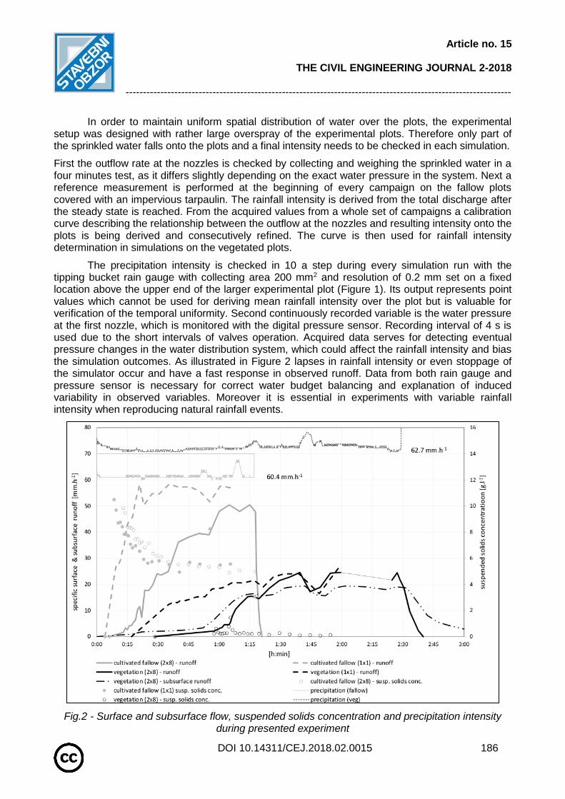
The precipitation intensity is checked in 10 a step during every simulation run with the tipping bucket rain gauge with collecting area 200 mm2 and resolution of 0.2 mm set on a fixed location above the upper end of the larger experimental plot (Figure 1). Its output represents point values which cannot be used for deriving mean rainfall intensity over the plot but is valuable for verification of the temporal uniformity. Second continuously recorded variable is the water pressure at the first nozzle, which is monitored with the digital pressure sensor. Recording interval of 4 s is used due to the short intervals of valves operation. Acquired data serves for detecting eventual pressure changes in the water distribution system, which could affect the rainfall intensity and bias the simulation outcomes. As illustrated in Figure 2 lapses in rainfall intensity or even stoppage of the simulator occur and have a fast response in observed runoff. Data from both rain gauge and pressure sensor is necessary for correct water budget balancing and explanation of induced variability in observed variables. Moreover it is essential in experiments with variable rainfall intensity when reproducing natural rainfall events.

Fig.2 - Surface and subsurface flow, suspended solids concentration and precipitation intensity during presented experiment

Article no. 15


---------------------------------------------------------------------------------------------------------------

DOI 10.14311/CEJ.2018.02.0015 187

Surface runoff and plot scale effect

Time to initiation of the surface runoff is determined visually by observing the discharge from the plot in the lower outlet. The runoff rate is measured in situ gravimetrically for variable time intervals. Within first 10 minutes after the runoff initiation the interval is 1 minute, another 10 minutes the runoff rate measurements are performed in 2 minute intervals and for the rest of the simulation (until 1 hour after the runoff initiation or reaching steady state) the interval is increased to 5 minutes. The purpose of this arrangement is to capture the dynamics of the runoff rate and suspended solids concentration. They change considerably within the initial phase and tend to steady in the course of the simulation, as shown in Figure 2.

The runoff needs to be measured independently for each of the two parallel plots. However the discharges are measured in the same intervals and samples are taken at the same relative time with respect to corresponding times of initiation. This way the runoff dynamics in both plots (1m2 and 16 m2) can be compared.

Soil water regime and shallow subsurface flow

The runoff monitoring is accompanied with soil water regime monitoring. The soil water content is measured in two ways. Undisturbed 100 cm3 soil samples are taken both before and after the simulation and later they are analysed in the lab. The soil water regime in the top 5 cm of the soil profile is continuously monitored with the ThetaProbe ML2x and recorded in 1 minute interval. Additional probes are installed in the depths of 30 cm and 50 cm below the surface.

To monitor shallow subsurface runoff a trench is being excavated along the lower edge of the larger experimental plot. It is 2 m long and 0.6 m deep. At the bottom of the trench a drainage pipe with diameter of 100 mm is installed. Both the bottom and the walls of the trench from the topsoil / subsoil divide below are covered with an impermeable plastic foil so that only shallow runoff from the topsoil reaches the drainage pipe. The trench is partly filled with the gravel and enclosed by the topsoil. The drainage pipe is connected through the collection pipes to a tipping bucket, where the subsurface runoff is continuously measured or sampled. The collection system was designed in a way which does not require removing prior to each agrotechnical operation.

Maximum flow velocity

For the flow velocity determination, two methods are used in parallel. For the maximum flow velocity which corresponds to the rillflow in the preferential flow paths the progress of the dye tracer Brilliant Blue FCF is observed. This method is especially used on the cultivated fallow plots. From the top of the plot the time intervals are measured for the tracer to travel each 1 m distance. In order to highlight the head of the moving tracer an extra dose of the dye is added at the beginning of each 1 m section. This measurement is repeated three times for each simulation after reaching the steady outflow and ideally close to the moments when the suspended soils samples are taken. The timing is important for the verification of the relationships between flow velocity and the grain size of suspended particles.

Average flow velocity

The dye tracer method is partially subjective due to the need of visual tracing and it is hard to use in case the surface is covered with full-grown vegetation. Besides the maximum flow velocity the mean velocity represents the process of sediment transport. This variable is obtained by measuring the electric conductivity after the application of potassium bromide (KBr) or sodium chloride (NaCl) solution. It is usually applied subsequently in 2, 4 and 6 meters from the lower end of the plot, so it is possible to derive the velocities in separate sections of the sloping plot. Using a conductometer (WTW Cond 3310) the beginning of the rise and the time of the peak of the conductivity wave is observed. Due to normally very long recession limb of the conductivity wave this measurement is being stopped once a distinct lapse in conductivity is observed. Beside the

Article no. 15


---------------------------------------------------------------------------------------------------------------

DOI 10.14311/CEJ.2018.02.0015 188

difficult manipulation (conflict with other measurements) another disadvantage of this method is a slow yet unwanted soil salinization which might in the long term lead to the inhibition of vegetation growth and impairing the soil fauna in the location.

Suspended solids

In order to evaluate the dynamics of suspended solids concentration the runoff samples are taken in the same time intervals as in the runoff rate measurements. The samples are weighed in the field and later analysed in the laboratory according to the standards [24]. Suspended solids are filtered from the solution, dried and their weight is converted into concentrations. Final sediment yield results from relation of concentrations to the runoff rates in respective time intervals of sampling.

Along with the samples for concentration analysis another set of samples is taken for determining the particle-size distribution. Since such determination is rather time-consuming, these samples are taken in 10 minute interval only. Based on results of particle-size analysis the changes in sediment composition during the erosion event may be monitored. When related to the runoff velocity the particle-size may also be used for determination of friction and dragging forces in the overland flow.

Phosphorus transport

Concerning the chemicals the phosphorus is monitored. Phosphorus concentration analyses are carried out on mixed samples composed of several 50 ml of runoff taken at different times. Resulting 5 samples represent three 5 minute and two 15 minute intervals of runoff. There are two basic forms of phosphorus in surface runoff: particle-bound and dissolved phosphorus. Mixed samples are stabilized in the field with highly concentrated HNO2 (0.5 ml HNO2 in 100 ml of sampled water) in order to avoid dissolved phosphorus decay. Later in the laboratory two types of samples are analysed using ICP-OES, Inductively coupled plasma optical emission spectrometry [25]. In the original unfiltered samples the total phosphorus concentration is determined. For dissolved phosphorus determination the suspended solids are removed from the samples using 0.45 µm filter. The particle-bound phosphorus is determined then as the dissolved phosphorus subtracted from the total.

Vegetation stage and soil protection

Leaf Area Index

LAI is measured within the LAI-2000 Plant Canopy Analyzer. The device is based on comparison of the light intensities above the vegetation and near the soil surface. Advantage of this method is that it is fast and enables repetitive or multiple measurements for obtaining a representative value. The measurement is always performed on the vegetated experimental plot and in the open crop field next to it. The value from the latter site serves as a reference value for detecting significant variance in the vegetation growth in the experimental plot due to previous simulations.

Canopy Cover

The measurement of CC is performed by sensing of the surface with the camera and analysing the images using a supervised classification in GIS software. The analysed plot is delimited with a metal squared frame of the area 1 m2, which is used for referencing and scaling of pictures.

Soil Loss Ratio (SLR)

The sheltering effect of the vegetation is quantified with use of Soil Loss Ratio (SLR). It is determined by referencing the sediment yield from the vegetated plot to the sediment yield from a

Article no. 15


---------------------------------------------------------------------------------------------------------------

DOI 10.14311/CEJ.2018.02.0015 189

standard, reference plot maintained as a fallow with seedbed conditions. The reference fallow is cultivated before each simulation according to the procedures stated in the technical standard [26]. First, the topsoil is ploughed into the depth of about 10 cm, aggregates loosened with the rake and levelled with the wooden batten. Large stones and remains of the plants are removed and at the end the surface is carefully rolled with a manual turf roller. Main goal of these procedures is to ensure the surface conditions as close to the reference state as possible for every simulation.

Soil surface roughness and surface changes

The soil surface changes and roughness are evaluated by a photogrammetric technique. The accuracy of derived surface representation depends on the camera specifications. The plausible spatial resolution is about 1-2 mm as reported e.g. in [27] and height accuracy compared to more precise laser scanning may be below 2 mm for smooth surfaces, as reported in [28]. Photogrammetric evaluation is based on the stereo imaging of the field plot surface before and after the rainfall simulation. Since the ground control points (GCPs) are necessary for the image referencing, a dural reference frame with 40 equally distributed GCPs was designed. The frame encloses the maximum area of 1.6 x 1.1 m and is equipped with a mobile cross bar labelled by GCPs which makes the size of the evaluated frame variable. The reference frame is kept in horizontal position with four threaded rods driven into the plot before the rainfall simulation. Sony NEX-5N, interchangeable lens Compact System Camera is utilized for the sensing. The reference frame is removed before the simulation start, whereas the rods are left in the plot to allow the frame being put in the same position after the simulation end. Photographs are always taken with the same camera settings (aperture f-8, exposure time 1/40 and less, focal length 16 or 18 mm depending on selected lens). Thanks to the tarpaulin covering the rainfall simulator the lighting has a diffuse character, which makes the sensing less sensitive to the changes in cloudiness and direct sunlight. The images are taken manually with camera oriented vertically in the height of approximately 1.3 m above the ground and the image distance of 0.3 m. Each captured photo covers the whole frame area and all reference points. Usually more than one stereo pair images are taken for providing larger sample for the evaluation.

Obtained stereo pair images are processed in PhotoModeler Scanner software, which derives accurate, high quality 3D models and enables measurements based on photographs. The process is known as photo-based 3D scanning [29] or image-based modelling [30] and is used for producing a dense point cloud (Dense Surface Modelling) from images of textured surfaces. The multi-sheet camera calibration is executed before the automatic Dense Surface Modelling.

Subsequently, dense surface point clouds created with PhotoModeler Scanner are processed in ArcGIS software. At first the digital surface model (DSM) is generated in the form of triangulated irregular network (TIN) which is then converted to a 1 mm raster DSM. Then the surface raster DSMs created before and after the rainfall simulation are subtracted. This subtraction is used in evaluation of soil volume replacement caused by the rainfall-runoff process. Other analyses are performed on the derived DSMs in order to quantify soil surface roughness parameters such as random roughness, tortuosity, mean upslope depression or other indices. The soil volume replacements as well as the roughness and surface indices are valuable for validation of physically based runoff and erosion models.

SELECTED 2014 STUDY RESULTS

A selection of typical outputs from CTU rainfall simulations is presented. Full results and their in-depth analysis are out of scope of this technical note, provided outputs are to illustrate the most important variables and phenomena discussed in previous sections. During an experimental campaign in June 26th 2014 the rainfall simulation was carried out on two parallel experimental plots in Bykovicky stream catchment. The field is located in Central Bohemia in the mean altitude

Article no. 15


---------------------------------------------------------------------------------------------------------------

DOI 10.14311/CEJ.2018.02.0015 190

of 440 m a. s. l. with mainly well drainable soils – 67 % sandy loam, 10 % loamy sand and 8 % sand [31]. The plot steepness is 9 %. The presented experiments were (1) fully grown barley (Hordeum vulgare L.), and (2) reference fallow.

Surface and shallow subsurface flow

Figure2 shows surface flow for both experiments and for both plot sizes (16 m2 a 1 m2). From the chart a significant impact of the presence of vegetation is obvious on the total volume of surface runoff. From the cultivated fallow in a total of 307 l outflowed during the simulation, the total amount of surface runoff produced on the plot with vegetation cover was half (152 l). At the same time for both surfaces the velocities of the formation of surface runoff differ for different plot size. For the 1m2 plot the surface runoff occurs earlier than for the 16 m2 plot.

Figure 2 also shows the progress of the subsurface runoff also under the plot with a vegetation cover. Recorded values show that the emergence of subsurface runoff occurs earlier than the emergence of surface runoff. The total volume of subsurface runoff from the plot is approximately the same as the volume of surface runoff.

Vegetation cover and soil protection

At the time of the experiments the vegetation has already been fully grown and ready to harvest. Its Canopy Cover was 100%. In this case, therefore, vegetation fully protected the soil surface from direct impact of rain drops.

Measured by LAI-2000 the Leaf Area Index reached 3.8 but as it had been found already in 2013 during comparative measurements, the aging vegetation can affect the results of the LAI-2000 device. This fact is confirmed by the device manual [32] and the published studies [33]. Transmittance of senescent leaves may be larger than that of green leaves, which can result in underestimated LAI [22]. The protective effect of vegetation was assessed by Soil Loss Ratio in 60 minutes from the beginning of the simulation, until then the SLR was close to zero since there was only limited flow of suspended solids recorded in first 40 minutes. The terminal SLR in 60 minutes reached 0,013. Concerning the total average concentrations of suspended solids in runoff from vegetation it reached 0.31 g/l while from the cultivated fallow it was approximately 20 times higher (7.10 g/l).

Suspended solids and phosphorus transport

The total amount of transported suspended solids from fallow plot was 1770 g, approximately 50 times higher than the quantity transported from areas with vegetation (30 g). Both surfaces also varied in terms of the concentration of total and dissolved phosphorus. The concentration of total phosphorus in the cultivated fallow outflow ranged from 2.5 to 7.3 mg/l. In the outflow from the vegetation plot the total phosphorus concentration values were significantly lower (0.4 – 1.7 mg/l). On the other hand higher values of the concentration of dissolved phosphorus were measured in the outflow from vegetation (0.136-0.187 mg/l). The concentration of dissolved phosphorus in runoff from the cultivated fallow ranged from 0.071 to 0.088 mg/l.

Flow velocity

For both types of land cover the values of the velocity differ significantly. For cultivated fallow the top velocity measured by the dye tracer reached 0.19 m/s in average. By using the KBr tracer the change in conductivity indicating the fastest particles corresponded to the result of the "dye tracer" (i.e. 0.19 m/s). The maximum concentration shift corresponding the mean flow velocity of the surface runoff was less than half (0.08 m/s). After the application of the same amount (0.75 l) of KBr in the area with vegetation cover the change in the conductivity was minimal and it was difficult to determine the exact time of the fastest particles. The velocity was only about 0.01 m/s, which is 5% of the velocity on the fallow plot.

Article no. 15


---------------------------------------------------------------------------------------------------------------

DOI 10.14311/CEJ.2018.02.0015 191

Soil surface roughness and surface changes

The rectangle of 1.3 x 0.9 m inside the reference frame was analysed for surface changes of the fallow plot. Point clouds (each about a million points) and digital terrain models with a pixel size of 1 x 1 mm were generated before and after the rainfall. The rain and runoff caused a slight decrease in surface random roughness from 17.61 mm to 16.60 mm and the overall surface layer decrease of 2.13 mm as a result of the consolidation of a loosened layers and soil loss.

DISCUSSION AND CONCLUSION

Mobile Rain Simulator represents an important alternative to watching real rainfall-runoff events in-situ [7]. The presented device is a comprehensive system to enable detailed monitoring of a wide range of processes associated with rainfall-runoff episodes. The quest for the maximum amount of the measured quantities is motivated by inter alia, time and financial savings.

Recent experiments also help reveal some shortcomings of the device itself and the procedures applied. In Figure 2 there are evident differences and uncertainties in the pressures in the system. During the experiments, it turned out that the chosen type of the pump during the experiments at its maximum power and any increase in the roughness in pipes is affecting the flow. At the same time, the operator is not able to monitor the minor differences in the pressure in the system, it is therefore necessary to use automatic pressure control device to maintain constant pressure. Because a considerable amount of values is processed, it is convenient to store all the recorded data to by single multichannel data logger for processing. The essential and limiting factor for fully functional use of a similar device is the service staff. The minimum number is a trained and experienced team of five researchers. Another limiting factor is the need for adequate water supply. For rain intensity of 60 mm/hour the consumption is around 1.5 m3 of water per hour of operation.

The combination of the surface without vegetation and areas with vegetation allows monitoring the impact of the presence and state of the vegetation and the generation of surface and shallow subsurface runoff. Repeated tests can then monitor the effect of vegetation in different development stages. Examples of the use of simulators to monitor the effect of vegetation on the genesis of the surface runoff are presented in a series of studies [34], [35], [36], [37]. Furthermore, it is possible to use the results of experiments to refine the description infiltration process. The device offers an opportunity to monitor processes of shallow subsurface flow in controlled conditions [38].

Last but not least the device is a suitable tool for monitoring the process of transport of nutrients (especially phosphorus) with the water flow. Phosphorus is limiting, on the one hand, the fertility of arable land and the quality of the aquatic ecosystem on the other hand. It is changing the forms from particulate to dissolved, and for this reason, it is very difficult to monitor the major forms of phosphorus during real rainfall-runoff and erosion events. A rainfall simulator is an alternative for these types of experiments under vegetation covers [6], [5] or under alternative erosion control practices [39].

There are many types of simulators. Most of them work with rained area up to 1.5 m2, because operation of the DS with larger areas is demanding. The devices are described in detail in a number of studies [40], [41], [42]. The presented equipment thanks to its complexity covers the range of series of published studies that are focused on one or two phenomena related to rainfall-flow events. The arrangement of two parallel areas of 16 + 1 m2 allows monitoring of both rill and interill runoff process simultaneously. The obtained data is a valuable input for the calibration and validation of new and existing mathematical models.

Article no. 15


---------------------------------------------------------------------------------------------------------------

DOI 10.14311/CEJ.2018.02.0015 192

ACKNOWLEDGEMENTS

This research has been supported by the following grants: SGS17/173/OHK1/3T/11 “Experimental Research of Erosion and Transport Processes in Agricultural Landscapes”, QJ1520265 „Variability of Short-term Precipitation and Runoff in Small Catchments and its Influence on Water Resources Management“, QJ1230056 “The Impact of the Expected Climate Changes on Soils of the Czech Republic and the Evaluation of their Productive Functions” and QK1720289 "Development of Automated Tools for Optimizing Monitoring Erosion of Agricultural Land Using Remote Sensing Methods". The authors would like to express many thanks to colleagues from the Department of Irrigation, Drainage and Landscape Engineering for their help with rainfall simulator development and testing, and to Dr. Arthur Robin Healey for language assistance.

REFERENCES

[1] Toy, T.J., Foster, G.R., Renard, K.G., 2002. Soil Erosion: Processes, Prediction, Measurement, and Control. John Wiley and Sons, New York, USA.

[2] Krása, J., Dostál, T., Van Rompaey, A., Váska, J., Vrána, K., 2005. Reservoirs’ siltation measurments and sediment transport assessment in the Czech Republic, the Vrchlice catchment study. Catena 64, 348–362. doi:10.1016/j.catena.2005.08.015

[3] Nolan, S.C., Van Vliet, L.J.P., Goddard, T.W., Flesch, T.K., 1997. Estimating storm erosion with a

rainfall simultor. Can. J. Soil Sci. 77, 669–676. doi:10.4141/S96-079

[4] Barbosa, F.T., Bertol, I., Luciano, R. V., Gonzalez, A.P., 2009. Phosphorus losses in water and

sediments in runoff of the water erosion in oat and vetch crops seed in contour and downhill. Soil

Tillage Res. 106, 22–28. doi:10.1016/j.still.2009.09.004

[5] Sepaskhah, A.R., Shahabizad, V., 2010. Effects of water quality and PAM application rate on the

control of soil erosion, water infiltration and runoff for different soil textures measured in a rainfall

simulator. Biosyst. Eng. 106, 513–520. doi:10.1016/j.biosystemseng.2010.05.019

[6] Otero, J.D., Figueroa, A., Muñoz, F.A., Peña, M.R., 2011. Loss of soil and nutrients by surface runoff

in two agro-ecosystems within an Andean paramo area. Ecol. Eng. 37, 2035–2043.

doi:10.1016/j.ecoleng.2011.08.001

[7] Iserloh, T., Ries, J.B., Arnáeez, J., Boix-Fayos, C., Butzen, V., Cerda, A., Echeverría, M.T.,

Fernández-Gálvez, J., Fister, W., Geissler, C., Gómez, J.A., Gómez-Macpherson, H., Kuhn, N.J.,

Lázaro, R., León, F.J., Martínez-Mena, M., Martínez-Murillo, J.F., Marzen, M., Mingorance, M.D.,

Ortigosa, L., Peters, P., Regués, D., Ruiz-Sinoga, J.D., Scholten, T., Seeger, M., Solé-Benet, A.,

Wengel, R., Wirtz, S., 2013. European small portable rainfall simulators: A comparison of rainfall

characteristics. Catena 110, 100–112. doi:10.1016/j.catena.2013.05.013

[8] Assouline, S., El Idrissi, A., Persoons, E., 1997. Modelling the physical characteristics of simulated

rainfall: A comparison with natural rainfall. J. Hydrol. 196, 336–347. doi:10.1016/S0022-

1694(96)03256-8

[9] Sanguesa, C., Arumi, J., Pizaro, R., Link, O., 2010. A Rainfall Simulator for the in Situ Study of

Superficial Runoff and Soil Erosion. Chil. J. Agric. Res. 70, 178–182.

[10] Strauss, P., Pitty, J., Pfeffer, M., Mentler, A., 2000. Rainfall Simulation for Outdoor Experiments, in:

Jamet, P., Cornejo, J. (Eds.), Current Research Methods to Assess the Environmental Fate of

Pesticides. INRA Editions, pp. 329–333.

[11] Marques, M.J., Bienes, R., Jiménez, L., Pérez-Rodríguez, R., 2007. Effect of vegetal cover on runoff

and soil erosion under light intensity events. Rainfall simulation over USLE plots. Sci. Total Environ.

378, 161–165. doi:10.1016/j.scitotenv.2007.01.043

[12] Schindler, D.W., 2012. The dilemma of controlling cultural eutrophication of lakes. Proc. R. Soc. B

Biol. Sci. 279, 4322–4333. doi:10.1098/rspb.2012.1032

[13] Wetzel, R.G., 2001. Limnology: Lake and River Ecosystems, Journal of Phycology.

doi:10.1046/j.1529-8817.2001.37602.x

Article no. 15


---------------------------------------------------------------------------------------------------------------

DOI 10.14311/CEJ.2018.02.0015 193

[14] Boardman, J., Poesen, J., 2006. Soil Erosion in Europe: Major Processes, Causes and

Consequences, in: Soil Erosion in Europe. John Wiley & Sons, Chichester, UK, pp. 477–487.

doi:10.1002/0470859202.ch36

[15] Kutílek, M., Nielsen, D.R., 1994. Soil hydrology. Geoecology textbook,. Catena-Verlag

[16] Zhongming, W., Lees, B.G., Feng, J., Wanning, L., Haijing, S., 2010. Stratified vegetation cover

index: A new way to assess vegetation impact on soil erosion. Catena 83, 87–93.

doi:10.1016/j.catena.2010.07.006

[17] Quine, T.A., Walling, D.E., Chakela, Q.K., Mandiringana, O.T., Zhang, X., 1999. Rates and patterns

of tillage and water erosion on terraces and contour strips: Evidence from caesium-137

measurements. Catena 36, 115–142. doi:10.1016/S0341-8162(99)00006-5

[18] Styczen, M.E., Morgan, R.P.C., 1995. Engineering properties of vegetation., in: Morgan, R.P.C.,

Rickson, R.J. (Eds.), Slope Stabilization and Erosion Control: A Bioengineering Approach. McGraw

Hill, London, pp. 5–58.

[19] Govers, G., Giménez, R., Van Oost, K., 2007. Rill erosion: Exploring the relationship between

experiments, modelling and field observations. Earth-Science Rev. 84, 87–102.

doi:10.1016/j.earscirev.2007.06.001

[20] Kavka, P., Dostál, T., Iserloh, T., Davidová, T., Krása, J., David, V., Vopravil, J., Khel, T., 2015. A

medium scale mobile rainfall simulator for experiments on soil erosion and soil hydrology, in:

Geophysical Research Abstracts, European Geosciences Union General Assembly 2015.

Copernicus Publications, Göttingen.

[21] Stewart, B.A., Howell, T.A., 2003. Encyclopedia of Water Science. Marcel Dekker, New York, USA.

[22] Davidová, T., Dostál, T., David, V., Strauss, P., 2015. Determining the protective effect of agricultural

crops on the soil erosion process using a field rainfall simulator. Plant Soil Environ. 61, 109–115.

doi:10.17221/903/2014-PSE

[23] Christiansen, J.E., 1942. Irrigation by Sprinkling, California Agricultural Experiment Station Bulletin.

[24] CSN - EN 872:2005: Water quality - Determination of suspended solids - Method by filtration through

glass fibre filters, 2005. . Czech Normalisatic Institute, Prague, Czech Republic.

[25] Hou, X., Jones, T.B., 2000. Inductively Coupled Plasma–Optical Emission Spectrometry. Spectrosc.

Lett. 42, 58–61. doi:10.1080/00387010802375065

[26] ASTM, 2007. Standard test method for determination of rolled erosion control product (RECP)

performance in protecting hillslopes from rainfall-induced erosion. D 6459-07. American Soc. of

Testing and Materials, West Conshohocken, PA.

[27] Marzahn, P., Rieke-Zapp, D., Ludwig, R., 2012. Assessment of soil surface roughness statistics for

microwave remote sensing applications using a simple photogrammetric acquisition system. ISPRS

J. Photogramm. Remote Sens. 72, 80–89. doi:10.1016/j.isprsjprs.2012.06.005

[28] Aguilar, M.A., Aguilar, F.J., Negreiros, J., 2009. Off-the-shelf laser scanning and close-range digital

photogrammetry for measuring agricultural soils microrelief. Biosyst. Eng. 103, 504–517.

doi:10.1016/j.biosystemseng.2009.02.010

[29] Kolecka, N., 2011. Photo-Based 3D Scanning Vs . Laser Scanning – Competitive Data Acquisition

Methods for Digital Terrain Modelling of Steep, in: ISPRS Hannover Workshop 2011. Hanover, pp.

14–17.

[30] Remondino, F., El-Hakim, S., 2006. Image-based 3D modelling: A review. Photogramm. Rec. 21,

269–291. doi:10.1111/j.1477-9730.2006.00383.x

[31] Báčová, M., Krása, J., 2016. Application of historical and recent aerial imagery in monitoring water

erosion occurrences in Czech highlands. Soil Water Res. 11, 267–276. doi:10.17221/178/2015-SWR

[32] Li-Cor, I., 1992. LAI-2000 Plant Canopy Analyzer Operating Manual. LI-COR Inc., Lincoln, Nebraska,

USA 180.

[33] Garrigues, S., Shabanov, N. V., Swanson, K., Morisette, J.T., Baret, F., Myneni, R.B., 2008.

Intercomparison and sensitivity analysis of Leaf Area Index retrievals from LAI-2000, AccuPAR, and

digital hemispherical photography over croplands. Agric. For. Meteorol. 148, 1193–1209.

doi:10.1016/j.agrformet.2008.02.014

Article no. 15


---------------------------------------------------------------------------------------------------------------

DOI 10.14311/CEJ.2018.02.0015 194

[34] Vahabi, J., Nikkami, D., 2008. Assessing dominant factors affecting soil erosion using a portable

rainfall simulator. Int. J. Sediment Res. 23, 376–386. doi:10.1016/S1001-6279(09)60008-1

[35] Liu, Y.J., Hu, J.M., Wang, T.W., Cai, C.F., Li, Z.X., Zhang, Y., 2016. Effects of vegetation cover and

road-concentrated flow on hillslope erosion in rainfall and scouring simulation tests in the Three

Gorges Reservoir Area, China. Catena 136, 108–117. doi:10.1016/j.catena.2015.06.006

[36] Xin, Y., Xie, Y., Liu, Y., Liu, H., Ren, X., 2016. Residue cover effects on soil erosion and the

infiltration in black soil under simulated rainfall experiments. J. Hydrol. 543, 651–658.

doi:10.1016/j.jhydrol.2016.10.036

[37] Ali, S., Jan, A., Zhang, P., Khan, M.N., Cai, T., Wei, T., Ren, X., Jia, Q., Han, Q., Jia, Z., 2016.

Effects of ridge-covering mulches on soil water storage and maize production under simulated

rainfall in semiarid regions of China. Agric. Water Manag. 178, 1–11.

doi:10.1016/j.agwat.2016.09.003

[38] Kato, H., Onda, Y., Tanaka, Y., Asano, M., 2009. Field measurement of infiltration rate using an

oscillating nozzle rainfall simulator in the cold, semiarid grassland of Mongolia. Catena 76, 173–181.

doi:10.1016/j.catena.2008.11.003

[39] Boar, R.R., Lister, D.H., Clought, W.T., 1995. Phosphorus loads in a small groundwater-fed river

during the 1989–1992 East Anglian drought. Water Res. 29, 2167–2173.

[40] Abudi, I., Carmi, G., Berliner, P., 2012. Rainfall simulator for field runoff studies. J. Hydrol. 454–455,

76–81. doi:10.1016/j.jhydrol.2012.05.056

[41] Iserloh, T., Fister, W., Seeger, M., Willger, H., Ries, J.B., 2012. A small portable rainfall simulator for

reproducible experiments on soil erosion. Soil Tillage Res. 124, 131–137.

doi:10.1016/j.still.2012.05.016

[42] Singh, R., Panigrahy, N., Philip, G., 1999. Modified rainfall simulator infiltrometer for infiltration,

runoff and erosion studies. Agric. Water Manag. 41, 167–175. doi:10.1016/S0378-3774(99)00020-7

Article no. 16


---------------------------------------------------------------------------------------------------------------

DOI 10.14311/CEJ.2018.02.0016 195

NONLINEAR FINITE ELEMENT ANALYSIS OF INSULATED FRP STRENGTHENED REINFORCED CONCRETE COLUMNS

SUBJECTED TO FIRE

Osama El-Mahdy, Gehan Hamdy and Mohamed Hisham

Department of Civil Engineering, Faculty of Engineering at Shoubra, Benha

University, Shoubra, Cairo, Egypt ; [email protected];

[email protected]

ABSTRACT

In recent decades, Fiber Reinforced Polymers (FRP) have shown tremendous potential for retrofitting or repairing existing deficient or damaged concrete structural elements due to their superior properties such as high strength, corrosion resistance and ease of application. However, concern arises about the vulnerability of FRP material to combustion under fire condition, since they are usually applied to the exterior surface of structural members. Damage of the FRP strengthening layer due to high temperature is likely to decrease the load carrying capacity of the columns and threaten the safety of the structure. This paper presents numerical investigation of the behaviour of reinforced concrete (RC) columns strengthened with FRP sheets and insulated by a thermal resisting coating under service load and fire conditions. The finite element numerical modelling and nonlinear analysis are made using the nonlinear finite element analysis software ANSYS 12.1 [1]. The numerical model is verified for several FRP confined and insulated RC columns that have been experimentally tested under service load and standard fire tests in the published literature. The obtained numerical results are in good agreement with the experimental ones regarding the temperature distribution and axial deformation response. Consequently, the presented modelling gives an economic tool to investigate the behaviour of loaded FRP strengthened RC columns under high temperatures occurring in case of fire, if the modelling is verified against experimental works. Furthermore, the model can be used to design thermal protection layers for FRP strengthened RC columns to fulfill fire resistance requirements specified in building codes and standards.

KEYWORDS

Numerical modelling, RC columns, FRP, Elevated temperature, Thermal insulation

INTRODUCTION

The increasing use of FRP in strengthening applications is due to their high strength, durability and excellent corrosion resistance, in addition to small added thickness and ease of application. However, their inferior performance under fire condition presents a threat to the strengthened member since they are usually applied on the outer surface of the structural elements and the strengthening may be totally lost in case of fire [2]. One of the most popular applications of FRP is strengthening of reinforced concrete (RC) columns. This can be done by two different ways, first by applying FRP sheets to the longitudinal direction of the column in order to provide additional flexural strength, or by applying FRP sheets in circumferential direction in order to provide confining reinforcement which increases both axial load capacity and ductility of the



Article no. 16


---------------------------------------------------------------------------------------------------------------

DOI 10.14311/CEJ.2018.02.0016 196

column. Steel spirals or hoops have been widely used in confinement of RC columns, yet they are heavy, difficult to install and corrosive. FRPs provide a competitive solution, being non-corrosive, lightweight and easy to install. Youssef et al. [3] developed a semi-empirical model for FRP confinement for circular and rectangular RC column sections based on large scale experimental program to predict the confined strength (𝑓′𝑐𝑢) and confined axial strain (𝜀𝑐𝑢).

Experimental studies were carried out to investigate the performance of FRP strengthened RC columns under service load and fire condition by several researchers [4-6]. In order to provide protection of FRP from fire exposure, a coating layer material of good thermal resisting properties, typically gypsum products, may be placed around the columns. In fire test programs conducted by these researchers, RC columns strengthened by multiple layers of carbon fiber reinforced polymers (CFRP) and protected with coatings of different types and thickness were exposed to standard fire load of ASTM E119 [7] while being subjected to service loads. Experimental and numerical results for both thermal and structural aspects were presented. Using insulation layer with proper thickness was capable of increasing the fire resistance time to over five hours of fire exposure [4].

However, few studies in the published literature addressed numerical modelling to predict the structural or thermal behaviour of FRP-confined RC members subjected to fire with multiple types of protection systems [4,8]. Hence, more investigation work is required to model efficiently the behaviour of FRP-strengthened RC columns under elevated temperatures in order to enable designers to accurately predict the fire resistance time and residual strength after fire exposure and provide a reliable tool for design of thermal insulation layers for these columns.

OBJECTIVE

The present paper aims to study numerically the behaviour of RC columns confined by FRP and thermally protected with insulation material under service load and standard fire test loading. To achieve this goal, numerical modelling by finite elements is made that represents the column geometry, boundary conditions, load variation and considers the variation in thermal and mechanical properties of the different constituent materials with elevated temperature. Numerical modelling and nonlinear analysis are made using the software ANSYS v.12.1.0 [1]. A numerical study is conducted on FRP confined and insulated columns that have been previously tested experimentally under standard fire test. The numerical thermal and structural results are presented and compared to published experimental and numerical results so as to verify the adequacy of the adopted numerical procedure. Finally, the conclusions of the study are given.

VARIATION OF MATERIALS PROPERTIES WITH ELEVATED TEMPERATURE

Density

The density (𝜌) of concrete varies with raising the temperature as given by Eurocode 2 [9], and is shown in Figure 1. The steel reinforcement density is stated by Eurocode 3 [10] to remain constant under elevated temperature. The FRP density stays constant up to approximately 550°C then it has slight decrease. After that, it stays constant until 1000°C (Griffis et al. 1984) [11] as shown in Figure 2. The relations shown in the figures are plotted as normalized density related to density at room temperature.

Article no. 16


---------------------------------------------------------------------------------------------------------------

DOI 10.14311/CEJ.2018.02.0016 197

Fig. 1 - Variation of denstiy of concrete with temperature [9]

Fig. 2 - Variation of density of FRP with temperature [11]

Thermal Conductivity

The variation of thermal conductivity of concrete with elevated temperature is given by Eurocode 2 [9] and shown in Figure 3. Figure 4 illustrates the variation in thermal conductivity for steel reinforcement with elevated temperatures as given by Eurocode3 [10]. Based on the data provided by Griffis et al. [11], FRP materials have low thermal conductivity and thermal conductivity of FRP seems to decrease with elevated temperatures as shown in Figure 5.

Fig. 3 - Variation of thermal conductivity of concrete with temperature [9]

Fig. 4 - Variation of thermal conductivity of steel with temperature [10]

Fig. 5 - Variation of thermal conductivity of typical FRP with elevated temperatures [11]

0,5

0,6

0,7

0,8

0,9

1

1,1

0 500 1000 1500

ρ/ρ

o

Temperature (oC)

0

0,2

0,4

0,6

0,8

1

1,2

0 200 400 600 800 1000 1200

ρ/ρ

o

Temperture (oC)

0

0,5

1

1,5

2

2,5

0 500 1000 1500

k (

w/m

-k)

Temperature (oC)

Upper Limit

Lower Limit

0

10

20

30

40

50

60

0 500 1000 1500

k(w

/m-k

)

Temperature (oC)

0

0,0005

0,001

0,0015

0 500 1000 1500

k (

w/m

m.k

)

Temperature (oC)

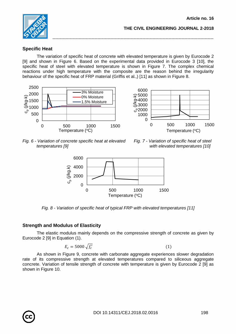
Article no. 16


---------------------------------------------------------------------------------------------------------------

DOI 10.14311/CEJ.2018.02.0016 198

Specific Heat

The variation of specific heat of concrete with elevated temperature is given by Eurocode 2 [9] and shown in Figure 6. Based on the experimental data provided in Eurocode 3 [10], the specific heat of steel with elevated temperature is shown in Figure 7. The complex chemical reactions under high temperature with the composite are the reason behind the irregularity behaviour of the specific heat of FRP material (Griffis et al.,) [11] as shown in Figure 8.

Fig. 6 - Variation of concrete specific heat at elevated temperatures [9]

Fig. 7 - Variation of specific heat of steel with elevated temperatures [10]

Fig. 8 - Variation of specific heat of typical FRP with elevated temperatures [11]

Strength and Modulus of Elasticity

The elastic modulus mainly depends on the compressive strength of concrete as given by Eurocode 2 [9] in Equation (1).

𝐸𝑐 = 5000 √𝑓𝑐′ (1)

As shown in Figure 9, concrete with carbonate aggregate experiences slower degradation rate of its compressive strength at elevated temperatures compared to siliceous aggregate concrete. Variation of tensile strength of concrete with temperature is given by Eurocode 2 [9] as shown in Figure 10.

0

500

1000

1500

2000

2500

0 500 1000 1500

cp

(j/k

g-k

)

Temperature (oC)

3% Moisture

0% Moisture

1.5% Moisture

0100020003000400050006000

0 500 1000 1500

cp

(j/k

g-k

)Temperature (oC)

0

2000

4000

6000

0 500 1000 1500

cp

(j/k

g.k

)

Temperature (oC)

Article no. 16


---------------------------------------------------------------------------------------------------------------

DOI 10.14311/CEJ.2018.02.0016 199

Fig. 9 - Variation of compressive strength of concrete with temperature [9]

Fig. 10 - Reduction of concrete tensile strength with elevated temperatures [9]

As shown in Figure 11, steel loses more than 50% of its original strength at about 600°C [10]. Likewise, it is clear from Figure 12 that, the modulus of elasticity of the reinforcement steel decreases with elevated temperature.

Fig. 11 - Reduction of yield strength of steel with elevated temperatures [10]

Fig. 12 - Reduction in modulus of elasticity of steel with elevated temperatures [10]

Figure 13 shows the reduction in strength of CFRP and GFRP with elevated temperature. Likewise, stiffness of FRP materials also has similar rapid degradation with elevated temperature as shown in Figure 14.

Fig. 13 - Reduction in strength for various FRP materials with elevated temperatures [4]

Fig.14 - Reduction of stiffness of CFRP with elevated temperatures [12]

0

0,5

1

1,5

-300 200 700 1200

f C,t/f

CK

Temperature (oC)

CalcareousAggregateSiliceousAggregate

0

0,5

1

1,5

0 200 400 600 800 100012001400

Re

du

ction

in

te

nsile

str

eng

th

Temperature (oC)

0

0,2

0,4

0,6

0,8

1

1,2

0 500 1000 1500

Re

du

ction

in

fy

Temperature (oC)

0

50000

100000

150000

200000

250000

0 500 1000 1500

Es (

MP

a)

Temperature (oC)

0

20

40

60

80

100

120

0 100 200 300 400 500 600 700 800

% o

f in

itia

l str

en

gth

Temperature (oC)

Carbon/Epoxy FRP

Glass or Aramid/Epoxy FRP

0

0,2

0,4

0,6

0,8

1

1,2

0 500 1000

E /

Eo

Temperature (oC)

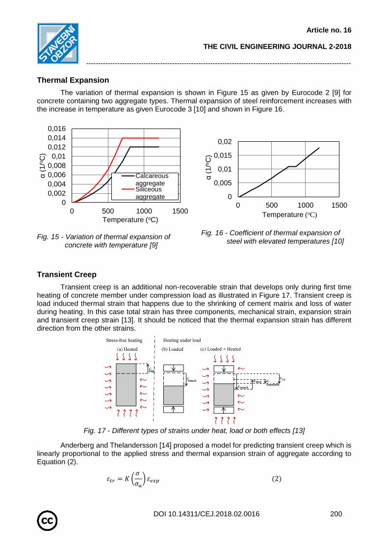
Article no. 16


---------------------------------------------------------------------------------------------------------------

DOI 10.14311/CEJ.2018.02.0016 200

Thermal Expansion

The variation of thermal expansion is shown in Figure 15 as given by Eurocode 2 [9] for concrete containing two aggregate types. Thermal expansion of steel reinforcement increases with the increase in temperature as given Eurocode 3 [10] and shown in Figure 16.

Fig. 15 - Variation of thermal expansion of concrete with temperature [9]

Fig. 16 - Coefficient of thermal expansion of steel with elevated temperatures [10]

Transient Creep

Transient creep is an additional non-recoverable strain that develops only during first time heating of concrete member under compression load as illustrated in Figure 17. Transient creep is load induced thermal strain that happens due to the shrinking of cement matrix and loss of water during heating. In this case total strain has three components, mechanical strain, expansion strain and transient creep strain [13]. It should be noticed that the thermal expansion strain has different direction from the other strains.

Fig. 17 - Different types of strains under heat, load or both effects [13]

Anderberg and Thelandersson [14] proposed a model for predicting transient creep which is linearly proportional to the applied stress and thermal expansion strain of aggregate according to Equation (2).

𝜀𝑡𝑟 = 𝐾 (𝜎

𝜎𝑢) 𝜀𝑒𝑥𝑝 (2)

0

0,002

0,004

0,006

0,008

0,01

0,012

0,014

0,016

0 500 1000 1500

α (

1/o

C)

Temperature (oC)

CalcareousaggregateSiliceousaggregate 0

0,005

0,01

0,015

0,02

0 500 1000 1500α

(1/o

C)

Temperature (oC)

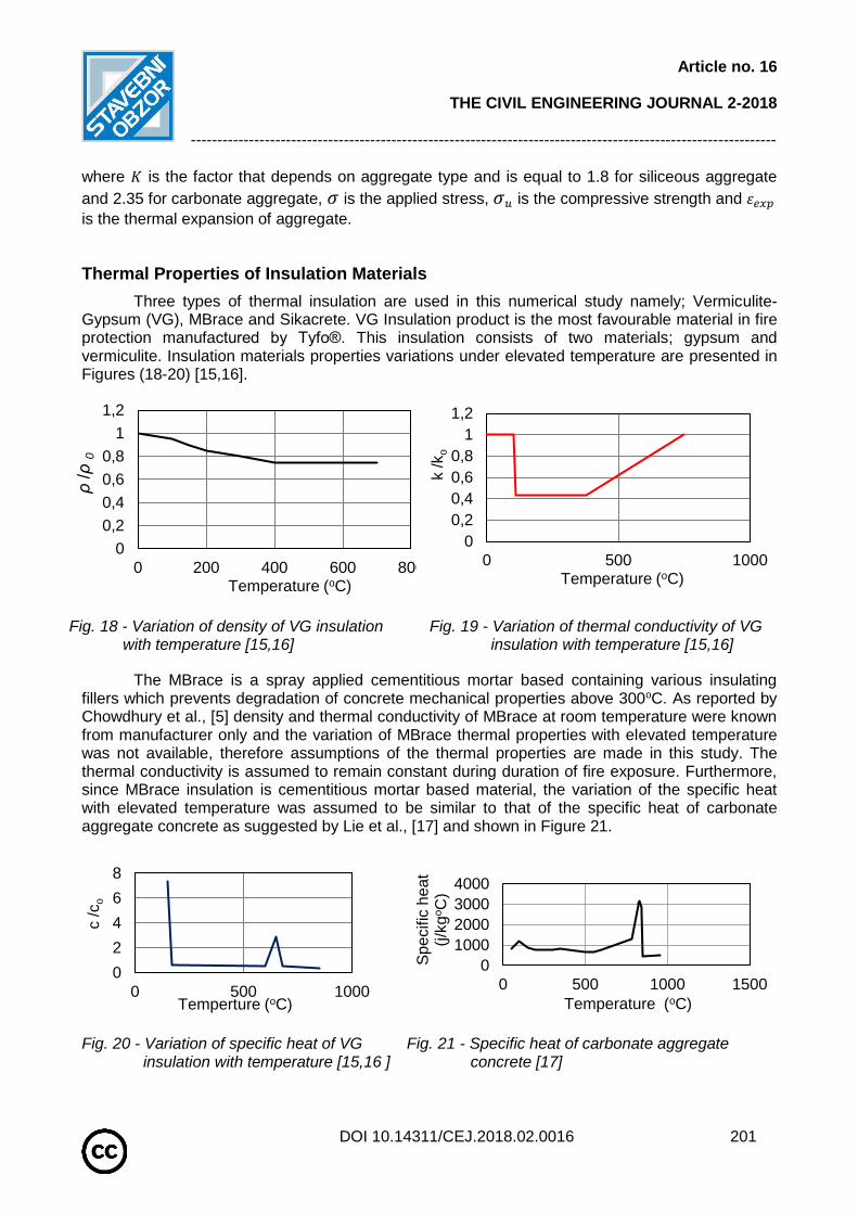
Article no. 16


---------------------------------------------------------------------------------------------------------------

DOI 10.14311/CEJ.2018.02.0016 201

where 𝐾 is the factor that depends on aggregate type and is equal to 1.8 for siliceous aggregate

and 2.35 for carbonate aggregate, 𝜎 is the applied stress, 𝜎𝑢 is the compressive strength and 𝜀𝑒𝑥𝑝

is the thermal expansion of aggregate.

Thermal Properties of Insulation Materials

Three types of thermal insulation are used in this numerical study namely; Vermiculite-Gypsum (VG), MBrace and Sikacrete. VG Insulation product is the most favourable material in fire protection manufactured by Tyfo®. This insulation consists of two materials; gypsum and vermiculite. Insulation materials properties variations under elevated temperature are presented in Figures (18-20) [15,16].

Fig. 18 - Variation of density of VG insulation with temperature [15,16]

Fig. 19 - Variation of thermal conductivity of VG insulation with temperature [15,16]

The MBrace is a spray applied cementitious mortar based containing various insulating fillers which prevents degradation of concrete mechanical properties above 300oC. As reported by Chowdhury et al., [5] density and thermal conductivity of MBrace at room temperature were known from manufacturer only and the variation of MBrace thermal properties with elevated temperature was not available, therefore assumptions of the thermal properties are made in this study. The thermal conductivity is assumed to remain constant during duration of fire exposure. Furthermore, since MBrace insulation is cementitious mortar based material, the variation of the specific heat with elevated temperature was assumed to be similar to that of the specific heat of carbonate aggregate concrete as suggested by Lie et al., [17] and shown in Figure 21.

Fig. 20 - Variation of specific heat of VG insulation with temperature [15,16 ]

Fig. 21 - Specific heat of carbonate aggregate concrete [17]

0

0,2

0,4

0,6

0,8

1

1,2

0 200 400 600 800

ρ/ρ

0

Temperature (oC)

0

0,2

0,4

0,6

0,8

1

1,2

0 500 1000

k /k

o

Temperature (oC)

0

2

4

6

8

0 500 1000

c /c

o

Temperture (oC)

0

1000

2000

3000

4000

0 500 1000 1500

Sp

ecific

hea

t

(j/k

goC

)

Temperature (oC)

Article no. 16


---------------------------------------------------------------------------------------------------------------

DOI 10.14311/CEJ.2018.02.0016 202

The Sikacrete®-213F is a spray applied mortar based protection system with vermiculite and acts as the insulating filler, which gives strong thermal insulation properties. As reported by Masoud et al., [18] the density of Sikacrete is equal to 700 Kg/m3 and the variations in thermal conductivity and specific heat are given by Eqs. (3) and (4), respectively.

𝐾𝑐(𝑇) = 0.46 (𝑇

1000)

2

− 0.21 (𝑇

1000) + 0.32 𝑖𝑛 (

𝑊

𝑚. 𝐾) (3)

𝐶𝑐(𝑇) = 14.96 (𝑇

100)

2

− 116.4 (𝑇

100) + 1611 𝑖𝑛 (

𝐽

𝐾𝑔. 𝐾) (4)

MODELLING AND NONLINEAR SOLUTION METHODOLOGY

The general approach for performing the thermal and structural modelling and nonlinear analysis are summarized in Figure 22, the main steps include:

1. Building 3-D nonlinear numerical model of the RC column. This process includes member geometry, appropriate definitions for the materials of concrete, reinforcement steel, FRP and boundary conditions. Two separates finite element models were created, one for thermal analysis and the other for structural analysis.

2. Appling the thermal loads in the form of transient temperatures versus time to the outer surface of column by utilizing regime function method in ANSYS. The thermal load is applied according the ASTM E119 [7].

3. After comparing and verification of the predicted with measured temperatures in the cross section of the column, the temperature data is used in the load step information of the structural model.

4. Applying service load and the predicted thermal loads into the structural model through two cumulative load steps. In case of earlier non-convergence problem has occurred, kill and birth technique is used to exclude the crushed elements from matrix and continue the solution.

5. If the column did not fail after 5 hours of fire exposure, the service load will be increased gradually through regime function method in ANSYS to induce failure.

6. Evaluate the vertical displacement of the column during the fire exposure time to the fire and comparing it with experimental measured ones.

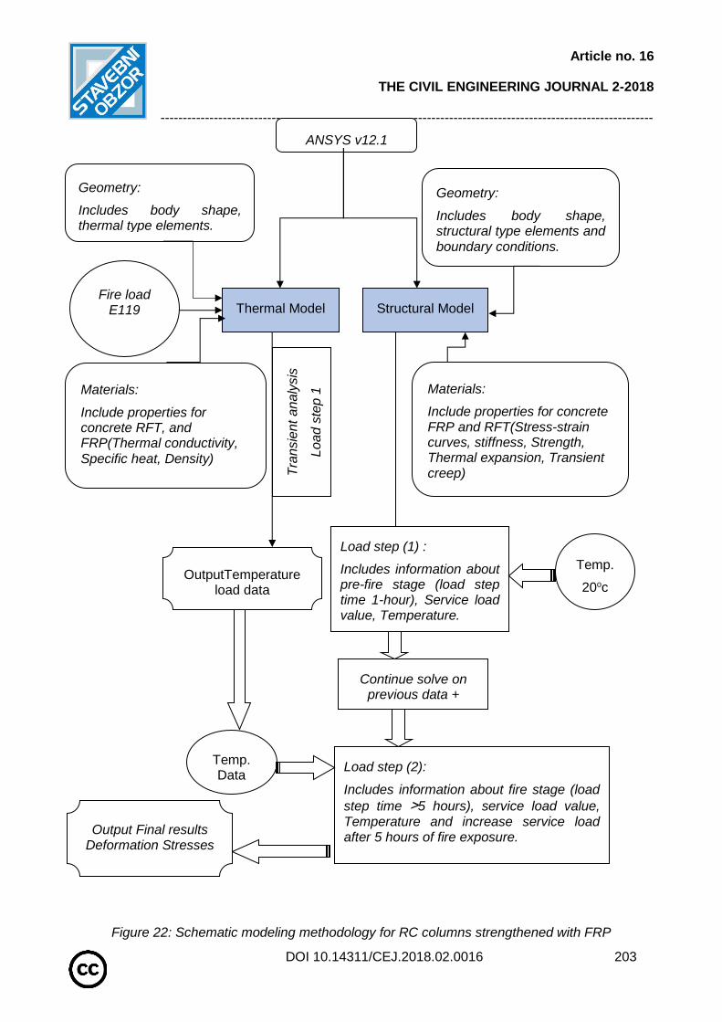
Article no. 16


---------------------------------------------------------------------------------------------------------------

DOI 10.14311/CEJ.2018.02.0016 203

Figure 22: Schematic modeling methodology for RC columns strengthened with FRP

Fire load E119

ANSYS v12.1

Thermal Model Structural Model

Geometry:

Includes body shape, thermal type elements.

Materials:

Include properties for concrete RFT, and FRP(Thermal conductivity,

Specific heat, Density)

OutputTemperature load data

Tra

nsie

nt

ana

lysis

Loa

d s

tep 1

Geometry:

Includes body shape, structural type elements and boundary conditions.

Materials:

Include properties for concrete FRP and RFT(Stress-strain curves, stiffness, Strength, Thermal expansion, Transient creep)

Load step (1) :

Includes information about pre-fire stage (load step time 1-hour), Service load value, Temperature.

Temp.

20oc

Continue solve on previous data +

Load step (2):

Includes information about fire stage (load

step time <5 hours), service load value, Temperature and increase service load after 5 hours of fire exposure.

Temp.Data

Output Final results Deformation Stresses

Article no. 16


---------------------------------------------------------------------------------------------------------------

DOI 10.14311/CEJ.2018.02.0016 204

NUMERICAL VERIFICATION STUDY

A numerical study was conducted for verification of the proposed model for FRP strengthened RC columns subjected to elevated temperatures due to fire. Four studied experimental cases by other researchers are chosen for the verification. Table (1) gives a summary of these cases. The first two columns were tested by Bisby [4], the third column was tested by Chowdhury et al., [5], while the last column was tested by Cree et al., [6].

Tab. 1 - Summary of the case studies data

Case study

Diameter (mm)

Length (mm)

Longitudinal steel bars

Transverse steel bars

f'c (MPa)

FRP wrap

Insulation (mm)

Service load (KN)

1 400 3810 8T20 11.3 mm spiral

at 50 mm pitch 40

1-layer CFRP

32-VG 2515

2 400 3810 8T20 11.3 mm spiral

at 50 mm pitch 39

1-layer CFRP

57-VG 2515

3 400 3810 8T20 11.3 mm spiral

at 50 mm pitch 32.9

2-layers CFRP

53-MBrace

2635

4 400 3810 8T20 10 mm spiral at

50 mm pitch 38.5

2-layers CFRP

44-Sikacrete

3054

Element Types for Representation

The element types used to represent the different materials for all columns are given in Table 2. Each type of analysis required specific types of elements in order to get a realistic solution.

Tab. 2 - Element types used for thermal and structural analyses

Material Thermal analysis Structural analysis

Concrete SOLID70 SOLID65

Steel bars LINK33 LINK8

CFRP layer SHELL57 SHELL41

Insulation SOLID70 SOLID45

Description and Geometry

All columns were experimentally tested in the National Research Council in Canada (NRC) using special furnace which is capable of applying elevated temperature according to standard fire test ASTM E119 [7] and service load via hydraulic jack. All columns have circular section with concrete cover of 40 mm and wrapped with CFRP sheets along their full length. The sections of the columns are symmetric about x and z axes therefore, only quarter of the section was modelled in ANSYS, the finite element meshing is shown in Figure 23.

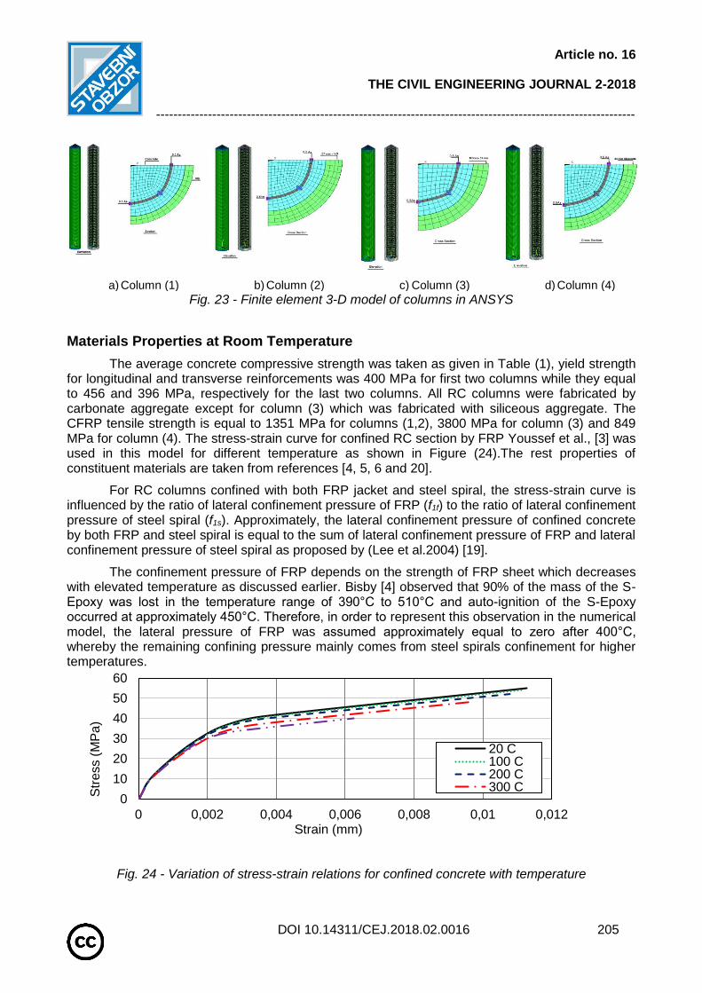
Article no. 16


---------------------------------------------------------------------------------------------------------------

DOI 10.14311/CEJ.2018.02.0016 205

a) Column (1) b) Column (2) c) Column (3) d) Column (4)

Fig. 23 - Finite element 3-D model of columns in ANSYS

Materials Properties at Room Temperature

The average concrete compressive strength was taken as given in Table (1), yield strength for longitudinal and transverse reinforcements was 400 MPa for first two columns while they equal to 456 and 396 MPa, respectively for the last two columns. All RC columns were fabricated by carbonate aggregate except for column (3) which was fabricated with siliceous aggregate. The CFRP tensile strength is equal to 1351 MPa for columns (1,2), 3800 MPa for column (3) and 849 MPa for column (4). The stress-strain curve for confined RC section by FRP Youssef et al., [3] was used in this model for different temperature as shown in Figure (24).The rest properties of constituent materials are taken from references [4, 5, 6 and 20].

For RC columns confined with both FRP jacket and steel spiral, the stress-strain curve is influenced by the ratio of lateral confinement pressure of FRP (f1f) to the ratio of lateral confinement pressure of steel spiral (f1s). Approximately, the lateral confinement pressure of confined concrete by both FRP and steel spiral is equal to the sum of lateral confinement pressure of FRP and lateral confinement pressure of steel spiral as proposed by (Lee et al.2004) [19].

The confinement pressure of FRP depends on the strength of FRP sheet which decreases with elevated temperature as discussed earlier. Bisby [4] observed that 90% of the mass of the S-Epoxy was lost in the temperature range of 390°C to 510°C and auto-ignition of the S-Epoxy occurred at approximately 450°C. Therefore, in order to represent this observation in the numerical model, the lateral pressure of FRP was assumed approximately equal to zero after 400°C, whereby the remaining confining pressure mainly comes from steel spirals confinement for higher temperatures.

Fig. 24 - Variation of stress-strain relations for confined concrete with temperature

0

10

20

30

40

50

60

0 0,002 0,004 0,006 0,008 0,01 0,012

Str

ess (

MP

a)

Strain (mm)

20 C100 C200 C300 C

Article no. 16


---------------------------------------------------------------------------------------------------------------

DOI 10.14311/CEJ.2018.02.0016 206

THERMAL NUMERICAL RESULTS

Figure 25 shows the temperature distribution through the section of column (1) after one, two, three and five hours of exposure. Furthermore, the obtained thermal results using the present model as well as the experimental results obtained by other researchers for the four columns are shown in Figures. 26-29.

For column (1) in Figure 26, the temperature between FRP and concrete changes from room temperature up to 425°C experimentally and 440°C numerically with 3.5% variance after five hours, however, the overall average variance is approximately 24%. As for RFT, temperature increases up to 200°C experimentally and 237°C numerically with 19% variance after five hours, however, the overall average variance is 14%. As for concrete, temperature increases up to 165°C experimentally and 124°C numerically with 25% variance after five hours, however, the overall average variance is 17%. For column (2) in Figure 27, the temperature between FRP and concrete changes from room temperature up to 180°C experimentally and 258°C numerically with 43% variance after five hours, however, the overall average variance exceeds 50%. This happened because the temperature of FRP from first hour to fourth hour remained unchanged below 100°C regardless the continuous heat transfer. As for RFT, temperature increases up to 104°C experimentally and 130°C numerically with 25% variance after five hours, however, the overall average variance is 20%. As for concrete, temperature increases up to 92°C experimentally and 95°C numerically with 3.3% variance after five hours, however, the overall variance is 12%. For column (3) in Figure 28, the temperature between FRP and concrete changes from room temperature up to 480°C experimentally and 460°C numerically with 4% variance after five hours, however, the overall average variance is 12%. As for RFT, temperature increases up to 280°C experimentally and 276°C numerically with 2% variance after five hours, however, the overall average variance is approximately 15%. As for concrete, temperature increases up to 200°C experimentally and 185°C numerically with 8% variance after five hours, however, the overall variance is 27%. For column (4) in Figure 29, the temperature between FRP and concrete changes from room temperature up to 420°C experimentally and 440°C numerically with 5% variance after four hours, however, the overall average variance is 9%. As for concrete, temperature increases up to 180°C experimentally and 220°C numerically with 23% variance after four hours, however, the overall variance is 17%. In general, it can be concluded that the numerically predicted results are in good agreement with experimental ones. The main reason for the variances in prediction temperature mentioned above is generally due to information lack of actual initial values or actual variation with temperature for thermal conductivity, specific heat and density of the used materials in the conducted experiments. These data are not always available from researchers or manufacturers, therefore, standard curves for thermal properties which are discussed in literature have been used in this analysis.

a) After one hour b) After two hours c) After three hours d) After five hours

Fig. 25 - Column (1): Numerically predicted temperature distribution in the column cross-section

Article no. 16


---------------------------------------------------------------------------------------------------------------

DOI 10.14311/CEJ.2018.02.0016 207

Fig. 26 - Column (1): Numerical thermal results compared to published results




0

100

200

300

400

500

0 60 120 180 240 300

Te

mp

era

ture

(o

C)

Time (minutes)

Concrete 100mm Numerical [This Work]

RFT Numerical [This Work]

FRP/Concrete Numerical [This Work]

Concrete 100mm Experimental (Bisby, 2003)

RFT Experimental (Bisby, 2003)

FRP/Concrete Experimental (Bisby, 2003)

0

50

100

150

200

250

300

0 60 120 180 240 300

Tem

pera

ture

(o

C)

Time (minutes)




Concrete 100mm Experimental (Bisby, 2003)

RFT Experimental (Bisby, 2003)

FRP/Concrete Experimental (Bisby, 2003)

0

100

200

300

400

500

600

0 60 120 180 240 300

Te

mp

era

ture

(o

C)

Time (minutes)




Concrete 100mm Experimental (Chowdhury et al,2007)RFT Experimental (Chowdhury et al, 2007)

0

100

200

300

400

500

0 60 120 180 240

Te

mp

era

ture

(o

C)

Time (minutes)

Concrete 50mm [This Work]

FRP Surface [This Work]

Concrete 50mm Experimental (Cree et al,2012)

FRP Surface Experimental (Cree et al,2012)

Article no. 16


---------------------------------------------------------------------------------------------------------------

DOI 10.14311/CEJ.2018.02.0016 208

STRUCTURAL NUMERICAL RESULTS

The obtained structural results for the numerically predicted axial deformation under applied service load and fire exposure for specific time are plotted in Figures 30-33 for the four studied columns, and results are compared to the axial deformation measured in published experimental works. From these figures, it can be observed that the numerically predicted results are in good agreement with experimental ones. For column (1) shown in Figure 30, the main deformation is small elongation till first two hours, then elongation strain decreases due to increase of transient creep strain with elevated temperature which may acts against elongation strain until crushing of column. Elongation strain has more influence than transient creep strain in column (2) shown in Figure 31 due to lower exposed of temperature comparing with column (1). As for columns (3,4) shown in Figures 32, 33, columns experienced elongation strain in first two hours then transient creep strain starts to influence the overall deformations.

Fig. 30 - Column (1): Axial deformation of the column during fire exposure




-15

-13

-11

-9

-7

-5

-3

-1

1

3

0 60 120 180 240 300

Axia

l d

efo

rma

tion

(m

m)

Exposure time (minutes)

Numerical [ThisWork]Experimental(Bisby, 2003)

-15

-13

-11

-9

-7

-5

-3

-1

1

0 60 120 180 240 300

Axia

l d

efo

rma

tion

s (

mm

)


Numerical [ThisWork]

Experimental(Bisby, 2003)

-15

-13

-11

-9

-7

-5

-3

-1

1

0 60 120 180 240 300

Axia

l d

efo

rma

tion

(m

m)


Numerical [This Work]

Experimental(Chowdhury et al, 2007)

-20-18-16-14-12-10-8-6-4-202

0 60 120 180 240 300

Axia

l d

efo

rma

tion

(m

m)


Numerical [This Work]

Eperimental (Cree et al,2012)

Article no. 16


---------------------------------------------------------------------------------------------------------------

DOI 10.14311/CEJ.2018.02.0016 209

Table 3 summarizes the numerically predicted and experimental results and provides the ultimate capacity of the columns at normal temperature 20°C.

Tab. 3 - Summary of experimental and numerically predicted results

Case study

Fire resistance (min)

Failure load (KN)

Variance in failure

load

Predicted capacity at ambient

temperature (KN) Experimental Numerical Experimental Numerical

1 <300 <300 4473 5018 1.12 5800

2 <300 <300 4680 5393 1.15 5800

3 <300 <300 4583 4682 1.02 5600

4 <240 <240 4980 5647 1.13 6600

CONCLUSIONS

The paper presents numerical modelling procedure by finite elements that simulate the performance of RC column strengthened with CFRP sheets and thermally insulated when exposed to standard fire test under service loads. Numerical modelling and nonlinear analysis are performed using the general purpose software ANSYS 12.1. The proposed procedure is verified by comparing the numerical results with experimental results available in the published literature. Based on the obtained numerical results, the following conclusions can be drawn.

1. The numerically predicted results of the proposed model are in good agreement with published experimental results for both thermal and structural aspects. The accuracy of thermal prediction for FRP, RFT and concrete are 78%, 84% and 82%, respectively. Also, for structural failure load prediction, the accuracy is 89%.

2. The proposed model can accurately predict thermal and structural response for different configurations regarding constituent material properties or insulation type and thickness.

3. The proposed model provides a reasonable accurate axial deformation response due to consideration of transient creep strain in the analysis.

4. The axial deformation response for column under fire tend to expand in early stage of fire exposure followed by contraction due to degradation in stiffness and presence of transient creep strain which acts against expansion strain of burned RC column.

5. The proposed model provides an economic tool for check and design of fire insulation layers for FRP strengthened RC columns. It should be noticed that, the modelling needs to be verified against experimental works.

REFERENCES

1. ANSYS–Release Version 12.1.0, “A Finite Element Computer Software and User Manual for

Nonlinear Structural Analysis”, ANSYS Inc. Canonsburg, PA., (2009). 2. Chowdhury,E.U., “Behavior of Fiber Reinforced Polymer Confined Reinforced Concrete Columns

Under Fire Condition.”, PhD thesis, Dept. of Civil Engineering Queen’s Univ., Kingston, Ont., Canada, (2009).

3. Youssef, M. N., Feng, M. Q.and Mosallam, A. S., “Stress-Strain Model for Concrete Confined by FRP Composites”, Composites Part B, V. 38, pp. 614-628, (2007).

4. Bisby, L. A., “Fire Behavior of FRP Reinforced or Confined Concrete.”, PhD thesis, Dept. of Civil Engineering Queen’s Univ., Kingston, Ont., Canada, (2003).

5. Chowdhury,E.U., Bisby, L.A. and Green, M.F., "Investigation of Insulated FRP-Wrapped Reinforced Concrete Columns in Fire”, Fire Safety Journal, 42 (2007),pp. 452–460.

Article no. 16


---------------------------------------------------------------------------------------------------------------

DOI 10.14311/CEJ.2018.02.0016 210

6. Cree, C., Chowdhury,E.U., Bisby, L.A., Green, M.F., and Benichou, N., “Performance in Fire of FRP-Strengthened and Insulated Reinforced Concrete Columns”, Fire Safety Journal, 54 (2012), pp. 86–95.

7. ASTM, "Standard Test Methods for Fire Tests of Building Construction and Materials", ASTM Standard E119, American Society for Testing of Materials, West Conshohocken, PA, (2002).

8. Bisby, L.A., Green, M.F.and Kodur, V.K.R., “Modeling the Behavior of Fiber Reinforced Polymer-Confined Concrete Columns Exposed to Fire”, 10.1061/(ASCE)1090-0268(2005)9:1(15).

9. Eurocode2, “Design of Concrete Structures, ENV EC2 Part 1.2",Eurocode, (2004). 10. Eurocode 3, “Design of Steel Structures, ENV EC3 Part 1.2.",Eurocode, (2005). 11. Griffis, C., Masmura, R. and Chang, C., "Thermal Response of Graphite Epoxy Composite Subjected

to Rapid Heating", Environmental Effects on Composite Materials, Vol. 2, pp. 245- 260, (1984). 12. Williams, B, Kodur,V, Green, M. and Bisby, L., "Fire Endurance of Fiber-Reinforced Polymer

Strengthened Concrete T-Beams,", J ACI Structural, vol. 105, No. 1, pp. 60-67, (2008). 13. Torelli, G., Mandal, P., Gillie, M. and ,Tran, V.X., "Concrete Strains under Transient Thermal

Conditions: A State-of-The-Art Review", Engineering Structures 127, pp. 172–188, (2016). 14. Anderberg, Y. and Thelandersson, S., “Stress and Deformation Characteristics of Concrete at High

Temperature: 2. Experimental Investigation and Material Behavior Model”, Bull. No. 46, Lund,(1976). 15. Park, S. H., Manzello, S., L., Bentz, D., P., and Mizukami, T., “Determining Thermal Properties of

Gypsum Board at ElevatedTemperatures”, Fire and Materials, (2009), pp. 237-250. 16. Cramer, S.M., Friday, O.M., White, R.H., and Sriprutkiat, G., “Mechanical Properties of Gypsum

Board at Elevated Temperatures”, Fire and Materials (2003) 33–42. 17. Lie, T. T., and Kodur, V. K. R., "Thermal Properties of Fibre Reinforced Concrete at Elevated

Temperatures", National Research Council Canada, Institute for Research in Construction), 04-01, (1995).

18. Masoud, A.Z., “Structural and Thermal Behaviour of Insulated FRP Strengthened Reinforced Concrete Beams and Slabs in Fire”, PhD Thesis, Dept. of Civil Engineering Queen’s Univ., Kingston, Ont., Canada, (2013).

19. Lee, J.Y., Oh, Y.J., Park, J., S.and Mansour, M.Y., "Behavior of Concrete Columns Confined with Both Spiral and Fiber Composites", 13th World Conference on Earthquake Engineering, No. 3051, (2004).

20. Hawileh, R., A., Naser, M., Zaidan, W., and Rasheed, H. A., “Modeling of Insulated CFRPStrengthened Reinforced Concrete T-beam Exposed to Fire”, Engineering Structures, 31( 12) (2009), pp. 3072–3079.

Article no. 17


-----------------------------------------------------------------------------------------------------------------

DOI 10.14311/CEJ.2018.02.0017 211

DISCRETE ELEMENT MODELING OF STRENGTH PROPERTIES AND FAILURE MODES OF QH-E LUNAR SOIL SIMULANT AT

LOW CONFINING STRESSES

Li Yun-Li 1, Zou Wei-Lie1,2*, Wu Wen-Ping1 and Chen Lun3

1. Key Laboratory of Geotechnical and Structural Engineering Safety of Hubei Province, School of Civil Engineering, Wuhan University, Wuhan 430072, China; liyunli @whu.edu.cn

2. School of Civil Engineering, Xijing University, Xi’an 710123, China; [email protected]

3. State Key Laboratory of Hydroscience and Engineering, Tsinghua University, Beijing 100084, China; [email protected]

ABSTRACT

In this paper, discrete element method (DEM) is used to investigate the strength properties and failure modes of QH-E lunar soil simulant at the low confining stress. The deviator stress-axial strain curves and volumetric strain-axial strain curves are obtained based on DEM simulations, which are basically consistent with the experimental results at the low confining stresses, and the lower confining stress is, the closer to the experimental curves will obtain. Moreover, for a given low confining stress, the effects of porosity and friction coefficient on strength properties of QH-E samples are discussed. The results show that the peak stress, residual stress and axial strain corresponding to the peak stress obviously decrease with the increase of the porosity, while slightly increase with the increase of the friction coefficient. Furthermore, the whole failure processes and failure modes at different low confining stresses are also observed by DEM simulations. The simulated results indicate that the V-type shear zone (double shear bands) is the main failure mode at the low confining stress, and then the V-type shear zone gradually changes to a single shear band (along the horizontal direction about 52o) with the increase of the confining stress.

KEYWORDS Discrete element method, Triaxial compression test, Mechanical properties, Failure modes

INTRODUCTION

Manned lunar exploration has attracted renewed interest, many countries are preparing their own plans for lunar exploration [1]. The lunar soil will be the first lunar material that explorers and exploration equipment directly contact when they land on the Moon and its mechanical characteristics are important to lunar exploration. Because of the limited amount of lunar regolith brought back to Earth by the Apollo missions, lunar soil simulants, as the substitutions of real lunar soils, was developed to investigate the mechanical properties of real lunar soils [2-6], as well as the interaction behaviour between exploration equipment and lunar soils.

Particle flow code (PFC) numerical simulation as a discrete element method (DEM) is being constantly used in the research of the basic physical and mechanical properties of granular materials. The lunar soil consists of discrete solid particles, which can be classified as a granular material or similar to granular soil [2]. Many researchers investigated the mechanical properties of the lunar soil stimulants using PFC numerical simulation. For example, Hasan and Alshibli [1]

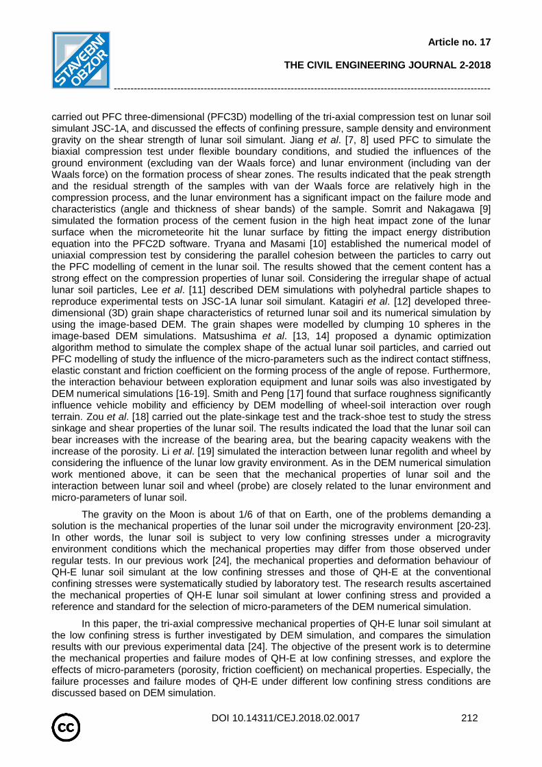
Article no. 17


-----------------------------------------------------------------------------------------------------------------

DOI 10.14311/CEJ.2018.02.0017 212

carried out PFC three-dimensional (PFC3D) modelling of the tri-axial compression test on lunar soil simulant JSC-1A, and discussed the effects of confining pressure, sample density and environment gravity on the shear strength of lunar soil simulant. Jiang et al. [7, 8] used PFC to simulate the biaxial compression test under flexible boundary conditions, and studied the influences of the ground environment (excluding van der Waals force) and lunar environment (including van der Waals force) on the formation process of shear zones. The results indicated that the peak strength and the residual strength of the samples with van der Waals force are relatively high in the compression process, and the lunar environment has a significant impact on the failure mode and characteristics (angle and thickness of shear bands) of the sample. Somrit and Nakagawa [9] simulated the formation process of the cement fusion in the high heat impact zone of the lunar surface when the micrometeorite hit the lunar surface by fitting the impact energy distribution equation into the PFC2D software. Tryana and Masami [10] established the numerical model of uniaxial compression test by considering the parallel cohesion between the particles to carry out the PFC modelling of cement in the lunar soil. The results showed that the cement content has a strong effect on the compression properties of lunar soil. Considering the irregular shape of actual lunar soil particles, Lee et al. [11] described DEM simulations with polyhedral particle shapes to reproduce experimental tests on JSC-1A lunar soil simulant. Katagiri et al. [12] developed three-dimensional (3D) grain shape characteristics of returned lunar soil and its numerical simulation by using the image-based DEM. The grain shapes were modelled by clumping 10 spheres in the image-based DEM simulations. Matsushima et al. [13, 14] proposed a dynamic optimization algorithm method to simulate the complex shape of the actual lunar soil particles, and carried out PFC modelling of study the influence of the micro-parameters such as the indirect contact stiffness, elastic constant and friction coefficient on the forming process of the angle of repose. Furthermore, the interaction behaviour between exploration equipment and lunar soils was also investigated by DEM numerical simulations [16-19]. Smith and Peng [17] found that surface roughness significantly influence vehicle mobility and efficiency by DEM modelling of wheel-soil interaction over rough terrain. Zou et al. [18] carried out the plate-sinkage test and the track-shoe test to study the stress sinkage and shear properties of the lunar soil. The results indicated the load that the lunar soil can bear increases with the increase of the bearing area, but the bearing capacity weakens with the increase of the porosity. Li et al. [19] simulated the interaction between lunar regolith and wheel by considering the influence of the lunar low gravity environment. As in the DEM numerical simulation work mentioned above, it can be seen that the mechanical properties of lunar soil and the interaction between lunar soil and wheel (probe) are closely related to the lunar environment and micro-parameters of lunar soil.

The gravity on the Moon is about 1/6 of that on Earth, one of the problems demanding a solution is the mechanical properties of the lunar soil under the microgravity environment [20-23]. In other words, the lunar soil is subject to very low confining stresses under a microgravity environment conditions which the mechanical properties may differ from those observed under regular tests. In our previous work [24], the mechanical properties and deformation behaviour of QH-E lunar soil simulant at the low confining stresses and those of QH-E at the conventional confining stresses were systematically studied by laboratory test. The research results ascertained the mechanical properties of QH-E lunar soil simulant at lower confining stress and provided a reference and standard for the selection of micro-parameters of the DEM numerical simulation.

In this paper, the tri-axial compressive mechanical properties of QH-E lunar soil simulant at the low confining stress is further investigated by DEM simulation, and compares the simulation results with our previous experimental data [24]. The objective of the present work is to determine the mechanical properties and failure modes of QH-E at low confining stresses, and explore the effects of micro-parameters (porosity, friction coefficient) on mechanical properties. Especially, the failure processes and failure modes of QH-E under different low confining stress conditions are discussed based on DEM simulation.

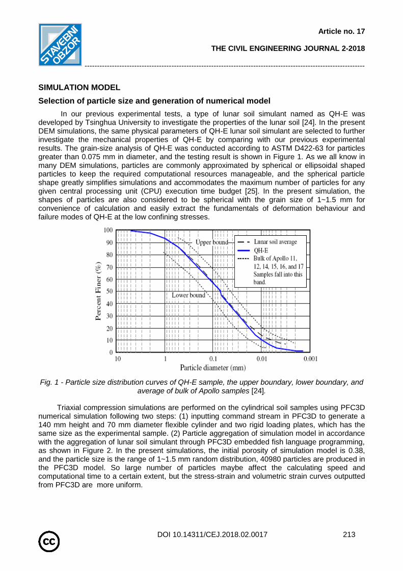
Article no. 17


-----------------------------------------------------------------------------------------------------------------

DOI 10.14311/CEJ.2018.02.0017 213

SIMULATION MODEL

Selection of particle size and generation of numerical model

In our previous experimental tests, a type of lunar soil simulant named as QH-E was developed by Tsinghua University to investigate the properties of the lunar soil [24]. In the present DEM simulations, the same physical parameters of QH-E lunar soil simulant are selected to further investigate the mechanical properties of QH-E by comparing with our previous experimental results. The grain-size analysis of QH-E was conducted according to ASTM D422-63 for particles greater than 0.075 mm in diameter, and the testing result is shown in Figure 1. As we all know in many DEM simulations, particles are commonly approximated by spherical or ellipsoidal shaped particles to keep the required computational resources manageable, and the spherical particle shape greatly simplifies simulations and accommodates the maximum number of particles for any given central processing unit (CPU) execution time budget [25]. In the present simulation, the shapes of particles are also considered to be spherical with the grain size of 1~1.5 mm for convenience of calculation and easily extract the fundamentals of deformation behaviour and failure modes of QH-E at the low confining stresses.

Fig. 1 - Particle size distribution curves of QH-E sample, the upper boundary, lower boundary, and average of bulk of Apollo samples [24].

Triaxial compression simulations are performed on the cylindrical soil samples using PFC3D numerical simulation following two steps: (1) inputting command stream in PFC3D to generate a 140 mm height and 70 mm diameter flexible cylinder and two rigid loading plates, which has the same size as the experimental sample. (2) Particle aggregation of simulation model in accordance with the aggregation of lunar soil simulant through PFC3D embedded fish language programming, as shown in Figure 2. In the present simulations, the initial porosity of simulation model is 0.38, and the particle size is the range of 1~1.5 mm random distribution, 40980 particles are produced in the PFC3D model. So large number of particles maybe affect the calculating speed and computational time to a certain extent, but the stress-strain and volumetric strain curves outputted from PFC3D are more uniform.

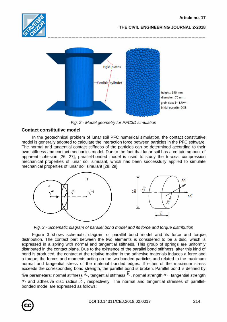
Article no. 17


-----------------------------------------------------------------------------------------------------------------

DOI 10.14311/CEJ.2018.02.0017 214

Fig. 2 - Model geometry for PFC3D simulation

Contact constitutive model

In the geotechnical problem of lunar soil PFC numerical simulation, the contact constitutive model is generally adopted to calculate the interaction force between particles in the PFC software. The normal and tangential contact stiffness of the particles can be determined according to their own stiffness and contact mechanics model. Due to the fact that lunar soil has a certain amount of apparent cohesion [26, 27], parallel-bonded model is used to study the tri-axial compression mechanical properties of lunar soil simulant, which has been successfully applied to simulate mechanical properties of lunar soil simulant [28, 29].

Fig. 3 - Schematic diagram of parallel bond model and its force and torque distribution

Figure 3 shows schematic diagram of parallel bond model and its force and torque distribution. The contact part between the two elements is considered to be a disc, which is expressed in a spring with normal and tangential stiffness. This group of springs are uniformly distributed in the contact plane. Due to the existence of the parallel bond stiffness, after this kind of bond is produced, the contact at the relative motion in the adhesive materials induces a force and a torque, the forces and moments acting on the two bonded particles and related to the maximum normal and tangential stress of the material bonded edges. If either of the maximum stress exceeds the corresponding bond strength, the parallel bond is broken. Parallel bond is defined by

five parameters: normal stiffness , tangential stiffness , normal strength , tangential strength

and adhesive disc radius , respectively. The normal and tangential stresses of parallel-bonded model are expressed as follows:

nk sk n

s R

Article no. 17


-----------------------------------------------------------------------------------------------------------------

DOI 10.14311/CEJ.2018.02.0017 215

The increment of normal and tangential components of the contact force:

ssss

nnnn

UAkFF

UAkFF

:

:

(1)

where A is the contact area; nU , sU is the normal and tangential increment for the contact

displacement within the time step, respectively. The increment of the contact displacement iU is

given by: tVU ii (2)

The contact moment is divided into two parts, the torque and the moment:

ˆn si i iM M n M (3)

The torque and moment are described as:

0.0 , 2:

,3

:

ni n n

i s i

s s si i n i

DM

M k J D

M M k I

(4)

where J is the moment of inertia of the disc cross section, I is the moment of inertia of the

contact surface along the si direction axis and via contact point. i is determined by

t

A

i

B

ii )( (5)

Based on Moore-Kulun failure criterion, the , , c are expressed as

c

0,2

,3

c tan

sin

sni

M RF

A I

F DM R

DAJ

(6)

Micro-parameters calibration for PFC simulation

Model parameters required in a PFC numerical simulation can be classified into two categories: 1) physical parameters characterizing the geometrical size of the sample and the experimental conditions; 2) microscopic parameters characterizing particles and their contact mechanics model. The values of the physical parameters can be directly determined by the actual situation of the experiment, while microscopic parameters need to be calibrated which would be a very tedious and time consuming process. The simulation of the tri-axial test (in 3D) or the biaxial test (in 2D) is the basic method to determine the microscopic parameters of the PFC model. Through repeatedly adjusting the input of the microscopic parameters of the model, the simulation results are in agreement with the experiment results as much as possible, so as to determine the values of the parameters, and to further carry out other numerical simulation research. The

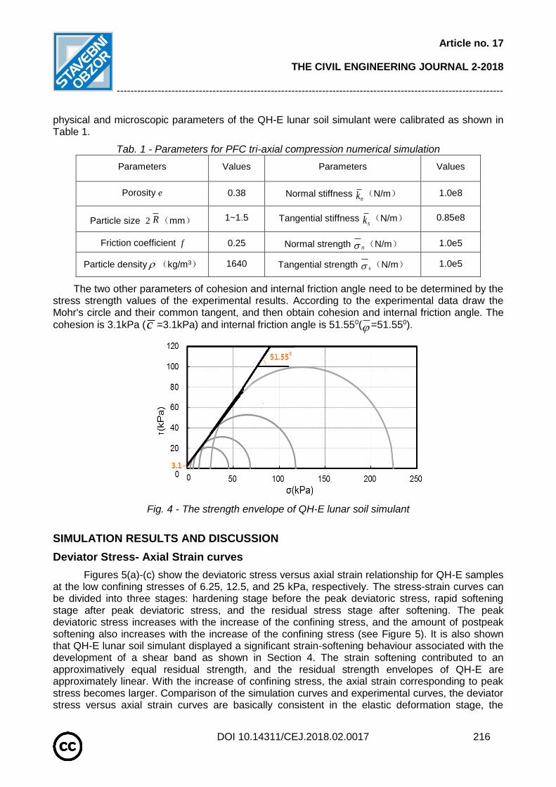
Article no. 17


-----------------------------------------------------------------------------------------------------------------

DOI 10.14311/CEJ.2018.02.0017 216

physical and microscopic parameters of the QH-E lunar soil simulant were calibrated as shown in Table 1.

Tab. 1 - Parameters for PFC tri-axial compression numerical simulation

Parameters Values Parameters Values

Porosity e 0.38 Normal stiffness nk （N/m） 1.0e8

Particle size 2 （mm） 1~1.5 Tangential stiffness sk （N/m） 0.85e8

Friction coefficient f 0.25 Normal strength n （N/m） 1.0e5

Particle density （kg/m3） 1640 Tangential strength s （N/m） 1.0e5

The two other parameters of cohesion and internal friction angle need to be determined by the stress strength values of the experimental results. According to the experimental data draw the Mohr's circle and their common tangent, and then obtain cohesion and internal friction angle. The

cohesion is 3.1kPa (c =3.1kPa) and internal friction angle is 51.550( =51.550).

Fig. 4 - The strength envelope of QH-E lunar soil simulant

SIMULATION RESULTS AND DISCUSSION

Deviator Stress- Axial Strain curves

Figures 5(a)-(c) show the deviatoric stress versus axial strain relationship for QH-E samples at the low confining stresses of 6.25, 12.5, and 25 kPa, respectively. The stress-strain curves can be divided into three stages: hardening stage before the peak deviatoric stress, rapid softening stage after peak deviatoric stress, and the residual stress stage after softening. The peak deviatoric stress increases with the increase of the confining stress, and the amount of postpeak softening also increases with the increase of the confining stress (see Figure 5). It is also shown that QH-E lunar soil simulant displayed a significant strain-softening behaviour associated with the development of a shear band as shown in Section 4. The strain softening contributed to an approximatively equal residual strength, and the residual strength envelopes of QH-E are approximately linear. With the increase of confining stress, the axial strain corresponding to peak stress becomes larger. Comparison of the simulation curves and experimental curves, the deviator stress versus axial strain curves are basically consistent in the elastic deformation stage, the

R

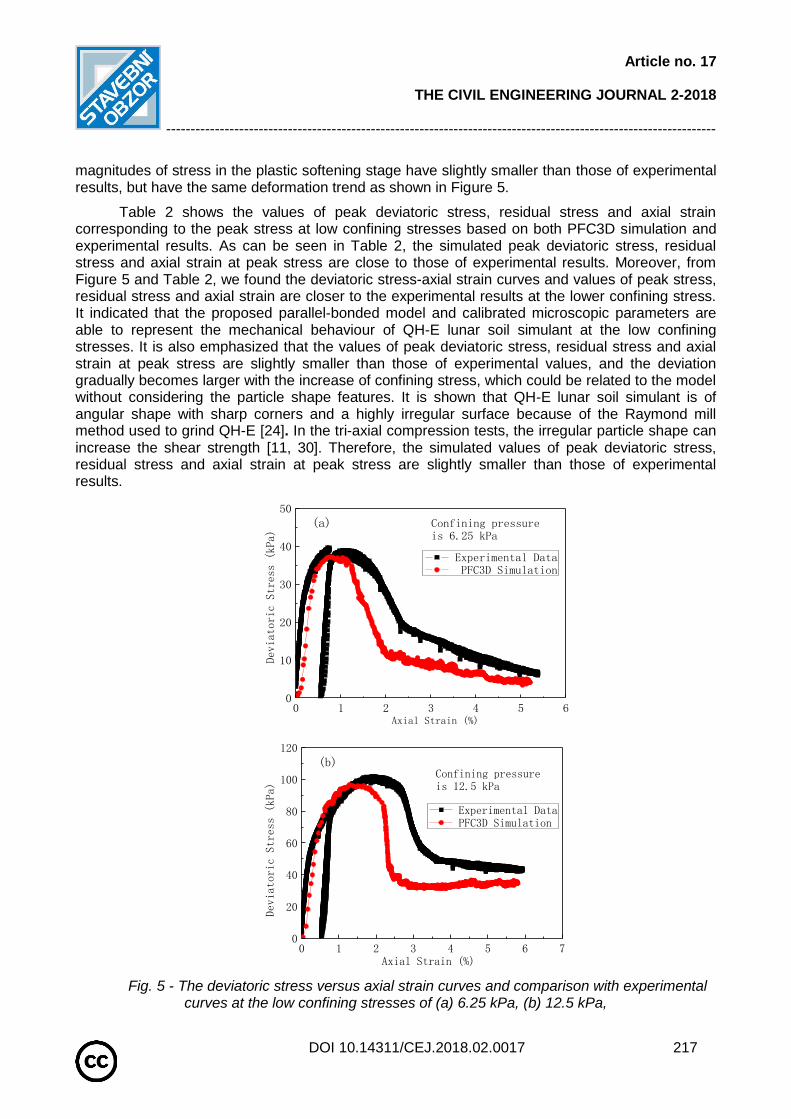
Article no. 17


-----------------------------------------------------------------------------------------------------------------

DOI 10.14311/CEJ.2018.02.0017 217

magnitudes of stress in the plastic softening stage have slightly smaller than those of experimental results, but have the same deformation trend as shown in Figure 5.

Table 2 shows the values of peak deviatoric stress, residual stress and axial strain corresponding to the peak stress at low confining stresses based on both PFC3D simulation and experimental results. As can be seen in Table 2, the simulated peak deviatoric stress, residual stress and axial strain at peak stress are close to those of experimental results. Moreover, from Figure 5 and Table 2, we found the deviatoric stress-axial strain curves and values of peak stress, residual stress and axial strain are closer to the experimental results at the lower confining stress. It indicated that the proposed parallel-bonded model and calibrated microscopic parameters are able to represent the mechanical behaviour of QH-E lunar soil simulant at the low confining stresses. It is also emphasized that the values of peak deviatoric stress, residual stress and axial strain at peak stress are slightly smaller than those of experimental values, and the deviation gradually becomes larger with the increase of confining stress, which could be related to the model without considering the particle shape features. It is shown that QH-E lunar soil simulant is of angular shape with sharp corners and a highly irregular surface because of the Raymond mill method used to grind QH-E [24]. In the tri-axial compression tests, the irregular particle shape can increase the shear strength [11, 30]. Therefore, the simulated values of peak deviatoric stress, residual stress and axial strain at peak stress are slightly smaller than those of experimental results.

0 1 2 3 4 5 60

10

20

30

40

50

Confining pressure is 6.25 kPa

Devi

ator

ic S

tres

s (k

Pa)

Axial Strain (%)

Experimental Data PFC3D Simulation

(a)

0 1 2 3 4 5 6 70

20

40

60

80

100

120


Deviatoric Stress (kPa)

Axial Strain (%)


(b)

Fig. 5 - The deviatoric stress versus axial strain curves and comparison with experimental curves at the low confining stresses of (a) 6.25 kPa, (b) 12.5 kPa,

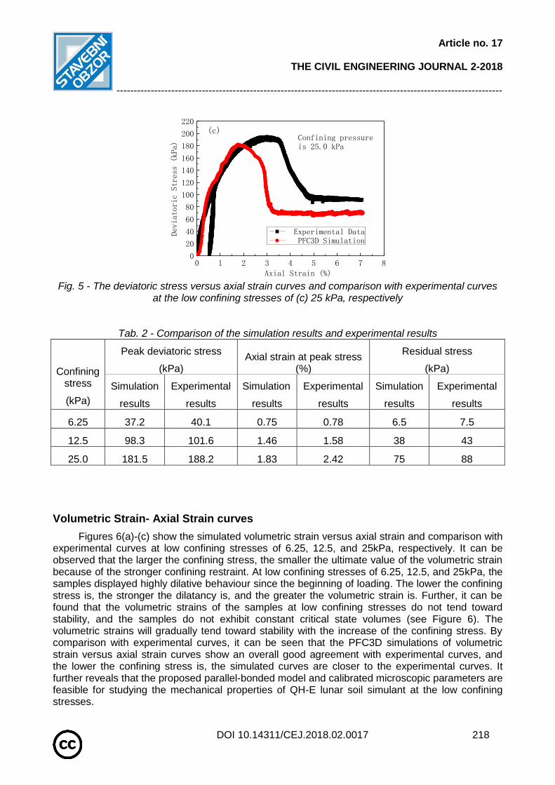
Article no. 17


-----------------------------------------------------------------------------------------------------------------

DOI 10.14311/CEJ.2018.02.0017 218

0 1 2 3 4 5 6 7 80

20

40

60

80

100

120

140

160

180

200

220

Devi

ator

ic S

tres

s (k

Pa)

Axial Strain (%)



(c)

Fig. 5 - The deviatoric stress versus axial strain curves and comparison with experimental curves

at the low confining stresses of (c) 25 kPa, respectively

Tab. 2 - Comparison of the simulation results and experimental results

Confining stress

(kPa)

Peak deviatoric stress

(kPa) Axial strain at peak stress

(%)

Residual stress

(kPa)

Simulation

results

Experimental

results

Simulation

results

Experimental

results

Simulation

results

Experimental

results

6.25 37.2 40.1 0.75 0.78 6.5 7.5

12.5 98.3 101.6 1.46 1.58 38 43

25.0 181.5 188.2 1.83 2.42 75 88

Volumetric Strain- Axial Strain curves

Figures 6(a)-(c) show the simulated volumetric strain versus axial strain and comparison with experimental curves at low confining stresses of 6.25, 12.5, and 25kPa, respectively. It can be observed that the larger the confining stress, the smaller the ultimate value of the volumetric strain because of the stronger confining restraint. At low confining stresses of 6.25, 12.5, and 25kPa, the samples displayed highly dilative behaviour since the beginning of loading. The lower the confining stress is, the stronger the dilatancy is, and the greater the volumetric strain is. Further, it can be found that the volumetric strains of the samples at low confining stresses do not tend toward stability, and the samples do not exhibit constant critical state volumes (see Figure 6). The volumetric strains will gradually tend toward stability with the increase of the confining stress. By comparison with experimental curves, it can be seen that the PFC3D simulations of volumetric strain versus axial strain curves show an overall good agreement with experimental curves, and the lower the confining stress is, the simulated curves are closer to the experimental curves. It further reveals that the proposed parallel-bonded model and calibrated microscopic parameters are feasible for studying the mechanical properties of QH-E lunar soil simulant at the low confining stresses.

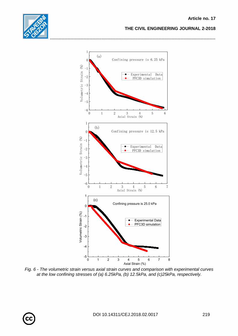
Article no. 17


-----------------------------------------------------------------------------------------------------------------

DOI 10.14311/CEJ.2018.02.0017 219

0 1 2 3 4 5 6-6

-5

-4

-3

-2

-1

0

1


Volumetric Strain (%)

Axial Strain (%)

Experimental Data PFC3D simulation

(a)

0 1 2 3 4 5 6 7-6

-5

-4

-3

-2

-1

0

1


Volumetric Strain (%)

Axial Strain (%)

Experimental Data PFC3D simulation

(b)

0 1 2 3 4 5 6 7 8-5

-4

-3

-2

-1

0

1

Volu

metr

ic S

train

(%

)

Axial Strain (%)

Experimental Data

PFC3D simulation

Confining pressure is 25.0 kPa(c)

Fig. 6 - The volumetric strain versus axial strain curves and comparison with experimental curves

at the low confining stresses of (a) 6.25kPa, (b) 12.5kPa, and (c)25kPa, respectively.

Article no. 17


-----------------------------------------------------------------------------------------------------------------

DOI 10.14311/CEJ.2018.02.0017 220

Effects of porosity and friction coefficient on stress-strain curves

Figure 7 shows the deviatoric stress and axial strain relationship at different porosities and friction coefficients for the same confining stress of 25.0kPa, respectively. As seen in Figure 7, the peak deviatoric stress and residual stress increased in the stress-strain curves with increasing the friction coefficient, whereas decreased with increasing the porosity, and the initial elastic modulus also increased slightly with increasing the friction coefficient or decreasing the porosity. Zou et al. (2008) studied the effect of micro-parameters on the statics characteristic of lunar soil at the conventional confining stress through PFC3D simulation of tri-axial compression test. Their simulation results show that with increasing the friction coefficient, the peak stress increases obviously, and it increases slightly with increasing the particle contact stiffness. While the peak stress decreases with increasing the porosity. The present results indicate that the effects of the porosity and the friction coefficient on the peak stress of QH-E lunar soil simulant at the low confining stress are the same as those at the conventional confining stress by Zou et al. [29].

Table 3 presents a quantitative relationship for the effects of friction coefficient and porosity on the peak stress, residual stress and axial strain corresponding to the peak stress. The peak stress, residual stress and axial strain corresponding to the peak stress are obviously increased with the decrease of the porosity, the peak deviator stress increased obviously from 87.5 to 466.2kPa, the residual stress increased from 36.5 to 156.5kPa, and the axial strain corresponding to this peak stress also increased from 1.35% to 2.25% when the porosity decreased from 0.42 to 0.3 at the same confining stress of 25.0kPa. The effect of friction coefficient is not as obvious as those of the porosity, the peak deviator stress increased from 172.4 to 205.0kPa and the residual stress increased from 67.5 to 77.6kPa when the friction coefficient increased from 0.20 to 0.40, while the change of the axial strain corresponding to the peak stress is very small (from 1.77% to 1.85%) as shown in Table 3.

It can be seen from Figure 7 that the porosity and friction coefficient can obviously affect the peak strength of QH-E lunar soil simulant, and porosity has a stronger effect on the peak strength for tri-axial compression simulation at low confining stress. It indicates that the requirements of macro-mechanical strength can be realized by adjusting the micro-parameters. In general, the initial porosity of the sample is given, so the requirement of the peak strength of tested sample can be achieved by changing the friction coefficient.

0 1 2 3 4 5 6 7 80

100

200

300

400

500

600

Deviatoric Stress (kPa)

Axial Strain (%)

e=0.42 e=0.38 e=0.35 e=0.30

Porosity

Confining Pressure is 25.0 kPa

Fig. 7 - The deviatoric stress and axial strain relationships at different (a) porosities

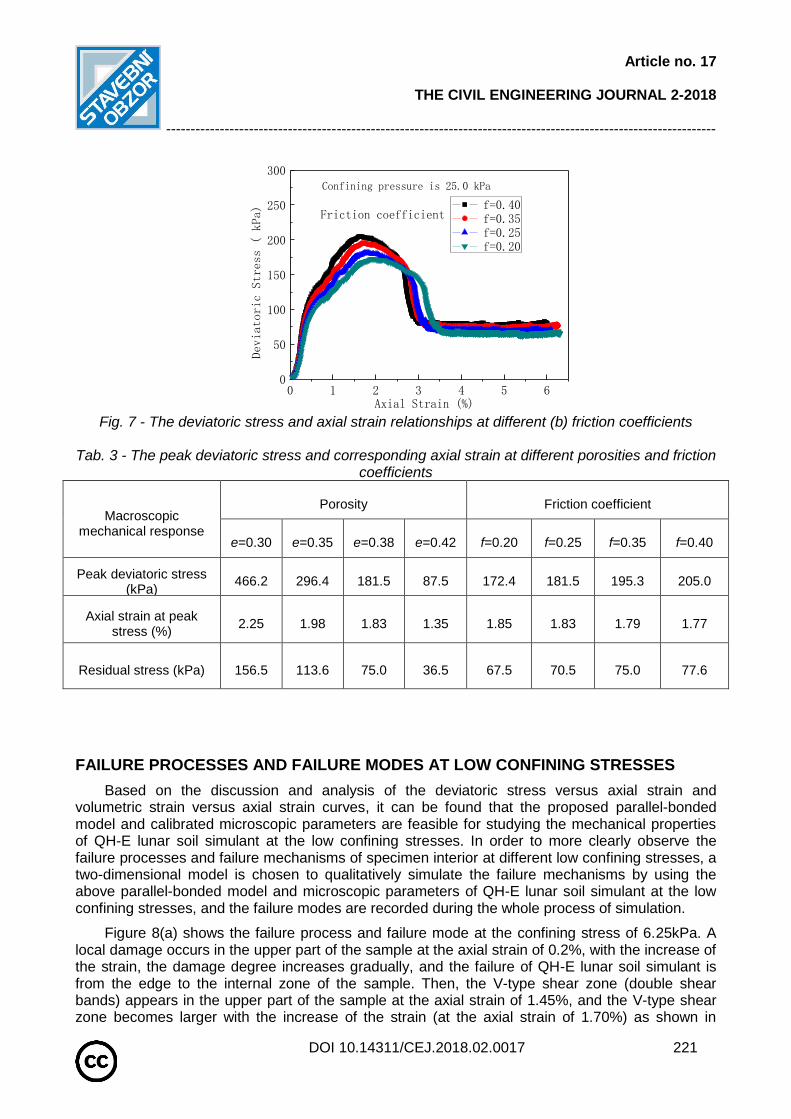
Article no. 17


-----------------------------------------------------------------------------------------------------------------

DOI 10.14311/CEJ.2018.02.0017 221

0 1 2 3 4 5 60

50

100

150

200

250

300

Deviatoric Stress ( kPa)

Axial Strain (%)

f=0.40 f=0.35 f=0.25 f=0.20


Friction coefficient

Fig. 7 - The deviatoric stress and axial strain relationships at different (b) friction coefficients

Tab. 3 - The peak deviatoric stress and corresponding axial strain at different porosities and friction

coefficients

Macroscopic mechanical response

Porosity Friction coefficient

e=0.30 e=0.35 e=0.38 e=0.42 f=0.20 f=0.25 f=0.35 f=0.40

Peak deviatoric stress (kPa)

466.2 296.4 181.5 87.5 172.4 181.5 195.3 205.0

Axial strain at peak stress (%)

2.25 1.98 1.83 1.35 1.85 1.83 1.79 1.77

Residual stress (kPa) 156.5 113.6 75.0 36.5 67.5 70.5 75.0 77.6

FAILURE PROCESSES AND FAILURE MODES AT LOW CONFINING STRESSES

Based on the discussion and analysis of the deviatoric stress versus axial strain and volumetric strain versus axial strain curves, it can be found that the proposed parallel-bonded model and calibrated microscopic parameters are feasible for studying the mechanical properties of QH-E lunar soil simulant at the low confining stresses. In order to more clearly observe the failure processes and failure mechanisms of specimen interior at different low confining stresses, a two-dimensional model is chosen to qualitatively simulate the failure mechanisms by using the above parallel-bonded model and microscopic parameters of QH-E lunar soil simulant at the low confining stresses, and the failure modes are recorded during the whole process of simulation.

Figure 8(a) shows the failure process and failure mode at the confining stress of 6.25kPa. A local damage occurs in the upper part of the sample at the axial strain of 0.2%, with the increase of the strain, the damage degree increases gradually, and the failure of QH-E lunar soil simulant is from the edge to the internal zone of the sample. Then, the V-type shear zone (double shear bands) appears in the upper part of the sample at the axial strain of 1.45%, and the V-type shear zone becomes larger with the increase of the strain (at the axial strain of 1.70%) as shown in

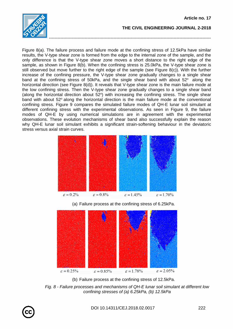
Article no. 17


-----------------------------------------------------------------------------------------------------------------

DOI 10.14311/CEJ.2018.02.0017 222

Figure 8(a). The failure process and failure mode at the confining stress of 12.5kPa have similar results, the V-type shear zone is formed from the edge to the internal zone of the sample, and the only difference is that the V-type shear zone moves a short distance to the right edge of the sample, as shown in Figure 8(b). When the confining stress is 25.0kPa, the V-type shear zone is still observed but move further to the right edge of the sample (see Figure 8(c)). With the further increase of the confining pressure, the V-type shear zone gradually changes to a single shear band at the confining stress of 50kPa, and the single shear band with about 52o along the horizontal direction (see Figure 8(d)). It reveals that V-type shear zone is the main failure mode at the low confining stress. Then the V-type shear zone gradually changes to a single shear band (along the horizontal direction about 52o) with increasing the confining stress. The single shear band with about 52o along the horizontal direction is the main failure mode at the conventional confining stress. Figure 9 compares the simulated failure modes of QH-E lunar soil simulant at different confining stress with the experimental observations. As seen in Figure 9, the failure modes of QH-E by using numerical simulations are in agreement with the experimental observations. These evolution mechanisms of shear band also successfully explain the reason why QH-E lunar soil simulant exhibits a significant strain-softening behaviour in the deviatoric stress versus axial strain curves.

(a) Failure process at the confining stress of 6.25kPa.

(b) Failure process at the confining stress of 12.5kPa.

Fig. 8 - Failure processes and mechanisms of QH-E lunar soil simulant at different low confining stresses of (a) 6.25kPa, (b) 12.5kPa

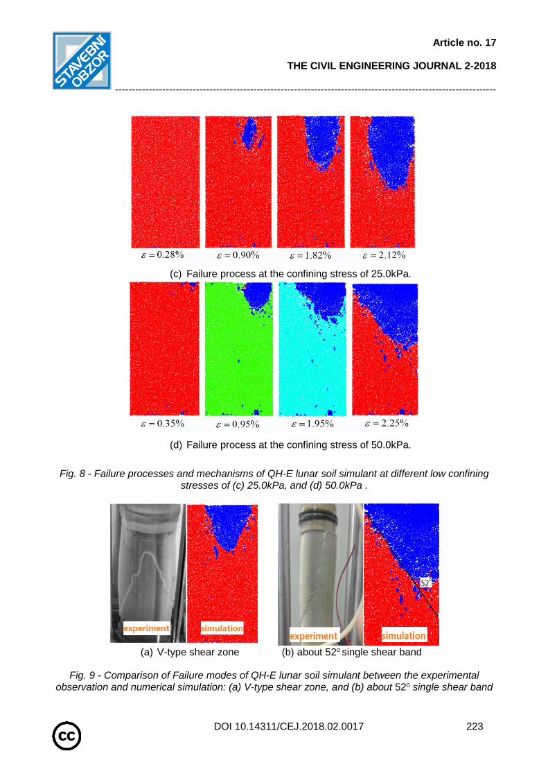
Article no. 17


-----------------------------------------------------------------------------------------------------------------

DOI 10.14311/CEJ.2018.02.0017 223

(c) Failure process at the confining stress of 25.0kPa.

(d) Failure process at the confining stress of 50.0kPa.

Fig. 8 - Failure processes and mechanisms of QH-E lunar soil simulant at different low confining

stresses of (c) 25.0kPa, and (d) 50.0kPa .

(a) V-type shear zone (b) about 52o single shear band

Fig. 9 - Comparison of Failure modes of QH-E lunar soil simulant between the experimental observation and numerical simulation: (a) V-type shear zone, and (b) about 52o single shear band

Article no. 17


-----------------------------------------------------------------------------------------------------------------

DOI 10.14311/CEJ.2018.02.0017 224

CONCLUSION

DEM numerical simulations are carried out to investigate the strength properties and failure modes of QH-E lunar soil simulant at the low confining stress. The effects of porosity and friction coefficient on strength properties of QH-E samples are also discussed. The major findings are as follows:

At low confining stress, the values of peak deviatoric stress, residual stress and axial strain corresponding to the peak stress show an overall good agreement with experimental results, and these values are closer to the experimental values at the lower confining stress. In addition, the deviator stress vs. axial strain and volumetric stress vs. axial strain curves from the present numerical simulations are also similar to those curves from the experimental tests. Therefore, at low confining stress, the proposed model and calibrated microscopic parameters are suitable for simulation the mechanical properties of QH-E lunar soil simulant.

Both the porosity and friction coefficient can affect the peak strength of QH-E lunar soil simulant, and porosity has a stronger effect on the peak strength for tri-axial compression simulation at low confining stress. The peak stress, residual stress and axial strain corresponding to the peak stress obviously decrease with the increase of the porosity, while these values slightly increase with the increase of the friction coefficient at low confining stress.

At the low confining stress, the V-type shear zone (double shear bands) is the main failure mode. Then the V-type shear zone gradually changes to a single shear band (along the horizontal direction about 52o) with the increase of the confining stress. These evolution mechanisms of shear band are in agreement with experimental observation and explain the reason that QH-E lunar soil simulant exhibits a significant strain-softening behaviour.

The above results based on DEM simulation provide the important information about the strength properties and failure modes of QH-E lunar soil simulant at the low confining stress. However, it is emphasized that the current results are obtained under a special contact constitutive model without considering the shape and size distribution of actual particles. Due to the QH-E lunar soil simulant of angular shape with sharp corners and a highly irregular surface, a more detailed PFC simulation based on a more suitable constitutive model is necessary for a more accurate understanding of mechanical properties of QH-E lunar soil simulant.

ACKNOWLEDGEMENTS

The authors would like to gratefully acknowledge the financial support provided by the National Natural Science Foundation of China (NSFC, Grant No. 51079075).

REFERENCES

[1] Hasan, A. and Alshibli, K.A. (2010), “Discrete element modeling of strength properties of Johnson

Space Center (JSC-1 A) lunar regolith simulant”, Journal of Aerospace Engineering, 23(3), 157-165. [2] Heiken, G. H., Vaniman,D. T., French, B. M. (1991), “Lunar sourcebook –A user's guide to the

moon”, Cambridge University Press, Cambridge, U.K., 475-594.

[3] Carrier, W. D. (2003).“Particle size distribution of lunar soil”, Journal of Geotechnicaland

Geoenvironmental Engineering, 129(10), 956-959.

[4] Rickman, D., Hoelzer, H., Carpenter, P., Sibille, L., Howard, R. and Owens, C. (2007), “A

quantitative method for evaluating regolith simulants.”SpaceTechnology and Applications International

Forum-STAIF, American Institute of Physics, 957-963.

[5] Enrique, R., Allen, W., Alan, E., and Carolyn, Y. (2009), “Flow ability of JSC-1A”, Research Rep.

NASA/TM-2009-215625.

Article no. 17


-----------------------------------------------------------------------------------------------------------------

DOI 10.14311/CEJ.2018.02.0017 225

[6] Arslan, H., Batiste, S. and Sture, S. (2010), “Engineering properties of lunar soilsimulant JSC-1A”,

Journal of Aerospace Engineering, 23(1), 70-83.

[7] Jiang, M.J., Zheng, M. and Wang, C. (2012), “Distinct element analysis of shear band of lunar soil in

biaxial tests”, Rock and Soil Mechanics, 33(12), 3801-3809. (in Chinese)

[8] Jiang, M.J. and Shen, Z.F. (2013), “Thornton C. Microscopic contact model of lunar regolith for high

efficiency discrete element analyses”, Computers and Geotechnics, 54, 104-116.

[9] Somrit, C. and Nakagawa, M. (2006), “Simulation of agglutinates formation”, Earth and Space,

188(35), 1-7.

[10] Tryana, V.G. and Masami, N. (2008), “Modeling of agglutinates and its mechanical properties”,

Earth and Space 2008: Engineering, Science, Construction, and Operations in Challenging Environments.

Long Beach: ASCE, 1-8.

[11] Lee, S.J., Hashashi, Y.M.A., Wilkinson, R.A. and Agui, J.H. (2010), “Simulation of experimental

tests on the JSC-1A lunar soil simulant with polyhedral discrete elements”, Earth and Space, 208-216.

[12] Katagirl, J., Matsushima, T., Yamada, Y., Tsuchiyama, A., Nakano, T., Uesugi, K., Ohtake, M. and

Saiki, K. (2015), “Investigation of 3D grain shape characteristics of lunar soil retrieved in Apollo 16 using

image-based discrete-element modeling”, Journal of Aerospace Engineering, 28(4), 04014092.

[13] Matsushima, T., Katagiri, J., Uesugi, K., Tsuchiyama, A. and Nakano, T. (2006), “Image-based

modeling of lunar soil simulant for 3D DEM simulations”, Earth and Space 2006: Engingeering, Construction,

and Operations in Challenging Environment. Houston: ASCE, 1-8.

[14] Matsushima, T., Katagiri, J., Uesugi, K., Tsuchiyama, A. and Nakano, T. (2009), “3D shape

characterization and image-based DEM simulation of the lunar soil simulant FJS-1”, Journal of Aerospace

Engineering, 22(1), 15-23.

[15] Nakashima, H., Fujii, H., Oida, A., Momozu, M., Kanamori, H., Aoki, S., Yokoyama, T., Shimizu, H.,

Miyasaka, J. and Ohdio, K. (2010), “Discrete element method analysis of single wheel performance for a

small lunar rover on sloped terrain”, Journal of Terramechanics, 47, 307-321.

[16] Knuth, M.A., Johnson, J.B., Hopkins, M.A., Sullivan, R.J. and Moore, J.M. (2012), “Discrete element

modeling of Mars Exploration Rover wheel in granular material”, Journal of Terramechanics, 49, 27-36.

[17] Smith, W. and Peng, H. (2013), “Modeling of wheel-soil interaction over rough terrain using the

discrete element method”, Journal of Terramechanics, 50, 277-287.

[18] Zou, M., Fan, S.C., Shi, R.Y., Yang, Y.J. and Li, J.Q. (2015), “Effect of gravity on the mechanical

properties of lunar regolith tested using a low gravity simulation device”, Journal of Terramechanics, 60, 11-

22.

[19] Li, W., Huang, Y., Cui, Y., Dong, S.J. and Wang, J. (2010), “Trafficability analysis of lunar mare

terrain by means of the discrete element method for wheeled rover locomotion”, Journal of Terra-mechanics,

47(3), 161-172.

[20] Alshibli, K. A. and Hasan, A. (2009), “Strength Properties of JSC-1A Lunar Regolith Simulant”,

Journal of Geotechnical and Geoenvironmental Engineering, 135, 673-679.

[21] Klosky, J.L., Sture, S., Ko, H.Y. and Barnes, F. (2000), “Geotechnical Behavior of JSC-1 Lunar Soil

Simulant”, Journal of Aerospace Engineering, 13(4), 133-138.

[22] Nakashima, H., Shioji, Y., Tateyama, K., Aoki, S., Kanamori, H. and Yokoyama, T. (2008), “Specific

cutting resistance of lunar regolith simulant under low gravity conditions”, Journal of Space Engineering,

1(1), 58-68.

[23] Yu, H. and Hu, Z. (2014), “Mechanical characteristics of a lunar regolith simulant at low confining

pressure”, Environmental Earth Sciences, 71, 3697–3703.

[24] Zou, W. L., Li, Y.L., Cheng, L., Zhang, J.F. and Wang, X.Q. (2016), “Mechanical properties of QH-E lunar soil simulant at low confining stresses”, ASCE, Journal of Aerospace Engineering, 29(2), 04015036. [25] Belheine, N., Plassiard, J.P., Donzé, F.V., Darve, F. and Seridi, A. (2009), “Numerical simulation of

drained triaxial test using 3D discrete element modeling”, Computers and Geotechnics, 36(1-2), 320-331.

[26] Willman, B.M., Boles, W.B., McKay, D.S. and Allen, C.C. (1995), “Properties of Lunar Soil Simulant

JSC-1”, Journal of Aerospace Engineering, 8(2), 77–87.

[27] Hicher, P.Y. and Chang, C.S. (2008), “A constitutive model for lunar soil”, Earth and Space, 3-8.

Article no. 17


-----------------------------------------------------------------------------------------------------------------

DOI 10.14311/CEJ.2018.02.0017 226

[28] Jiang, M.J., Yu, H.S. and Harris, D. (2005), “A novel discrete model granular material incorporating

rolling resistance”, Computers and Geotechnics, 32(4), 340-357.

[29] Zou, M., Li, J.Q., Jia, Y., Ren, L.Q. and Li, Y.W. (2008), “Statics characteristics of lunar soil by DEM

simulation”, Journal of Jilin University, 38(2), 383-387. (in Chinese)

[30] Zhao, T., Dai, F., Xu, N.W, Liu, Y. and Xu, Y. (2015), “A composite particle model for non-spherical

particles in DEM simulations”, Grannular Matter, 17, 763-774.

Article no. 18


-----------------------------------------------------------------------------------------------------------------

DOI 10.14311/CEJ.2018.02.0018 227

TWO SIMPLIFIED MODELS OF COLUMN WEB PANEL IN SHEAR

Marta Kuříková, František Wald and Kamila Cábová

Czech Technical University in Prague, Faculty of Civil Engineering, Prague, Czech

Republic; email: [email protected]

ABSTRACT

The paper presents behaviour of the column web panel in shear. The finite element method is employed to examine the resistance of a joint with an extended end plate connection. The FE model is validated to results of physical tests and verified by an analytical solution based on existing formulas. Finally, a parametric study is performed. The studied parameters include web panel thickness, bolt position and the column dimensions.

KEYWORDS Web panel in shear, Finite element model, Parametric study, Steel joint, Component method

INTRODUCTION

Numerous studies were executed in last 20 years to analyse the bending resistance of beam-to-column joints. The component method described in EN1993-1-8:2005 [1] was developed for the beam-to-column steel joints between H and I-profiles and loaded in bending and shear. The resistances are determined for separated components. The compression side resistance of the joint is limited by the shear panel resistance. The influence of the size of the web panel to the quality of prediction by simplified models were studied by Standig [2] and Brandonisio [3]. In reality and in general description of component method the web panel and connections are separated. A simplified procedure is offered in EN 1993-1-8:2005, which is condensing the shear panel and connections into one spring. The shear resistance is described in 6.2.6.1.(2) and the acting forces in 5.3.(3). The distribution of deformations/forces to springs is modelled by β factor, which depends on loading conditions. The web panel and the connection are separated in the proposal of the second draft of EN1993-1-8:2017 [4]. Both concepts, separated and integrated, may have an influence on the joint resistance. A comparison of the results of the proposal of the second draft of EN1993-1-8:2017 with the separated solution according to EN1993-1-8:2005 with the condensed solution to the component based FEM (CBFEM) on the bending moment resistance is prepared for an unsymmetrical joint with the extended end plate connection.

EXPERIMENTAL STUDY

Several experiments were examined to obtain the resistance of the column web panel and to verify the joint’s resistance. The influence of a high axial force is investigated in [5]. An experimental study of the web panels fabricated from high-strength steel is presented in [6] and [7].

An experimental programme done by Sheer et al. [8] is introduced. A tested specimen from the experimental programme is chosen and used in the numerical study hereafter.

Article no. 18


-----------------------------------------------------------------------------------------------------------------

DOI 10.14311/CEJ.2018.02.0018 228

Test details

An eaves moment joint loaded by concentrated force as shown in Figure 1a) was tested to study the behaviour of the column web panel in shear. The results are summarised in [8]. The specimen is made of two welded I section with the dimensions shown in Figure 1b). The height of the section is 306 mm, the column web thickness is 2 mm. The width of flanges is 150 mm and the thickness is 3 mm. The yield stress of the column web fyw = 310 MPa and the yield stress of the beam and column flanges fyr = fyc = 232 MPa were obtained from the tensile test.

a) b) Fig. 1 - a) Dimensions of tested joint b) Tested scheme

VALIDATION

For further investigations, RFEA is developed, see [9] and the design resistance is compared with the experiment. The numerical analyses are completed by the RFEM 5.0 (Dlubal RFEM) [10] finite element program system. The purpose of the validation is to verify the behaviour of the column web panel. A similar study referring to a design of haunches is published by authors in [11].

The materials are endowed with non-linear properties. The ideal plastic model with strain hardening is shown in Figure 2. The geometric details of the model in FEA are taken from the experimental measurement and set according to Figure 1. The welds between plates are neglected in order to simplify the FE model. The numerical model is shown in Figure 3 a). The column is fixed at the end while the beam is loaded by a concentrated force at the free edge. The beam is laterally supported to avoid the lateral torsional buckling.

In the numerical model, 4-node quadrilateral shell elements with nodes at its corners are applied with a maximum side length of 10 mm. Six degrees of freedom are in every node: 3 translations (ux, uy, uz) and 3 rotations (φx, φy, φz). Material and geometric nonlinear analysis with imperfections (GMNIA) is applied. Equivalent geometric imperfections are derived from the first buckling mode

Article no. 18


-----------------------------------------------------------------------------------------------------------------

DOI 10.14311/CEJ.2018.02.0018 229

and the amplitude is set according to Annex C EN1993-1-5:2006 [12]. Large deformation analysis is used and the Newton-Raphson method for solving systems of equations is chosen. The number of loading steps is set to 50, the convergence criteria for tolerance to 1.0% and the maximum number of iterations to 50. The first buckling mode of the model is shown in Figure 3 b).

Fig. 2 - Material model used in the numerical model

a) b)

Fig. 3 - a) Numerical model in RFEM b) First buckling mode

Stress [MPa]

Strain [%]

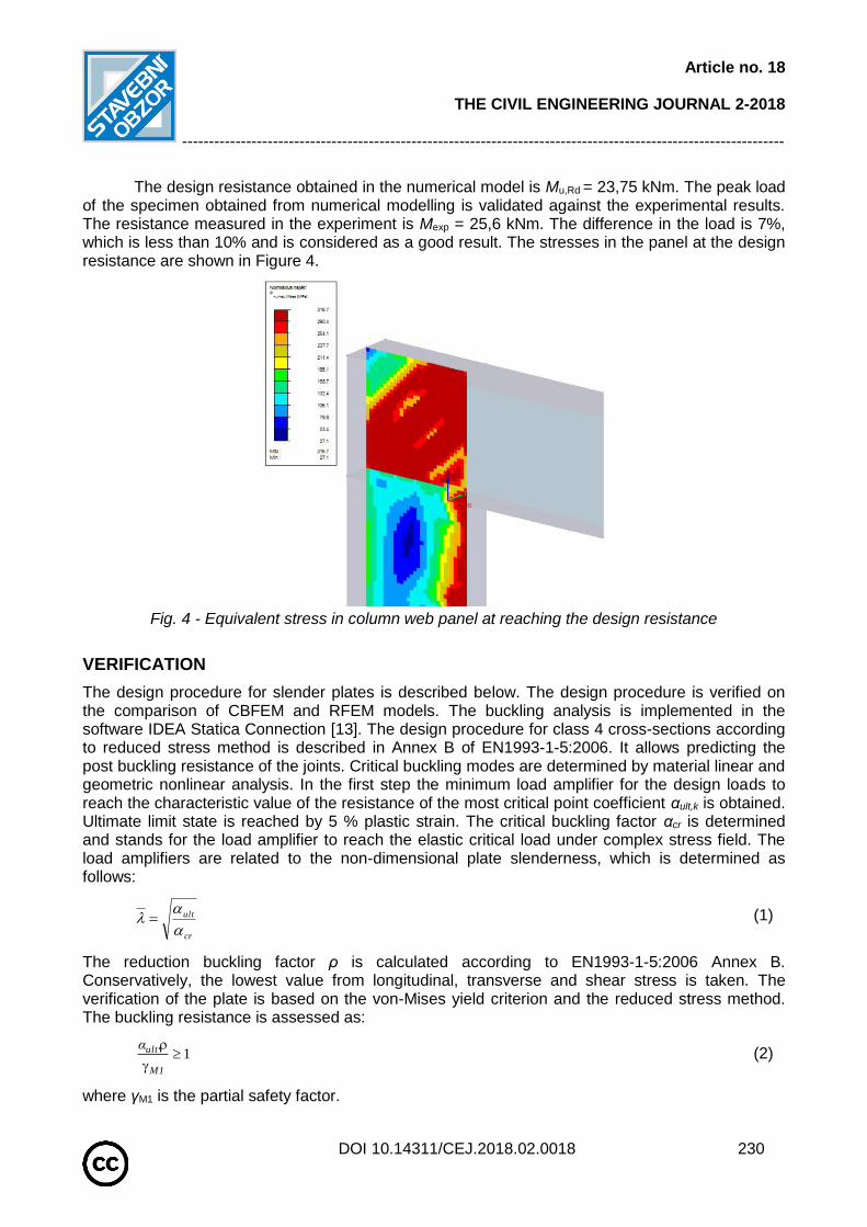
Article no. 18


-----------------------------------------------------------------------------------------------------------------

DOI 10.14311/CEJ.2018.02.0018 230

The design resistance obtained in the numerical model is Mu,Rd = 23,75 kNm. The peak load of the specimen obtained from numerical modelling is validated against the experimental results. The resistance measured in the experiment is Mexp = 25,6 kNm. The difference in the load is 7%, which is less than 10% and is considered as a good result. The stresses in the panel at the design resistance are shown in Figure 4.

Fig. 4 - Equivalent stress in column web panel at reaching the design resistance

VERIFICATION

The design procedure for slender plates is described below. The design procedure is verified on the comparison of CBFEM and RFEM models. The buckling analysis is implemented in the software IDEA Statica Connection [13]. The design procedure for class 4 cross-sections according to reduced stress method is described in Annex B of EN1993-1-5:2006. It allows predicting the post buckling resistance of the joints. Critical buckling modes are determined by material linear and geometric nonlinear analysis. In the first step the minimum load amplifier for the design loads to reach the characteristic value of the resistance of the most critical point coefficient αult,k is obtained. Ultimate limit state is reached by 5 % plastic strain. The critical buckling factor αcr is determined and stands for the load amplifier to reach the elastic critical load under complex stress field. The load amplifiers are related to the non-dimensional plate slenderness, which is determined as follows:

cr

ult

(1)

The reduction buckling factor ρ is calculated according to EN1993-1-5:2006 Annex B. Conservatively, the lowest value from longitudinal, transverse and shear stress is taken. The verification of the plate is based on the von-Mises yield criterion and the reduced stress method. The buckling resistance is assessed as:

1

M1

ult.α (2)

where γM1 is the partial safety factor.

Article no. 18


-----------------------------------------------------------------------------------------------------------------

DOI 10.14311/CEJ.2018.02.0018 231

The RFEM model is compared to the CBFEM model to verify the design procedure. Compared to validated model a simplified material model is used with the yield stress fy = 235 MPa, the tensile strength fu = 360 MPa and Young’s Modulus E = 210 GPa. The resistance of the RFEM model is MRFEM = 21,9 kNm while the resistance of the CBFEM model is calculated as MCBFEM = 21,0 kNm. The results show good agreement in the design resistance. The numerical model is shown in Figure 5a) and the first buckling mode is in Figure 5b).

a) b)

Fig. 5 - a) Numerical model in Idea Statica Connection b) First buckling mode

Sensitivity to the column size

A comparison of results of the proposal of the second draft of EN1993-1-8:2017 with the separated solution according to EN1993-1-8:2005 with the condensed solution to the component based FEM (CBFEM) on the bending moment resistance is prepared for an unsymmetrical joint with the extended end plate connection. The sum of tensile forces limited by a component (beam flange in compression, web panel in shear, column web in compression) with the lowest design resistance according to EN1993-1-8:2005 while the column web panel in shear is not considered directly in the calculation of tensile forces in the second draft and is checked separately. The geometry of the connection is taken from Example C.4 of P398 (2013) but transferred from imperial to continental cross sections IPE and HEB. Geometry of the end plate is in Figure 6, Table 1 and chapter 9.2 in [14].

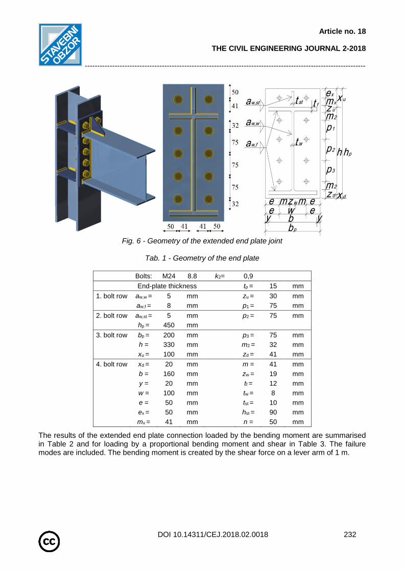
Article no. 18


-----------------------------------------------------------------------------------------------------------------

DOI 10.14311/CEJ.2018.02.0018 232

Fig. 6 - Geometry of the extended end plate joint

Tab. 1 - Geometry of the end plate

Bolts: M24 8.8 k2= 0,9

End-plate thickness

tp = 15 mm

1. bolt row aw,w = 5 mm

zu = 30 mm

aw,f = 8 mm

p1 = 75 mm

2. bolt row aw,st = 5 mm

p2 = 75 mm

hp = 450 mm

3. bolt row bp = 200 mm

p3 = 75 mm

h = 330 mm

m2 = 32 mm

xu = 100 mm

zd = 41 mm

4. bolt row xd = 20 mm

m = 41 mm

b = 160 mm

zw = 19 mm

y = 20 mm

tf = 12 mm

w = 100 mm

tw = 8 mm

e = 50 mm

tst = 10 mm

ex = 50 mm

hst = 90 mm

mx = 41 mm

n = 50 mm

The results of the extended end plate connection loaded by the bending moment are summarised in Table 2 and for loading by a proportional bending moment and shear in Table 3. The failure modes are included. The bending moment is created by the shear force on a lever arm of 1 m.

Article no. 18


-----------------------------------------------------------------------------------------------------------------

DOI 10.14311/CEJ.2018.02.0018 233

Tab. 2: Comparison for joint loaded by bending moment

Beam IPE 330

Loaded by bending moment

Column

CM Difference EN:2017/ EN:2005

CBFEM Difference

Resistance Failure mode


CM/CBFEM

EN:2017 EN:2005 EN:2017 EN:2005

kNm kNm % kNm % %

HEB 200 110 122 CWP Sh. 9,8 110 CWP Sh. 0 -11

HEB 220 124 134 CWP Sh. 7,5 125 CWP Sh. 1 -7

HEB 240 147 153 CWP Sh. 3,9 141 CWP Sh. -4 -9

HEB 260 164 167 CWP Sh. 1,8 150 CWP Sh. -9 -11

HEB 280 180 180 CWP Sh. 0,0 165 CWP Sh. -9 -9

HEB 300 189 189 BF Com. 0,0 180 BS Ten. -5 -5

HEB 320 189 189 BF Com. 0,0 189 BF Com. 0 0

HEB 340 189 189 BF Com. 0,0 189 BF Com.. 0 0

HEB 360 189 189 BF Com. 0,0 189 BF Com. 0 0

HEB 400 189 189 BF Com. 0,0 189 BF Com. 0 0

HEB 450 189 189 BF Com. 0,0 189 BF Com. 0 0

HEB 500 189 189 BF Com. 0,0 189 BF Com.. 0 0

Failure modes: Column web in shear - CWP Sh., Beam flange in compression - BF Com. and Beam stiffener in tension – BS Ten.

Tab. 3 - Comparison of resistances for joint loaded by bending moment and shear

Beam IPE 330

Loaded by M + V

Column


CBFEM Difference



CM/CBFEM

EN:2017 EN:2005 EN:2017 EN:2005

kNm kNm % kNm % %

HEB 200 110 122 CWP Sh. 9,8 120 CWP Sh. 8 -2

HEB 220 124 134 CWP Sh. 7,5 138 CWP Sh. 10 3

HEB 240 147 153 CWP Sh. 3,9 157 BF Com. 6 3

HEB 260 164 167 CWP Sh. 1,8 171 BF Com. 4 2

HEB 280 180 180 CWP Sh. 0 190 BF Com. 5 5

HEB 300 208 208 BF Com.. 0 210 BF Com. 1 1

HEB 320 223 223 BF Com.. 0 228 BF Com. 2 2

HEB 340 226 226 BF Com. 0 243 BF Com. 7 7

HEB 360 229 229 BF Com.. 0 250 BF Com.. 8 8

HEB 400 234 234 BF Com. 0 255 BF Com. 8 8

HEB 450 241 241 BF Com.. 0 263 BF Com. 8 8

HEB 500 248 248 BF Com. 0 271 BF Com. 8 8

Failure modes: Column web in shear - CWP Sh., Beam flange in compression - BF Com.

Article no. 18


-----------------------------------------------------------------------------------------------------------------

DOI 10.14311/CEJ.2018.02.0018 234

Sensitivity to the column web thickness

A parametric study of the column web thickness is presented. A welded cross-section is used for the column and the web panel thickness is changing from 5 to 20 mm. The end-plate and column geometry are summarised in Table 4. The difference from the previous example is highlighted.

Tab. 4 - The end-plate and column geometry

Bolts M24 8.8 k2= 0,9

Column

1. bolt row End-plate thickness

tp = 16 mm

aw,w = 5 mm

zu = 30 mm h = 260 mm

aw,f = 8 mm

p1 = 75 mm bfl = 260 mm

2. bolt row aw,st = 5 mm

p2 = 75 mm tfl = 16 mm

hp = 450 mm

tw = 5 - 20 mm

3. bolt row bp = 200 mm

p3 = 75 mm S235

h = 330 mm

m2 = 32 mm

xu = 100 mm

zd = 41 mm

4. bolt row xd = 20 mm

m = 41 mm

b = 160 mm

zw = 19 mm

y = 20 mm

tf = 12 mm

w = 100 mm

tw = 8 mm

e = 50 mm

tst = 12 mm

ex = 50 mm

hst = 90 mm

mx = 41 mm

n = 50 mm

The results for the extended end plate connection loaded by proportional bending moment and shear are summarised in Table 5. Higher resistance is obtained for a column with a thin web up to 12 mm in CBFEM and in EN1993-1-8:2005. The resistance according to the second draft is underestimated. The distribution of plastic strain in the column web panel with the thickness of 8 mm in CBFEM model is shown in Figure 7.

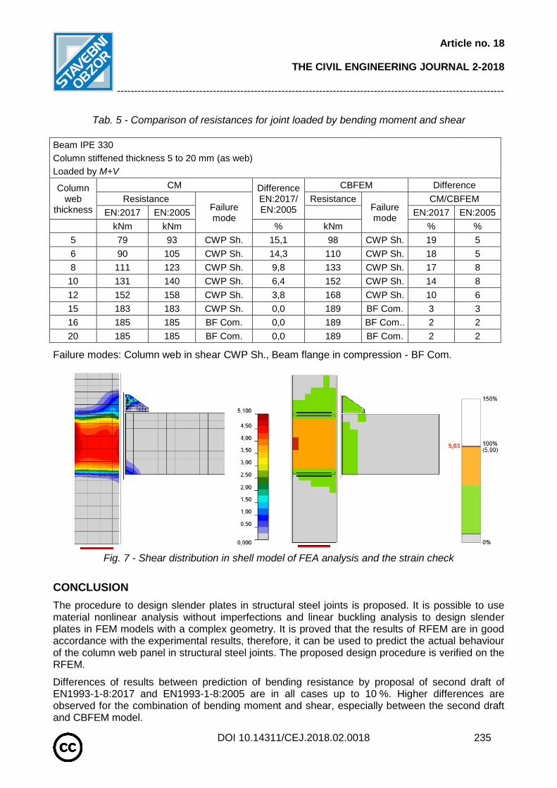
Article no. 18


-----------------------------------------------------------------------------------------------------------------

DOI 10.14311/CEJ.2018.02.0018 235

Tab. 5 - Comparison of resistances for joint loaded by bending moment and shear

Beam IPE 330

Column stiffened thickness 5 to 20 mm (as web)

Loaded by M+V

Column web

thickness


CBFEM Difference



CM/CBFEM

EN:2017 EN:2005

EN:2017 EN:2005

kNm kNm % kNm % %

5 79 93 CWP Sh. 15,1 98 CWP Sh. 19 5

6 90 105 CWP Sh. 14,3 110 CWP Sh. 18 5

8 111 123 CWP Sh. 9,8 133 CWP Sh. 17 8

10 131 140 CWP Sh. 6,4 152 CWP Sh. 14 8

12 152 158 CWP Sh. 3,8 168 CWP Sh. 10 6

15 183 183 CWP Sh. 0,0 189 BF Com. 3 3

16 185 185 BF Com. 0,0 189 BF Com.. 2 2

20 185 185 BF Com. 0,0 189 BF Com. 2 2

Failure modes: Column web in shear CWP Sh., Beam flange in compression - BF Com.

Fig. 7 - Shear distribution in shell model of FEA analysis and the strain check

CONCLUSION

The procedure to design slender plates in structural steel joints is proposed. It is possible to use material nonlinear analysis without imperfections and linear buckling analysis to design slender plates in FEM models with a complex geometry. It is proved that the results of RFEM are in good accordance with the experimental results, therefore, it can be used to predict the actual behaviour of the column web panel in structural steel joints. The proposed design procedure is verified on the RFEM.

Differences of results between prediction of bending resistance by proposal of second draft of EN1993-1-8:2017 and EN1993-1-8:2005 are in all cases up to 10 %. Higher differences are observed for the combination of bending moment and shear, especially between the second draft and CBFEM model.

Article no. 18


-----------------------------------------------------------------------------------------------------------------

DOI 10.14311/CEJ.2018.02.0018 236

The FEA with MITC4 2D shell elements (4 notes, 6 degree of freedom, Mindlin hypotheses) may be expected in this case for the column web panel loaded in shear the most accurate solution. The higher differences in prediction are in case out of a practical application. From the results is clear, that the both analytical models give different results to both sides and oscillate round the FEA results.

ACKNOWLEDGEMENTS

This study was carried out with support by the Technology Agency of the Czech Republic, No. TJ01000045.

REFERENCES

[1] EN 1993-1-8, Eurocode 3: Design of steel structures - Part 1-8: Design of joints, Brussels: CEN,

2005

[2] Standig K.F., Rentschler G.P., Chen W. F., 1975. Tests of bolted beam-to-column flange moment

connections, Fritz Laboratory Reports, Paper 320.

[3] Brandonisio G., De Luca A., Mele E., 2012. Shear strength of panel zone in beam-to-column

connections, Journal of Constructional Steel Research, vol. 71: 129-142

[4] EN 1993-1-8, Eurocode 3: Design of steel structures - Part 1-8: Design of joints, Second draft,

Brussels: CEN, 2017

[5] Fielding D.J., Huang J.S., 1971. Shear in Steel Beam-to-Column Connections, Fritz Laboratory

Reports, Paper 310.

[6] Girão Coelho A.M., Bijlaard F.S.K., Kolstein H., 2009. Experimental behaviour of high-strength steel

web shear panels, Engineering Structures, vol. 31: 1543-1555

[7] Jordão S., Simões da Silva L., Simões R., 2014. Design formulation analysis for high strength steel

welded beam-to-column joints, Engineering Structures, vol. 70: 63-81

[8] Scheer, J., Pasternak, H., Schween, T., 1991. Zum Tragverhalten ausgesteifter Rahmenecken mit

schlanken Stegen, Stahlbau, Vol. 60: 41-48

[9] Trýzna A. 2016. Column web panel in shear, Diploma theses, Czech Technical University in Prague.

[10] Dlubal RFEM 5.0 available at https://www.dlubal.com/en/downloads-and-information

[11] Kurejková M., Wald F., 2017. Design of haunches in structural steel joints, Journal of Civil

Engineering and Management, 23 (6), 765-772.

[12] EN 1993-1-5, Eurocode 3: Design of steel structures - Part 1-5: Plated Structural Elements,

Brussels: CEN, 2006.

[13] Idea Statica 8.2.32 available at https://www.ideastatica.com/downloads/

[14] Wald F., Šabatka L., Bajer M., et al. Benchmark cases for advanced design of structural steel

connections, Prague: CTU Publishing House, 2016.

https://www.dlubal.com/en/downloads-and-information

https://www.ideastatica.com/downloads/

Article no. 19


-----------------------------------------------------------------------------------------------------------------

DOI 10.14311/CEJ.2018.02.0019 237

IMPACT OF CREEP ON FLANGE CLAMPING FORCE

Jan Plášek, Tomáš Ridoško, Jan Ekr, Jiří Kytýr and Roman Gratza

Brno University of Technology, Faculty of Civil Engineering, Institute of

Structural Mechanics, Veveří 331/95, 602 00 Brno, Czech Republic; e-mails:

[email protected], [email protected], [email protected],

[email protected], [email protected]

ABSTRACT

The study presents a numerical analysis of the impact of creep in thermoplastic stub ends on the flange clamping force of a thermoplastic pipe flange connection. The analysis uses available creep modulus values that depend on the stress level, temperature and time. A method that takes the creep modulus into account is proposed and applied to four different detailed variants with the aid of the finite element method. The calculations were performed for selected times at a constant temperature and with static load. The obtained results show that the influence of creep in thermoplastic stub ends causes a substantial reduction in flange clamping force in less than one year.

KEYWORDS Creep modulus, Clamping force, Flange connection, FEM, ANSYS

INTRODUCTION The study deals with a decrease in the initial clamping force of a thermoplastic pipe flange

connection (Figure 1) due to creep [1, 2] in thermoplastic stub ends made from high density polyethylene (PE-HD). The creep in the PE-HD can be described by the creep modulus [3]. The method uses available long term creep modulus values from the EN 1778 standard [4]. The numerical analysis uses the finite element method (FEM) [5, 6]. The study presents a proposed method that takes into account the creep modulus, and applies the method to four different detailed variants. The proposed method considers the exposure time, the stationary temperature and the static load. Another technique that takes into account a creep modulus that is dependent on one temperature, stress field and time was published in [7].

Fig. 1 - Model of a flange connection

FLANGE CONNECTION As can be seen from the depiction of the parts of the flange connection [8] in Figure 2, the

connection is an assembly in which stub ends are welded to pipes which are connected through

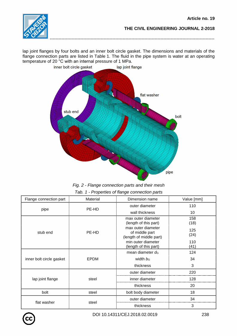
Article no. 19


-----------------------------------------------------------------------------------------------------------------

DOI 10.14311/CEJ.2018.02.0019 238

lap joint flanges by four bolts and an inner bolt circle gasket. The dimensions and materials of the flange connection parts are listed in Table 1. The fluid in the pipe system is water at an operating temperature of 20 °C with an internal pressure of 1 MPa.

Fig. 2 - Flange connection parts and their mesh

Tab. 1 - Properties of flange connection parts

Flange connection part Material Dimension name Value [mm]

pipe PE-HD outer diameter 110

wall thickness 10

stub end PE-HD

max outer diameter (length of this part)

158 (18)

max outer diameter of middle part

(length of middle part)

125 (24)

min outer diameter (length of this part)

110 (41)

inner bolt circle gasket EPDM

mean diameter dG 124

width bG 34

thickness 3

lap joint flange steel

outer diameter 220

inner diameter 128

thickness 20

bolt steel bolt body diameter 18

flat washer steel outer diameter 34

thickness 3

Article no. 19


-----------------------------------------------------------------------------------------------------------------

DOI 10.14311/CEJ.2018.02.0019 239

Creep modulus Creep modulus values (Table 2) for some thermoplastic materials at the exposure time of 1,

10 and 25 years are given in the standard [4]. The creep modulus stated in [4] is defined as the secant creep modulus determined for a given exposure time for a specific stress level and temperature. The creep modulus values of the PE-HD at the temperature of 20 °C for different stress levels and exposure times obtained from the graphs in [4] are given in Table 2.

Tab. 2 - Creep modulus values of PE-HD for 20 °C for the times stated in [4]

Stress level [MPa]

Creep modulus values at selected times [MPa]

1 year 10 years 25 years

0.5 307 255 236

1.0 282 229 206

2.0 235 191 170

3.0 204 161 148

4.0 181 140 130

5.0 159 121 113

Clamping force The flanged clamping force is considered according to the EN 12573-4 standard [9]. The

standard defines the flanged clamping force under assembly and operating conditions.

The flanged clamping force FA [N] under assembly conditions is defined as:

N13245341241GGGA πbdπpF (1)

where pG [MPa] is the pressure exerted on the gasket under assembly conditions, dG [mm] is the mean gasket diameter, bG [mm] is the gasket width and π is a mathematical constant. The flange clamping force under assembly conditions (1) approximately corresponds to the product of the gasket area with a default pressure of 1 MPa applied to the gasket. The gasket area is determined approximately as the product of the circle length determined by the mean gasket diameter with the gasket width.

The flanged clamping force FO [N] under operating conditions is defined as:

N200872

341243.8

4

1241

2

3.8

4

2

GG

2

GOO

π

bddπpF (2)

where pO [MPa] is the operating pressure. The flange clamping force under operating conditions (2) corresponds to the product of the operating pressure with the sum of the two areas. The first area is defined by the mean gasket diameter. The other area is half of the gasket area determined in a similar manner as in formula (1) but with the value 3.8 instead of the mathematical constant π. The sum of the areas approximately corresponds to the area of the circle defined by the outer gasket diameter.

Article no. 19


-----------------------------------------------------------------------------------------------------------------

DOI 10.14311/CEJ.2018.02.0019 240

SIMULATIONS Flange clamping force relaxation at the selected time points is calculated with the finite

element method in the ANSYS software package [6]. The finite element mesh is shown in Figure 1 and Figure 2. The SOLID185 linear brick element is used. Surface to surface contacts are defined between the flange connection parts by a pair of contact elements: CONTA174 and TARGE170. Pretension is applied by a PRETS179 element in the middle of the length of each bolt. At this point a cut perpendicular to the bolt axis is defined. The surfaces created by the cut can be shifted towards each other. The result of this shift is a shortening of the bolt, and therefore pretension loading.

Material The thermoplastic parts of the flange connection are made from high density polyethylene

(PE-HD) [8]. The initial creep modulus value E0 = 800 MPa (0 years) at a temperature of 20 °C is considered to be a constant value for all stress levels. The creep modulus curves in relation to stress level at a temperature of 20 °C for exposure times of 1, 10 and 25 years are shown in Figure 3. The curves pass through the creep moduli from Table 2. The curves are in the form of the polynomial functions used in the material model. The creep modulus values for stresses of less than 0.5 MPa are extrapolated, while for stresses greater than 5.0 MPa they are considered to be constant values.

Fig. 3 - The creep modulus values for the three times for 20 °C in relation to stress

100

150

200

250

300

350

0 1 2 3 4 5 6 7

Cre

ep m

odulu

s [M

Pa]

Stress [MPa]

1 year

10 years

25 years

Temperature 20 °C

Article no. 19


-----------------------------------------------------------------------------------------------------------------

DOI 10.14311/CEJ.2018.02.0019 241

The linear elastic model is used for all the thermoplastic parts of the flange connection. The elastic modulus value is considered to be the creep modulus value from the curve (Figure 3) for the mean von Mises stress of a part of geometry. The von Mises stress [1, 2] is often used to predict the yielding of ductile materials. Creep modulus is determined based on knowledge of the stress level. However, that is generally not known in advance, so an iterative procedure is used.

The weighted mean of the von Mises stress value for the selected part is determined from the mean von Mises stress values on elements with a weight corresponding to the volume of the deformed elements. Therefore, the weighted mean von Mises stress value depends on the selection of the part of geometry, during which the aim is to divide the structure into a small number of parts of geometry with an approximately constant stress for each of them.

Model variants The selected four variants of the finite element model of the flange connection, each with a

different selection of monitored parts of geometry, are:

Variant A – one part: the stub end and the pipe are together.

Variant B – two parts: the stub end and the pipe are separate.

Variant C – three parts: the pipe is separate from the stub end, which is divided into two parts.

Variant D – each element is a separate part.

The four variants of the finite element model of the flange connection are solved in the same way in several load steps. First, pretension load equal to the assembly force FA is applied to the bolts in several load steps, with the criss-cross tightening sequence being used. Subsequently, pressure is applied to the internal surface of the pipe, and in the same load step the pretension load of the bolts is increased to the operating force FO. The ends of the model are defined by two cuts perpendicular to the pipe axis. In the first cut all displacements are set to zero. The other cut is closed with the pipe cap. The pipe cap is loaded by internal pressure as an axial load. The axial load corresponds to the assumption in the formula (2).

First, the shortening of the bolts corresponding to the operating force FO is found for the initial creep modulus value E0. Then the obtained shortening of the bolts is set, and the flange clamping force is monitored while creep moduli (Figure 3) depending on exposure times and stress levels are decreased.

The dependence of the creep moduli on the stress field is solved iteratively. The first iteration uses the initial estimated stress values and this is repeated until the input and output stress field are sufficiently similar. Geometric nonlinear static analyses are used.

Results The von Mises stress field at the initial time (0 years) is the same for all variants, see

Figure 4. The von Mises stress fields after the exposure time of 1 year for each variant are shown in Figures 5 to 8. All figures only show the monitored thermoplastic stub ends and the pipes. In the case of variants B (Figure 6) and C (Figure 7) the monitored parts are additionally shifted towards each other and enlarged to show more detail. The same colour scale is used with each image to allow better comparison of the results.

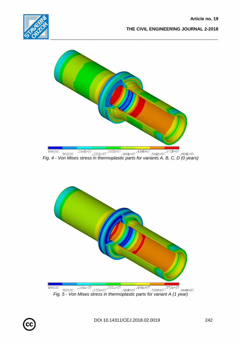
Article no. 19


-----------------------------------------------------------------------------------------------------------------

DOI 10.14311/CEJ.2018.02.0019 242

Fig. 4 - Von Mises stress in thermoplastic parts for variants A, B, C, D (0 years)

Fig. 5 - Von Mises stress in thermoplastic parts for variant A (1 year)

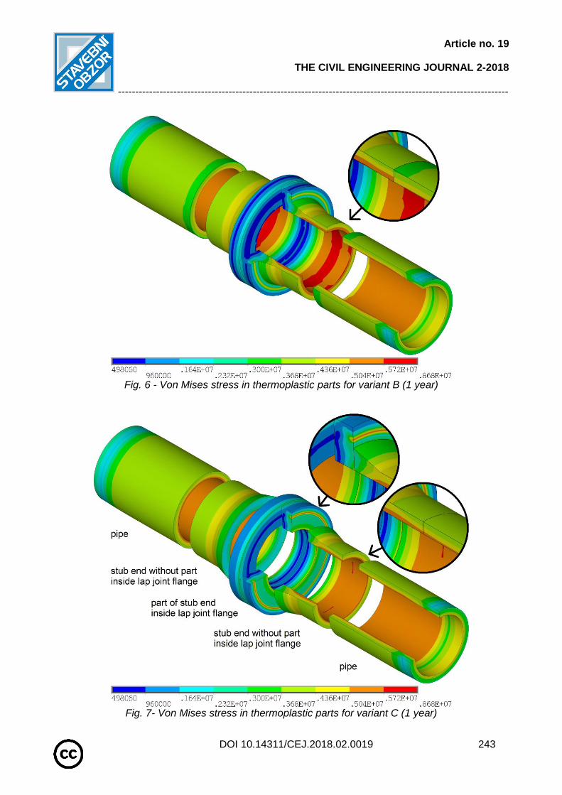
Article no. 19


-----------------------------------------------------------------------------------------------------------------

DOI 10.14311/CEJ.2018.02.0019 243

Fig. 6 - Von Mises stress in thermoplastic parts for variant B (1 year)

Fig. 7- Von Mises stress in thermoplastic parts for variant C (1 year)

Article no. 19


-----------------------------------------------------------------------------------------------------------------

DOI 10.14311/CEJ.2018.02.0019 244

Fig. 8 - Von Mises stress in thermoplastic parts for variant D (1 year)

The results after the first year of exposure show that due to the creep in the thermoplastic material, the stresses are redistributed, extreme stresses are reduced and the variants are different from one another. According to expectations the greatest difference between extreme values is found for variants A (Figure 5) and D (Figure 8). The results also show that in variants B and C the stress field is discontinuous due to the discontinuity of the creep modulus between the individual parts. The stress fields at both ends of the model are affected by boundary conditions.

The von Mises stress values and the clamping force values for the exposure times are listed in Table 3. The mean von Mises stresses from all of the solved variants and times are compared in three monitored parts corresponding to variant C (Figure 7).

According to expectations the same results were obtained for all variants for the calculation at 0 years (Table 3) with the initial creep modulus value. The highest mean von Mises stress found for the monitored parts is in the stub ends without the part inside the lap joint flanges. The smallest mean von Mises stress is in the part of the stub ends inside the lap joint flanges.

Article no. 19


-----------------------------------------------------------------------------------------------------------------

DOI 10.14311/CEJ.2018.02.0019 245

Tab. 3 - Mean von Mises stress and flange clamping force in the monitored parts

Physical quantity

Monitored part Variant Time point [years]

0 1 10 25

mean von Mises stress

[MPa]

part of stub end

inside lap joint flange

A 2.126 1.618 1.607 1.601

B 2.126 1.623 1.601 1.605

C 2.126 1.823 1.845 1.820

D 2.126 1.784 1.794 1.781

stub end without part

inside lap joint flange

A 4.538 4.403 4.511 4.516

B 4.538 4.441 4.469 4.560

C 4.538 4.305 4.315 4.421

D 4.538 4.373 4.395 4.488

pipe

A 4.080 4.186 4.228 4.243

B 4.080 4.175 4.217 4.234

C 4.080 4.200 4.248 4.265

D 4.080 4.229 4.283 4.297

clamping force [kN]

bolts

A 20.087 11.669 10.706 10.642

B 20.087 11.827 11.296 10.698

C 20.087 12.616 12.386 11.625

D 20.087 12.451 12.073 11.394

The flange clamping force decreased by approximately 40% from the initial value with the most significant decrease occurring during the first year of exposure. Over the same period of time the creep modulus values decreased to approximately 260 to 170 MPa from the initial value of 800 MPa. The subsequent decrease in the flange clamping force for exposure times of 10 and 25 years is not significant.

The results of the mean von Mises stress in the monitored parts after the first year of exposure indicate that variant C is different by less than 2.2% and variants A and B are different by less than 9.3% in comparison with the results for the most detailed variant D. At the same time, the results of the flange clamping force value indicate that variant C is different by less than 1.4% and variants A and B are different by less than 6.3% in comparison with the results for the most detailed variant D.

CONCLUSION Due to creep in the thermoplastic parts of the flange connection, there is a significant

decrease in the flange clamping force during the first year of exposure. After this first year, the initial creep modulus decreased by approximately 75% and the flange clamping force by around 40%. According to numerical analysis results it is necessary to check the flange clamping force during the first year of exposure.

The mean von Mises stress and the flange clamping force at all the selected times except the initial time (0 years) for variants A to C were less than 11.5% different in comparison with the most detailed variant D. The results for variant C, which takes into account the three creep modulus values, are comparable with the results for the most detailed and the most demanding variant D. Variant C is sufficiently precise and is usable in practice.

The calculations were performed for the selected times assuming constant temperature and static load. The proposed method uses a creep modulus that takes into account the exposure time, the stationary temperature field and the static load, and can be generally used for other thermoplastic structures.

Article no. 19


-----------------------------------------------------------------------------------------------------------------

DOI 10.14311/CEJ.2018.02.0019 246

ACKNOWLEDGEMENTS

This paper has been prepared under project No. LO1408 "AdMaS UP - Advanced Materials, Structures and Technologies", supported by the Ministry of Education, Youth and Sports of the Czech Republic under "National Sustainability Programme I".

REFERENCES

[1] Jirásek M, Zeman J., 2006. Přetváření a porušování materiálů. Dotvarování, plasticita, lom a

poškození. (Nakladatelství ČVUT, Praha. ISBN: 80-01-03555-7)

[2] Sobotka Z., 1981. Reologie hmot a konstrukcí. (Academia, Praha)

[3] Osswald T. A., Menges G., 2003. Materials Science of Polymers for Engineers. (2nd Edition, Carl

Hanser Verlag, Munich. ISBN: 3-446-22464-5)

[4] EN 1778, 2000. Characteristic values for welded thermoplastics constructions – Determination of

allowable stresses and moduli for design of thermoplastics equipment

[5] Belytschko T., Liu W. K., Moran B., 2000. Nonlinear Finite Elements for Continua and Structures.

(John Wiley & Sons Ltd., New York)

[6] ANSYS Theory Reference 16.0

[7] Plášek J., Ridoško T., Kytýr J., Gratza R., 2013. Časová změna kruhové tuhosti korugovaného

termoplastového kanalizačního potrubí. (Stavební obzor, roč. 2013, č. 03, s. 76-80, ISSN: 1210-4027)

[8] www.simona.de

[9] EN 12573-4, 2000. Welded static non-pressurized thermoplastic tanks. Design and calculation of

flanged joints

Article no. 20


---------------------------------------------------------------------------------------------------------------

DOI 10.14311/CEJ.2018.02.0020 247

PERIODICALLY REPEATING SOUND AS A DISRUPTIVE AGENT IN BUILDINGS

Jaroslav Hejl 1,2

1. Czech Technical University, Faculty of Civil Engineering, Department of

buildings structures, Prague, Thakurova 7, Praha 6 - Dejvice, Czech Republic;

[email protected]

2. University Centre for Energy Efficient Buildings, Trinecka 1024, Bustehrad, Czech Republic

ABSTRACT

This work focuses on subjective perception of disruptive sounds with different harmonic frequencies and parts. It verifies the core of subjective disturbance on basis of a listening test. The effort is to clarify if there is more problematic the issue of clearly audible beats – which is more informative contents issue – or predominantly low frequencies of sound. Clearly audible impulses in sound records are meant by the definition beats in this article – for example drums in the recording. The point of interest is mainly low efficiency of sound insulation against low frequency sound as music with significant beats. The research is restricted only on respondents without hearing difficulties. Based on answers from more than 20 respondents there is conclusion from this paper that the research focus is far from clearance and simplicity. Answers are often very inconsistent and complaints about impossible task were noticed multiple times. In general, however, there is very clear that the problem in disturbance is hidden in low frequencies and with audible beats. The low frequencies are the key disturbance agent in this particular matter.

KEYWORDS Acoustics, Subjective evaluation, Listening test, Low frequency sound

INTRODUCTION Insufficient sound insulation and its connection with low-frequency sound sources in

building acoustics brings a new problem. In reference to this, there is increasing number of user complaints on the clearly audible beats within a noise from neighborhood. Periodically recurring "beats" in music are mostly a low frequency component. The problem is how to effectively decrease transition of these noise components in lightweight multi-layered structures. These lightweight structures are very different from heavyweight in terms of acoustic behavior.

For a multilayer construction we can consider as an illustrative example a wall made of gypsum board on metal frame where the spaces between which are filled with mineral insulation - see Figure 1.

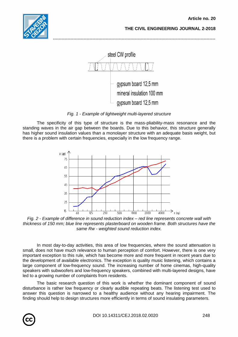
Article no. 20


---------------------------------------------------------------------------------------------------------------

DOI 10.14311/CEJ.2018.02.0020 248

Fig. 1 - Example of lightweight multi-layered structure

The specificity of this type of structure is the mass-pliability-mass resonance and the standing waves in the air gap between the boards. Due to this behavior, this structure generally has higher sound insulation values than a monolayer structure with an adequate basis weight, but there is a problem with certain frequencies, especially in the low frequency range.

Fig. 2 - Example of difference in sound reduction index – red line represents concrete wall with

thickness of 150 mm; blue line represents plasterboard on wooden frame. Both structures have the same Rw - weighted sound reduction index.

In most day-to-day activities, this area of low frequencies, where the sound attenuation is small, does not have much relevance to human perception of comfort. However, there is one very important exception to this rule, which has become more and more frequent in recent years due to the development of available electronics. The exception is quality music listening, which contains a large component of low-frequency sound. The increasing number of home cinemas, high-quality speakers with subwoofers and low-frequency speakers, combined with multi-layered designs, have led to a growing number of complaints from residents.

The basic research question of this work is whether the dominant component of sound disturbance is rather low frequency or clearly audible repeating beats. The listening test used to answer this question is narrowed to a healthy audience without any hearing impairment. The finding should help to design structures more efficiently in terms of sound insulating parameters.

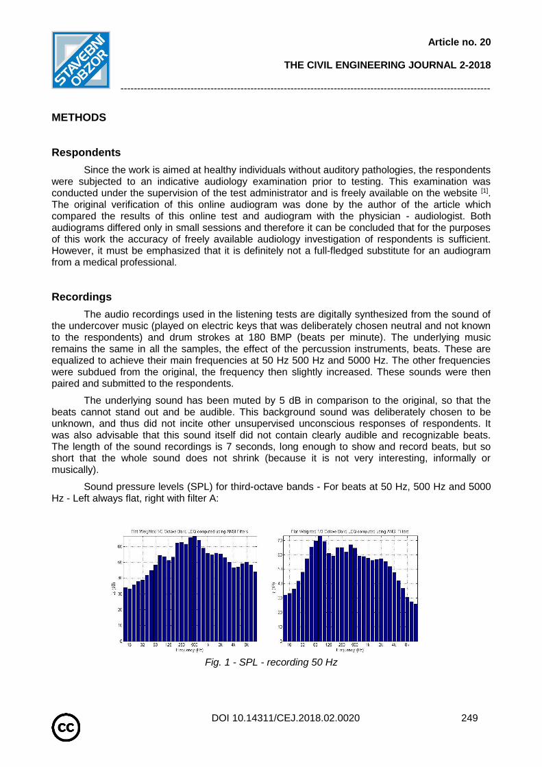
Article no. 20


---------------------------------------------------------------------------------------------------------------

DOI 10.14311/CEJ.2018.02.0020 249

METHODS

Respondents

Since the work is aimed at healthy individuals without auditory pathologies, the respondents were subjected to an indicative audiology examination prior to testing. This examination was conducted under the supervision of the test administrator and is freely available on the website [1]. The original verification of this online audiogram was done by the author of the article which compared the results of this online test and audiogram with the physician - audiologist. Both audiograms differed only in small sessions and therefore it can be concluded that for the purposes of this work the accuracy of freely available audiology investigation of respondents is sufficient. However, it must be emphasized that it is definitely not a full-fledged substitute for an audiogram from a medical professional.

Recordings

The audio recordings used in the listening tests are digitally synthesized from the sound of the undercover music (played on electric keys that was deliberately chosen neutral and not known to the respondents) and drum strokes at 180 BMP (beats per minute). The underlying music remains the same in all the samples, the effect of the percussion instruments, beats. These are equalized to achieve their main frequencies at 50 Hz 500 Hz and 5000 Hz. The other frequencies were subdued from the original, the frequency then slightly increased. These sounds were then paired and submitted to the respondents.

The underlying sound has been muted by 5 dB in comparison to the original, so that the beats cannot stand out and be audible. This background sound was deliberately chosen to be unknown, and thus did not incite other unsupervised unconscious responses of respondents. It was also advisable that this sound itself did not contain clearly audible and recognizable beats. The length of the sound recordings is 7 seconds, long enough to show and record beats, but so short that the whole sound does not shrink (because it is not very interesting, informally or musically).

Sound pressure levels (SPL) for third-octave bands - For beats at 50 Hz, 500 Hz and 5000 Hz - Left always flat, right with filter A:

Fig. 1 - SPL - recording 50 Hz

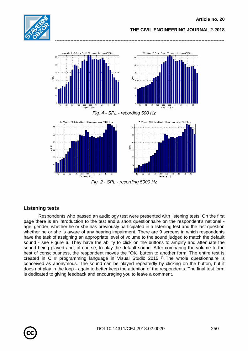
Article no. 20


---------------------------------------------------------------------------------------------------------------

DOI 10.14311/CEJ.2018.02.0020 250



Listening tests

Respondents who passed an audiology test were presented with listening tests. On the first page there is an introduction to the test and a short questionnaire on the respondent's national - age, gender, whether he or she has previously participated in a listening test and the last question whether he or she is aware of any hearing impairment. There are 9 screens in which respondents have the task of assigning an appropriate level of volume to the sound judged to match the default sound - see Figure 6. They have the ability to click on the buttons to amplify and attenuate the sound being played and, of course, to play the default sound. After comparing the volume to the best of consciousness, the respondent moves the "OK" button to another form. The entire test is created in C # programming language in Visual Studio 2015 [3].The whole questionnaire is conceived as anonymous. The sound can be played repeatedly by clicking on the button, but it does not play in the loop - again to better keep the attention of the respondents. The final test form is dedicated to giving feedback and encouraging you to leave a comment.

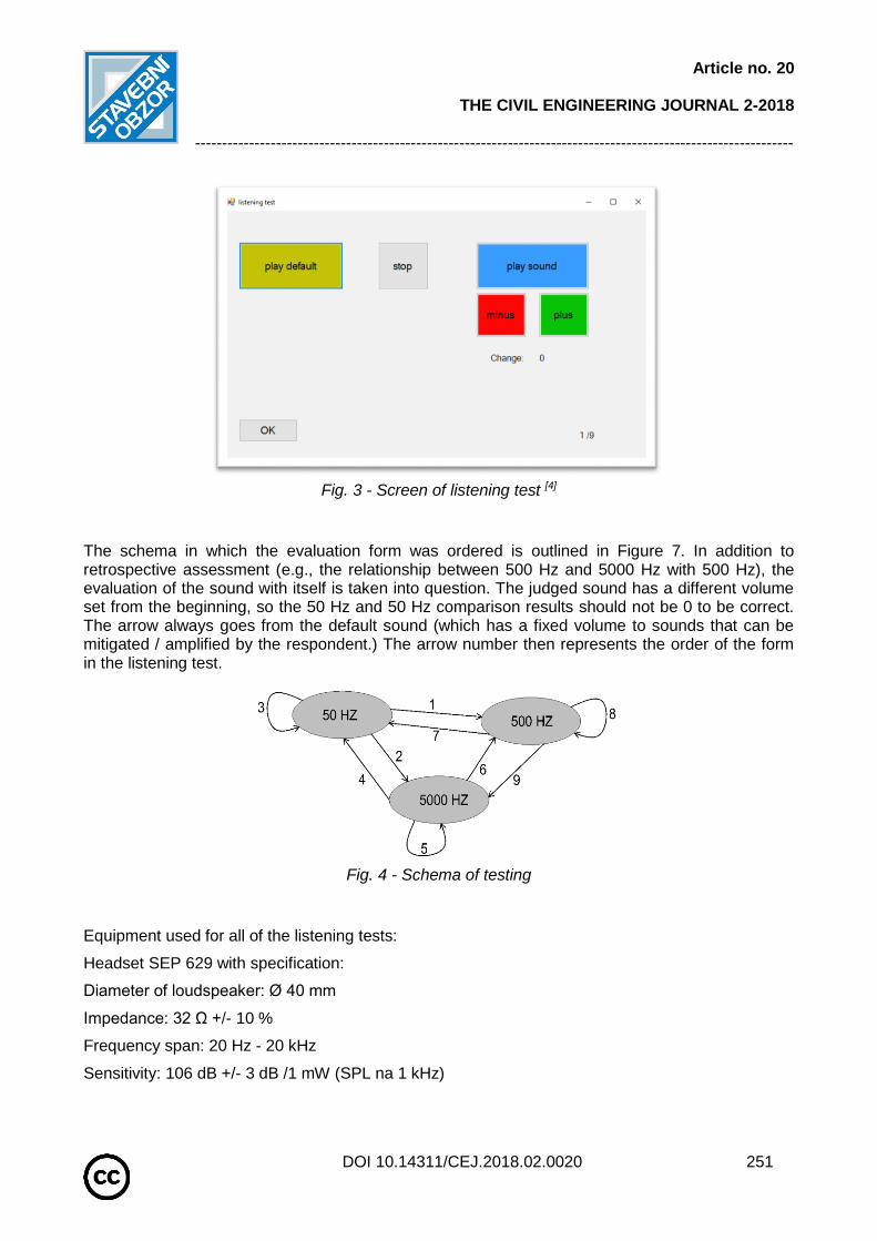
Article no. 20


---------------------------------------------------------------------------------------------------------------

DOI 10.14311/CEJ.2018.02.0020 251

Fig. 3 - Screen of listening test [4]

The schema in which the evaluation form was ordered is outlined in Figure 7. In addition to retrospective assessment (e.g., the relationship between 500 Hz and 5000 Hz with 500 Hz), the evaluation of the sound with itself is taken into question. The judged sound has a different volume set from the beginning, so the 50 Hz and 50 Hz comparison results should not be 0 to be correct. The arrow always goes from the default sound (which has a fixed volume to sounds that can be mitigated / amplified by the respondent.) The arrow number then represents the order of the form in the listening test.

Fig. 4 - Schema of testing

Equipment used for all of the listening tests:

Headset SEP 629 with specification:

Diameter of loudspeaker: Ø 40 mm

Impedance: 32 Ω +/- 10 %

Frequency span: 20 Hz - 20 kHz

Sensitivity: 106 dB +/- 3 dB /1 mW (SPL na 1 kHz)

Article no. 20


---------------------------------------------------------------------------------------------------------------

DOI 10.14311/CEJ.2018.02.0020 252

Tests took place at different places, depending on the respondents' preference. In any case, however, the test was performed within a acoustically insulated room, without other distractions and without significant psychological subtexts.

RESULTS

According the answers from respondent of listening tests there is possible to conclude several things.

In following table there are shown all the raw valid answers. There were also 4 respondents who do not satisfy the preliminary audiology test so their answers are not processed.

Tab. 1 - Sheet with answers from respondents

From the table is clearly visible that the range of answers is quite broad. The conclusion is that it is highly difficult for people to compare different sounds – despite their similarity. Answers depend on each respondent and his preference or maybe better spoken - immunity to particular component of disturbing sound. Therefore, it is not possible to strictly announce that something is true covering all of population.

In the next table there are results already processed by some means. Answers are averaged and adjusted to the same level (nullification of that +5 sound level point in default sound). Also there is added the analyzed sound from sound analyzer, which is very appreciated for objective comparison.

datum number age genderprevious

participation

hearing

problem

50-500

Hz

50-5000

Hz

50-50

Hz

5000-50

Hz

5000-

5000 Hz

5000-500

Hz

500-50

Hz

500-500

Hz

500-5000

Hz03.12.2017 1 24-30 male yes no -3 14 -5 -19 -4 -16 -8 -5 12

03.12.2017 2 50-65 male yes no -1 9 -3 -6 -1 -12 -7 -4 5

03.12.2017 3 50-65 female yes no -2 11 -4 -14 -10 -13 -8 -7 5

03.12.2017 4 24-30 female yes no -5 -7 -6 -7 -4 -6 -9 -5 -11

06.12.2017 5 24-30 male yes no -4 -2 -7 -10 -6 -10 -8 -7 1

24.12.2017 6 30-40 male no no -4 9 -4 -14 -2 -12 -8 -1 8

24.12.2017 7 24-30 male no no -1 16 -4 -17 -4 -16 -10 -5 14

24.12.2017 8 24-30 female no no -6 -5 -8 -9 -7 -9 -10 -4 -5

24.12.2017 9 30-40 male yes no -4 2 -5 -12 -6 -10 -12 -7 1

24.12.2017 10 50-65 female no no 0 13 -4 -19 -4 -14 -9 -4 8

24.12.2017 11 >65 male yes no 0 15 -5 -13 -3 -14 -10 -5 9

28.12.2017 12 30-40 male no no -3 9 -7 -17 -4 -10 -9 -5 8

28.12.2017 13 50-65 female yes no -1 -7 -4 -12 -4 -12 -7 -7 1

28.12.2017 14 24-30 male yes no -6 2 -4 -13 -7 -12 -8 -5 1

28.12.2017 15 30-40 male no no -3 13 -8 -7 -10 -16 -10 -4 5

28.12.2017 16 24-30 female no no -4 16 -3 -10 -1 -6 -8 -7 8

29.12.2017 17 50-65 male yes no -3 11 -4 -13 -5 -14 -8 -5 7

29.12.2017 18 50-65 female no no -2 -8 -4 -14 -4 -11 -8 -6 4

29.12.2017 19 30-40 female no no -3 5 -5 -12 -5 -11 -9 -5 4

29.12.2017 20 24-30 male yes no -4 6 -4 -10 -6 -12 -10 -4 5

frequency comparisoninquiry

comparison of sounds. First (default) sound is louder by 5 point than the second one.

Article no. 20


---------------------------------------------------------------------------------------------------------------

DOI 10.14311/CEJ.2018.02.0020 253

Tab. 2 - Sheet with processed results

The blue columns show the same sound – at this point there is agreement within the answers in respondents themselves and analyzer as well. One decibel is close to the Just Noticeable Difference (JND) for sound level [2]. On the other hand there are significant differences in others columns. In general, however there is clearly visible inclination to evaluate sounds with dominant frequencies of 5000 Hz as the most silent ones and 50 Hz as the loudest one – Comparison 50 Hz and 5000 Hz differs about 18,68 points (respectively 14,05 in case of 5000 Hz and 50 Hz) from real A weighted scale based on analyzer. 1 point in answer sheet responds approximately to 1 dB in sound pressure level based on sound analyzer measurement. The difference between 50 Hz and 500 Hz is insignificant. In exact numbers is in average less than 2,5 points.

CONCLUSION

At the first there must be noticed that the population of respondents is very limited and therefore the statistical significance is not so great. There should be more research and study to confirm and specify these results.

The respondents were relatively accurate in evaluation the same sounds – comparison 50 Hz and 50 Hz for example. However there was big difference in comparison of other sounds. Also there were multiple complaints of almost impossible task to compare such different sounds – although only difference was in frequency of the beats.

Answers had anyway shown that in general there is strong inclination to evaluate beats played in higher frequencies as not so loud as beats played on low frequencies. In other words the hypothesis of low frequencies as the dominant disruptive element is confirmed in this paper. If this conclusion is proven right in further studies and research, it should be comprehend into methodic of design of buildings. Based on these results there is crucial way to increase sound reduction especially on low frequencies in order to achieve better insulation capabilities.

ACKNOWLEDGEMENTS

This work has been supported by the Ministry of Education, Youth and Sports within National Sustainability Program I (NPU I), project No. LO1605 University Centre for Energy Efficient Buildings Sustainability Phase. This work has been also funded by grant no. SGS17/007/OHK1/1T/11 - CTU Prague.

50-500

Hz

50-5000

Hz

50-50

Hz

5000-50

Hz

5000-

5000 Hz

5000-500

Hz

500-50

Hz

500-500

Hz

500-5000

Hz

2,05 10,68 0,11 -7,05 0,11 -6,58 -3,84 -0,11 9,11

1,76 8,18 1,52 3,75 2,43 2,86 1,24 1,48 5,63

70,1 69,9 70,2 74 73 75 68,6 69,7 68,6

-1 -8 0 7 -1 10 -2 1 -5

3,05 18,68 0,11 -14,05 1,11 -16,58 -1,84 -1,11 14,11

74,0 69,0

right answer according sound

analysatordifference between sound

analysator and respondents

average of respondents

standard deviation

from sound analysator: default

(dB)from sound analysator: default -

average(dB)70,1

Article no. 20


---------------------------------------------------------------------------------------------------------------

DOI 10.14311/CEJ.2018.02.0020 254

REFERENCES

[1] Audiocheck. Audio tests. Audiometric test (125-8,000 Hz) (quote from 13.12.2017); Available from http://www.audiocheck.net/testtones_hearingtestaudiogram.php [2] Physclips. UNSW – School of Physics, Sydney, Australia. (quote from 13.12.2017); Available from http://www.animations.physics.unsw.edu.au/jw/dB.htm [3] Software: Microsoft Visual Studio Community 2015, Version 14.0.25431.01 Update 3, Microsoft .NET, Framework, Version 4.7.02556 [4] HEJL, Jaroslav. GUI for listening tests [software]. Ver. 1.01A. [Czech Republic], 2017

http://www.audiocheck.net/testtones_hearingtestaudiogram.php

http://www.animations.physics.unsw.edu.au/jw/dB.htm

Article no. 21


--------------------------------------------------------------------------------------------------------

DOI 10.14311/CEJ.2018.02.0021 255

NUMERICAL SIMULATION OF STRESS WAVE PROPAGATION IN SAP CONCRETE

Zhenqun Sang1,2, Zhiping Deng1,3*, Jianglin Xi 4, Huibin Yao2, Jiang Wu2

1. Army Logistics University of PLA, Chongqing, 401311, China;

[email protected]

2. Communication Institute for NICOs, Army Engineering University of PLA,

Chongqing, 400035, China;

3. Technology Brigade of Aerospace Engineering, Beijing, 100192, China ;

4. Army Engineering University of PLA, Nanjing, 210007, China.

ABSTRACT

The SAP (Super Absorbent Polymers) concrete is a new kind of concrete materials with uniformly distributed spherical pores with diameter of millimetre-size. The study on propagation characteristics of SAP concrete is important to give a full comprehending of its dynamic mechanical properties.Based on the ABAQUS platform, the numerical model to simulate the propagation of stress wave in SAP concrete was established by introducing the function of dynamic compressive strength increment DIF-fc,r caused by strain-rate effect of the material itself and strain rate into the expanded Drucker-Prager model. Totally six kinds of triangle stress wave have been investigated, and the transmitted stress wave for each triangle incident stress wave through different pressure bars has been analysed. Based on the numerical calculation, the laws of attenuation and dispersion effect on stress waves in the SAP concrete with evenly distributed millimetre-size spherical pores inside have been analysed.

KEYWORDS SAP concrete, Stress wave propagation, Strain-rate effect, SHPB test, Attenuation and

dispersion effect

INTRODUCTION SAP (Super Absorbent Polymers) concrete is a kind of porous material with spherical

millimetre-size pores inside the concrete [1-3]. The average diameter of the saturated SAP is 5mm. In the process of curing, the spherical saturated SAP beads can slowly dehydrate and separate from the cement paste after shrinkage, and eventually leave closed millimetre-size pores evenly distributed in the concrete. SAP concrete have been used in the island far from the mainland, which can substitute the normal coarse aggregate with saturated SAP and reduce the cost by transportation of the normal aggregate. The stress wave propagation characteristic is an important part of the study of the dynamic mechanical properties, and it is also a basic issue in protective engineering application needs to be proved. When the propagation of stress waves in the medium cause plastic deformation of the material, the original elastic stress wave becomes the plastic stress wave. For plastic stress wave, the wave velocity is determined by two parts: one is the density of dielectric material; the second part is the tangent modulus dσ/dε of the plastic part on the stress-strain curve of dielectric materials under dynamic loading. For hardening decreasing material, the tangent modulus of stress-strain curve decreases with the increase of strain. Thus, the wave velocity of plastic stress decreases with increase of stress. The wave profile is becoming


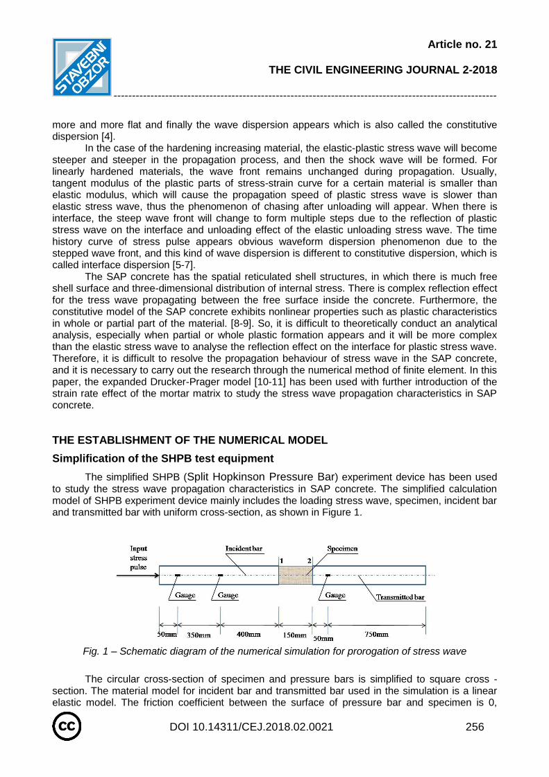
Article no. 21


--------------------------------------------------------------------------------------------------------

DOI 10.14311/CEJ.2018.02.0021 256

more and more flat and finally the wave dispersion appears which is also called the constitutive dispersion [4].

In the case of the hardening increasing material, the elastic-plastic stress wave will become steeper and steeper in the propagation process, and then the shock wave will be formed. For linearly hardened materials, the wave front remains unchanged during propagation. Usually, tangent modulus of the plastic parts of stress-strain curve for a certain material is smaller than elastic modulus, which will cause the propagation speed of plastic stress wave is slower than elastic stress wave, thus the phenomenon of chasing after unloading will appear. When there is interface, the steep wave front will change to form multiple steps due to the reflection of plastic stress wave on the interface and unloading effect of the elastic unloading stress wave. The time history curve of stress pulse appears obvious waveform dispersion phenomenon due to the stepped wave front, and this kind of wave dispersion is different to constitutive dispersion, which is called interface dispersion [5-7].

The SAP concrete has the spatial reticulated shell structures, in which there is much free shell surface and three-dimensional distribution of internal stress. There is complex reflection effect for the tress wave propagating between the free surface inside the concrete. Furthermore, the constitutive model of the SAP concrete exhibits nonlinear properties such as plastic characteristics in whole or partial part of the material. [8-9]. So, it is difficult to theoretically conduct an analytical analysis, especially when partial or whole plastic formation appears and it will be more complex than the elastic stress wave to analyse the reflection effect on the interface for plastic stress wave. Therefore, it is difficult to resolve the propagation behaviour of stress wave in the SAP concrete, and it is necessary to carry out the research through the numerical method of finite element. In this paper, the expanded Drucker-Prager model [10-11] has been used with further introduction of the strain rate effect of the mortar matrix to study the stress wave propagation characteristics in SAP concrete.

THE ESTABLISHMENT OF THE NUMERICAL MODEL

Simplification of the SHPB test equipment

The simplified SHPB (Split Hopkinson Pressure Bar) experiment device has been used to study the stress wave propagation characteristics in SAP concrete. The simplified calculation model of SHPB experiment device mainly includes the loading stress wave, specimen, incident bar and transmitted bar with uniform cross-section, as shown in Figure 1.

Fig. 1 – Schematic diagram of the numerical simulation for prorogation of stress wave

The circular cross-section of specimen and pressure bars is simplified to square cross -section. The material model for incident bar and transmitted bar used in the simulation is a linear elastic model. The friction coefficient between the surface of pressure bar and specimen is 0,

Article no. 21


--------------------------------------------------------------------------------------------------------

DOI 10.14311/CEJ.2018.02.0021 257

which means the friction effect of the interface is ignored in the calculation. The incident bar and transmitted bar are mainly to load and record the stress wave propagation through the specimen. It is necessary to have a long specimen, thus, a complete stress wave with at least a wave length will exist in the specimen. The length of specimen is set to be 150mm with comprehensive regarding of the complete stress wave propagating in the specimen and calculation cost.

Constitutive model of the mortar matrix

The numerical research conducted in this paper is mainly based on the experimental data of SHPB test of the SAP concrete with different porosities, which is 10%, 20%, 30% and 40% respectively, and under quasi static loading or dynamic loading with three strain rate levels of 70/s, 100/s and 140/s. The corresponding mechanical performance data of the SAP concrete is shown in Table 1.The uniaxial compressive stress-strain curve under quasi static loading of the mortar matrix is shown in Figure 2 (a), and this typical stress-strain curve can be simplified as shown in Figure 2 (b). In the generic numerical simulation software ABAQUS, the expanded Drucker-Prager model can describe the characteristics of the stress-strain relationship shown in Figure 2, and the expanded Drucker - Prager model can also reflect the hydrostatic pressure correlation of the materials.

Tab. 1 - Mechanical properties of SAP concrete subjected to quasi static

and high strain-rate loading

Theoretical porosity (%)

Real porosity (%)

Quasi static strength (MPa)

Average strain rate

(/s)

Compressive strength (MPa)

DIF-fc

10 9.5 53.6

79.7 95.4 1.78

107.6 102.4 1.91

140.2 108.8 2.03

20 19.3 37.9

68.2 68.2 1.80

100.0 74.7 1.97

126.9 80.3 2.12

30 27.8 20.9

70.5 40.1 1.92

104.7 45.1 2.16

142.7 50.8 2.43

40 38.7 15.6

72.1 30.7 1.97

101.5 36.0 2.31

141.5 40.2 2.58

Article no. 21


--------------------------------------------------------------------------------------------------------

DOI 10.14311/CEJ.2018.02.0021 258

(a) Quasi-static uniaxial stress-strain curve of

the mortar matrix (b) Simplified quasi-static uniaxial stress-strain

curve of the mortar matrix Fig. 2 – Quasi-static uniaxial stress-strain curve

The pressure bar used in the numerical model includes three different kinds of materials: mortar matrix of SAP concrete, steel fiber concrete, and corundum concrete. The pressure bar of mortar matrix of SAP concrete is mainly used to study the waveform changes before and after the SAP concrete specimens. The pressure bar of steel fiber concrete and corundum concrete mainly used in protective engineering is to study the influence of multilayer material with SAP concrete middle layer on stress wave propagation. When the material of pressure and specimen are the same, the wave impedance of pressure bar and specimen is equal and it can reduce the reflection of stress wave on the interface, at the same time decrease the stress wave attenuation and dispersion in the pressure bar. The linear elastic model was selected for pressure bar and the density, elastic modulus and Poisson’s ratio were in accordance with the mortar matrix. When pressure bar using steel fiber concrete and corundum concrete, the material model was also the same linear elastic model, material density and elastic modulus obtained from the research before. For the convenience of description, the pressure of mortar matrix, steel fiber reinforced concrete and corundum aggregate concrete were named pressure bar 1, pressure bar 2 and pressure bar 3 respectively. From the pressure bar 1 to 3, the impedance between pressure bar and SAP concrete specimen increases. The expanded Drucker - Prager model was used to describe the SAP concrete specimen, and the model parameters are listed in Table 2.

Tab. 2 - Material properties involved in the numerical model

Material density

(kg/m3)

Elastic modulus

(GPa)

Poisson’s ratio

Compressive strength

(MPa)

Friction angle

Dilatancy angle

K

Pressure bar 1

2172 24.2 0.21 — — — —

Pressure bar 2

2700 47.5 0.18 — — — —

Pressure bar 3

3800 400 0.3 — — — —

Mortar matrix 2172 24.2 0.21 70.5 46° 46° 1

Article no. 21


--------------------------------------------------------------------------------------------------------

DOI 10.14311/CEJ.2018.02.0021 259

The parameters for expanded Drucker - Prager model displayed in Table 2 do not consider the strain rate effect of SAP concrete material itself, which needs to be added to the expanded Drucker - Prager model. The strain rate effect of SAP concrete material itself can be obtained by numerical studying the lateral inertial confinement effect and friction effect in SHPB test of the SAP concrete with different porosities. The formula suggested by CEB [12] can be used to fit the function of the strain rate effect caused by material itself and strain rate, by which the fitting parameters β and γ can be obtained for each porosity. Then, the function of parameter β and γ and porosity can be fitted as:

1.625 0.0568

0.5804

1V

e

(1)

4 21.69 10 0.0134 0.2684V V

(2)

According to the fitting Equation 1 and Equation 2, it can be deduced that parameters β=0.095, γ=0.268 when the porosity is equal to zero, namely this parameter value of β and γ represent the strain rate effect at high strain rates of mortar matrix caused by the material itself. Thus, the variation of dynamic compressive strength increment caused by materials itself of the mortar matrix and strain rate can be obtained as the equation recommended by CEB:

1.026

0.095

( / ) 30 /

0.268( / ) 30 /

s

sc

c

css

sfDIF f

f s

(3)

The dynamic mechanical behaviour of SAP concrete can be simulated by introduction of the Equation 3 into expanded Drucker - Prager model. However, the Equation 3 may contain some errors coming from the experiment, data processing and numerical model. The strain rate effect parameters β and γ=0.268 for mortar matrix need to be adjusted, based on the stress-strain curves in SHPB test, through trial calculation in order to accurately obtain the stress wave propagation law for SAP concrete with different porosities. The strain rate effect parameters β and γ=0.268 for mortar matrix after calibration are shown in Table 3.

Tab. 3 - Parameter β and γ of the matrix

Porosity of the specimen (%) β γ

10 1.03 2.38

20 1.12 2.22

30 1.19 2.13

40 1.25 1.97

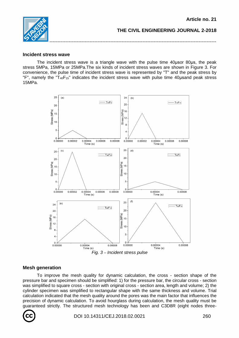
Article no. 21


--------------------------------------------------------------------------------------------------------

DOI 10.14311/CEJ.2018.02.0021 260

Incident stress wave

The incident stress wave is a triangle wave with the pulse time 40μsor 80μs, the peak stress 5MPa, 15MPa or 25MPa.The six kinds of incident stress waves are shown in Figure 3. For convenience, the pulse time of incident stress wave is represented by "T" and the peak stress by "F", namely the "T40F15" indicates the incident stress wave with pulse time 40μsand peak stress 15MPa.

Fig. 3 – Incident stress pulse

Mesh generation

To improve the mesh quality for dynamic calculation, the cross - section shape of the pressure bar and specimen should be simplified: 1) for the pressure bar, the circular cross - section was simplified to square cross - section with original cross - section area, length and volume; 2) the cylinder specimen was simplified to rectangular shape with the same thickness and volume. Trial calculation indicated that the mesh quality around the pores was the main factor that influences the precision of dynamic calculation. To avoid hourglass during calculation, the mesh quality must be guaranteed strictly. The structured mesh technology has been and C3D8R (eight nodes three-

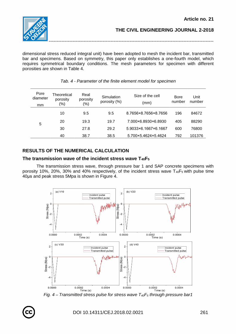
Article no. 21


--------------------------------------------------------------------------------------------------------

DOI 10.14311/CEJ.2018.02.0021 261

dimensional stress reduced integral unit) have been adopted to mesh the incident bar, transmitted bar and specimens. Based on symmetry, this paper only establishes a one-fourth model, which requires symmetrical boundary conditions. The mesh parameters for specimen with different porosities are shown in Table 4.

Tab. 4 - Parameter of the finite element model for specimen

Pore diameter

mm

Theoretical porosity

(%)

Real porosity

(%)

Simulation porosity (%)

Size of the cell

(mm)

Bore number

Unit number

5

10 9.5 9.5 8.7656×8.7656×8.7656 196 84672

20 19.3 19.7 7.000×6.8930×6.8930 405 88290

30 27.8 29.2 5.9033×6.1667×6.1667 600 76800

40 38.7 38.5 5.700×5.4624×5.4624 792 101376

RESULTS OF THE NUMERICAL CALCULATION

The transmission wave of the incident stress wave T40F5

The transmission stress wave, through pressure bar 1 and SAP concrete specimens with porosity 10%, 20%, 30% and 40% respectively, of the incident stress wave T40F5 with pulse time 40μs and peak stress 5Mpa is shown in Figure 4.

Fig. 4 – Transmitted stress pulse for stress wave T40F5 through pressure bar1

Article no. 21


--------------------------------------------------------------------------------------------------------

DOI 10.14311/CEJ.2018.02.0021 262


The transmission stress wave, through pressure bar 2 and SAP concrete specimens with porosity 10%, 20%, 30% and 40% respectively, of the incident stress wave T40F15 with pulse time 40μs and peak stress 15 MPa is shown in Figure 5.




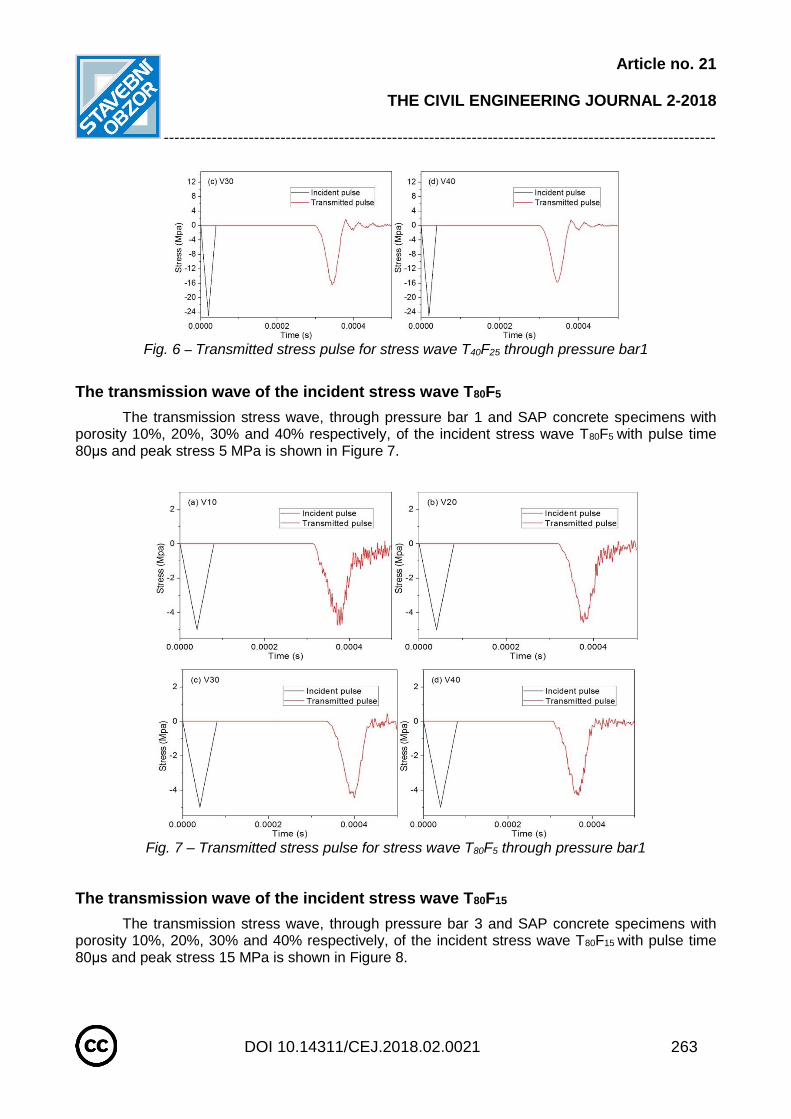
Article no. 21


--------------------------------------------------------------------------------------------------------

DOI 10.14311/CEJ.2018.02.0021 263







Article no. 21


--------------------------------------------------------------------------------------------------------

DOI 10.14311/CEJ.2018.02.0021 264





Article no. 21


--------------------------------------------------------------------------------------------------------

DOI 10.14311/CEJ.2018.02.0021 265

DISCUSSION

The influence of porosity on ratio of transmitted peak stress

Figure 10 shows the ratio of peak stress of transmitted stress wave and incident stress wave (ratio of transmitted peak stress) through pressure bar 1, bar 2 and bar 3 respectively with the change of porosities of specimens. In Figure 10(a) is shown the influence of SAP concrete on stress wave propagation without the influence of impedance matching of different medium. It can be seen from the Figure 10 (a) that: the ratios of transmitted peak stress are all less than 1; the ratios of transmitted peak stress decreases with increase of porosity; the ratios of transmitted peak stress of the incident stress with short pulse time is significantly smaller than that of the incident stress with long pulse time. The SAP concrete has significant attenuation for stress wave, and the attenuation will increase with rise of porosity, while decrease with increase of pulse time. Figure 10 (b) and Figure 10 (c) display the effect of SAP concrete and interface of pressure bar and specimen on propagation property of stress waves considering the impedance mismatch. It can be seen from Figure 10 (b) and Figure 10 (c) that the ratio of transmitted peak stress still increases with the rise of porosity and decrease of pulse time when there exists impedance mismatch.

Fig. 10 – Ratio of transmitted peak stress through pressure bar 1, bar 2 and bar 3 respectively

The influence of wave impedance ratio on ratio of transmitted peak stress

Figure11 shows that the ratios of transmitted peak stress vary with porosity when incident stress wave T40F15 and T80F15propagates into specimen through pressure bar 1, pressure bar 2 and pressure bar 3 respectively. The interface impedance ratio of stress wave λ is 1, 1.56 and 5.38 on the interface of specimen and pressure bar 1, pressure bar 2 and pressure bar 3 respectively.

Article no. 21


--------------------------------------------------------------------------------------------------------

DOI 10.14311/CEJ.2018.02.0021 266

In Figure11 (a) and Figure 11 (b), it can be seen that the ratios of transmitted peak stress decreases with increase of the interface impedance ratio of stress wave λ, especially for the incident stress wave T80F15 with long pulse time the trend is more obvious. The ratio of transmitted peak stress is less than 0.61 and 0.88 for incident stress wave T40F15 and T80F15 respectively when the interface impedance ratio of stress wave λ is equal to 1. When the interface impedance ratio of stress wave λ rises to 5.38, the ratio of transmitted peak stress is less than o.42 and 0.46 for incident stress wave T40F15 and T80F15 respectively. The multilayer materials with SAP concrete as middle layer can greatly improve the attenuation effect of stress wave combined with attenuation effect by SAP concrete itself and adjustment of wave impedance ratio of different materials.

Fig. 11 – Ratio of transmitted peak stress of T40F15 and T80F15 through pressure bar 1, bar, bar 3

The dispersion effect of SAP concrete on the stress wave

As can be seen from Figure 4 to Figure 9, almost all the waveform appear dispersion phenomenon after passing through SAP concrete specimens. The wave dispersion effect includes three aspects: one is that the sharp corners of the triangle wave become smooth and even flat; the second is the rise time of stress waves will be extended; the third effect is that the stress wave oscillates after passing through SAP concrete specimens. The SAP concrete has a large number of free surface of spherical pore. Plastic stress waves can be reflected constantly between the interface and the elastic unloading wave has unloading effect. Thus, multiple steps will occur for the steep loading wave and time history curve of transmitted stress wave will appear obvious dispersion phenomenon because of step wave surface, namely the SAP concrete has significant interface dispersion effect for stress waves.

CONCLUSION

SAP concrete has attenuation function on stress waves. The SAP concrete with higher porosity has greater attenuation effect of stress wave. The attenuation effect will increase with decrease of pulse time of stress wave when given certain porosity for the concrete .The ratio of transmitted peak stress decreases with increase of the interface impedance ratio. The multilayer materials with SAP concrete as middle layer can greatly improve the attenuation effect of stress wave combined with attenuation effect by SAP concrete itself and adjustment of wave impedance ratio of different materials. SAP concrete can cause significant dispersion of stress waves, and the wave dispersion effect includes three aspects: waveform become flat; prolong the rising time; waveform oscillates after passing through SAP concrete specimens. The first two dispersion phenomenon can be attributed to the constitutive dispersion, and the third dispersion phenomenon

Article no. 21


--------------------------------------------------------------------------------------------------------

DOI 10.14311/CEJ.2018.02.0021 267

can be attributed to the interface diffusion. SAP concrete has significant interface dispersion effect for stress waves. Due to the lightweight in nature, energy absorbing and shock attenuation properties of the cellular concrete, which have been investigated in this research, the SAP concrete can be used in road sub-base, airport stopping pads, wall panels and composite sandwich panels.

ACKNOWLEDGEMENTS

We are indebted to the Chinese Natural Science Foundation Project of CQ CSTC (cstc2014jcyjA50026) and the Graduate Student Innovation Fund of Chongqing (CYB16127) for support of this research.

REFERENCES [1] Wang F.Z., Yang J., Cheng H., Wu J., Liang X.Y., 2015. Study on the mechanism of desorption

behavior of saturated SAP in concrete. ACI matererials journal, vol. 112: 463-470

[2] Yang J., Wang F.Z., Liu Y.P., 2015. Comparison of ordinary pores with internal cured pores

produced by superabsorbent polymers. Advanced materials research, 1129: 315-322

[3] Wang F.Z., Yang J., Hu S.G., Li X.P., Cheng H., 2016. Influence of superabsorbent polymers on the

surrounding cement paste. Cement and concrete research, vol. 81: 112-121

[4] Wang L., Wang Y.G., 2005. The important role of stress waves in the study on dynamic constitutive

behavior of materials by SHPB. Explosion and shock waves, vol. 25: 17-25

[5] Godin O.A., Chapman D.M., 2001. Dispersion of interface waves in sediments with power-law

shear speed profiles. I. Exact and approximate analytical results. Journal of the Acoustical society of

america, vol. 110:1890-907

[6] Chapman D.M.F., Godin O.A., 2001. Dispersion of interface waves in sediments with power-law

shear speed profiles. II. Experimental observations and seismo-acoustic inversions. Journal of the acoustical

society of america,vol. 110:1908-16

[7] Murty G.S., 1975. A theoretical model for the attenuation and dispersion of stoneley waves at the

loosely bonded interface of elastic half spaces. Physics of the earth & planetary interiors, vol. 11: 65-79

[8] Deng Z.P., Cheng H., Wang Z.G., Zhu G.H., Zhong H.S., 2016. Compressive behavior of the cellular

concrete utilizing millimeter-size saturated SAP under high strain-rate loading. Construction and building

materials, vol. 119: 96-106

[9] Deng Z.P., Cheng H., Zhu G.H., 2015. Dynamic behavior and constitutive model of super absorbent

polymer concrete under impact loading. International journal of earth sciences and engineering, vol. 8: 2974-

2980

[10] Drucker D.C., Prager W., 1952. Soil mechanics and plastic analysis or limit design. Quarterly of

applied mathematics, vol.10: 157-165

[11] Li Q.M., Meng H., 2003. About the dynamic strength enhancement of concrete-like materials in a

split Hopkinson pressure bar test . Solids and structures, vol. 40: 343-360

[12] Bischoff P.H., Perry S.H., 1991. Compressive behavior of concrete at high strain rate. Materials and

structures, vol. 24: 42-450

javascript:;

http://xueshu.baidu.com/s?wd=author%3A%28Godin%20OA%29%20&tn=SE_baiduxueshu_c1gjeupa&ie=utf-8&sc_f_para=sc_hilight%3Dperson

http://xueshu.baidu.com/s?wd=author%3A%28Godin%20OA%29%20&tn=SE_baiduxueshu_c1gjeupa&ie=utf-8&sc_f_para=sc_hilight%3Dperson

http://xueshu.baidu.com/s?wd=paperuri%3A%28794d53e78db2332d37f27ba95b2c490c%29&filter=sc_long_sign&tn=SE_xueshusource_2kduw22v&sc_vurl=http%3A%2F%2Fwww.ncbi.nlm.nih.gov%2Fpubmed%2F11681370&ie=utf-8&sc_us=14119598784393823604

http://xueshu.baidu.com/s?wd=paperuri%3A%28794d53e78db2332d37f27ba95b2c490c%29&filter=sc_long_sign&tn=SE_xueshusource_2kduw22v&sc_vurl=http%3A%2F%2Fwww.ncbi.nlm.nih.gov%2Fpubmed%2F11681370&ie=utf-8&sc_us=14119598784393823604

http://xueshu.baidu.com/usercenter/data/journal?cmd=jump&wd=journaluri%3A%2836fb6e2356bf9ddf%29%20%E3%80%8AJournal%20of%20the%20Acoustical%20Society%20of%20America%E3%80%8B&tn=SE_baiduxueshu_c1gjeupa&ie=utf-8&sc_f_para=sc_hilight%3Dpublish&sort=sc_cited


http://xueshu.baidu.com/s?wd=author%3A%28David%20M.%20F.%20Chapman%29%20&tn=SE_baiduxueshu_c1gjeupa&ie=utf-8&sc_f_para=sc_hilight%3Dperson

http://xueshu.baidu.com/s?wd=author%3A%28David%20M.%20F.%20Chapman%29%20&tn=SE_baiduxueshu_c1gjeupa&ie=utf-8&sc_f_para=sc_hilight%3Dperson

http://xueshu.baidu.com/s?wd=paperuri%3A%28a45cc34e5ad733322446dadaa7333750%29&filter=sc_long_sign&tn=SE_xueshusource_2kduw22v&sc_vurl=http%3A%2F%2Fscitation.aip.org%2Fcontent%2Fasa%2Fjournal%2Fjasa%2F110%2F4%2F10.1121%2F1.1401739&ie=utf-8&sc_us=17265814982191845351

http://xueshu.baidu.com/s?wd=paperuri%3A%28a45cc34e5ad733322446dadaa7333750%29&filter=sc_long_sign&tn=SE_xueshusource_2kduw22v&sc_vurl=http%3A%2F%2Fscitation.aip.org%2Fcontent%2Fasa%2Fjournal%2Fjasa%2F110%2F4%2F10.1121%2F1.1401739&ie=utf-8&sc_us=17265814982191845351



http://xueshu.baidu.com/s?wd=author%3A%28G.S.%20Murty%29%20&tn=SE_baiduxueshu_c1gjeupa&ie=utf-8&sc_f_para=sc_hilight%3Dperson

http://xueshu.baidu.com/s?wd=paperuri%3A%28d3a06dbf8cf0a6f0630660929ae1d6dd%29&filter=sc_long_sign&tn=SE_xueshusource_2kduw22v&sc_vurl=http%3A%2F%2Fwww.sciencedirect.com%2Fscience%2Farticle%2Fpii%2F003192017590076X&ie=utf-8&sc_us=11571718671632304328

http://xueshu.baidu.com/s?wd=paperuri%3A%28d3a06dbf8cf0a6f0630660929ae1d6dd%29&filter=sc_long_sign&tn=SE_xueshusource_2kduw22v&sc_vurl=http%3A%2F%2Fwww.sciencedirect.com%2Fscience%2Farticle%2Fpii%2F003192017590076X&ie=utf-8&sc_us=11571718671632304328

http://xueshu.baidu.com/usercenter/data/journal?cmd=jump&wd=journaluri%3A%28907237bf7bbcbb18%29%20%E3%80%8APhysics%20of%20the%20Earth%20%26%20Planetary%20Interiors%E3%80%8B&tn=SE_baiduxueshu_c1gjeupa&ie=utf-8&sc_f_para=sc_hilight%3Dpublish&sort=sc_cited

STAVEBNÍ OBZOR - CKAIT

Documents

Transcript of STAVEBNÍ OBZOR - CKAIT