
Statistics Toolbox - Department of Radio Engineering FEE...
560
For Use with MATLAB ® Computation Visualization Programming Statistics Toolbox User’s Guide Version 3
-
Upload
duongtuyen -
Category
Documents
-
view
217 -
download
0
Transcript of Statistics Toolbox - Department of Radio Engineering FEE...

For Use with MATLAB®
Computation
Visualization
Programming
StatisticsToolbox
User’s GuideVersion 3

How to Contact The MathWorks:
508-647-7000 Phone
508-647-7001 Fax
The MathWorks, Inc. Mail3 Apple Hill DriveNatick, MA 01760-2098
http://www.mathworks.com Webftp.mathworks.com Anonymous FTP servercomp.soft-sys.matlab Newsgroup
[email protected] Technical [email protected] Product enhancement [email protected] Bug [email protected] Documentation error [email protected] Subscribing user [email protected] Order status, license renewals, [email protected] Sales, pricing, and general information
Statistics Toolbox User’s Guide COPYRIGHT 1993 - 2000 by The MathWorks, Inc.The software described in this document is furnished under a license agreement. The software may be usedor copied only under the terms of the license agreement. No part of this manual may be photocopied or repro-duced in any form without prior written consent from The MathWorks, Inc.
FEDERAL ACQUISITION: This provision applies to all acquisitions of the Program and Documentation byor for the federal government of the United States. By accepting delivery of the Program, the governmenthereby agrees that this software qualifies as "commercial" computer software within the meaning of FARPart 12.212, DFARS Part 227.7202-1, DFARS Part 227.7202-3, DFARS Part 252.227-7013, and DFARS Part252.227-7014. The terms and conditions of The MathWorks, Inc. Software License Agreement shall pertainto the government’s use and disclosure of the Program and Documentation, and shall supersede anyconflicting contractual terms or conditions. If this license fails to meet the government’s minimum needs oris inconsistent in any respect with federal procurement law, the government agrees to return the Programand Documentation, unused, to MathWorks.
MATLAB, Simulink, Stateflow, Handle Graphics, and Real-Time Workshop are registered trademarks, andTarget Language Compiler is a trademark of The MathWorks, Inc.
Other product or brand names are trademarks or registered trademarks of their respective holders.
Printing History: September 1993 First printing Version 1March 1996 Second printing Version 2January 1997 Third printing For MATLAB 5May 1997 Revised for MATLAB 5.1 (online version)January 1998 Revised for MATLAB 5.2 (online version)January 1999 Revised for Version 2.1.2 (Release 11) (online only)November 2000 Fourth printing Revised for Version 3 (Release 12)

i
Contents
Preface
Overview . . . . . . . . . . . . . . . . . . . . . . . . . . . . . . . . . . . . . . . . . . . . . xii
What Is the Statistics Toolbox? . . . . . . . . . . . . . . . . . . . . . . . . . xiii
How to Use This Guide . . . . . . . . . . . . . . . . . . . . . . . . . . . . . . . . xiv
Related Products List . . . . . . . . . . . . . . . . . . . . . . . . . . . . . . . . . . xv
Mathematical Notation . . . . . . . . . . . . . . . . . . . . . . . . . . . . . . . xvii
Typographical Conventions . . . . . . . . . . . . . . . . . . . . . . . . . . xviii
1Tutorial
Introduction . . . . . . . . . . . . . . . . . . . . . . . . . . . . . . . . . . . . . . . . . 1-2Primary Topic Areas . . . . . . . . . . . . . . . . . . . . . . . . . . . . . . . . . . 1-2
Probability Distributions . . . . . . . . . . . . . . . . . . . . . . . . . . . . . . 1-5Overview of the Functions . . . . . . . . . . . . . . . . . . . . . . . . . . . . . 1-6Overview of the Distributions . . . . . . . . . . . . . . . . . . . . . . . . . . 1-12
Descriptive Statistics . . . . . . . . . . . . . . . . . . . . . . . . . . . . . . . . 1-43Measures of Central Tendency (Location) . . . . . . . . . . . . . . . . 1-43Measures of Dispersion . . . . . . . . . . . . . . . . . . . . . . . . . . . . . . . 1-45Functions for Data with Missing Values (NaNs) . . . . . . . . . . . 1-46Function for Grouped Data . . . . . . . . . . . . . . . . . . . . . . . . . . . . 1-47Percentiles and Graphical Descriptions . . . . . . . . . . . . . . . . . . 1-49The Bootstrap . . . . . . . . . . . . . . . . . . . . . . . . . . . . . . . . . . . . . . 1-50

ii Contents
Cluster Analysis . . . . . . . . . . . . . . . . . . . . . . . . . . . . . . . . . . . . . 1-53Terminology and Basic Procedure . . . . . . . . . . . . . . . . . . . . . . . 1-53Finding the Similarities Between Objects . . . . . . . . . . . . . . . . 1-54Defining the Links Between Objects . . . . . . . . . . . . . . . . . . . . . 1-56Evaluating Cluster Formation . . . . . . . . . . . . . . . . . . . . . . . . . 1-59Creating Clusters . . . . . . . . . . . . . . . . . . . . . . . . . . . . . . . . . . . . 1-64
Linear Models . . . . . . . . . . . . . . . . . . . . . . . . . . . . . . . . . . . . . . . 1-68One-Way Analysis of Variance (ANOVA) . . . . . . . . . . . . . . . . . 1-69Two-Way Analysis of Variance (ANOVA) . . . . . . . . . . . . . . . . . 1-73N-Way Analysis of Variance . . . . . . . . . . . . . . . . . . . . . . . . . . . 1-76Multiple Linear Regression . . . . . . . . . . . . . . . . . . . . . . . . . . . . 1-82Quadratic Response Surface Models . . . . . . . . . . . . . . . . . . . . . 1-86Stepwise Regression . . . . . . . . . . . . . . . . . . . . . . . . . . . . . . . . . 1-88Generalized Linear Models . . . . . . . . . . . . . . . . . . . . . . . . . . . . 1-91Robust and Nonparametric Methods . . . . . . . . . . . . . . . . . . . . 1-95
Nonlinear Regression Models . . . . . . . . . . . . . . . . . . . . . . . . 1-100Example: Nonlinear Modeling . . . . . . . . . . . . . . . . . . . . . . . . . 1-100
Hypothesis Tests . . . . . . . . . . . . . . . . . . . . . . . . . . . . . . . . . . . . 1-105Hypothesis Test Terminology . . . . . . . . . . . . . . . . . . . . . . . . . 1-105Hypothesis Test Assumptions . . . . . . . . . . . . . . . . . . . . . . . . . 1-106Example: Hypothesis Testing . . . . . . . . . . . . . . . . . . . . . . . . . 1-107Available Hypothesis Tests . . . . . . . . . . . . . . . . . . . . . . . . . . . 1-111
Multivariate Statistics . . . . . . . . . . . . . . . . . . . . . . . . . . . . . . . 1-112Principal Components Analysis . . . . . . . . . . . . . . . . . . . . . . . 1-112Multivariate Analysis of Variance (MANOVA) . . . . . . . . . . . 1-122
Statistical Plots . . . . . . . . . . . . . . . . . . . . . . . . . . . . . . . . . . . . . 1-128Box Plots . . . . . . . . . . . . . . . . . . . . . . . . . . . . . . . . . . . . . . . . . . 1-128Distribution Plots . . . . . . . . . . . . . . . . . . . . . . . . . . . . . . . . . . . 1-129Scatter Plots . . . . . . . . . . . . . . . . . . . . . . . . . . . . . . . . . . . . . . . 1-135
Statistical Process Control (SPC) . . . . . . . . . . . . . . . . . . . . . 1-138Control Charts . . . . . . . . . . . . . . . . . . . . . . . . . . . . . . . . . . . . . 1-138Capability Studies . . . . . . . . . . . . . . . . . . . . . . . . . . . . . . . . . . 1-141

iii
Design of Experiments (DOE) . . . . . . . . . . . . . . . . . . . . . . . . 1-143Full Factorial Designs . . . . . . . . . . . . . . . . . . . . . . . . . . . . . . . 1-144Fractional Factorial Designs . . . . . . . . . . . . . . . . . . . . . . . . . . 1-145D-Optimal Designs . . . . . . . . . . . . . . . . . . . . . . . . . . . . . . . . . . 1-147
Demos . . . . . . . . . . . . . . . . . . . . . . . . . . . . . . . . . . . . . . . . . . . . . 1-153The disttool Demo . . . . . . . . . . . . . . . . . . . . . . . . . . . . . . . . . . 1-154The polytool Demo . . . . . . . . . . . . . . . . . . . . . . . . . . . . . . . . . . 1-156The aoctool Demo . . . . . . . . . . . . . . . . . . . . . . . . . . . . . . . . . . . 1-161The randtool Demo . . . . . . . . . . . . . . . . . . . . . . . . . . . . . . . . . . 1-169The rsmdemo Demo . . . . . . . . . . . . . . . . . . . . . . . . . . . . . . . . 1-170The glmdemo Demo . . . . . . . . . . . . . . . . . . . . . . . . . . . . . . . . . 1-172The robustdemo Demo . . . . . . . . . . . . . . . . . . . . . . . . . . . . . . . 1-172
Selected Bibliography . . . . . . . . . . . . . . . . . . . . . . . . . . . . . . . 1-175
2Reference
Function Category List . . . . . . . . . . . . . . . . . . . . . . . . . . . . . . . . 2-3anova1 . . . . . . . . . . . . . . . . . . . . . . . . . . . . . . . . . . . . . . . . . . . . . 2-17anova2 . . . . . . . . . . . . . . . . . . . . . . . . . . . . . . . . . . . . . . . . . . . . . 2-23anovan . . . . . . . . . . . . . . . . . . . . . . . . . . . . . . . . . . . . . . . . . . . . 2-27aoctool . . . . . . . . . . . . . . . . . . . . . . . . . . . . . . . . . . . . . . . . . . . . . 2-33barttest . . . . . . . . . . . . . . . . . . . . . . . . . . . . . . . . . . . . . . . . . . . . 2-36betacdf . . . . . . . . . . . . . . . . . . . . . . . . . . . . . . . . . . . . . . . . . . . . . 2-37betafit . . . . . . . . . . . . . . . . . . . . . . . . . . . . . . . . . . . . . . . . . . . . . 2-38betainv . . . . . . . . . . . . . . . . . . . . . . . . . . . . . . . . . . . . . . . . . . . . 2-40betalike . . . . . . . . . . . . . . . . . . . . . . . . . . . . . . . . . . . . . . . . . . . . 2-41betapdf . . . . . . . . . . . . . . . . . . . . . . . . . . . . . . . . . . . . . . . . . . . . 2-42betarnd . . . . . . . . . . . . . . . . . . . . . . . . . . . . . . . . . . . . . . . . . . . . 2-43betastat . . . . . . . . . . . . . . . . . . . . . . . . . . . . . . . . . . . . . . . . . . . . 2-44binocdf . . . . . . . . . . . . . . . . . . . . . . . . . . . . . . . . . . . . . . . . . . . . . 2-45binofit . . . . . . . . . . . . . . . . . . . . . . . . . . . . . . . . . . . . . . . . . . . . . 2-46binoinv . . . . . . . . . . . . . . . . . . . . . . . . . . . . . . . . . . . . . . . . . . . . 2-47binopdf . . . . . . . . . . . . . . . . . . . . . . . . . . . . . . . . . . . . . . . . . . . . 2-48binornd . . . . . . . . . . . . . . . . . . . . . . . . . . . . . . . . . . . . . . . . . . . . 2-49

iv Contents
binostat . . . . . . . . . . . . . . . . . . . . . . . . . . . . . . . . . . . . . . . . . . . . 2-50bootstrp . . . . . . . . . . . . . . . . . . . . . . . . . . . . . . . . . . . . . . . . . . . . 2-51boxplot . . . . . . . . . . . . . . . . . . . . . . . . . . . . . . . . . . . . . . . . . . . . 2-54capable . . . . . . . . . . . . . . . . . . . . . . . . . . . . . . . . . . . . . . . . . . . . 2-56capaplot . . . . . . . . . . . . . . . . . . . . . . . . . . . . . . . . . . . . . . . . . . . . 2-58caseread . . . . . . . . . . . . . . . . . . . . . . . . . . . . . . . . . . . . . . . . . . . 2-60casewrite . . . . . . . . . . . . . . . . . . . . . . . . . . . . . . . . . . . . . . . . . . . 2-61cdf . . . . . . . . . . . . . . . . . . . . . . . . . . . . . . . . . . . . . . . . . . . . . . . . 2-62cdfplot . . . . . . . . . . . . . . . . . . . . . . . . . . . . . . . . . . . . . . . . . . . . . 2-63chi2cdf . . . . . . . . . . . . . . . . . . . . . . . . . . . . . . . . . . . . . . . . . . . . . 2-65chi2inv . . . . . . . . . . . . . . . . . . . . . . . . . . . . . . . . . . . . . . . . . . . . 2-66chi2pdf . . . . . . . . . . . . . . . . . . . . . . . . . . . . . . . . . . . . . . . . . . . . 2-67chi2rnd . . . . . . . . . . . . . . . . . . . . . . . . . . . . . . . . . . . . . . . . . . . . 2-68chi2stat . . . . . . . . . . . . . . . . . . . . . . . . . . . . . . . . . . . . . . . . . . . . 2-69classify . . . . . . . . . . . . . . . . . . . . . . . . . . . . . . . . . . . . . . . . . . . . 2-70cluster . . . . . . . . . . . . . . . . . . . . . . . . . . . . . . . . . . . . . . . . . . . . . 2-71clusterdata . . . . . . . . . . . . . . . . . . . . . . . . . . . . . . . . . . . . . . . . . 2-73combnk . . . . . . . . . . . . . . . . . . . . . . . . . . . . . . . . . . . . . . . . . . . . 2-75cophenet . . . . . . . . . . . . . . . . . . . . . . . . . . . . . . . . . . . . . . . . . . . 2-76cordexch . . . . . . . . . . . . . . . . . . . . . . . . . . . . . . . . . . . . . . . . . . . 2-78corrcoef . . . . . . . . . . . . . . . . . . . . . . . . . . . . . . . . . . . . . . . . . . . . 2-79cov . . . . . . . . . . . . . . . . . . . . . . . . . . . . . . . . . . . . . . . . . . . . . . . . 2-80crosstab . . . . . . . . . . . . . . . . . . . . . . . . . . . . . . . . . . . . . . . . . . . . 2-81daugment . . . . . . . . . . . . . . . . . . . . . . . . . . . . . . . . . . . . . . . . . . 2-83dcovary . . . . . . . . . . . . . . . . . . . . . . . . . . . . . . . . . . . . . . . . . . . . 2-84dendrogram . . . . . . . . . . . . . . . . . . . . . . . . . . . . . . . . . . . . . . . . 2-85disttool . . . . . . . . . . . . . . . . . . . . . . . . . . . . . . . . . . . . . . . . . . . . 2-87dummyvar . . . . . . . . . . . . . . . . . . . . . . . . . . . . . . . . . . . . . . . . . 2-88errorbar . . . . . . . . . . . . . . . . . . . . . . . . . . . . . . . . . . . . . . . . . . . . 2-89ewmaplot . . . . . . . . . . . . . . . . . . . . . . . . . . . . . . . . . . . . . . . . . . 2-90expcdf . . . . . . . . . . . . . . . . . . . . . . . . . . . . . . . . . . . . . . . . . . . . . 2-92expfit . . . . . . . . . . . . . . . . . . . . . . . . . . . . . . . . . . . . . . . . . . . . . . 2-93expinv . . . . . . . . . . . . . . . . . . . . . . . . . . . . . . . . . . . . . . . . . . . . . 2-94exppdf . . . . . . . . . . . . . . . . . . . . . . . . . . . . . . . . . . . . . . . . . . . . . 2-95exprnd . . . . . . . . . . . . . . . . . . . . . . . . . . . . . . . . . . . . . . . . . . . . . 2-96expstat . . . . . . . . . . . . . . . . . . . . . . . . . . . . . . . . . . . . . . . . . . . . 2-97fcdf . . . . . . . . . . . . . . . . . . . . . . . . . . . . . . . . . . . . . . . . . . . . . . . . 2-98ff2n . . . . . . . . . . . . . . . . . . . . . . . . . . . . . . . . . . . . . . . . . . . . . . . 2-99finv . . . . . . . . . . . . . . . . . . . . . . . . . . . . . . . . . . . . . . . . . . . . . . 2-100fpdf . . . . . . . . . . . . . . . . . . . . . . . . . . . . . . . . . . . . . . . . . . . . . . 2-101

v
fracfact . . . . . . . . . . . . . . . . . . . . . . . . . . . . . . . . . . . . . . . . . . . 2-102friedman . . . . . . . . . . . . . . . . . . . . . . . . . . . . . . . . . . . . . . . . . . 2-106frnd . . . . . . . . . . . . . . . . . . . . . . . . . . . . . . . . . . . . . . . . . . . . . . 2-110fstat . . . . . . . . . . . . . . . . . . . . . . . . . . . . . . . . . . . . . . . . . . . . . . 2-111fsurfht . . . . . . . . . . . . . . . . . . . . . . . . . . . . . . . . . . . . . . . . . . . . 2-112fullfact . . . . . . . . . . . . . . . . . . . . . . . . . . . . . . . . . . . . . . . . . . . . 2-114gamcdf . . . . . . . . . . . . . . . . . . . . . . . . . . . . . . . . . . . . . . . . . . . . 2-115gamfit . . . . . . . . . . . . . . . . . . . . . . . . . . . . . . . . . . . . . . . . . . . . 2-116gaminv . . . . . . . . . . . . . . . . . . . . . . . . . . . . . . . . . . . . . . . . . . . 2-117gamlike . . . . . . . . . . . . . . . . . . . . . . . . . . . . . . . . . . . . . . . . . . . 2-118gampdf . . . . . . . . . . . . . . . . . . . . . . . . . . . . . . . . . . . . . . . . . . . 2-119gamrnd . . . . . . . . . . . . . . . . . . . . . . . . . . . . . . . . . . . . . . . . . . . 2-120gamstat . . . . . . . . . . . . . . . . . . . . . . . . . . . . . . . . . . . . . . . . . . . 2-121geocdf . . . . . . . . . . . . . . . . . . . . . . . . . . . . . . . . . . . . . . . . . . . . 2-122geoinv . . . . . . . . . . . . . . . . . . . . . . . . . . . . . . . . . . . . . . . . . . . . 2-123geomean . . . . . . . . . . . . . . . . . . . . . . . . . . . . . . . . . . . . . . . . . . 2-124geopdf . . . . . . . . . . . . . . . . . . . . . . . . . . . . . . . . . . . . . . . . . . . . 2-125geornd . . . . . . . . . . . . . . . . . . . . . . . . . . . . . . . . . . . . . . . . . . . . 2-126geostat . . . . . . . . . . . . . . . . . . . . . . . . . . . . . . . . . . . . . . . . . . . . 2-127gline . . . . . . . . . . . . . . . . . . . . . . . . . . . . . . . . . . . . . . . . . . . . . 2-128glmdemo . . . . . . . . . . . . . . . . . . . . . . . . . . . . . . . . . . . . . . . . . . 2-129glmfit . . . . . . . . . . . . . . . . . . . . . . . . . . . . . . . . . . . . . . . . . . . . . 2-130glmval . . . . . . . . . . . . . . . . . . . . . . . . . . . . . . . . . . . . . . . . . . . . 2-135gname . . . . . . . . . . . . . . . . . . . . . . . . . . . . . . . . . . . . . . . . . . . . 2-137gplotmatrix . . . . . . . . . . . . . . . . . . . . . . . . . . . . . . . . . . . . . . . . 2-139grpstats . . . . . . . . . . . . . . . . . . . . . . . . . . . . . . . . . . . . . . . . . . . 2-142gscatter . . . . . . . . . . . . . . . . . . . . . . . . . . . . . . . . . . . . . . . . . . . 2-143harmmean . . . . . . . . . . . . . . . . . . . . . . . . . . . . . . . . . . . . . . . . 2-145hist . . . . . . . . . . . . . . . . . . . . . . . . . . . . . . . . . . . . . . . . . . . . . . 2-146histfit . . . . . . . . . . . . . . . . . . . . . . . . . . . . . . . . . . . . . . . . . . . . 2-147hougen . . . . . . . . . . . . . . . . . . . . . . . . . . . . . . . . . . . . . . . . . . . 2-148hygecdf . . . . . . . . . . . . . . . . . . . . . . . . . . . . . . . . . . . . . . . . . . . 2-149hygeinv . . . . . . . . . . . . . . . . . . . . . . . . . . . . . . . . . . . . . . . . . . . 2-150hygepdf . . . . . . . . . . . . . . . . . . . . . . . . . . . . . . . . . . . . . . . . . . . 2-151hygernd . . . . . . . . . . . . . . . . . . . . . . . . . . . . . . . . . . . . . . . . . . . 2-152hygestat . . . . . . . . . . . . . . . . . . . . . . . . . . . . . . . . . . . . . . . . . . 2-153icdf . . . . . . . . . . . . . . . . . . . . . . . . . . . . . . . . . . . . . . . . . . . . . . . 2-154inconsistent . . . . . . . . . . . . . . . . . . . . . . . . . . . . . . . . . . . . . . . 2-155iqr . . . . . . . . . . . . . . . . . . . . . . . . . . . . . . . . . . . . . . . . . . . . . . . 2-157jbtest . . . . . . . . . . . . . . . . . . . . . . . . . . . . . . . . . . . . . . . . . . . . . 2-158

vi Contents
kruskalwallis . . . . . . . . . . . . . . . . . . . . . . . . . . . . . . . . . . . . . . 2-160kstest . . . . . . . . . . . . . . . . . . . . . . . . . . . . . . . . . . . . . . . . . . . . . 2-164kstest2 . . . . . . . . . . . . . . . . . . . . . . . . . . . . . . . . . . . . . . . . . . . . 2-169kurtosis . . . . . . . . . . . . . . . . . . . . . . . . . . . . . . . . . . . . . . . . . . . 2-172leverage . . . . . . . . . . . . . . . . . . . . . . . . . . . . . . . . . . . . . . . . . . . 2-174lillietest . . . . . . . . . . . . . . . . . . . . . . . . . . . . . . . . . . . . . . . . . . . 2-175linkage . . . . . . . . . . . . . . . . . . . . . . . . . . . . . . . . . . . . . . . . . . . 2-178logncdf . . . . . . . . . . . . . . . . . . . . . . . . . . . . . . . . . . . . . . . . . . . . 2-181logninv . . . . . . . . . . . . . . . . . . . . . . . . . . . . . . . . . . . . . . . . . . . 2-182lognpdf . . . . . . . . . . . . . . . . . . . . . . . . . . . . . . . . . . . . . . . . . . . 2-184lognrnd . . . . . . . . . . . . . . . . . . . . . . . . . . . . . . . . . . . . . . . . . . . 2-185lognstat . . . . . . . . . . . . . . . . . . . . . . . . . . . . . . . . . . . . . . . . . . . 2-186lsline . . . . . . . . . . . . . . . . . . . . . . . . . . . . . . . . . . . . . . . . . . . . . 2-187mad . . . . . . . . . . . . . . . . . . . . . . . . . . . . . . . . . . . . . . . . . . . . . . 2-188mahal . . . . . . . . . . . . . . . . . . . . . . . . . . . . . . . . . . . . . . . . . . . . 2-189manova1 . . . . . . . . . . . . . . . . . . . . . . . . . . . . . . . . . . . . . . . . . . 2-190manovacluster . . . . . . . . . . . . . . . . . . . . . . . . . . . . . . . . . . . . . 2-194mean . . . . . . . . . . . . . . . . . . . . . . . . . . . . . . . . . . . . . . . . . . . . . 2-196median . . . . . . . . . . . . . . . . . . . . . . . . . . . . . . . . . . . . . . . . . . . 2-197mle . . . . . . . . . . . . . . . . . . . . . . . . . . . . . . . . . . . . . . . . . . . . . . 2-198moment . . . . . . . . . . . . . . . . . . . . . . . . . . . . . . . . . . . . . . . . . . . 2-199multcompare . . . . . . . . . . . . . . . . . . . . . . . . . . . . . . . . . . . . . . . 2-200mvnrnd . . . . . . . . . . . . . . . . . . . . . . . . . . . . . . . . . . . . . . . . . . . 2-207mvtrnd . . . . . . . . . . . . . . . . . . . . . . . . . . . . . . . . . . . . . . . . . . . 2-208nanmax . . . . . . . . . . . . . . . . . . . . . . . . . . . . . . . . . . . . . . . . . . . 2-209nanmean . . . . . . . . . . . . . . . . . . . . . . . . . . . . . . . . . . . . . . . . . . 2-210nanmedian . . . . . . . . . . . . . . . . . . . . . . . . . . . . . . . . . . . . . . . . 2-211nanmin . . . . . . . . . . . . . . . . . . . . . . . . . . . . . . . . . . . . . . . . . . . 2-212nanstd . . . . . . . . . . . . . . . . . . . . . . . . . . . . . . . . . . . . . . . . . . . . 2-213nansum . . . . . . . . . . . . . . . . . . . . . . . . . . . . . . . . . . . . . . . . . . . 2-214nbincdf . . . . . . . . . . . . . . . . . . . . . . . . . . . . . . . . . . . . . . . . . . . 2-215nbininv . . . . . . . . . . . . . . . . . . . . . . . . . . . . . . . . . . . . . . . . . . . 2-216nbinpdf . . . . . . . . . . . . . . . . . . . . . . . . . . . . . . . . . . . . . . . . . . . 2-217nbinrnd . . . . . . . . . . . . . . . . . . . . . . . . . . . . . . . . . . . . . . . . . . . 2-218nbinstat . . . . . . . . . . . . . . . . . . . . . . . . . . . . . . . . . . . . . . . . . . . 2-219ncfcdf . . . . . . . . . . . . . . . . . . . . . . . . . . . . . . . . . . . . . . . . . . . . . 2-220ncfinv . . . . . . . . . . . . . . . . . . . . . . . . . . . . . . . . . . . . . . . . . . . . 2-222ncfpdf . . . . . . . . . . . . . . . . . . . . . . . . . . . . . . . . . . . . . . . . . . . . 2-223ncfrnd . . . . . . . . . . . . . . . . . . . . . . . . . . . . . . . . . . . . . . . . . . . . 2-224ncfstat . . . . . . . . . . . . . . . . . . . . . . . . . . . . . . . . . . . . . . . . . . . . 2-225

vii
nctcdf . . . . . . . . . . . . . . . . . . . . . . . . . . . . . . . . . . . . . . . . . . . . . 2-226nctinv . . . . . . . . . . . . . . . . . . . . . . . . . . . . . . . . . . . . . . . . . . . . 2-227nctpdf . . . . . . . . . . . . . . . . . . . . . . . . . . . . . . . . . . . . . . . . . . . . 2-228nctrnd . . . . . . . . . . . . . . . . . . . . . . . . . . . . . . . . . . . . . . . . . . . . 2-229nctstat . . . . . . . . . . . . . . . . . . . . . . . . . . . . . . . . . . . . . . . . . . . . 2-230ncx2cdf . . . . . . . . . . . . . . . . . . . . . . . . . . . . . . . . . . . . . . . . . . . 2-231ncx2inv . . . . . . . . . . . . . . . . . . . . . . . . . . . . . . . . . . . . . . . . . . . 2-233ncx2pdf . . . . . . . . . . . . . . . . . . . . . . . . . . . . . . . . . . . . . . . . . . . 2-234ncx2rnd . . . . . . . . . . . . . . . . . . . . . . . . . . . . . . . . . . . . . . . . . . . 2-235ncx2stat . . . . . . . . . . . . . . . . . . . . . . . . . . . . . . . . . . . . . . . . . . 2-236nlinfit . . . . . . . . . . . . . . . . . . . . . . . . . . . . . . . . . . . . . . . . . . . . 2-237nlintool . . . . . . . . . . . . . . . . . . . . . . . . . . . . . . . . . . . . . . . . . . . 2-238nlparci . . . . . . . . . . . . . . . . . . . . . . . . . . . . . . . . . . . . . . . . . . . . 2-239nlpredci . . . . . . . . . . . . . . . . . . . . . . . . . . . . . . . . . . . . . . . . . . . 2-240normcdf . . . . . . . . . . . . . . . . . . . . . . . . . . . . . . . . . . . . . . . . . . . 2-242normfit . . . . . . . . . . . . . . . . . . . . . . . . . . . . . . . . . . . . . . . . . . . 2-243norminv . . . . . . . . . . . . . . . . . . . . . . . . . . . . . . . . . . . . . . . . . . . 2-244normpdf . . . . . . . . . . . . . . . . . . . . . . . . . . . . . . . . . . . . . . . . . . 2-245normplot . . . . . . . . . . . . . . . . . . . . . . . . . . . . . . . . . . . . . . . . . . 2-246normrnd . . . . . . . . . . . . . . . . . . . . . . . . . . . . . . . . . . . . . . . . . . 2-248normspec . . . . . . . . . . . . . . . . . . . . . . . . . . . . . . . . . . . . . . . . . . 2-249normstat . . . . . . . . . . . . . . . . . . . . . . . . . . . . . . . . . . . . . . . . . . 2-250pareto . . . . . . . . . . . . . . . . . . . . . . . . . . . . . . . . . . . . . . . . . . . . 2-251pcacov . . . . . . . . . . . . . . . . . . . . . . . . . . . . . . . . . . . . . . . . . . . . 2-252pcares . . . . . . . . . . . . . . . . . . . . . . . . . . . . . . . . . . . . . . . . . . . . 2-253pdf . . . . . . . . . . . . . . . . . . . . . . . . . . . . . . . . . . . . . . . . . . . . . . . 2-254pdist . . . . . . . . . . . . . . . . . . . . . . . . . . . . . . . . . . . . . . . . . . . . . 2-255perms . . . . . . . . . . . . . . . . . . . . . . . . . . . . . . . . . . . . . . . . . . . . 2-258poisscdf . . . . . . . . . . . . . . . . . . . . . . . . . . . . . . . . . . . . . . . . . . . 2-259poissfit . . . . . . . . . . . . . . . . . . . . . . . . . . . . . . . . . . . . . . . . . . . . 2-261poissinv . . . . . . . . . . . . . . . . . . . . . . . . . . . . . . . . . . . . . . . . . . . 2-262poisspdf . . . . . . . . . . . . . . . . . . . . . . . . . . . . . . . . . . . . . . . . . . . 2-263poissrnd . . . . . . . . . . . . . . . . . . . . . . . . . . . . . . . . . . . . . . . . . . 2-264poisstat . . . . . . . . . . . . . . . . . . . . . . . . . . . . . . . . . . . . . . . . . . . 2-265polyconf . . . . . . . . . . . . . . . . . . . . . . . . . . . . . . . . . . . . . . . . . . . 2-266polyfit . . . . . . . . . . . . . . . . . . . . . . . . . . . . . . . . . . . . . . . . . . . . 2-267polytool . . . . . . . . . . . . . . . . . . . . . . . . . . . . . . . . . . . . . . . . . . . 2-268polyval . . . . . . . . . . . . . . . . . . . . . . . . . . . . . . . . . . . . . . . . . . . . 2-269prctile . . . . . . . . . . . . . . . . . . . . . . . . . . . . . . . . . . . . . . . . . . . . 2-270princomp . . . . . . . . . . . . . . . . . . . . . . . . . . . . . . . . . . . . . . . . . . 2-271

viii Contents
qqplot . . . . . . . . . . . . . . . . . . . . . . . . . . . . . . . . . . . . . . . . . . . . 2-272random . . . . . . . . . . . . . . . . . . . . . . . . . . . . . . . . . . . . . . . . . . . 2-274randtool . . . . . . . . . . . . . . . . . . . . . . . . . . . . . . . . . . . . . . . . . . . 2-275range . . . . . . . . . . . . . . . . . . . . . . . . . . . . . . . . . . . . . . . . . . . . . 2-276ranksum . . . . . . . . . . . . . . . . . . . . . . . . . . . . . . . . . . . . . . . . . . 2-277raylcdf . . . . . . . . . . . . . . . . . . . . . . . . . . . . . . . . . . . . . . . . . . . . 2-278raylinv . . . . . . . . . . . . . . . . . . . . . . . . . . . . . . . . . . . . . . . . . . . . 2-279raylpdf . . . . . . . . . . . . . . . . . . . . . . . . . . . . . . . . . . . . . . . . . . . . 2-280raylrnd . . . . . . . . . . . . . . . . . . . . . . . . . . . . . . . . . . . . . . . . . . . 2-281raylstat . . . . . . . . . . . . . . . . . . . . . . . . . . . . . . . . . . . . . . . . . . . 2-282rcoplot . . . . . . . . . . . . . . . . . . . . . . . . . . . . . . . . . . . . . . . . . . . . 2-283refcurve . . . . . . . . . . . . . . . . . . . . . . . . . . . . . . . . . . . . . . . . . . . 2-284refline . . . . . . . . . . . . . . . . . . . . . . . . . . . . . . . . . . . . . . . . . . . . 2-285regress . . . . . . . . . . . . . . . . . . . . . . . . . . . . . . . . . . . . . . . . . . . . 2-286regstats . . . . . . . . . . . . . . . . . . . . . . . . . . . . . . . . . . . . . . . . . . . 2-288ridge . . . . . . . . . . . . . . . . . . . . . . . . . . . . . . . . . . . . . . . . . . . . . 2-290robustdemo . . . . . . . . . . . . . . . . . . . . . . . . . . . . . . . . . . . . . . . . 2-292robustfit . . . . . . . . . . . . . . . . . . . . . . . . . . . . . . . . . . . . . . . . . . 2-293rowexch . . . . . . . . . . . . . . . . . . . . . . . . . . . . . . . . . . . . . . . . . . . 2-297rsmdemo . . . . . . . . . . . . . . . . . . . . . . . . . . . . . . . . . . . . . . . . . . 2-298rstool . . . . . . . . . . . . . . . . . . . . . . . . . . . . . . . . . . . . . . . . . . . . . 2-299schart . . . . . . . . . . . . . . . . . . . . . . . . . . . . . . . . . . . . . . . . . . . . 2-300signrank . . . . . . . . . . . . . . . . . . . . . . . . . . . . . . . . . . . . . . . . . . 2-302signtest . . . . . . . . . . . . . . . . . . . . . . . . . . . . . . . . . . . . . . . . . . . 2-304skewness . . . . . . . . . . . . . . . . . . . . . . . . . . . . . . . . . . . . . . . . . . 2-306squareform . . . . . . . . . . . . . . . . . . . . . . . . . . . . . . . . . . . . . . . . 2-308std . . . . . . . . . . . . . . . . . . . . . . . . . . . . . . . . . . . . . . . . . . . . . . . 2-309stepwise . . . . . . . . . . . . . . . . . . . . . . . . . . . . . . . . . . . . . . . . . . 2-310surfht . . . . . . . . . . . . . . . . . . . . . . . . . . . . . . . . . . . . . . . . . . . . 2-311tabulate . . . . . . . . . . . . . . . . . . . . . . . . . . . . . . . . . . . . . . . . . . . 2-312tblread . . . . . . . . . . . . . . . . . . . . . . . . . . . . . . . . . . . . . . . . . . . . 2-313tblwrite . . . . . . . . . . . . . . . . . . . . . . . . . . . . . . . . . . . . . . . . . . . 2-315tcdf . . . . . . . . . . . . . . . . . . . . . . . . . . . . . . . . . . . . . . . . . . . . . . 2-316tdfread . . . . . . . . . . . . . . . . . . . . . . . . . . . . . . . . . . . . . . . . . . . 2-317tinv . . . . . . . . . . . . . . . . . . . . . . . . . . . . . . . . . . . . . . . . . . . . . . 2-319tpdf . . . . . . . . . . . . . . . . . . . . . . . . . . . . . . . . . . . . . . . . . . . . . . 2-320trimmean . . . . . . . . . . . . . . . . . . . . . . . . . . . . . . . . . . . . . . . . . 2-321trnd . . . . . . . . . . . . . . . . . . . . . . . . . . . . . . . . . . . . . . . . . . . . . . 2-322tstat . . . . . . . . . . . . . . . . . . . . . . . . . . . . . . . . . . . . . . . . . . . . . . 2-323ttest . . . . . . . . . . . . . . . . . . . . . . . . . . . . . . . . . . . . . . . . . . . . . . 2-324

ix
ttest2 . . . . . . . . . . . . . . . . . . . . . . . . . . . . . . . . . . . . . . . . . . . . . 2-326unidcdf . . . . . . . . . . . . . . . . . . . . . . . . . . . . . . . . . . . . . . . . . . . 2-328unidinv . . . . . . . . . . . . . . . . . . . . . . . . . . . . . . . . . . . . . . . . . . . 2-329unidpdf . . . . . . . . . . . . . . . . . . . . . . . . . . . . . . . . . . . . . . . . . . . 2-330unidrnd . . . . . . . . . . . . . . . . . . . . . . . . . . . . . . . . . . . . . . . . . . . 2-331unidstat . . . . . . . . . . . . . . . . . . . . . . . . . . . . . . . . . . . . . . . . . . . 2-332unifcdf . . . . . . . . . . . . . . . . . . . . . . . . . . . . . . . . . . . . . . . . . . . . 2-333unifinv . . . . . . . . . . . . . . . . . . . . . . . . . . . . . . . . . . . . . . . . . . . . 2-334unifit . . . . . . . . . . . . . . . . . . . . . . . . . . . . . . . . . . . . . . . . . . . . . 2-335unifpdf . . . . . . . . . . . . . . . . . . . . . . . . . . . . . . . . . . . . . . . . . . . . 2-336unifrnd . . . . . . . . . . . . . . . . . . . . . . . . . . . . . . . . . . . . . . . . . . . 2-337unifstat . . . . . . . . . . . . . . . . . . . . . . . . . . . . . . . . . . . . . . . . . . . 2-338var . . . . . . . . . . . . . . . . . . . . . . . . . . . . . . . . . . . . . . . . . . . . . . . 2-339weibcdf . . . . . . . . . . . . . . . . . . . . . . . . . . . . . . . . . . . . . . . . . . . 2-341weibfit . . . . . . . . . . . . . . . . . . . . . . . . . . . . . . . . . . . . . . . . . . . . 2-342weibinv . . . . . . . . . . . . . . . . . . . . . . . . . . . . . . . . . . . . . . . . . . . 2-343weiblike . . . . . . . . . . . . . . . . . . . . . . . . . . . . . . . . . . . . . . . . . . . 2-344weibpdf . . . . . . . . . . . . . . . . . . . . . . . . . . . . . . . . . . . . . . . . . . . 2-345weibplot . . . . . . . . . . . . . . . . . . . . . . . . . . . . . . . . . . . . . . . . . . 2-346weibrnd . . . . . . . . . . . . . . . . . . . . . . . . . . . . . . . . . . . . . . . . . . . 2-347weibstat . . . . . . . . . . . . . . . . . . . . . . . . . . . . . . . . . . . . . . . . . . 2-348x2fx . . . . . . . . . . . . . . . . . . . . . . . . . . . . . . . . . . . . . . . . . . . . . . 2-349xbarplot . . . . . . . . . . . . . . . . . . . . . . . . . . . . . . . . . . . . . . . . . . . 2-350zscore . . . . . . . . . . . . . . . . . . . . . . . . . . . . . . . . . . . . . . . . . . . . 2-353ztest . . . . . . . . . . . . . . . . . . . . . . . . . . . . . . . . . . . . . . . . . . . . . . 2-354

x Contents
Preface
Overview . . . . . . . . . . . . . . . . . . . . . xii
What Is the Statistics Toolbox? . . . . . . . . . . . xiii
How to Use This Guide . . . . . . . . . . . . . . . xiv
Related Products List . . . . . . . . . . . . . . . . xv
Mathematical Notation . . . . . . . . . . . . . . . xvii
Typographical Conventions . . . . . . . . . . . . . xviii
Preface
xii
OverviewThis chapter introduces the Statistics Toolbox, and explains how to use thedocumentation. It contains the following sections:
• “What Is the Statistics Toolbox?”
• “How to Use This Guide”
• “Related Products List”
• “Mathematical Notation”
• “Typographical Conventions”

What Is the Statistics Toolbox?
xiii
What Is the Statistics Toolbox?The Statistics Toolbox is a collection of tools built on the MATLAB numericcomputing environment. The toolbox supports a wide range of commonstatistical tasks, from random number generation, to curve fitting, to design ofexperiments and statistical process control. The toolbox provides twocategories of tools:
• Building-block probability and statistics functions
• Graphical, interactive tools
The first category of tools is made up of functions that you can call from thecommand line or from your own applications. Many of these functions areMATLAB M-files, series of MATLAB statements that implement specializedstatistics algorithms. You can view the MATLAB code for these functions usingthe statement
type function_name
You can change the way any toolbox function works by copying and renamingthe M-file, then modifying your copy. You can also extend the toolbox by addingyour own M-files.
Secondly, the toolbox provides a number of interactive tools that let you accessmany of the functions through a graphical user interface (GUI). Together, theGUI-based tools provide an environment for polynomial fitting and prediction,as well as probability function exploration.

Preface
xiv
How to Use This GuideIf you are a new user begin with Chapter 1, “Tutorial.” This chapterintroduces the MATLAB statistics environment through the toolbox functions.It describes the functions with regard to particular areas of interest, such asprobability distributions, linear and nonlinear models, principal componentsanalysis, design of experiments, statistical process control, and descriptivestatistics.
All toolbox users should use Chapter 2, “Reference,” for information aboutspecific tools. For functions, reference descriptions include a synopsis of thefunction’s syntax, as well as a complete explanation of options and operation.Many reference descriptions also include examples, a description of thefunction’s algorithm, and references to additional reading material.
Use this guide in conjunction with the software to learn about the powerfulfeatures that MATLAB provides. Each chapter provides numerous examplesthat apply the toolbox to representative statistical tasks.
The random number generation functions for various probability distributionsare based on all the primitive functions, randn and rand. There are manyexamples that start by generating data using random numbers. To duplicatethe results in these examples, first execute the commands below.
seed = 931316785;rand('seed',seed);randn('seed',seed);
You might want to save these commands in an M-file script called init.m.Then, instead of three separate commands, you need only type init.

Related Products List
xv
Related Products ListThe MathWorks provides several products that are especially relevant to thekinds of tasks you can perform with the Statistics Toolbox.
For more information about any of these products, see either:
• The online documentation for that product if it is installed or if you arereading the documentation from the CD
• The MathWorks Web site, at http://www.mathworks.com; see the “products”section
Note The toolboxes listed below all include functions that extend MATLAB’scapabilities. The blocksets all include blocks that extend Simulink’scapabilities.
Product Description
Data Acquisition Toolbox MATLAB functions for direct access to live,measured data from MATLAB
Database Toolbox Tool for connecting to, and interacting with,most ODBC/JDBC databases from withinMATLAB
Financial Time SeriesToolbox
Tool for analyzing time series data in thefinancial markets
GARCH Toolbox MATLAB functions for univariate GeneralizedAutoregressive Conditional Heteroskedasticity(GARCH) volatility modeling
Image ProcessingToolbox
Complete suite of digital image processing andanalysis tools for MATLAB
Mapping Toolbox Tool for analyzing and displayinggeographically based information from withinMATLAB

Preface
xvi
Neural Network Toolbox Comprehensive environment for neuralnetwork research, design, and simulationwithin MATLAB
Optimization Toolbox Tool for general and large-scale optimization ofnonlinear problems, as well as for linearprogramming, quadratic programming,nonlinear least squares, and solving nonlinearequations
Signal ProcessingToolbox
Tool for algorithm development, signal andlinear system analysis, and time-series datamodeling
System IdentificationToolbox
Tool for building accurate, simplified models ofcomplex systems from noisy time-series data
Product Description
Mathematical Notation
xvii
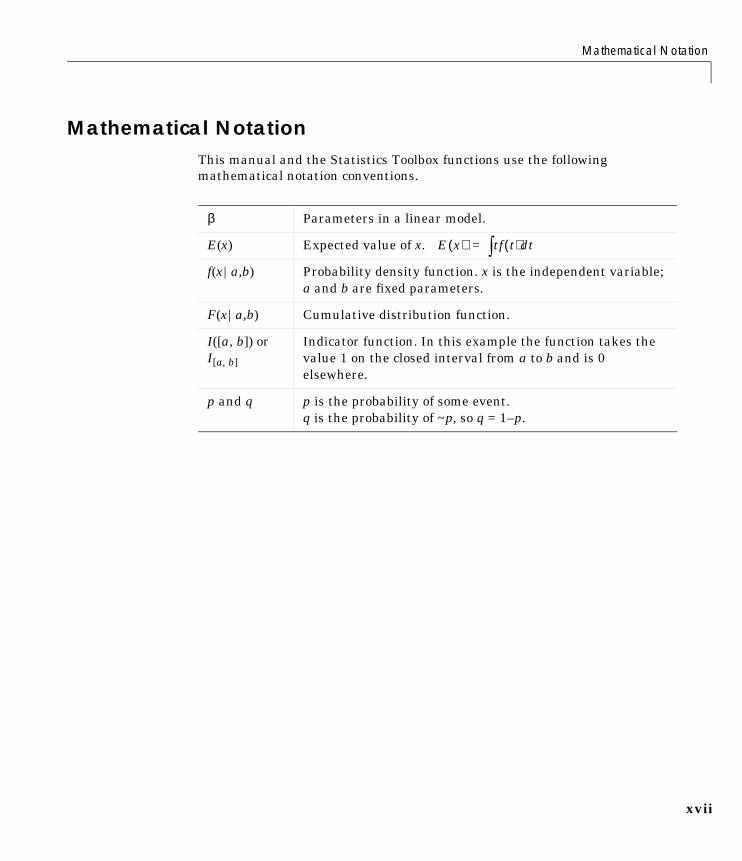
Mathematical NotationThis manual and the Statistics Toolbox functions use the followingmathematical notation conventions.
β Parameters in a linear model.
E(x) Expected value of x.
f(x|a,b) Probability density function. x is the independent variable;a and b are fixed parameters.
F(x|a,b) Cumulative distribution function.
I([a, b]) orI[a, b]
Indicator function. In this example the function takes thevalue 1 on the closed interval from a to b and is 0elsewhere.
p and q p is the probability of some event.q is the probability of ~p, so q = 1–p.
E x( ) tf t( ) td�=

Preface
xviii
Typographical ConventionsThis manual uses some or all of these conventions.
Item Convention to Use Example
Example code Monospace font To assign the value 5 to A,enter
A = 5
Function names/syntax Monospace font The cos function finds thecosine of each array element.
Syntax line example is
MLGetVar ML_var_name
Keys Boldface with an initialcapital letter
Press the Return key.
Literal strings (in syntaxdescriptions in referencechapters)
Monospace bold forliterals
f = freqspace(n,'whole')
Mathematicalexpressions
Italics for variables
Standard text font forfunctions, operators, andconstants
This vector represents thepolynomial
p = x2 + 2x + 3
MATLAB output Monospace font MATLAB responds with
A = 5
Menu names, menu items, andcontrols
Boldface with an initialcapital letter
Choose the File menu.
New terms Italics An array is an orderedcollection of information.
String variables (from a finitelist)
Monospace italics sysc = d2c(sysd,'method')
1
Tutorial
Introduction . . . . . . . . . . . . . . . . . . . . 1-2
Probability Distributions . . . . . . . . . . . . . . 1-5
Descriptive Statistics . . . . . . . . . . . . . . . . 1-43
Cluster Analysis . . . . . . . . . . . . . . . . . . 1-53
Linear Models . . . . . . . . . . . . . . . . . . . 1-68
Nonlinear Regression Models . . . . . . . . . . . 1-100
Hypothesis Tests . . . . . . . . . . . . . . . . . 1-105
Multivariate Statistics . . . . . . . . . . . . . . 1-112
Statistical Plots . . . . . . . . . . . . . . . . . 1-128
Statistical Process Control (SPC) . . . . . . . . . 1-138
Design of Experiments (DOE) . . . . . . . . . . . 1-143
Demos . . . . . . . . . . . . . . . . . . . . . . 1-153
Selected Bibliography . . . . . . . . . . . . . . 1-175

1 Tutorial
1-2
IntroductionThe Statistics Toolbox, for use with MATLAB, supplies basic statisticscapability on the level of a first course in engineering or scientific statistics.The statistics functions it provides are building blocks suitable for use insideother analytical tools.
Primary Topic AreasThe Statistics Toolbox has more than 200 M-files, supporting work in thetopical areas below:
• Probability distributions
• Descriptive statistics
• Cluster analysis
• Linear models
• Nonlinear models
• Hypothesis tests
• Multivariate statistics
• Statistical plots
• Statistical process control
• Design of experiments
Probability DistributionsThe Statistics Toolbox supports 20 probability distributions. For eachdistribution there are five associated functions. They are:
• Probability density function (pdf)
• Cumulative distribution function (cdf)
• Inverse of the cumulative distribution function
• Random number generator
• Mean and variance as a function of the parameters
For data-driven distributions (beta, binomial, exponential, gamma, normal,Poisson, uniform, and Weibull), the Statistics Toolbox has functions forcomputing parameter estimates and confidence intervals.

Introduction
1-3
Descriptive StatisticsThe Statistics Toolbox provides functions for describing the features of a datasample. These descriptive statistics include measures of location and spread,percentile estimates and functions for dealing with data having missingvalues.
Cluster AnalysisThe Statistics Toolbox provides functions that allow you to divide a set ofobjects into subgroups, each having members that are as much alike aspossible. This process is called cluster analysis.
Linear ModelsIn the area of linear models, the Statistics Toolbox supports one-way, two-way,and higher-way analysis of variance (ANOVA), analysis of covariance(ANOCOVA), multiple linear regression, stepwise regression, response surfaceprediction, ridge regression, and one-way multivariate analysis of variance(MANOVA). It supports nonparametric versions of one- and two-way ANOVA.It also supports multiple comparisons of the estimates produced by ANOVAand ANOCOVA functions.
Nonlinear ModelsFor nonlinear models, the Statistics Toolbox provides functions for parameterestimation, interactive prediction and visualization of multidimensionalnonlinear fits, and confidence intervals for parameters and predicted values.
Hypothesis TestsThe Statistics Toolbox also provides functions that do the most common testsof hypothesis – t-tests, Z-tests, nonparametric tests, and distribution tests.
Multivariate StatisticsThe Statistics Toolbox supports methods in multivariate statistics, includingprincipal components analysis, linear discriminant analysis, and one-waymultivariate analysis of variance.

1 Tutorial
1-4
Statistical PlotsThe Statistics Toolbox adds box plots, normal probability plots, Weibullprobability plots, control charts, and quantile-quantile plots to the arsenal ofgraphs in MATLAB. There is also extended support for polynomial curve fittingand prediction. There are functions to create scatter plots or matrices of scatterplots for grouped data, and to identify points interactively on such plots. Thereis a function to interactively explore a fitted regression model.
Statistical Process Control (SPC)For SPC, the Statistics Toolbox provides functions for plotting common controlcharts and performing process capability studies.
Design of Experiments (DOE)The Statistics Toolbox supports full and fractional factorial designs andD-optimal designs. There are functions for generating designs, augmentingdesigns, and optimally assigning units with fixed covariates.

Probability Distributions
1-5
Probability DistributionsProbability distributions arise from experiments where the outcome is subjectto chance. The nature of the experiment dictates which probabilitydistributions may be appropriate for modeling the resulting random outcomes.There are two types of probability distributions – continuous and discrete.
Suppose you are studying a machine that produces videotape. One measure ofthe quality of the tape is the number of visual defects per hundred feet of tape.The result of this experiment is an integer, since you cannot observe 1.5defects. To model this experiment you should use a discrete probabilitydistribution.
A measure affecting the cost and quality of videotape is its thickness. Thicktape is more expensive to produce, while variation in the thickness of the tapeon the reel increases the likelihood of breakage. Suppose you measure thethickness of the tape every 1000 feet. The resulting numbers can take acontinuum of possible values, which suggests using a continuous probabilitydistribution to model the results.
Using a probability model does not allow you to predict the result of anyindividual experiment but you can determine the probability that a givenoutcome will fall inside a specific range of values.
Continuous (data) Continuous (statistics) Discrete
Beta Chi-square Binomial
Exponential Noncentral Chi-square Discrete Uniform
Gamma F Geometric
Lognormal Noncentral F Hypergeometric
Normal t Negative Binomial
Rayleigh Noncentral t Poisson
Uniform
Weibull
1 Tutorial
1-6
This following two sections provide more information about the availabledistributions:
• “Overview of the Functions”
• “Overview of the Distributions”
Overview of the FunctionsMATLAB provides five functions for each distribution, which are discussed inthe following sections:
• “Probability Density Function (pdf)”
• “Cumulative Distribution Function (cdf)”
• “Inverse Cumulative Distribution Function”
• “Random Number Generator”
• “Mean and Variance as a Function of Parameters”
Probability Density Function (pdf)The probability density function (pdf) has a different meaning depending onwhether the distribution is discrete or continuous.
For discrete distributions, the pdf is the probability of observing a particularoutcome. In our videotape example, the probability that there is exactly onedefect in a given hundred feet of tape is the value of the pdf at 1.
Unlike discrete distributions, the pdf of a continuous distribution at a value isnot the probability of observing that value. For continuous distributions theprobability of observing any particular value is zero. To get probabilities youmust integrate the pdf over an interval of interest. For example the probabilityof the thickness of a videotape being between one and two millimeters is theintegral of the appropriate pdf from one to two.
A pdf has two theoretical properties:
• The pdf is zero or positive for every possible outcome.
• The integral of a pdf over its entire range of values is one.
A pdf is not a single function. Rather a pdf is a family of functions characterizedby one or more parameters. Once you choose (or estimate) the parameters of apdf, you have uniquely specified the function.

Probability Distributions
1-7
The pdf function call has the same general format for every distribution in theStatistics Toolbox. The following commands illustrate how to call the pdf forthe normal distribution.
x = [-3:0.1:3];f = normpdf(x,0,1);
The variable f contains the density of the normal pdf with parameters µ=0 andσ=1 at the values in x. The first input argument of every pdf is the set of valuesfor which you want to evaluate the density. Other arguments contain as manyparameters as are necessary to define the distribution uniquely. The normaldistribution requires two parameters; a location parameter (the mean, µ) anda scale parameter (the standard deviation, σ).
Cumulative Distribution Function (cdf)If f is a probability density function for random variable X, the associatedcumulative distribution function (cdf) F is
The cdf of a value x, F(x), is the probability of observing any outcome less thanor equal to x.
A cdf has two theoretical properties:
• The cdf ranges from 0 to 1.
• If y > x, then the cdf of y is greater than or equal to the cdf of x.
The cdf function call has the same general format for every distribution in theStatistics Toolbox. The following commands illustrate how to call the cdf for thenormal distribution.
x = [-3:0.1:3];p = normcdf(x,0,1);
The variable p contains the probabilities associated with the normal cdf withparameters µ=0 and σ=1 at the values in x. The first input argument of everycdf is the set of values for which you want to evaluate the probability. Otherarguments contain as many parameters as are necessary to define thedistribution uniquely.
F x( ) P X x≤( ) f t( ) td∞–
x
�= =

1 Tutorial
1-8
Inverse Cumulative Distribution FunctionThe inverse cumulative distribution function returns critical values forhypothesis testing given significance probabilities. To understand therelationship between a continuous cdf and its inverse function, try thefollowing:
x = [-3:0.1:3];xnew = norminv(normcdf(x,0,1),0,1);
How does xnew compare with x? Conversely, try this:
p = [0.1:0.1:0.9];pnew = normcdf(norminv(p,0,1),0,1);
How does pnew compare with p?
Calculating the cdf of values in the domain of a continuous distribution returnsprobabilities between zero and one. Applying the inverse cdf to theseprobabilities yields the original values.
For discrete distributions, the relationship between a cdf and its inversefunction is more complicated. It is likely that there is no x value such that thecdf of x yields p. In these cases the inverse function returns the first value xsuch that the cdf of x equals or exceeds p. Try this:
x = [0:10];y = binoinv(binocdf(x,10,0.5),10,0.5);
How does x compare with y?
The commands below illustrate the problem with reconstructing theprobability p from the value x for discrete distributions.
p = [0.1:0.2:0.9];pnew = binocdf(binoinv(p,10,0.5),10,0.5)
pnew =
0.1719 0.3770 0.6230 0.8281 0.9453
The inverse function is useful in hypothesis testing and production ofconfidence intervals. Here is the way to get a 99% confidence interval for anormally distributed sample.

Probability Distributions
1-9
p = [0.005 0.995];x = norminv(p,0,1)
x =
-2.5758 2.5758
The variable x contains the values associated with the normal inverse functionwith parameters µ=0 and σ=1 at the probabilities in p. The differencep(2)-p(1) is 0.99. Thus, the values in x define an interval that contains 99%of the standard normal probability.
The inverse function call has the same general format for every distribution inthe Statistics Toolbox. The first input argument of every inverse function is theset of probabilities for which you want to evaluate the critical values. Otherarguments contain as many parameters as are necessary to define thedistribution uniquely.
Random Number GeneratorThe methods for generating random numbers from any distribution all startwith uniform random numbers. Once you have a uniform random numbergenerator, you can produce random numbers from other distributions eitherdirectly or by using inversion or rejection methods, described below. See“Syntax for Random Number Functions” on page 1-10 for details on usinggenerator functions.
Direct. Direct methods flow from the definition of the distribution.
As an example, consider generating binomial random numbers. You can thinkof binomial random numbers as the number of heads in n tosses of a coin withprobability p of a heads on any toss. If you generate n uniform random numbersand count the number that are greater than p, the result is binomial withparameters n and p.
Inversion. The inversion method works due to a fundamental theorem thatrelates the uniform distribution to other continuous distributions.
If F is a continuous distribution with inverse F -1, and U is a uniform randomnumber, then F -1(U) has distribution F.
So, you can generate a random number from a distribution by applying theinverse function for that distribution to a uniform random number.Unfortunately, this approach is usually not the most efficient.

1 Tutorial
1-10
Rejection. The functional form of some distributions makes it difficult or timeconsuming to generate random numbers using direct or inversion methods.Rejection methods can sometimes provide an elegant solution in these cases.
Suppose you want to generate random numbers from a distribution with pdf f.To use rejection methods you must first find another density, g, and aconstant, c, so that the inequality below holds.
You then generate the random numbers you want using the following steps:
1 Generate a random number x from distribution G with density g.
2 Form the ratio .
3 Generate a uniform random number u.
4 If the product of u and r is less than one, return x.
5 Otherwise repeat steps one to three.
For efficiency you need a cheap method for generating random numbersfrom G, and the scalar c should be small. The expected number of iterationsis c.
Syntax for Random Number Functions. You can generate random numbers fromeach distribution. This function provides a single random number or a matrixof random numbers, depending on the arguments you specify in the functioncall.
For example, here is the way to generate random numbers from the betadistribution. Four statements obtain random numbers: the first returns asingle number, the second returns a 2-by-2 matrix of random numbers, and thethird and fourth return 2-by-3 matrices of random numbers.
a = 1;b = 2;c = [.1 .5; 1 2];d = [.25 .75; 5 10];m = [2 3];nrow = 2;ncol = 3;
f x( ) cg x( ) x∀≤
r cg x( )f x( )
--------------=

Probability Distributions
1-11
r1 = betarnd(a,b)r1 =
0.4469
r2 = betarnd(c,d)r2 =
0.8931 0.4832 0.1316 0.2403
r3 = betarnd(a,b,m)r3 =
0.4196 0.6078 0.1392 0.0410 0.0723 0.0782
r4 = betarnd(a,b,nrow,ncol)r4 =
0.0520 0.3975 0.1284 0.3891 0.1848 0.5186
Mean and Variance as a Function of ParametersThe mean and variance of a probability distribution are generally simplefunctions of the parameters of the distribution. The Statistics Toolboxfunctions ending in "stat" all produce the mean and variance of the desireddistribution for the given parameters.
The example below shows a contour plot of the mean of the Weibull distributionas a function of the parameters.
x = (0.5:0.1:5);y = (1:0.04:2);[X,Y] = meshgrid(x,y);Z = weibstat(X,Y);[c,h] = contour(x,y,Z,[0.4 0.6 1.0 1.8]);clabel(c);

1 Tutorial
1-12
Overview of the DistributionsThe following sections describe the available probability distributions:
• “Beta Distribution” on page 1-13
• “Binomial Distribution” on page 1-15
• “Chi-Square Distribution” on page 1-17
• “Noncentral Chi-Square Distribution” on page 1-18
• “Discrete Uniform Distribution” on page 1-20
• “Exponential Distribution” on page 1-21
• “F Distribution” on page 1-23
• “Noncentral F Distribution” on page 1-24
• “Gamma Distribution” on page 1-25
• “Geometric Distribution” on page 1-27
• “Hypergeometric Distribution” on page 1-28
• “Lognormal Distribution” on page 1-30
• “Negative Binomial Distribution” on page 1-31
• “Normal Distribution” on page 1-32
• “Poisson Distribution” on page 1-34
• “Rayleigh Distribution” on page 1-35
• “Student’s t Distribution” on page 1-37
• “Noncentral t Distribution” on page 1-38
• “Uniform (Continuous) Distribution” on page 1-39
• “Weibull Distribution” on page 1-40
1 2 3 4 51
1.2
1.4
1.6
1.8
2
0.4
0.6
1
1.8
Probability Distributions
1-13
Beta DistributionThe following sections provide an overview of the beta distribution.
Background on the Beta Distribution. The beta distribution describes a family ofcurves that are unique in that they are nonzero only on the interval (0 1). Amore general version of the function assigns parameters to the end-points ofthe interval.
The beta cdf is the same as the incomplete beta function.
The beta distribution has a functional relationship with the t distribution. If Yis an observation from Student’s t distribution with ν degrees of freedom, thenthe following transformation generates X, which is beta distributed.
if then
The Statistics Toolbox uses this relationship to compute values of the t cdf andinverse function as well as generating t distributed random numbers.
Definition of the Beta Distribution. The beta pdf is
where B( · ) is the Beta function. The indicator function I(0,1)(x) ensures thatonly values of x in the range (0 1) have nonzero probability.
Parameter Estimation for the Beta Distribution. Suppose you are collecting data thathas hard lower and upper bounds of zero and one respectively. Parameterestimation is the process of determining the parameters of the betadistribution that fit this data best in some sense.
One popular criterion of goodness is to maximize the likelihood function. Thelikelihood has the same form as the beta pdf. But for the pdf, the parametersare known constants and the variable is x. The likelihood function reverses theroles of the variables. Here, the sample values (the x’s) are already observed.So they are the fixed constants. The variables are the unknown parameters.
X 12---
12---
Y
ν Y2+
--------------------+=
Y t ν( )∼ X β ν2---
ν2---,� �
� �∼
y f x a b,( ) 1B a b,( )-------------------xa 1– 1 x–( )b 1– I 0 1,( ) x( )= =

1 Tutorial
1-14
Maximum likelihood estimation (MLE) involves calculating the values of theparameters that give the highest likelihood given the particular set of data.
The function betafit returns the MLEs and confidence intervals for theparameters of the beta distribution. Here is an example using random numbersfrom the beta distribution with a = 5 and b = 0.2.
r = betarnd(5,0.2,100,1);[phat, pci] = betafit(r)
phat =
4.5330 0.2301
pci =
2.8051 0.1771 6.2610 0.2832
The MLE for parameter a is 4.5330, compared to the true value of 5. The 95%confidence interval for a goes from 2.8051 to 6.2610, which includes the truevalue.
Similarly the MLE for parameter b is 0.2301, compared to the true value of 0.2.The 95% confidence interval for b goes from 0.1771 to 0.2832, which alsoincludes the true value. Of course, in this made-up example we know the “truevalue.” In experimentation we do not.
Example and Plot of the Beta Distribution. The shape of the beta distribution is quitevariable depending on the values of the parameters, as illustrated by the plotbelow.
0 0.2 0.4 0.6 0.8 10
0.5
1
1.5
2
2.5
a = b = 1
a = b = 4 a = b = 0.75

Probability Distributions
1-15
The constant pdf (the flat line) shows that the standard uniform distribution isa special case of the beta distribution.
Binomial DistributionThe following sections provide an overview of the binomial distribution.
Background of the Binomial Distribution. The binomial distribution models the totalnumber of successes in repeated trials from an infinite population under thefollowing conditions:
• Only two outcomes are possible on each of n trials.
• The probability of success for each trial is constant.
• All trials are independent of each other.
James Bernoulli derived the binomial distribution in 1713 (Ars Conjectandi).Earlier, Blaise Pascal had considered the special case where p = 1/2.
Definition of the Binomial Distribution. The binomial pdf is
where and .
The binomial distribution is discrete. For zero and for positive integers lessthan n, the pdf is nonzero.
Parameter Estimation for the Binomial Distribution. Suppose you are collecting datafrom a widget manufacturing process, and you record the number of widgetswithin specification in each batch of 100. You might be interested in theprobability that an individual widget is within specification. Parameterestimation is the process of determining the parameter, p, of the binomialdistribution that fits this data best in some sense.
One popular criterion of goodness is to maximize the likelihood function. Thelikelihood has the same form as the binomial pdf above. But for the pdf, theparameters (n and p) are known constants and the variable is x. The likelihoodfunction reverses the roles of the variables. Here, the sample values (the x’s)are already observed. So they are the fixed constants. The variables are the
y f x n p,( )nx� �
� � pxq 1 x–( )I 0 1 … n, , ,( ) x( )= =
nx� �
� � n!x! n x–( )!------------------------= q 1 p–=

1 Tutorial
1-16
unknown parameters. MLE involves calculating the value of p that give thehighest likelihood given the particular set of data.
The function binofit returns the MLEs and confidence intervals for theparameters of the binomial distribution. Here is an example using randomnumbers from the binomial distribution with n = 100 and p = 0.9.
r = binornd(100,0.9)
r =
88
[phat, pci] = binofit(r,100)
phat =
0.8800
pci =
0.7998 0.9364
The MLE for parameter p is 0.8800, compared to the true value of 0.9. The 95%confidence interval for p goes from 0.7998 to 0.9364, which includes the truevalue. Of course, in this made-up example we know the “true value” of p. Inexperimentation we do not.
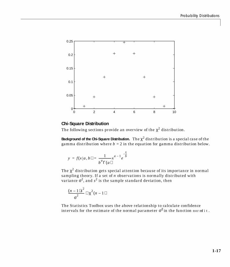
Example and Plot of the Binomial Distribution. The following commands generate aplot of the binomial pdf for n = 10 and p = 1/2.
x = 0:10;y = binopdf(x,10,0.5);plot(x,y,'+')
Probability Distributions
1-17
Chi-Square DistributionThe following sections provide an overview of the χ2 distribution.
Background of the Chi-Square Distribution. The χ2 distribution is a special case of thegamma distribution where b = 2 in the equation for gamma distribution below.
The χ2 distribution gets special attention because of its importance in normalsampling theory. If a set of n observations is normally distributed withvariance σ2, and s2 is the sample standard deviation, then
The Statistics Toolbox uses the above relationship to calculate confidenceintervals for the estimate of the normal parameter σ2 in the function normfit.
0 2 4 6 8 100
0.05
0.1
0.15
0.2
0.25
y f x a b,( ) 1
baΓ a( )------------------xa 1– e
xb---–
= =
n 1–( )s2
σ2----------------------- χ2 n 1–( )∼

1 Tutorial
1-18
Definition of the Chi-Square Distribution. The χ2 pdf is
where Γ( · ) is the Gamma function, and ν is the degrees of freedom.
Example and Plot of the Chi-Square Distribution. The χ2 distribution is skewed to theright especially for few degrees of freedom (ν). The plot shows the χ2
distribution with four degrees of freedom.
x = 0:0.2:15;y = chi2pdf(x,4);plot(x,y)
Noncentral Chi-Square DistributionThe following sections provide an overview of the noncentral χ2 distribution.
Background of the Noncentral Chi-Square Distribution. The χ2 distribution is actuallya simple special case of the noncentral chi-square distribution. One way togenerate random numbers with a χ2 distribution (with ν degrees of freedom) isto sum the squares of ν standard normal random numbers (mean equal to zero.)
What if we allow the normally distributed quantities to have a mean other thanzero? The sum of squares of these numbers yields the noncentral chi-squaredistribution. The noncentral chi-square distribution requires two parameters;the degrees of freedom and the noncentrality parameter. The noncentralityparameter is the sum of the squared means of the normally distributedquantities.
y f x ν( ) x ν 2–( ) 2⁄ e x– 2⁄
2
v2---
Γ ν 2⁄( )
-------------------------------------= =
0 5 10 150
0.05
0.1
0.15
0.2

Probability Distributions
1-19
The noncentral chi-square has scientific application in thermodynamics andsignal processing. The literature in these areas may refer to it as the Ricean orgeneralized Rayleigh distribution.
Definition of the Noncentral Chi-Square Distribution. There are many equivalentformulas for the noncentral chi-square distribution function. One formulationuses a modified Bessel function of the first kind. Another uses the generalizedLaguerre polynomials. The Statistics Toolbox computes the cumulativedistribution function values using a weighted sum of χ2 probabilities with theweights equal to the probabilities of a Poisson distribution. The Poissonparameter is one-half of the noncentrality parameter of the noncentralchi-square.
where δ is the noncentrality parameter.
Example of the Noncentral Chi-Square Distribution. The following commands generatea plot of the noncentral chi-square pdf.
x = (0:0.1:10)';p1 = ncx2pdf(x,4,2);p = chi2pdf(x,4);plot(x,p,'--',x,p1,'-')
F x ν δ,( )
12---δ� �� �
j
j!--------------e
δ2---–
� �� �� �� �� �
Pr χν 2 j+
2 x≤[ ]
j 0=
∞
�=
0 2 4 6 8 100
0.05
0.1
0.15
0.2

1 Tutorial
1-20
Discrete Uniform DistributionThe following sections provide an overview of the discrete uniform distribution.
Background of the Discrete Uniform Distribution. The discrete uniform distribution isa simple distribution that puts equal weight on the integers from one to N.
Definition of the Discrete Uniform Distribution. The discrete uniform pdf is
Example and Plot of the Discrete Uniform Distribution. As for all discrete distributions,the cdf is a step function. The plot shows the discrete uniform cdf for N = 10.
x = 0:10;y = unidcdf(x,10);stairs(x,y)set(gca,'Xlim',[0 11])
To pick a random sample of 10 from a list of 553 items:
numbers = unidrnd(553,1,10)
numbers =
293 372 5 213 37 231 380 326 515 468
y f x N( ) 1N---- I 1 … N, ,( ) x( )= =
0 2 4 6 8 100
0.2
0.4
0.6
0.8
1
Probability Distributions
1-21
Exponential DistributionThe following sections provide an overview of the exponential distribution.
Background of the Exponential Distribution. Like the chi-square distribution, theexponential distribution is a special case of the gamma distribution (obtainedby setting a = 1)
where Γ( · ) is the Gamma function.
The exponential distribution is special because of its utility in modeling eventsthat occur randomly over time. The main application area is in studies oflifetimes.
Definition of the Exponential Distribution. The exponential pdf is
Parameter Estimation for the Exponential Distribution. Suppose you are stress testinglight bulbs and collecting data on their lifetimes. You assume that theselifetimes follow an exponential distribution. You want to know how long youcan expect the average light bulb to last. Parameter estimation is the processof determining the parameters of the exponential distribution that fit this databest in some sense.
One popular criterion of goodness is to maximize the likelihood function. Thelikelihood has the same form as the exponential pdf above. But for the pdf, theparameters are known constants and the variable is x. The likelihood functionreverses the roles of the variables. Here, the sample values (the x’s) are alreadyobserved. So they are the fixed constants. The variables are the unknownparameters. MLE involves calculating the values of the parameters that givethe highest likelihood given the particular set of data.
y f x a b,( ) 1
baΓ a( )------------------xa 1– e
xb---–
= =
y f x µ( ) 1µ---e
xµ---–
= =
1 Tutorial
1-22
The function expfit returns the MLEs and confidence intervals for theparameters of the exponential distribution. Here is an example using randomnumbers from the exponential distribution with µ = 700.
lifetimes = exprnd(700,100,1);[muhat, muci] = expfit(lifetimes)
muhat =
672.8207
muci =
547.4338 810.9437
The MLE for parameter µ is 672, compared to the true value of 700. The 95%confidence interval for µ goes from 547 to 811, which includes the true value.
In our life tests we do not know the true value of µ so it is nice to have aconfidence interval on the parameter to give a range of likely values.
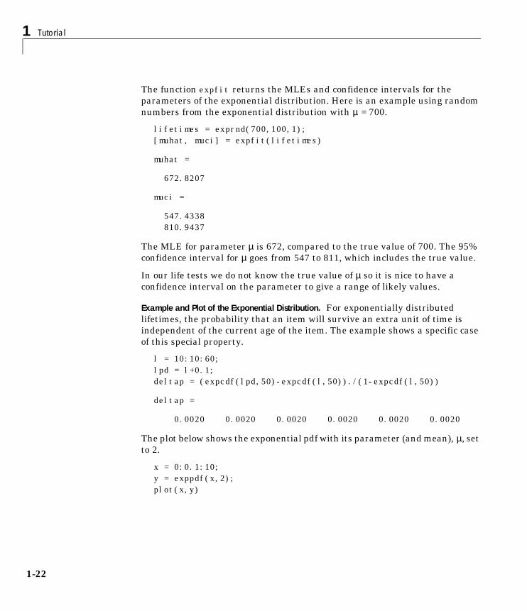
Example and Plot of the Exponential Distribution. For exponentially distributedlifetimes, the probability that an item will survive an extra unit of time isindependent of the current age of the item. The example shows a specific caseof this special property.
l = 10:10:60;lpd = l+0.1;deltap = (expcdf(lpd,50)-expcdf(l,50))./(1-expcdf(l,50))
deltap =
0.0020 0.0020 0.0020 0.0020 0.0020 0.0020
The plot below shows the exponential pdf with its parameter (and mean), µ, setto 2.
x = 0:0.1:10;y = exppdf(x,2);plot(x,y)

Probability Distributions
1-23
F DistributionThe following sections provide an overview of the F distribution.
Background of the F distribution. The F distribution has a natural relationship withthe chi-square distribution. If χ1 and χ2 are both chi-square with ν1 and ν2degrees of freedom respectively, then the statistic F below is F distributed.
The two parameters, ν1 and ν2, are the numerator and denominator degrees offreedom. That is, ν1 and ν2 are the number of independent pieces informationused to calculate χ1 and χ2 respectively.
Definition of the F distribution. The pdf for the F distribution is
where Γ( · ) is the Gamma function.
Example and Plot of the F distribution. The most common application of the Fdistribution is in standard tests of hypotheses in analysis of variance andregression.
0 2 4 6 8 100
0.1
0.2
0.3
0.4
0.5
F ν1 ν2,( )
χ1ν1------
χ2ν2------
------=
y f x ν1 ν2,( )Γ
ν1 ν2+( )2
-----------------------
Γν12------� �� � Γ
ν22------� �� �
--------------------------------ν1ν2------� �� �
ν1
2----- x
ν1 2–2
--------------
1ν1ν2------� �� � x+
ν1 ν2+2
-------------------------------------------------------------= =

1 Tutorial
1-24
The plot shows that the F distribution exists on the positive real numbers andis skewed to the right.
x = 0:0.01:10;y = fpdf(x,5,3);plot(x,y)
Noncentral F DistributionThe following sections provide an overview of the noncentral F distribution.
Background of the Noncentral F Distribution. As with the χ2 distribution, theF distribution is a special case of the noncentral F distribution. TheF distribution is the result of taking the ratio of two χ2 random variables eachdivided by its degrees of freedom.
If the numerator of the ratio is a noncentral chi-square random variabledivided by its degrees of freedom, the resulting distribution is the noncentralF distribution.
The main application of the noncentral F distribution is to calculate the powerof a hypothesis test relative to a particular alternative.
Definition of the Noncentral F Distribution. Similar to the noncentral χ2 distribution,the toolbox calculates noncentral F distribution probabilities as a weightedsum of incomplete beta functions using Poisson probabilities as the weights.
0 2 4 6 8 100
0.2
0.4
0.6
0.8
F x ν1 ν2 δ, ,( )
12---δ� �� �
j
j!--------------e
δ2---–
� �� �� �� �� �
Iν1 x⋅
ν2 ν+ 1 x⋅-------------------------ν12------ j+
ν22------,
� �� �� �
j 0=
∞
�=

Probability Distributions
1-25
I(x|a,b) is the incomplete beta function with parameters a and b, and δ is thenoncentrality parameter.
Example and Plot of the Noncentral F Distribution. The following commands generatea plot of the noncentral F pdf.
x = (0.01:0.1:10.01)';p1 = ncfpdf(x,5,20,10);p = fpdf(x,5,20);plot(x,p,'--',x,p1,'-')
Gamma DistributionThe following sections provide an overview of the gamma distribution.
Background of the Gamma Distribution. The gamma distribution is a family ofcurves based on two parameters. The chi-square and exponential distributions,which are children of the gamma distribution, are one-parameter distributionsthat fix one of the two gamma parameters.
The gamma distribution has the following relationship with the incompleteGamma function.
For b = 1 the functions are identical.
When a is large, the gamma distribution closely approximates a normaldistribution with the advantage that the gamma distribution has density onlyfor positive real numbers.
0 2 4 6 8 10 120
0.2
0.4
0.6
0.8
à x a b,( ) gammainc xb--- a,� �� �=

1 Tutorial
1-26
Definition of the Gamma Distribution. The gamma pdf is
where Γ( · ) is the Gamma function.
Parameter Estimation for the Gamma Distribution. Suppose you are stress testingcomputer memory chips and collecting data on their lifetimes. You assume thatthese lifetimes follow a gamma distribution. You want to know how long youcan expect the average computer memory chip to last. Parameter estimation isthe process of determining the parameters of the gamma distribution that fitthis data best in some sense.
One popular criterion of goodness is to maximize the likelihood function. Thelikelihood has the same form as the gamma pdf above. But for the pdf, theparameters are known constants and the variable is x. The likelihood functionreverses the roles of the variables. Here, the sample values (the x’s) are alreadyobserved. So they are the fixed constants. The variables are the unknownparameters. MLE involves calculating the values of the parameters that givethe highest likelihood given the particular set of data.
The function gamfit returns the MLEs and confidence intervals for theparameters of the gamma distribution. Here is an example using randomnumbers from the gamma distribution with a = 10 and b = 5.
lifetimes = gamrnd(10,5,100,1);[phat, pci] = gamfit(lifetimes)
phat =
10.9821 4.7258
pci =
7.4001 3.1543 14.5640 6.2974
Note phat(1) = and phat(2) = . The MLE for parameter a is 10.98,compared to the true value of 10. The 95% confidence interval for a goes from7.4 to 14.6, which includes the true value.
y f x a b,( ) 1
baΓ a( )------------------xa 1– e
xb---–
= =
a b

Probability Distributions
1-27
Similarly the MLE for parameter b is 4.7, compared to the true value of 5. The95% confidence interval for b goes from 3.2 to 6.3, which also includes the truevalue.
In our life tests we do not know the true value of a and b so it is nice to have aconfidence interval on the parameters to give a range of likely values.
Example and Plot of the Gamma Distribution. In the example the gamma pdf isplotted with the solid line. The normal pdf has a dashed line type.
x = gaminv((0.005:0.01:0.995),100,10);y = gampdf(x,100,10);y1 = normpdf(x,1000,100);plot(x,y,'-',x,y1,'-.')
Geometric DistributionThe following sections provide an overview of the geometric distribution.
Background of the Geometric Distribution. The geometric distribution is discrete,existing only on the nonnegative integers. It is useful for modeling the runs ofconsecutive successes (or failures) in repeated independent trials of a system.
The geometric distribution models the number of successes before one failurein an independent succession of tests where each test results in success orfailure.
700 800 900 1000 1100 1200 13000
1
2
3
4
5x 10⁻³

1 Tutorial
1-28
Definition of the Geometric Distribution. The geometric pdf is
where q = 1 – p.
Example and Plot of the Geometric Distribution. Suppose the probability of afive-year-old battery failing in cold weather is 0.03. What is the probability ofstarting 25 consecutive days during a long cold snap?
1 - geocdf(25,0.03)
ans =
0.4530
The plot shows the cdf for this scenario.
x = 0:25;y = geocdf(x,0.03);stairs(x,y)
Hypergeometric DistributionThe following sections provide an overview of the hypergeometric distribution.
Background of the Hypergeometric Distribution. The hypergeometric distributionmodels the total number of successes in a fixed size sample drawn withoutreplacement from a finite population.
The distribution is discrete, existing only for nonnegative integers less than thenumber of samples or the number of possible successes, whichever is greater.
y f x p( ) pqxI 0 1 …, ,( ) x( )= =
0 5 10 15 20 250
0.2
0.4
0.6
Probability Distributions
1-29
The hypergeometric distribution differs from the binomial only in that thepopulation is finite and the sampling from the population is withoutreplacement.
The hypergeometric distribution has three parameters that have directphysical interpretations. M is the size of the population. K is the number ofitems with the desired characteristic in the population. n is the number ofsamples drawn. Sampling “without replacement” means that once a particularsample is chosen, it is removed from the relevant population for all subsequentselections.
Definition of the Hypergeometric Distribution. The hypergeometric pdf is
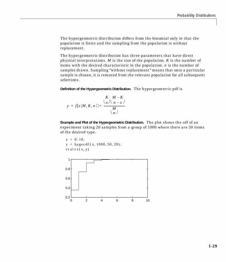
Example and Plot of the Hypergeometric Distribution. The plot shows the cdf of anexperiment taking 20 samples from a group of 1000 where there are 50 itemsof the desired type.
x = 0:10;y = hygecdf(x,1000,50,20);stairs(x,y)
y f x M K n, ,( )
Kx� �
� � M K–n x–� �
� �
Mn� �
� �-------------------------------= =
0 2 4 6 8 100.2
0.4
0.6
0.8
1
1 Tutorial
1-30
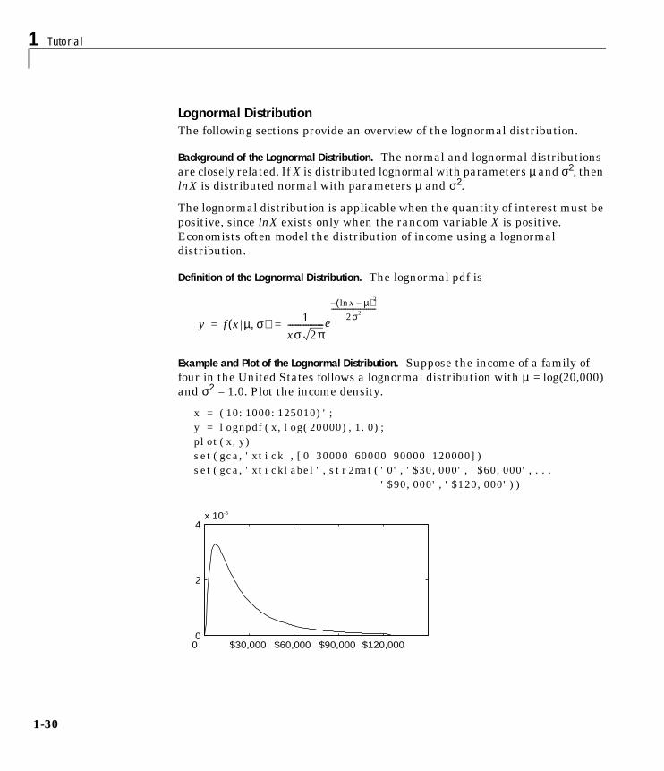
Lognormal DistributionThe following sections provide an overview of the lognormal distribution.
Background of the Lognormal Distribution. The normal and lognormal distributionsare closely related. If X is distributed lognormal with parameters µ and σ2, thenlnX is distributed normal with parameters µ and σ2.
The lognormal distribution is applicable when the quantity of interest must bepositive, since lnX exists only when the random variable X is positive.Economists often model the distribution of income using a lognormaldistribution.
Definition of the Lognormal Distribution. The lognormal pdf is
Example and Plot of the Lognormal Distribution. Suppose the income of a family offour in the United States follows a lognormal distribution with µ = log(20,000)and σ2 = 1.0. Plot the income density.
x = (10:1000:125010)';y = lognpdf(x,log(20000),1.0);plot(x,y)set(gca,'xtick',[0 30000 60000 90000 120000])set(gca,'xticklabel',str2mat('0','$30,000','$60,000',...
'$90,000','$120,000'))
y f x µ σ,( ) 1xσ 2π------------------e
lnx µ–( )– 2
2σ2----------------------------
= =
0 $30,000 $60,000 $90,000 $120,0000
2
4x 10⁻⁵
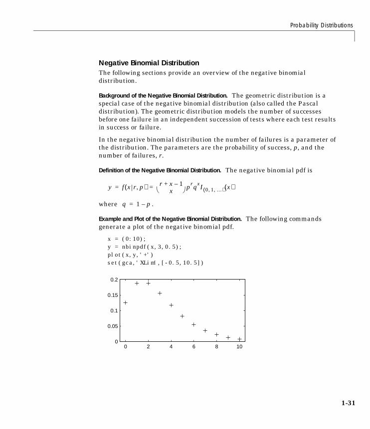
Probability Distributions
1-31
Negative Binomial DistributionThe following sections provide an overview of the negative binomialdistribution.
Background of the Negative Binomial Distribution. The geometric distribution is aspecial case of the negative binomial distribution (also called the Pascaldistribution). The geometric distribution models the number of successesbefore one failure in an independent succession of tests where each test resultsin success or failure.
In the negative binomial distribution the number of failures is a parameter ofthe distribution. The parameters are the probability of success, p, and thenumber of failures, r.
Definition of the Negative Binomial Distribution. The negative binomial pdf is
where .
Example and Plot of the Negative Binomial Distribution. The following commandsgenerate a plot of the negative binomial pdf.
x = (0:10);y = nbinpdf(x,3,0.5);plot(x,y,'+')set(gca,'XLim',[-0.5,10.5])
y f x r p,( ) r x 1–+x� �
� � prqxI 0 1 …, ,( ) x( )= =
q 1 p–=
0 2 4 6 8 100
0.05
0.1
0.15
0.2

1 Tutorial
1-32
Normal DistributionThe following sections provide an overview of the normal distribution.
Background of the Normal Distribution. The normal distribution is a two parameterfamily of curves. The first parameter, µ, is the mean. The second, σ, is thestandard deviation. The standard normal distribution (written Φ(x)) sets µ to 0and σ to 1.
Φ(x) is functionally related to the error function, erf.
The first use of the normal distribution was as a continuous approximation tothe binomial.
The usual justification for using the normal distribution for modeling is theCentral Limit Theorem, which states (roughly) that the sum of independentsamples from any distribution with finite mean and variance converges to thenormal distribution as the sample size goes to infinity.
Definition of the Normal Distribution. The normal pdf is
Parameter Estimation for the Normal Distribution. One of the first applications of thenormal distribution in data analysis was modeling the height of schoolchildren. Suppose we want to estimate the mean, µ, and the variance, σ2, of allthe 4th graders in the United States.
We have already introduced MLEs. Another desirable criterion in a statisticalestimator is unbiasedness. A statistic is unbiased if the expected value of thestatistic is equal to the parameter being estimated. MLEs are not alwaysunbiased. For any data sample, there may be more than one unbiasedestimator of the parameters of the parent distribution of the sample. Forinstance, every sample value is an unbiased estimate of the parameter µ of anormal distribution. The Minimum Variance Unbiased Estimator (MVUE) isthe statistic that has the minimum variance of all unbiased estimators of aparameter.
erf x( ) 2Φ x 2( ) 1–=
y f x µ σ,( ) 1σ 2π---------------e
x µ–( )– 2
2σ2----------------------
= =

Probability Distributions
1-33
The MVUEs of parameters µ and σ2 for the normal distribution are the sampleaverage and variance. The sample average is also the MLE for µ. There are twocommon textbook formulas for the variance.
They are
where
Equation 1 is the maximum likelihood estimator for σ2, and equation 2 is theMVUE.
The function normfit returns the MVUEs and confidence intervals for µ andσ2. Here is a playful example modeling the “heights” (inches) of a randomlychosen 4th grade class.
height = normrnd(50,2,30,1); % Simulate heights.[mu,s,muci,sci] = normfit(height)
mu = 50.2025
s = 1.7946
muci = 49.5210 50.8841
sci = 1.4292 2.4125
1) s2 1n---= xi x–( )2
i 1=
n
�
2) s2 1n 1–------------- xi x–( )2
i 1=
n
�=
xxin----
i 1=
n
�=

1 Tutorial
1-34
Example and Plot of the Normal Distribution. The plot shows the “bell” curve of thestandard normal pdf, with µ = 0 and σ = 1.
Poisson DistributionThe following sections provide an overview of the Poisson distribution.
Background of the Poisson Distribution. The Poisson distribution is appropriate forapplications that involve counting the number of times a random event occursin a given amount of time, distance, area, etc. Sample applications that involvePoisson distributions include the number of Geiger counter clicks per second,the number of people walking into a store in an hour, and the number of flawsper 1000 feet of video tape.
The Poisson distribution is a one parameter discrete distribution that takesnonnegative integer values. The parameter, λ, is both the mean and thevariance of the distribution. Thus, as the size of the numbers in a particularsample of Poisson random numbers gets larger, so does the variability of thenumbers.
As Poisson (1837) showed, the Poisson distribution is the limiting case of abinomial distribution where N approaches infinity and p goes to zero whileNp = λ.
The Poisson and exponential distributions are related. If the number of countsfollows the Poisson distribution, then the interval between individual countsfollows the exponential distribution.
-3 -2 -1 0 1 2 30
0.1
0.2
0.3
0.4

Probability Distributions
1-35
Definition of the Poisson Distribution. The Poisson pdf is
Parameter Estimation for the Poisson Distribution. The MLE and the MVUE of thePoisson parameter, λ, is the sample mean. The sum of independent Poissonrandom variables is also Poisson distributed with the parameter equal to thesum of the individual parameters. The Statistics Toolbox makes use of this factto calculate confidence intervals on λ. As λ gets large the Poisson distributioncan be approximated by a normal distribution with µ = λ and σ2 = λ. TheStatistics Toolbox uses this approximation for calculating confidence intervalsfor values of λ greater than 100.
Example and Plot of the Poisson Distribution. The plot shows the probability for eachnonnegative integer when λ = 5.
x = 0:15;y = poisspdf(x,5);plot(x,y,'+')
Rayleigh DistributionThe following sections provide an overview of the Rayleigh distribution.
Background of the Rayleigh Distribution. The Rayleigh distribution is a special caseof the Weibull distribution. If A and B are the parameters of the Weibulldistribution, then the Rayleigh distribution with parameter is equivalent tothe Weibull distribution with parameters and .
y f x λ( ) λx
x!-----e λ– I 0 1 …, ,( ) x( )= =
0 5 10 150
0.05
0.1
0.15
0.2
bA 1 2b2( )⁄= B 2=

1 Tutorial
1-36
If the component velocities of a particle in the x and y directions are twoindependent normal random variables with zero means and equal variances,then the distance the particle travels per unit time is distributed Rayleigh.
Definition of the Rayleigh Distribution. The Rayleigh pdf is
Parameter Estimation for the Rayleigh Distribution. The raylfit function returns theMLE of the Rayleigh parameter. This estimate is
Example and Plot of the Rayleigh Distribution. The following commands generate aplot of the Rayleigh pdf.
x = [0:0.01:2];p = raylpdf(x,0.5);plot(x,p)
y f x b( ) x
b2------e
x2–
2b2---------� �� �
= =
b 12n------- xi
2
i 1=
n
�=
0 0.5 1 1.5 20
0.5
1
1.5

Probability Distributions
1-37
Student’s t DistributionThe following sections provide an overview of Student’s t distribution.
Background of Student’s t Distribution. The t distribution is a family of curvesdepending on a single parameter ν (the degrees of freedom). As ν goes toinfinity, the t distribution converges to the standard normal distribution.
W. S. Gossett (1908) discovered the distribution through his work at theGuinness brewery. At that time, Guinness did not allow its staff to publish, soGossett used the pseudonym Student.
If x and s are the mean and standard deviation of an independent randomsample of size n from a normal distribution with mean µ and σ2 = n, then
Definition of Student’s t Distribution. Student’s t pdf is
where Γ( · ) is the Gamma function.
Example and Plot of Student’s t Distribution. The plot compares the t distributionwith ν = 5 (solid line) to the shorter tailed, standard normal distribution(dashed line).
x = -5:0.1:5;y = tpdf(x,5);z = normpdf(x,0,1);plot(x,y,'-',x,z,'-.')
t ν( ) x µ–s
------------=
ν n 1–=
y f x ν( )Γ ν 1+
2------------� �� �
Γ ν2---� �� �
----------------------1νπ
----------1
1 x2
ν-----+
� �� �
ν 1+2
--------------------------------------------= =

1 Tutorial
1-38
Noncentral t DistributionThe following sections provide an overview of the noncentral t distribution.
Background of the Noncentral t Distribution. The noncentral t distribution is ageneralization of the familiar Student’s t distribution.
If x and s are the mean and standard deviation of an independent randomsample of size n from a normal distribution with mean µ and σ2 = n, then
Suppose that the mean of the normal distribution is not µ. Then the ratio hasthe noncentral t distribution. The noncentrality parameter is the differencebetween the sample mean and µ.
The noncentral t distribution allows us to determine the probability that wewould detect a difference between x and µ in a t test. This probability is thepower of the test. As x-µ increases, the power of a test also increases.
Definition of the Noncentral t Distribution. The most general representation of thenoncentral t distribution is quite complicated. Johnson and Kotz (1970) give aformula for the probability that a noncentral t variate falls in the range [-t, t].
-5 0 50
0.1
0.2
0.3
0.4
t ν( ) x µ–s
------------=
ν n 1–=
Pr t–( ) x t< < ν δ,( )( )
12---δ2� �� �
j
j!-----------------e
δ2
2-----–
� �� �� �� �� �
Ix2
ν x2+
--------------- 12--- j+
ν2---,
� �� �� �
j 0=
∞
�=

Probability Distributions
1-39
I(x|a,b) is the incomplete beta function with parameters a and b, δ is thenoncentrality parameter, and ν is the degrees of freedom.
Example and Plot of the Noncentral t Distribution. The following commands generatea plot of the noncentral t pdf.
x = (-5:0.1:5)';p1 = nctcdf(x,10,1);p = tcdf(x,10);plot(x,p,'--',x,p1,'-')
Uniform (Continuous) DistributionThe following sections provide an overview of the uniform distribution.
Background of the Uniform Distribution. The uniform distribution (also calledrectangular) has a constant pdf between its two parameters a (the minimum)and b (the maximum). The standard uniform distribution (a = 0 and b = 1) is aspecial case of the beta distribution, obtained by setting both of its parametersto 1.
The uniform distribution is appropriate for representing the distribution ofround-off errors in values tabulated to a particular number of decimal places.
Definition of the Uniform Distribution. The uniform cdf is
Parameter Estimation for the Uniform Distribution. The sample minimum andmaximum are the MLEs of a and b respectively.
-5 0 50
0.2
0.4
0.6
0.8
1
p F x a b,( ) x a–b a–------------I a b,[ ] x( )= =

1 Tutorial
1-40
Example and Plot of the Uniform Distribution. The example illustrates the inversionmethod for generating normal random numbers using rand and norminv. Notethat the MATLAB function, randn, does not use inversion since it is notefficient for this case.
u = rand(1000,1);x = norminv(u,0,1);hist(x)
Weibull DistributionThe following sections provide an overview of the Weibull distribution.
Background of the Weibull Distribution. Waloddi Weibull (1939) offered thedistribution that bears his name as an appropriate analytical tool for modelingthe breaking strength of materials. Current usage also includes reliability andlifetime modeling. The Weibull distribution is more flexible than theexponential for these purposes.
To see why, consider the hazard rate function (instantaneous failure rate). Iff(t) and F(t) are the pdf and cdf of a distribution, then the hazard rate is
Substituting the pdf and cdf of the exponential distribution for f(t) and F(t)above yields a constant. The example below shows that the hazard rate for theWeibull distribution can vary.
-4 -2 0 2 40
100
200
300
h t( ) f t( )1 F t( )–--------------------=

Probability Distributions
1-41
Definition of the Weibull Distribution. The Weibull pdf is
Parameter Estimation for the Weibull Distribution. Suppose we want to model thetensile strength of a thin filament using the Weibull distribution. The functionweibfit gives MLEs and confidence intervals for the Weibull parameters.
strength = weibrnd(0.5,2,100,1); % Simulated strengths.[p,ci] = weibfit(strength)
p = 0.4746 1.9582
ci = 0.3851 1.6598 0.5641 2.2565
The default 95% confidence interval for each parameter contains the truevalue.
Example and Plot of the Weibull Distribution. The exponential distribution has aconstant hazard function, which is not generally the case for the Weibulldistribution.
The plot shows the hazard functions for exponential (dashed line) and Weibull(solid line) distributions having the same mean life. The Weibull hazard ratehere increases with age (a reasonable assumption).
t = 0:0.1:3;h1 = exppdf(t,0.6267) ./ (1-expcdf(t,0.6267));h2 = weibpdf(t,2,2) ./ (1-weibcdf(t,2,2));plot(t,h1,'--',t,h2,'-')
y f x a b,( ) abxb 1– e axb– I 0 ∞,( ) x( )= =

1 Tutorial
1-42
0 0.5 1 1.5 2 2.5 30
5
10
15

Descriptive Statistics
1-43
Descriptive StatisticsData samples can have thousands (even millions) of values. Descriptivestatistics are a way to summarize this data into a few numbers that containmost of the relevant information. The following sections explore the featuresprovided by the Statistics Toolbox for working with descriptive statistics:
• “Measures of Central Tendency (Location)”
• “Measures of Dispersion”
• “Functions for Data with Missing Values (NaNs)”
• “Function for Grouped Data”
• “Percentiles and Graphical Descriptions”
• “The Bootstrap”
Measures of Central Tendency (Location)The purpose of measures of central tendency is to locate the data values on thenumber line. Another term for these statistics is measures of location.
The table gives the function names and descriptions.
The average is a simple and popular estimate of location. If the data samplecomes from a normal distribution, then the sample average is also optimal(MVUE of µ).
Measures of Location
geomean Geometric mean
harmmean Harmonic mean
mean Arithmetic average (in MATLAB)
median 50th percentile (in MATLAB)
trimmean Trimmed mean

1 Tutorial
1-44
Unfortunately, outliers, data entry errors, or glitches exist in almost all realdata. The sample average is sensitive to these problems. One bad data valuecan move the average away from the center of the rest of the data by anarbitrarily large distance.
The median and trimmed mean are two measures that are resistant (robust) tooutliers. The median is the 50th percentile of the sample, which will onlychange slightly if you add a large perturbation to any value. The idea behindthe trimmed mean is to ignore a small percentage of the highest and lowestvalues of a sample when determining the center of the sample.
The geometric mean and harmonic mean, like the average, are not robust tooutliers. They are useful when the sample is distributed lognormal or heavilyskewed.
The example below shows the behavior of the measures of location for a samplewith one outlier.
x = [ones(1,6) 100]
x = 1 1 1 1 1 1 100
locate = [geomean(x) harmmean(x) mean(x) median(x)... trimmean(x,25)]
locate =
1.9307 1.1647 15.1429 1.0000 1.0000
You can see that the mean is far from any data value because of the influenceof the outlier. The median and trimmed mean ignore the outlying value anddescribe the location of the rest of the data values.

Descriptive Statistics
1-45
Measures of DispersionThe purpose of measures of dispersion is to find out how spread out the datavalues are on the number line. Another term for these statistics is measures ofspread.
The table gives the function names and descriptions.
The range (the difference between the maximum and minimum values) is thesimplest measure of spread. But if there is an outlier in the data, it will be theminimum or maximum value. Thus, the range is not robust to outliers.
The standard deviation and the variance are popular measures of spread thatare optimal for normally distributed samples. The sample variance is theMVUE of the normal parameter σ2. The standard deviation is the square rootof the variance and has the desirable property of being in the same units as thedata. That is, if the data is in meters, the standard deviation is in meters aswell. The variance is in meters2, which is more difficult to interpret.
Neither the standard deviation nor the variance is robust to outliers. A datavalue that is separate from the body of the data can increase the value of thestatistics by an arbitrarily large amount.
The Mean Absolute Deviation (MAD) is also sensitive to outliers. But the MADdoes not move quite as much as the standard deviation or variance in responseto bad data.
The Interquartile Range (IQR) is the difference between the 75th and 25thpercentile of the data. Since only the middle 50% of the data affects thismeasure, it is robust to outliers.
Measures of Dispersion
iqr Interquartile Range
mad Mean Absolute Deviation
range Range
std Standard deviation (in MATLAB)
var Variance (in MATLAB)

1 Tutorial
1-46
The example below shows the behavior of the measures of dispersion for asample with one outlier.
x = [ones(1,6) 100]
x = 1 1 1 1 1 1 100
stats = [iqr(x) mad(x) range(x) std(x)]
stats = 0 24.2449 99.0000 37.4185
Functions for Data with Missing Values (NaNs)Most real-world data sets have one or more missing elements. It is convenientto code missing entries in a matrix as NaN (Not a Number).
Here is a simple example.
m = magic(3);m([1 5]) = [NaN NaN]
m =NaN 1 63 NaN 74 9 2
Any arithmetic operation that involves the missing values in this matrix yieldsNaN, as below.
sum(m)
ans =
NaN NaN 15
Removing cells with NaN would destroy the matrix structure. Removing wholerows that contain NaN would discard real data. Instead, the Statistics Toolboxhas a variety of functions that are similar to other MATLAB functions, but thattreat NaN values as missing and therefore ignore them in the calculations.

Descriptive Statistics
1-47
nansum(m)
ans =
7 10 13
In addition, other Statistics Toolbox functions operate only on the numericvalues, ignoring NaNs. These include iqr, kurtosis, mad, prctile, range,skewness, and trimmean.
Function for Grouped DataAs we saw in the previous section, the descriptive statistics functions cancompute statistics on each column in a matrix. Sometimes, however, you mayhave your data arranged differently so that measurements appear in onecolumn or variable, and a grouping code appears in a second column orvariable. Although MATLAB’s syntax makes it simple to apply functions to asubset of an array, in this case it is simpler to use the grpstats function.
The grpstats function can compute the mean, standard error of the mean, andcount (number of observations) for each group defined by one or more groupingvariables. If you supply a significance level, it also creates a graph of the groupmeans with confidence intervals.
As an example, load the larger car data set. We can look at the average valueof MPG (miles per gallon) for cars grouped by org (location of the origin of thecar).
NaN Functions
nanmax Maximum ignoring NaNs
nanmean Mean ignoring NaNs
nanmedian Median ignoring NaNs
nanmin Minimum ignoring NaNs
nanstd Standard deviation ignoring NaNs
nansum Sum ignoring NaNs

1 Tutorial
1-48
load carbiggrpstats(MPG,org,0.05)ans = 20.084 27.891 30.451
We can also get the complete set of statistics for MPG grouped by three variables:org, cyl4 (the engine has four cylinders or not), and when (when the car wasmade).
[m,s,c,n] = grpstats(MPG,{org cyl4 when});[n num2cell([m s c])]
ans =
'USA' 'Other' 'Early' [14.896] [0.33306] [77] 'USA' 'Other' 'Mid' [17.479] [0.30225] [75] 'USA' 'Other' 'Late' [21.536] [0.97961] [25] 'USA' 'Four' 'Early' [23.333] [0.87328] [12] 'USA' 'Four' 'Mid' [27.027] [0.75456] [22] 'USA' 'Four' 'Late' [29.734] [0.71126] [38] 'Europe' 'Other' 'Mid' [ 17.5] [ 0.9478] [ 4] 'Europe' 'Other' 'Late' [30.833] [ 3.1761] [ 3]
USA Europe Japan18
20
22
24
26
28
30
32
Group
Mea
n
Means and Confidence Intervals for Each Group
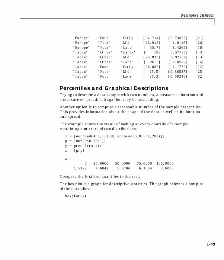
Descriptive Statistics
1-49
'Europe' 'Four' 'Early' [24.714] [0.73076] [21] 'Europe' 'Four' 'Mid' [26.912] [ 1.0116] [26] 'Europe' 'Four' 'Late' [ 35.7] [ 1.4265] [16] 'Japan' 'Other' 'Early' [ 19] [0.57735] [ 3] 'Japan' 'Other' 'Mid' [20.833] [0.92796] [ 3] 'Japan' 'Other' 'Late' [ 26.5] [ 2.0972] [ 4] 'Japan' 'Four' 'Early' [26.083] [ 1.1772] [12] 'Japan' 'Four' 'Mid' [ 29.5] [0.86547] [25] 'Japan' 'Four' 'Late' [ 35.3] [0.68346] [32]
Percentiles and Graphical DescriptionsTrying to describe a data sample with two numbers, a measure of location anda measure of spread, is frugal but may be misleading.
Another option is to compute a reasonable number of the sample percentiles.This provides information about the shape of the data as well as its locationand spread.
The example shows the result of looking at every quartile of a samplecontaining a mixture of two distributions.
x = [normrnd(4,1,1,100) normrnd(6,0.5,1,200)];p = 100*(0:0.25:1);y = prctile(x,p);z = [p;y]
z = 0 25.0000 50.0000 75.0000 100.0000 1.5172 4.6842 5.6706 6.1804 7.6035
Compare the first two quantiles to the rest.
The box plot is a graph for descriptive statistics. The graph below is a box plotof the data above.
boxplot(x)

1 Tutorial
1-50
The long lower tail and plus signs show the lack of symmetry in the samplevalues. For more information on box plots, see “Statistical Plots” on page 1-128.
The histogram is a complementary graph.
hist(x)
The BootstrapIn recent years the statistical literature has examined the properties ofresampling as a means to acquire information about the uncertainty ofstatistical estimators.
The bootstrap is a procedure that involves choosing random samples withreplacement from a data set and analyzing each sample the same way.Sampling with replacement means that every sample is returned to the data setafter sampling. So a particular data point from the original data set couldappear multiple times in a given bootstrap sample. The number of elements ineach bootstrap sample equals the number of elements in the original data set.
1
2
3
4
5
6
7
Val
ues
Column Number
1 2 3 4 5 6 7 80
20
40
60
80
100

Descriptive Statistics
1-51
The range of sample estimates we obtain allows us to establish the uncertaintyof the quantity we are estimating.
Here is an example taken from Efron and Tibshirani (1993) comparing LawSchool Admission Test (LSAT) scores and subsequent law school grade pointaverage (GPA) for a sample of 15 law schools.
load lawdataplot(lsat,gpa,'+')lsline
The least squares fit line indicates that higher LSAT scores go with higher lawschool GPAs. But how sure are we of this conclusion? The plot gives us someintuition but nothing quantitative.
We can calculate the correlation coefficient of the variables using the corrcoeffunction.
rhohat = corrcoef(lsat,gpa)
rhohat =
1.0000 0.7764 0.7764 1.0000
Now we have a number, 0.7764, describing the positive connection betweenLSAT and GPA, but though 0.7764 may seem large, we still do not know if it isstatistically significant.
Using the bootstrp function we can resample the lsat and gpa vectors asmany times as we like and consider the variation in the resulting correlationcoefficients.
540 560 580 600 620 640 660 6802.6
2.8
3
3.2
3.4
3.6

1 Tutorial
1-52
Here is an example.
rhos1000 = bootstrp(1000,'corrcoef',lsat,gpa);
This command resamples the lsat and gpa vectors 1000 times and computesthe corrcoef function on each sample. Here is a histogram of the result.
hist(rhos1000(:,2),30)
Nearly all the estimates lie on the interval [0.4 1.0].
This is strong quantitative evidence that LSAT and subsequent GPA arepositively correlated. Moreover, it does not require us to make any strongassumptions about the probability distribution of the correlation coefficient.
0.2 0.4 0.6 0.8 10
20
40
60
80
100
Cluster Analysis
1-53
Cluster AnalysisCluster analysis, also called segmentation analysis or taxonomy analysis, is away to partition a set of objects into groups, or clusters, in such a way that theprofiles of objects in the same cluster are very similar and the profiles of objectsin different clusters are quite distinct.
Cluster analysis can be performed on many different types of data sets. Forexample, a data set might contain a number of observations of subjects in astudy where each observation contains a set of variables.
Many different fields of study, such as engineering, zoology, medicine,linguistics, anthropology, psychology, and marketing, have contributed to thedevelopment of clustering techniques and the application of such techniques.For example, cluster analysis can be used to find two similar groups for theexperiment and control groups in a study. In this way, if statistical differencesare found in the groups, they can be attributed to the experiment and not toany initial difference between the groups.
The following sections explore the clustering features in the Statistics Toolbox:
• “Terminology and Basic Procedure”
• “Finding the Similarities Between Objects”
• “Defining the Links Between Objects”
• “Evaluating Cluster Formation”
• “Creating Clusters”
Terminology and Basic ProcedureTo perform cluster analysis on a data set using the Statistics Toolbox functions,follow this procedure:
1 Find the similarity or dissimilarity between every pair of objects in thedata set. In this step, you calculate the distance between objects using thepdist function. The pdist function supports many different ways tocompute this measurement. See “Finding the Similarities Between Objects”on page 1-54 for more information.
2 Group the objects into a binary, hierarchical cluster tree. In this step,you link together pairs of objects that are in close proximity using the

1 Tutorial
1-54
linkage function. The linkage function uses the distance informationgenerated in step 1 to determine the proximity of objects to each other. Asobjects are paired into binary clusters, the newly formed clusters aregrouped into larger clusters until a hierarchical tree is formed. See “Definingthe Links Between Objects” on page 1-56 for more information.
3 Determine where to divide the hierarchical tree into clusters. In thisstep, you divide the objects in the hierarchical tree into clusters using thecluster function. The cluster function can create clusters by detectingnatural groupings in the hierarchical tree or by cutting off the hierarchicaltree at an arbitrary point. See “Creating Clusters” on page 1-64 for moreinformation.
The following sections provide more information about each of these steps.
Note The Statistics Toolbox includes a convenience function, clusterdata,which performs all these steps for you. You do not need to execute the pdist,linkage, or cluster functions separately. However, the clusterdata functiondoes not give you access to the options each of the individual routines offers.For example, if you use the pdist function you can choose the distancecalculation method, whereas if you use the clusterdata function you cannot.
Finding the Similarities Between ObjectsYou use the pdist function to calculate the distance between every pair ofobjects in a data set. For a data set made up of m objects, there are
pairs in the data set. The result of this computation is commonlyknown as a similarity matrix (or dissimilarity matrix).
There are many ways to calculate this distance information. By default, thepdist function calculates the Euclidean distance between objects; however,you can specify one of several other options. See pdist for more information.
m m 1–( )⋅ 2⁄

Cluster Analysis
1-55
Note You can optionally normalize the values in the data set beforecalculating the distance information. In a real world data set, variables can bemeasured against different scales. For example, one variable can measureIntelligence Quotient (IQ) test scores and another variable can measure headcircumference. These discrepancies can distort the proximity calculations.Using the zscore function, you can convert all the values in the data set to usethe same proportional scale. See zscore for more information.
For example, consider a data set, X, made up of five objects where each objectis a set of x,y coordinates.
• Object 1: 1, 2
• Object 2: 2.5, 4.5
• Object 3: 2, 2
• Object 4: 4, 1.5
• Object 5: 4, 2.5
You can define this data set as a matrix
X = [1 2;2.5 4.5;2 2;4 1.5;4 2.5]
and pass it to pdist. The pdist function calculates the distance betweenobject 1 and object 2, object 1 and object 3, and so on until the distancesbetween all the pairs have been calculated. The following figure plots theseobjects in a graph. The distance between object 2 and object 3 is shown toillustrate one interpretation of distance.
1
1
5
2 43
4
3
2
5
distance
1 3 4
5
2

1 Tutorial
1-56
Returning Distance Information The pdist function returns this distance information in a vector, Y, where eachelement contains the distance between a pair of objects.
Y = pdist(X)
Y =
Columns 1 through 7 2.9155 1.0000 3.0414 3.0414 2.5495 3.3541 2.5000 Columns 8 through 10 2.0616 2.0616 1.0000
To make it easier to see the relationship between the distance informationgenerated by pdist and the objects in the original data set, you can reformatthe distance vector into a matrix using the squareform function. In this matrix,element i,j corresponds to the distance between object i and object j in theoriginal data set. In the following example, element 1,1 represents the distancebetween object 1 and itself (which is zero). Element 1,2 represents the distancebetween object 1 and object 2, and so on.
squareform(Y)
ans = 0 2.9155 1.0000 3.0414 3.0414 2.9155 0 2.5495 3.3541 2.5000 1.0000 2.5495 0 2.0616 2.0616 3.0414 3.3541 2.0616 0 1.0000 3.0414 2.5000 2.0616 1.0000 0
Defining the Links Between ObjectsOnce the proximity between objects in the data set has been computed, you candetermine which objects in the data set should be grouped together intoclusters, using the linkage function. The linkage function takes the distanceinformation generated by pdist and links pairs of objects that are closetogether into binary clusters (clusters made up of two objects). The linkagefunction then links these newly formed clusters to other objects to create biggerclusters until all the objects in the original data set are linked together in ahierarchical tree.
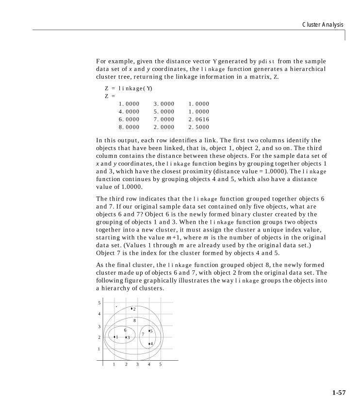
Cluster Analysis
1-57
For example, given the distance vector Y generated by pdist from the sampledata set of x and y coordinates, the linkage function generates a hierarchicalcluster tree, returning the linkage information in a matrix, Z.
Z = linkage(Y)Z = 1.0000 3.0000 1.0000 4.0000 5.0000 1.0000 6.0000 7.0000 2.0616 8.0000 2.0000 2.5000
In this output, each row identifies a link. The first two columns identify theobjects that have been linked, that is, object 1, object 2, and so on. The thirdcolumn contains the distance between these objects. For the sample data set ofx and y coordinates, the linkage function begins by grouping together objects 1and 3, which have the closest proximity (distance value = 1.0000). The linkagefunction continues by grouping objects 4 and 5, which also have a distancevalue of 1.0000.
The third row indicates that the linkage function grouped together objects 6and 7. If our original sample data set contained only five objects, what areobjects 6 and 7? Object 6 is the newly formed binary cluster created by thegrouping of objects 1 and 3. When the linkage function groups two objectstogether into a new cluster, it must assign the cluster a unique index value,starting with the value m+1, where m is the number of objects in the originaldata set. (Values 1 through m are already used by the original data set.)Object 7 is the index for the cluster formed by objects 4 and 5.
As the final cluster, the linkage function grouped object 8, the newly formedcluster made up of objects 6 and 7, with object 2 from the original data set. Thefollowing figure graphically illustrates the way linkage groups the objects intoa hierarchy of clusters.
1
1
5
2 43
4
3
2
5
67
8
1
2
34
5
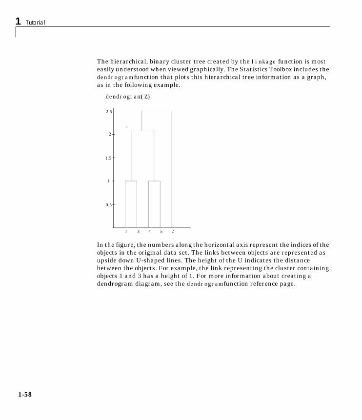
1 Tutorial
1-58
The hierarchical, binary cluster tree created by the linkage function is mosteasily understood when viewed graphically. The Statistics Toolbox includes thedendrogram function that plots this hierarchical tree information as a graph,as in the following example.
dendrogram(Z)
In the figure, the numbers along the horizontal axis represent the indices of theobjects in the original data set. The links between objects are represented asupside down U-shaped lines. The height of the U indicates the distancebetween the objects. For example, the link representing the cluster containingobjects 1 and 3 has a height of 1. For more information about creating adendrogram diagram, see the dendrogram function reference page.
0.5
1
2.5
3 54
2
1.5
1
2

Cluster Analysis
1-59
Evaluating Cluster FormationAfter linking the objects in a data set into a hierarchical cluster tree, you maywant to verify that the tree represents significant similarity groupings. Inaddition, you may want more information about the links between the objects.The Statistics Toolbox provides functions to perform both these tasks, asdescribed in the following sections:
• “Verifying the Cluster Tree”
• “Getting More Information About Cluster Links”
Verifying the Cluster TreeOne way to measure the validity of the cluster information generated by thelinkage function is to compare it with the original proximity data generated bythe pdist function. If the clustering is valid, the linking of objects in the clustertree should have a strong correlation with the distances between objects in thedistance vector. The cophenet function compares these two sets of values andcomputes their correlation, returning a value called the cophenetic correlationcoefficient. The closer the value of the cophenetic correlation coefficient is to 1,the better the clustering solution.
You can use the cophenetic correlation coefficient to compare the results ofclustering the same data set using different distance calculation methods orclustering algorithms.
For example, you can use the cophenet function to evaluate the clusterscreated for the sample data set
c = cophenet(Z,Y)c = 0.8573
where Z is the matrix output by the linkage function and Y is the distancevector output by the pdist function.
Execute pdist again on the same data set, this time specifying the City Blockmetric. After running the linkage function on this new pdist output, use thecophenet function to evaluate the clustering using a different distance metric.
c = cophenet(Z,Y)c =
0.9289

1 Tutorial
1-60
The cophenetic correlation coefficient shows a stronger correlation when theCity Block metric is used.
Getting More Information About Cluster LinksOne way to determine the natural cluster divisions in a data set is to comparethe length of each link in a cluster tree with the lengths of neighboring linksbelow it in the tree.
If a link is approximately the same length as neighboring links, it indicatesthat there are similarities between the objects joined at this level of thehierarchy. These links are said to exhibit a high level of consistency.
If the length of a link differs from neighboring links, it indicates that there aredissimilarities between the objects at this level in the cluster tree. This link issaid to be inconsistent with the links around it. In cluster analysis,inconsistent links can indicate the border of a natural division in a data set.The cluster function uses a measure of inconsistency to determine where todivide a data set into clusters. (See “Creating Clusters” on page 1-64 for moreinformation.)
The next section provides an example.
Example: Inconsistent Links. To illustrate, the following example creates a data setof random numbers with three deliberate natural groupings. In thedendrogram, note how the objects tend to collect into three groups. These threegroups are then connected by three longer links. These longer links areinconsistent when compared with the links below them in the hierarchy.
rand('seed',3)X = [rand(10,2)+1;rand(10,2)+2;rand(10,2)+3];Y = pdist(X);Z = linkage(Y);dendrogram(Z);

Cluster Analysis
1-61
The relative consistency of each link in a hierarchical cluster tree can bequantified and expressed as the inconsistency coefficient. This value comparesthe length of a link in a cluster hierarchy with the average length ofneighboring links. If the object is consistent with those around it, it will have alow inconsistency coefficient. If the object is inconsistent with those around it,it will have a higher inconsistency coefficient.
To generate a listing of the inconsistency coefficient for each link the clustertree, use the inconsistent function. The inconsistent function compareseach link in the cluster hierarchy with adjacent links two levels below it in thecluster hierarchy. This is called the depth of the comparison. Using theinconsistent function, you can specify other depths. The objects at the bottomof the cluster tree, called leaf nodes, that have no further objects below them,have an inconsistency coefficient of zero.
0
0.1
0.2
0.3
0.4
0.5
0.6
0.7
23 25 29 30 27 28 26 24 21 22 11 12 15 13 16 18 20 14 17 19 1 2 7 3 6 8 9 10 4 5
These links show consistency.
These links show inconsistency when compared to links below them.

1 Tutorial
1-62
For example, returning to the sample data set of x and y coordinates, we canuse the inconsistent function to calculate the inconsistency values for thelinks created by the linkage function, described in “Defining the LinksBetween Objects” on page 1-56.
I = inconsistent(Z)I = 1.0000 0 1.0000 0 1.0000 0 1.0000 0 1.3539 0.8668 3.0000 0.8165 2.2808 0.3100 2.0000 0.7071
The inconsistent function returns data about the links in an (m-1)-by-4matrix where each column provides data about the links.
In the sample output, the first row represents the link between objects 1 and 3.(This cluster is assigned the index 6 by the linkage function.) Because this aleaf node, the inconsistency coefficient is zero. The second row represents thelink between objects 4 and 5, also a leaf node. (This cluster is assigned theindex 7 by the linkage function.)
The third row evaluates the link that connects these two leaf nodes, objects 6and 7. (This cluster is called object 8 in the linkage output). Column threeindicates that three links are considered in the calculation: the link itself andthe two links directly below it in the hierarchy. Column one represents themean of the lengths of these links. The inconsistent function uses the lengthinformation output by the linkage function to calculate the mean. Column tworepresents the standard deviation between the links. The last column containsthe inconsistency value for these links, 0.8165.
Column Description
1 Mean of the lengths of all the links included in the calculation
2 Standard deviation of all the links included in the calculation
3 Number of links included in the calculation
4 Inconsistency coefficient
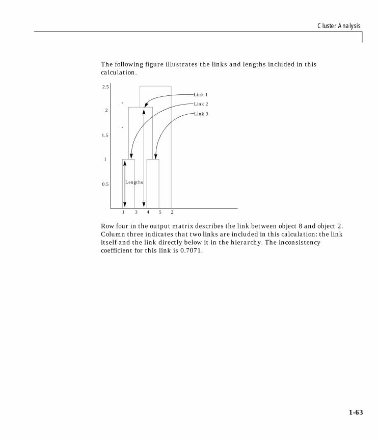
Cluster Analysis
1-63
The following figure illustrates the links and lengths included in thiscalculation.
Row four in the output matrix describes the link between object 8 and object 2.Column three indicates that two links are included in this calculation: the linkitself and the link directly below it in the hierarchy. The inconsistencycoefficient for this link is 0.7071.
0.5
1
2.5
3 54
2
1.5
1
2
Link 1
Lengths
Link 2
Link 3

1 Tutorial
1-64
The following figure illustrates the links and lengths included in thiscalculation.
Creating Clusters After you create the hierarchical tree of binary clusters, you can divide thehierarchy into larger clusters using the cluster function. The clusterfunction lets you create clusters in two ways, as discussed in the followingsections:
• “Finding the Natural Divisions in the Data Set”
• “Specifying Arbitrary Clusters”
Finding the Natural Divisions in the Data SetIn the hierarchical cluster tree, the data set may naturally align itself intoclusters. This can be particularly evident in a dendrogram diagram wheregroups of objects are densely packed in certain areas and not in others. Theinconsistency coefficient of the links in the cluster tree can identify these pointswhere the similarities between objects change. (See “Evaluating ClusterFormation” on page 1-59 for more information about the inconsistencycoefficient.) You can use this value to determine where the cluster functiondraws cluster boundaries.
0.5
1
2.5
3 54
2
1.5
1
2
Link 1
Lengths
Link 2
Cluster Analysis
1-65
For example, if you use the cluster function to group the sample data set intoclusters, specifying an inconsistency coefficient threshold of 0.9 as the value ofthe cutoff argument, the cluster function groups all the objects in the sampledata set into one cluster. In this case, none of the links in the cluster hierarchyhad an inconsistency coefficient greater than 0.9.
T = cluster(Z,0.9)T = 1 1 1 1 1
The cluster function outputs a vector, T, that is the same size as the originaldata set. Each element in this vector contains the number of the cluster intowhich the corresponding object from the original data set was placed.
If you lower the inconsistency coefficient threshold to 0.8, the cluster functiondivides the sample data set into three separate clusters.
T = cluster(Z,0.8)T =
13122
This output indicates that objects 1 and 3 were placed in cluster 1, objects 4and 5 were placed in cluster 2, and object 2 was placed in cluster 3.
Specifying Arbitrary ClustersInstead of letting the cluster function create clusters determined by thenatural divisions in the data set, you can specify the number of clusters youwant created. In this case, the value of the cutoff argument specifies the pointin the cluster hierarchy at which to create the clusters.
For example, you can specify that you want the cluster function to divide thesample data set into two clusters. In this case, the cluster function creates onecluster containing objects 1, 3, 4, and 5 and another cluster containing object 2.

1 Tutorial
1-66
T = cluster(Z,2)T =
12111
To help you visualize how the cluster function determines how to create theseclusters, the following figure shows the dendrogram of the hierarchical clustertree. When you specify a value of 2, the cluster function draws an imaginaryhorizontal line across the dendrogram that bisects two vertical lines. All theobjects below the line belong to one of these two clusters.
If you specify a cutoff value of 3, the cluster function cuts off the hierarchyat a lower point, bisecting three lines.
T = cluster(Z,3)T =
13122
0.5
1
2.5
3 54
2
1.5
1
2
cutoff = 2
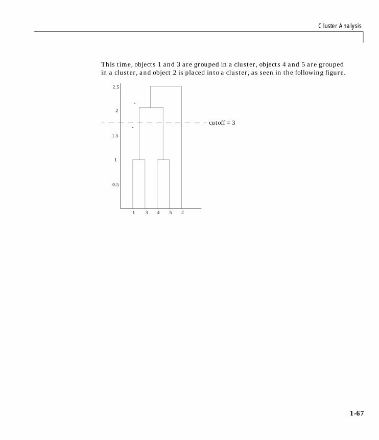
Cluster Analysis
1-67
This time, objects 1 and 3 are grouped in a cluster, objects 4 and 5 are groupedin a cluster, and object 2 is placed into a cluster, as seen in the following figure.
0.5
1
2.5
3 54
2
1.5
1
2
cutoff = 3
1 Tutorial
1-68
Linear ModelsLinear models represent the relationship between a continuous responsevariable and one or more predictor variables (either continuous or categorical)in the form
where:
• y is an n-by-1 vector of observations of the response variable.
• X is the n-by-p design matrix determined by the predictors.
• β is a p-by-1 vector of parameters.
• ε is an n-by-1 vector of random disturbances, independent of each other andusually having a normal distribution.
MATLAB uses this general form of the linear model to solve a variety of specificregression and analysis of variance (ANOVA) problems. For example, forpolynomial and multiple regression problems, the columns of X are predictorvariable values or powers of such values. For one-way, two-way, andhigher-way ANOVA models, the columns of X are dummy (or indicator)variables that encode the predictor categories. For analysis of covariance(ANOCOVA) models, X contains values of a continuous predictor and codes fora categorical predictor.
The following sections describe a number of functions for fitting various typesof linear models:
• “One-Way Analysis of Variance (ANOVA)”
• “Two-Way Analysis of Variance (ANOVA)”
• “N-Way Analysis of Variance”
• “Multiple Linear Regression”
• “Quadratic Response Surface Models”
• “Stepwise Regression”
• “Generalized Linear Models”
• “Robust and Nonparametric Methods”
y Xβ ε+=

Linear Models
1-69
See the sections below for a tour of some of the related graphical tools:
• “The polytool Demo” on page 1-156
• “The aoctool Demo” on page 1-161
• “The rsmdemo Demo” on page 1-170
One-Way Analysis of Variance (ANOVA)The purpose of one-way ANOVA is to find out whether data from severalgroups have a common mean. That is, to determine whether the groups areactually different in the measured characteristic.
One-way ANOVA is a simple special case of the linear model. The one-wayANOVA form of the model is
where:
• yij is a matrix of observations in which each column represents a differentgroup.
• α.j is a matrix whose columns are the group means. (The “dot j” notationmeans that α applies to all rows of the jth column. That is, the value αij isthe same for all i.)
• εij is a matrix of random disturbances.
The model posits that the columns of y are a constant plus a randomdisturbance. You want to know if the constants are all the same.
The following sections explore one-way ANOVA in greater detail:
• “Example: One-Way ANOVA”
• “Multiple Comparisons”
Example: One-Way ANOVAThe data below comes from a study by Hogg and Ledolter (1987) of bacteriacounts in shipments of milk. The columns of the matrix hogg representdifferent shipments. The rows are bacteria counts from cartons of milk chosenrandomly from each shipment. Do some shipments have higher counts thanothers?
yij α.j εij+=

1 Tutorial
1-70
load hogghogg
hogg =
24 14 11 7 19 15 7 9 7 24 21 12 7 4 19 27 17 13 7 15 33 14 12 12 10 23 16 18 18 20
[p,tbl,stats] = anova1(hogg);p
p = 1.1971e-04
The standard ANOVA table has columns for the sums of squares, degrees offreedom, mean squares (SS/df), F statistic, and p-value.
You can use the F statistic to do a hypothesis test to find out if the bacteriacounts are the same. anova1 returns the p-value from this hypothesis test.
In this case the p-value is about 0.0001, a very small value. This is a strongindication that the bacteria counts from the different tankers are not the same.An F statistic as extreme as the observed F would occur by chance only once in10,000 times if the counts were truly equal.
The p-value returned by anova1 depends on assumptions about the randomdisturbances εij in the model equation. For the p-value to be correct, thesedisturbances need to be independent, normally distributed, and have constantvariance. See “Robust and Nonparametric Methods” on page 1-95 for anonparametric function that does not require a normal assumption.

Linear Models
1-71
You can get some graphical assurance that the means are different by lookingat the box plots in the second figure window displayed by anova1.
Multiple ComparisonsSometimes you need to determine not just if there are any differences amongthe means, but specifically which pairs of means are significantly different. Itis tempting to perform a series of t tests, one for each pair of means, but thisprocedure has a pitfall.
In a t test, we compute a t statistic and compare it to a critical value. Thecritical value is chosen so that when the means are really the same (anyapparent difference is due to random chance), the probability that the tstatistic will exceed the critical value is small, say 5%. When the means aredifferent, the probability that the statistic will exceed the critical value islarger.
In this example there are five means, so there are 10 pairs of means to compare.It stands to reason that if all the means are the same, and if we have a 5%chance of incorrectly concluding that there is a difference in one pair, then theprobability of making at least one incorrect conclusion among all 10 pairs ismuch larger than 5%.
Fortunately, there are procedures known as multiple comparison proceduresthat are designed to compensate for multiple tests.
1 2 3 4 5
5
10
15
20
25
30V
alue
s
Column Number

1 Tutorial
1-72
Example: Multiple Comparisons. You can perform a multiple comparison test usingthe multcompare function and supplying it with the stats output from anova1.
[c,m] = multcompare(stats)
c = 1.0000 2.0000 2.4953 10.5000 18.5047 1.0000 3.0000 4.1619 12.1667 20.1714 1.0000 4.0000 6.6619 14.6667 22.6714 1.0000 5.0000 -2.0047 6.0000 14.0047 2.0000 3.0000 -6.3381 1.6667 9.6714 2.0000 4.0000 -3.8381 4.1667 12.1714 2.0000 5.0000 -12.5047 -4.5000 3.5047 3.0000 4.0000 -5.5047 2.5000 10.5047 3.0000 5.0000 -14.1714 -6.1667 1.8381 4.0000 5.0000 -16.6714 -8.6667 -0.6619
m = 23.8333 1.9273 13.3333 1.9273 11.6667 1.9273 9.1667 1.9273 17.8333 1.9273
The first output from multcompare has one row for each pair of groups, with anestimate of the difference in group means and a confidence interval for thatgroup. For example, the second row has the values
1.0000 3.0000 4.1619 12.1667 20.1714
indicating that the mean of group 1 minus the mean of group 3 is estimated tobe 12.1667, and a 95% confidence interval for this difference is[4.1619, 20.1714]. This interval does not contain 0, so we can conclude that themeans of groups 1 and 3 are different.
The second output contains the mean and its standard error for each group.
It is easier to visualize the difference between group means by looking at thegraph that multcompare produces.
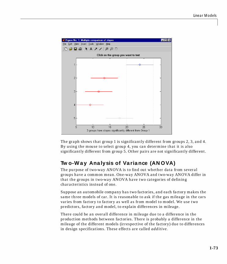
Linear Models
1-73
The graph shows that group 1 is significantly different from groups 2, 3, and 4.By using the mouse to select group 4, you can determine that it is alsosignificantly different from group 5. Other pairs are not significantly different.
Two-Way Analysis of Variance (ANOVA)The purpose of two-way ANOVA is to find out whether data from severalgroups have a common mean. One-way ANOVA and two-way ANOVA differ inthat the groups in two-way ANOVA have two categories of definingcharacteristics instead of one.
Suppose an automobile company has two factories, and each factory makes thesame three models of car. It is reasonable to ask if the gas mileage in the carsvaries from factory to factory as well as from model to model. We use twopredictors, factory and model, to explain differences in mileage.
There could be an overall difference in mileage due to a difference in theproduction methods between factories. There is probably a difference in themileage of the different models (irrespective of the factory) due to differencesin design specifications. These effects are called additive.

1 Tutorial
1-74
Finally, a factory might make high mileage cars in one model (perhaps becauseof a superior production line), but not be different from the other factory forother models. This effect is called an interaction. It is impossible to detect aninteraction unless there are duplicate observations for some combination offactory and car model.
Two-way ANOVA is a special case of the linear model. The two-way ANOVAform of the model is
where, with respect to the automobile example above:
• yijk is a matrix of gas mileage observations (with row index i, column index j,and repetition index k).
• µ is a constant matrix of the overall mean gas mileage.
• α.j is a matrix whose columns are the deviations of each car’s gas mileage(from the mean gas mileage µ) that are attributable to the car’s model. Allvalues in a given column of α.j are identical, and the values in each row of α.jsum to 0.
• βi. is a matrix whose rows are the deviations of each car’s gas mileage (fromthe mean gas mileage µ) that are attributable to the car’s factory. All valuesin a given row of βi. are identical, and the values in each column of βi. sumto 0.
• γij is a matrix of interactions. The values in each row of γij sum to 0, and thevalues in each column of γij sum to 0.
• εijk is a matrix of random disturbances.
The next section provides an example of a two-way analysis.
Example: Two-Way ANOVAThe purpose of the example is to determine the effect of car model and factoryon the mileage rating of cars.
load mileagemileage
yijk µ α.j βi . γij εijk+ + + +=

Linear Models
1-75
mileage =
33.3000 34.5000 37.4000 33.4000 34.8000 36.8000 32.9000 33.8000 37.6000 32.6000 33.4000 36.6000 32.5000 33.7000 37.0000 33.0000 33.9000 36.7000
cars = 3;[p,tbl,stats] = anova2(mileage,cars);p
p = 0.0000 0.0039 0.8411
There are three models of cars (columns) and two factories (rows). The reasonthere are six rows in mileage instead of two is that each factory provides threecars of each model for the study. The data from the first factory is in the firstthree rows, and the data from the second factory is in the last three rows.
The standard ANOVA table has columns for the sums of squares,degrees-of-freedom, mean squares (SS/df), F statistics, and p-values.
You can use the F statistics to do hypotheses tests to find out if the mileage isthe same across models, factories, and model-factory pairs (after adjusting forthe additive effects). anova2 returns the p-value from these tests.
The p-value for the model effect is zero to four decimal places. This is a strongindication that the mileage varies from one model to another. An F statistic asextreme as the observed F would occur by chance less than once in 10,000 timesif the gas mileage were truly equal from model to model. If you used the
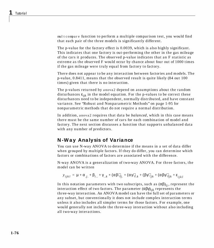
1 Tutorial
1-76
multcompare function to perform a multiple comparison test, you would findthat each pair of the three models is significantly different.
The p-value for the factory effect is 0.0039, which is also highly significant.This indicates that one factory is out-performing the other in the gas mileageof the cars it produces. The observed p-value indicates that an F statistic asextreme as the observed F would occur by chance about four out of 1000 timesif the gas mileage were truly equal from factory to factory.
There does not appear to be any interaction between factories and models. Thep-value, 0.8411, means that the observed result is quite likely (84 out 100times) given that there is no interaction.
The p-values returned by anova2 depend on assumptions about the randomdisturbances εijk in the model equation. For the p-values to be correct thesedisturbances need to be independent, normally distributed, and have constantvariance. See “Robust and Nonparametric Methods” on page 1-95 fornonparametric methods that do not require a normal distribution.
In addition, anova2 requires that data be balanced, which in this case meansthere must be the same number of cars for each combination of model andfactory. The next section discusses a function that supports unbalanced datawith any number of predictors.
N-Way Analysis of VarianceYou can use N-way ANOVA to determine if the means in a set of data differwhen grouped by multiple factors. If they do differ, you can determine whichfactors or combinations of factors are associated with the difference.
N-way ANOVA is a generalization of two-way ANOVA. For three factors, themodel can be written
In this notation parameters with two subscripts, such as (αβ)ij., represent theinteraction effect of two factors. The parameter (αβγ)ijk represents thethree-way interaction. An ANOVA model can have the full set of parameters orany subset, but conventionally it does not include complex interaction termsunless it also includes all simpler terms for those factors. For example, onewould generally not include the three-way interaction without also includingall two-way interactions.
yijkl µ α.j. βi . . γ..k αβ( )ij. αγ( )i .k βγ( ).jk αβγ( )ijk ε+ + + + ijkl+ + + +=

Linear Models
1-77
The anovan function performs N-way ANOVA. Unlike the anova1 and anova2functions, anovan does not expect data in a tabular form. Instead, it expects avector of response measurements and a separate vector (or text array)containing the values corresponding to each factor. This input data format ismore convenient than matrices when there are more than two factors or whenthe number of measurements per factor combination is not constant.
The following examples explore anovan in greater detail:
• “Example: N-Way ANOVA with Small Data Set”
• “Example: N-Way ANOVA with Large Data Set”
Example: N-Way ANOVA with Small Data SetConsider the following two-way example using anova2.
m = [23 15 20;27 17 63;43 3 55;41 9 90]m = 23 15 20 27 17 63 43 3 55 41 9 90
anova2(m,2)
ans = 0.0197 0.2234 0.2663
The factor information is implied by the shape of the matrix m and the numberof measurements at each factor combination (2). Although anova2 does notactually require arrays of factor values, for illustrative purposes we couldcreate them as follows.
cfactor = repmat(1:3,4,1)
cfactor =
1 2 3 1 2 3 1 2 3 1 2 3

1 Tutorial
1-78
rfactor = [ones(2,3); 2*ones(2,3)]
rfactor =
1 1 1 1 1 1 2 2 2 2 2 2
The cfactor matrix shows that each column of m represents a different level ofthe column factor. The rfactor matrix shows that the top two rows of mrepresent one level of the row factor, and bottom two rows of m represent asecond level of the row factor. In other words, each value m(i,j) represents anobservation at column factor level cfactor(i,j) and row factor levelcfactor(i,j).
To solve the above problem with anovan, we need to reshape the matrices m,cfactor, and rfactor to be vectors.
m = m(:);cfactor = cfactor(:);rfactor = rfactor(:);
[m cfactor rfactor]
ans =
23 1 1 27 1 1 43 1 2 41 1 2 15 2 1 17 2 1 3 2 2 9 2 2 20 3 1 63 3 1 55 3 2 90 3 2

Linear Models
1-79
anovan(m,{cfactor rfactor},2)
ans =
0.0197 0.2234 0.2663
Example: N-Way ANOVA with Large Data SetIn the previous example we used anova2 to study a small data set measuringcar mileage. Now we study a larger set of car data with mileage and otherinformation on 406 cars made between 1970 and 1982. First we load the dataset and look at the variable names.
load carbigwhos
Name Size Bytes Class
Acceleration 406x1 3248 double array Cylinders 406x1 3248 double array Displacement 406x1 3248 double array Horsepower 406x1 3248 double array MPG 406x1 3248 double array Model 406x36 29232 char array Model_Year 406x1 3248 double array Origin 406x7 5684 char array Weight 406x1 3248 double array cyl4 406x5 4060 char array org 406x7 5684 char array when 406x5 4060 char array
We will focus our attention on four variables. MPG is the number of miles pergallon for each of 406 cars (though some have missing values coded as NaN). Theother three variables are factors: cyl4 (four-cylinder car or not), org (caroriginated in Europe, Japan, or the USA), and when (car was built early in theperiod, in the middle of the period, or late in the period).

1 Tutorial
1-80
First we fit the full model, requesting up to three-way interactions and Type 3sums-of-squares.
varnames = {'Origin';'4Cyl';'MfgDate'};anovan(MPG,{org cyl4 when},3,3,varnames)
ans = 0.0000 NaN 0 0.7032 0.0001 0.2072 0.6990
Note that many terms are marked by a “#” symbol as not having full rank, andone of them has zero degrees of freedom and is missing a p-value. This canhappen when there are missing factor combinations and the model hashigher-order terms. In this case, the cross-tabulation below shows that thereare no cars made in Europe during the early part of the period with other thanfour cylinders, as indicated by the 0 in table(2,1,1).
[table,factorvals] = crosstab(org,when,cyl4)
table(:,:,1) =
82 75 25 0 4 3 3 3 4

Linear Models
1-81
table(:,:,2) =
12 22 38 23 26 17 12 25 32
factorvals =
'USA' 'Early' 'Other' 'Europe' 'Mid' 'Four' 'Japan' 'Late' []
Consequently it is impossible to estimate the three-way interaction effects, andincluding the three-way interaction term in the model makes the fit singular.
Using even the limited information available in the ANOVA table, we can seethat the three-way interaction has a p-value of 0.699, so it is not significant. Wedecide to request only two-way interactions this time.
[p,tbl,stats,termvec] = anovan(MPG,{org cyl4 when},2,3,varnames);termvec'
ans =
1 2 4 3 5 6
Now all terms are estimable. The p-values for interaction term 4(Origin*4Cyl) and interaction term 6 (4Cyl*MfgDate) are much larger than atypical cutoff value of 0.05, indicating these terms are not significant. We couldchoose to omit these terms and pool their effects into the error term. The outputtermvec variable returns a vector of codes, each of which is a bit patternrepresenting a term. We can omit terms from the model by deleting their
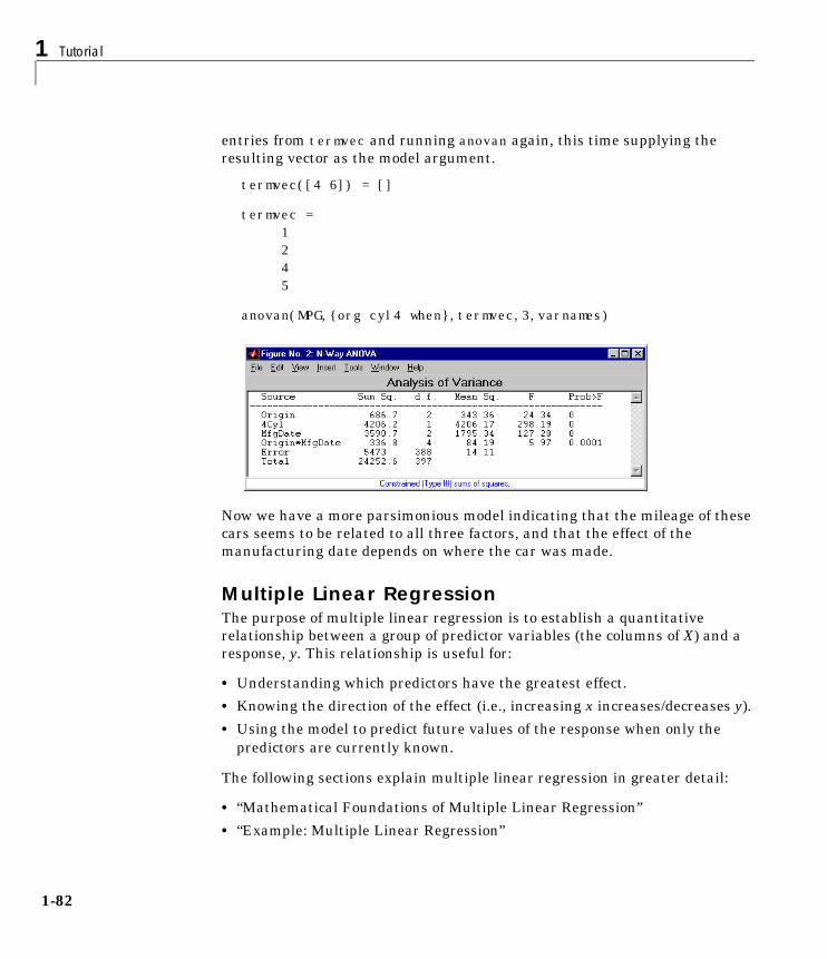
1 Tutorial
1-82
entries from termvec and running anovan again, this time supplying theresulting vector as the model argument.
termvec([4 6]) = []
termvec = 1 2 4 5
anovan(MPG,{org cyl4 when},termvec,3,varnames)
Now we have a more parsimonious model indicating that the mileage of thesecars seems to be related to all three factors, and that the effect of themanufacturing date depends on where the car was made.
Multiple Linear RegressionThe purpose of multiple linear regression is to establish a quantitativerelationship between a group of predictor variables (the columns of X) and aresponse, y. This relationship is useful for:
• Understanding which predictors have the greatest effect.
• Knowing the direction of the effect (i.e., increasing x increases/decreases y).
• Using the model to predict future values of the response when only thepredictors are currently known.
The following sections explain multiple linear regression in greater detail:
• “Mathematical Foundations of Multiple Linear Regression”
• “Example: Multiple Linear Regression”

Linear Models
1-83
Mathematical Foundations of Multiple Linear RegressionThe linear model takes its common form
where:
• y is an n-by-1 vector of observations.
• X is an n-by-p matrix of regressors.
• β is a p-by-1 vector of parameters.
• ε is an n-by-1 vector of random disturbances.
The solution to the problem is a vector, b, which estimates the unknown vectorof parameters, β. The least squares solution is
This equation is useful for developing later statistical formulas, but has poornumeric properties. regress uses QR decomposition of X followed by thebackslash operator to compute b. The QR decomposition is not necessary forcomputing b, but the matrix R is useful for computing confidence intervals.
You can plug b back into the model formula to get the predicted y values at thedata points.
Statisticians use a hat (circumflex) over a letter to denote an estimate of aparameter or a prediction from a model. The projection matrix H is called thehat matrix, because it puts the “hat” on y.
The residuals are the difference between the observed and predicted y values.
The residuals are useful for detecting failures in the model assumptions, sincethey correspond to the errors, ε, in the model equation. By assumption, theseerrors each have independent normal distributions with mean zero and aconstant variance.
y Xβ ε+=
b β XTX( )1–XTy= =
y Xb Hy= =
H X XTX( )1–XT
=
r y y–= I H–( )y=

1 Tutorial
1-84
The residuals, however, are correlated and have variances that depend on thelocations of the data points. It is a common practice to scale (“Studentize”) theresiduals so they all have the same variance.
In the equation below, the scaled residual, ti, has a Student’s t distributionwith (n-p-1) degrees of freedom
where
and:
• ti is the scaled residual for the ith data point.
• ri is the raw residual for the ith data point.
• n is the sample size.
• p is the number of parameters in the model.
• hi is the ith diagonal element of H.
The left-hand side of the second equation is the estimate of the variance of theerrors excluding the ith data point from the calculation.
A hypothesis test for outliers involves comparing ti with the critical values ofthe t distribution. If ti is large, this casts doubt on the assumption that thisresidual has the same variance as the others.
A confidence interval for the mean of each error is
Confidence intervals that do not include zero are equivalent to rejecting thehypothesis (at a significance probability of α) that the residual mean is zero.Such confidence intervals are good evidence that the observation is an outlierfor the given model.
ti
ri
σ i( ) 1 hi–----------------------------=
σ2
i( )r 2
n p– 1–----------------------
ri2
n p– 1–( ) 1 hi–( )-----------------------------------------------–=
ci ri t1 α
2--- ν,–
� �� �
± σ i( ) 1 hi–=

Linear Models
1-85
Example: Multiple Linear RegressionThe example comes from Chatterjee and Hadi (1986) in a paper on regressiondiagnostics. The data set (originally from Moore (1975)) has five predictorvariables and one response.
load mooreX = [ones(size(moore,1),1) moore(:,1:5)];
Matrix X has a column of ones, and then one column of values for each of thefive predictor variables. The column of ones is necessary for estimating they-intercept of the linear model.
y = moore(:,6);[b,bint,r,rint,stats] = regress(y,X);
The y-intercept is b(1), which corresponds to the column index of the columnof ones.
statsstats =
0.8107 11.9886 0.0001
The elements of the vector stats are the regression R2 statistic, the F statistic(for the hypothesis test that all the regression coefficients are zero), and thep-value associated with this F statistic.
R2 is 0.8107 indicating the model accounts for over 80% of the variability in theobservations. The F statistic of about 12 and its p-value of 0.0001 indicate thatit is highly unlikely that all of the regression coefficients are zero.
rcoplot(r,rint)
0 5 10 15 20
-0.5
0
0.5
Res
idua
ls
Case Number

1 Tutorial
1-86
The plot shows the residuals plotted in case order (by row). The 95% confidenceintervals about these residuals are plotted as error bars. The first observationis an outlier since its error bar does not cross the zero reference line.
In problems with just a single predictor, it is simpler to use the polytoolfunction (see “The polytool Demo” on page 1-156). This function can form anX matrix with predictor values, their squares, their cubes, and so on.
Quadratic Response Surface ModelsResponse Surface Methodology (RSM) is a tool for understanding thequantitative relationship between multiple input variables and one outputvariable.
Consider one output, z, as a polynomial function of two inputs, x and y. Thefunction z = f(x,y) describes a two-dimensional surface in the space (x,y,z). Ofcourse, you can have as many input variables as you want and the resultingsurface becomes a hypersurface. You can have multiple output variables witha separate hypersurface for each one.
For three inputs (x1, x2, x3), the equation of a quadratic response surface is
It is difficult to visualize a k-dimensional surface in k+1 dimensional spacefor k>2. The function rstool is a graphical user interface (GUI) designed tomake this visualization more intuitive, as is discussed in the next section.
Exploring Graphs of Multidimensional PolynomialsThe function rstool is useful for fitting response surface models. The purposeof rstool is larger than just fitting and prediction for polynomial models. ThisGUI provides an environment for exploration of the graph of amultidimensional polynomial.
You can learn about rstool by trying the commands below. The chemistrybehind the data in reaction.mat deals with reaction kinetics as a function of
y b0 b1x1 b2x2 b3x3 …
b12x1x2 b13x1x3 b23x2x3 …
b11x12 b22x2
2 b33x32
+ + + +
+ + + +
+ + +
= (linear terms)
(interaction terms)
(quadratic terms)

Linear Models
1-87
the partial pressure of three chemical reactants: hydrogen, n-pentane, andisopentane.
load reactionrstool(reactants,rate,'quadratic',0.01,xn,yn)
You will see a “vector” of three plots. The dependent variable of all three plotsis the reaction rate. The first plot has hydrogen as the independent variable.The second and third plots have n-pentane and isopentane respectively.
Each plot shows the fitted relationship of the reaction rate to the independentvariable at a fixed value of the other two independent variables. The fixedvalue of each independent variable is in an editable text box below each axis.You can change the fixed value of any independent variable by either typing anew value in the box or by dragging any of the three vertical lines to a newposition.
When you change the value of an independent variable, all the plots update toshow the current picture at the new point in the space of the independentvariables.
Note that while this example only uses three inputs (reactants) and one output(rate), rstool can accommodate an arbitrary number of inputs and outputs.Interpretability may be limited by the size of the monitor for large numbers ofinputs or outputs.
The GUI also has two pop-up menus. The Export menu facilitates savingvarious important variables in the GUI to the base workspace. Below theExport menu there is another menu that allows you to change the order of thepolynomial model from within the GUI. If you used the commands above, thismenu will have the string Full Quadratic. Other choices are:
• Linear – has the constant and first order terms only.
• Pure Quadratic – includes constant, linear and squared terms.
• Interactions – includes constant, linear, and cross product terms.
The rstool GUI is used by the rsmdemo function to visualize the results of adesigned experiment for studying a chemical reaction. See “The rsmdemoDemo” on page 1-170.

1 Tutorial
1-88
Stepwise Regression Stepwise regression is a technique for choosing the variables to include in amultiple regression model. Forward stepwise regression starts with no modelterms. At each step it adds the most statistically significant term (the one withthe highest F statistic or lowest p-value) until there are none left. Backwardstepwise regression starts with all the terms in the model and removes theleast significant terms until all the remaining terms are statisticallysignificant. It is also possible to start with a subset of all the terms and thenadd significant terms or remove insignificant terms.
An important assumption behind the method is that some input variables in amultiple regression do not have an important explanatory effect on theresponse. If this assumption is true, then it is a convenient simplification tokeep only the statistically significant terms in the model.
One common problem in multiple regression analysis is multicollinearity of theinput variables. The input variables may be as correlated with each other asthey are with the response. If this is the case, the presence of one input variablein the model may mask the effect of another input. Stepwise regression used asa canned procedure is a dangerous tool because the resulting model mayinclude different variables depending on the choice of starting model andinclusion strategy.
The following example explores an interactive tool for stepwise regression.
Example: Stepwise RegressionThe Statistics Toolbox provides an interactive graphical user interface (GUI) tomake comparison of competing models more understandable. You can explorethe GUI using the Hald (1960) data set. Here are the commands to get started.
load haldstepwise(ingredients,heat)
The Hald data come from a study of the heat of reaction of various cementmixtures. There are four components in each mixture, and the amount of heatproduced depends on the amount of each ingredient in the mixture.
Linear Models
1-89
The interface consists of three interactively linked figure windows. Two ofthese are discussed in the following sections:
• “Stepwise Regression Plot”
• “Stepwise Regression Diagnostics Table”
All three windows have hot regions. When your mouse is above one of theseregions, the pointer changes from an arrow to a circle. Clicking on this pointinitiates some activity in the interface.
Stepwise Regression PlotThis plot shows the regression coefficient and confidence interval for everyterm (in or out of the model). The green lines represent terms in the modelwhile red lines indicate terms that are not currently in the model.
Statistically significant terms are solid lines. Dotted lines show that the fittedcoefficient is not significantly different from zero.
Clicking on a line in this plot toggles its state. That is, a term currently in themodel (green line) is removed (turns red), and a term currently not in the model(red line) is added (turns green).
The coefficient for a term out of the model is the coefficient resulting fromadding that term to the current model.
Scale Inputs. Pressing this button centers and normalizes the columns of theinput matrix to have a standard deviation of one.
Export. This pop-up menu allows you to export variables from the stepwisefunction to the base workspace.
Close. The Close button removes all the figure windows.

1 Tutorial
1-90
Stepwise Regression Diagnostics TableThis table is a quantitative view of the information in the Stepwise RegressionPlot. The table shows the Hald model with the second and third terms removed.
Coefficients and Confidence Intervals. The table at the top of the figure shows theregression coefficient and confidence interval for every term (in or out of themodel.) The green rows in the table (on your monitor) represent terms in themodel while red rows indicate terms not currently in the model.
Clicking on a row in this table toggles the state of the corresponding term. Thatis, a term currently in the model (green row) is removed (turns red), and a termcurrently not in the model (red row) is added to the model (turns green).
The coefficient for a term out of the model is the coefficient resulting fromadding that term to the current model.
Additional Diagnostic Statistics. There are also several diagnostic statistics at thebottom of the table:
• RMSE – the root mean squared error of the current model.
• R-square – the amount of response variability explained by the model.
• F – the overall F statistic for the regression.
• P – the associated significance probability.
Close Button. Shuts down all windows.
Confidence Intervals
Column #
RMSE
Parameter
R-square
Lower
F
Upper
P
1 1.44 1.02 1.86
2.734 0.9725 176.6 1.581e-08
2 0.4161 -0.1602 0.9924
2.734 0.9725 176.6 1.581e-08
3 -0.41 -1.029 0.2086
2.734 0.9725 176.6 1.581e-08
4 -0.614 -0.7615 -0.4664
2.734 0.9725 176.6 1.581e-08
Linear Models
1-91
Help Button. Activates online help.
Stepwise History. This plot shows the RMSE and a confidence interval for everymodel generated in the course of the interactive use of the other windows.
Recreating a Previous Model. Clicking on one of these lines recreates the currentmodel at that point in the analysis using a new set of windows. You can thuscompare the two candidate models directly.
Generalized Linear ModelsSo far, the functions in this section have dealt with models that have a linearrelationship between the response and one or more predictors. Sometimes youmay have a nonlinear relationship instead. To fit nonlinear models you can usethe functions described in “Nonlinear Regression Models” on page 1-100.
There are some nonlinear models, known as generalized linear models, thatyou can fit using simpler linear methods. To understand generalized linearmodels, first let’s review the linear models we have seen so far. Each of thesemodels has the following three characteristics:
• The response has a normal distribution with mean µ.
• A coefficient vector b defines a linear combination X*b of the predictors X.
• The model equates the two as µ = X*b.
In generalized linear models, these characteristics are generalized as follows:
• The response has a distribution that may be normal, binomial, Poisson,gamma, or inverse Gaussian, with parameters including a mean µ.
• A coefficient vector b defines a linear combination X*b of the predictors X.
• A link function f(·) defines the link between the two as f(µ) = X*b.
The following example explores this in greater detail.
Example: Generalized Linear ModelsFor example, consider the following data derived from the carbig data set. Wehave cars of various weights, and we record the total number of cars of eachweight and the number qualifying as poor-mileage cars because their miles pergallon value is below some target. (Suppose we don’t know the miles per gallonfor each car, only the number passing the test.) It might be reasonable to

1 Tutorial
1-92
assume that the value of the variable poor follows a binomial distribution withparameter N=total and with a p parameter that depends on the car weight. Aplot shows that the proportion of poor-mileage cars follows a nonlinearS-shape.
w = [2100 2300 2500 2700 2900 3100 3300 3500 3700 3900 4100 4300]';poor = [1 2 0 3 8 8 14 17 19 15 17 21]';total = [48 42 31 34 31 21 23 23 21 16 17 21]';
[w poor total]ans = 2100 1 48 2300 2 42 2500 0 31 2700 3 34 2900 8 31 3100 8 21 3300 14 23 3500 17 23 3700 19 21 3900 15 16 4100 17 17 4300 21 21
plot(w,poor./total,'x')
2000 2500 3000 3500 4000 45000
0.1
0.2
0.3
0.4
0.5
0.6
0.7
0.8
0.9
1

Linear Models
1-93
This shape is typical of graphs of proportions, as they have natural boundariesat 0.0 and 1.0.
A linear regression model would not produce a satisfactory fit to this graph. Notonly would the fitted line not follow the data points, it would produce invalidproportions less than 0 for light cars, and higher than 1 for heavy cars.
There is a class of regression models for dealing with proportion data. Thelogistic model is one such model. It defines the relationship between proportionp and weight w to be
Is this a good model for our data? It would be helpful to graph the data on thisscale, to see if the relationship appears linear. However, some of ourproportions are 0 and 1, so we cannot explicitly evaluate the left-hand-side ofthe equation. A useful trick is to compute adjusted proportions by adding smallincrements to the poor and total values — say a half observation to poor anda full observation to total. This keeps the proportions within range. A graphnow shows a more nearly linear relationship.
padj = (poor+.5) ./ (total+1);plot(w,log(padj./(1-padj)),'x')
We can use the glmfit function to fit this logistic model.
p1 p–------------� �� �log b1 b2w+=
2000 2500 3000 3500 4000 4500−5
−4
−3
−2
−1
0
1
2
3
4

1 Tutorial
1-94
b = glmfit(w,[poor total],'binomial')
b = -13.3801 0.0042
To use these coefficients to compute a fitted proportion, we have to invert thelogistic relationship. Some simple algebra shows that the logistic equation canalso be written as
Fortunately, the function glmval can decode this link function to compute thefitted values. Using this function we can graph fitted proportions for a range ofcar weights, and superimpose this curve on the original scatter plot.
x = 2100:100:4500;y = glmval(b,x,’logit’);plot(w,poor./total,'x',x,y,'r-')
Generalized linear models can fit a variety of distributions with a variety ofrelationships between the distribution parameters and the predictors. A fulldescription is beyond the scope of this document. For more information seeDobson (1990), or McCullagh and Nelder (1990). Also see the referencematerial for glmfit.
p 11 b– 1 b2w–( )exp+---------------------------------------------------=
2000 2500 3000 3500 4000 45000
0.1
0.2
0.3
0.4
0.5
0.6
0.7
0.8
0.9
1

Linear Models
1-95
Robust and Nonparametric MethodsAs mentioned in the previous sections, regression and analysis of varianceprocedures depend on certain assumptions, such as a normal distribution forthe error term. Sometimes such an assumption is not warranted. For example,if the distribution of the errors is asymmetric or prone to extreme outliers, thatis a violation of the assumption of normal errors.
The Statistics Toolbox has a robust regression function that is useful whenthere may be outliers. Robust methods are designed to be relatively insensitiveto large changes in a small part of the data.
The Statistics Toolbox also has nonparametric versions of the one-way andtwo-way analysis of variance functions. Unlike classical tests, nonparametrictests make only mild assumptions about the data, and are appropriate whenthe distribution of the data is not normal. On the other hand, they are lesspowerful than classical methods for normally distributed data.
The following sections describe the robust regression and nonparametricfunctions in greater detail:
• “Robust Regression”
• “Kruskal-Wallis Test”
• “Friedman’s Test”
Both of the nonparametric functions described here can return a statsstructure that you can use as input to the multcompare function to performmultiple comparisons.
Robust RegressionIn “Example: Multiple Linear Regression” on page 1-85 we found an outlierwhen we used ordinary least squares regression to model a response as afunction of five predictors. How did that outlier affect the results?
Let’s estimate the coefficients using the robustfit function.
load moorex = moore(:,1:5);y = moore(:,6);[br,statsr] = robustfit(x,y);br

1 Tutorial
1-96
br = -1.7742 0.0000 0.0009 0.0002 0.0062 0.0001
Compare these estimates to those we obtained from the regress function.
bb = -2.1561 -0.0000 0.0013 0.0001 0.0079 0.0001
To understand why the two differ, it is helpful to look at the weight variablefrom the robust fit. It measures how much weight was given to each pointduring the fit. In this case, the first point had a very low weight so it waseffectively ignored.
statsr.w'
ans =
Columns 1 through 7 0.0577 0.9977 0.9776 0.9455 0.9687 0.8734 0.9177 Columns 8 through 14 0.9990 0.9653 0.9679 0.9768 0.9882 0.9998 0.9979 Columns 15 through 20 0.8185 0.9757 0.9875 0.9991 0.9021 0.6953
For another example illustrating robust fitting, see “The robustdemo Demo” onpage 1-172.

Linear Models
1-97
Kruskal-Wallis TestIn “One-Way Analysis of Variance (ANOVA)” on page 1-69 we used one-wayanalysis of variance to determine if the bacteria counts of milk varied fromshipment to shipment. Our one-way analysis rested on the assumption that themeasurements were independent, and that each had a normal distributionwith a common variance and with a mean that was constant in each column.We concluded that the column means were not all the same. Let’s repeat thatanalysis using a nonparametric procedure.
The Kruskal-Wallis test is a nonparametric version of one-way analysis ofvariance. The assumption behind this test is that the measurements come froma continuous distribution, but not necessarily a normal distribution. The testis based on an analysis of variance using the ranks of the data values, not thedata values themselves. Output includes a table similar to an anova table, anda box plot.
We can run this test as follows.
p = kruskalwallis(hogg)p = 0.0020
The low p-value means the Kruskal-Wallis test results agree with the one-wayanalysis of variance results.
Friedman’s TestIn “Two-Way Analysis of Variance (ANOVA)” on page 1-73 we used two-wayanalysis of variance to study the effect of car model and factory on car mileage.We tested whether either of these factors had a significant effect on mileage,and whether there was an interaction between these factors. We concludedthat there was no interaction, but that each individual factor had a significanteffect. Now we will see if a nonparametric analysis will lead to the sameconclusion.
Friedman’s test is a nonparametric test for data having a two-way layout (datagrouped by two categorical factors). Unlike two-way analysis of variance,Friedman’s test does not treat the two factors symmetrically and it does nottest for an interaction between them. Instead, it is a test for whether thecolumns are different after adjusting for possible row differences. The test isbased on an analysis of variance using the ranks of the data across categoriesof the row factor. Output includes a table similar to an anova table.
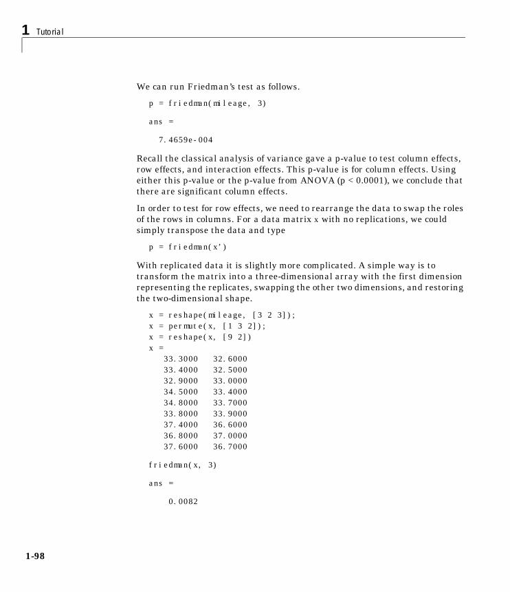
1 Tutorial
1-98
We can run Friedman’s test as follows.
p = friedman(mileage, 3)
ans =
7.4659e-004
Recall the classical analysis of variance gave a p-value to test column effects,row effects, and interaction effects. This p-value is for column effects. Usingeither this p-value or the p-value from ANOVA (p < 0.0001), we conclude thatthere are significant column effects.
In order to test for row effects, we need to rearrange the data to swap the rolesof the rows in columns. For a data matrix x with no replications, we couldsimply transpose the data and type
p = friedman(x’)
With replicated data it is slightly more complicated. A simple way is totransform the matrix into a three-dimensional array with the first dimensionrepresenting the replicates, swapping the other two dimensions, and restoringthe two-dimensional shape.
x = reshape(mileage, [3 2 3]);x = permute(x, [1 3 2]);x = reshape(x, [9 2])x = 33.3000 32.6000 33.4000 32.5000 32.9000 33.0000 34.5000 33.4000 34.8000 33.7000 33.8000 33.9000 37.4000 36.6000 36.8000 37.0000 37.6000 36.7000
friedman(x, 3)
ans =
0.0082

Linear Models
1-99
Again, the conclusion is similar to the conclusion from the classical analysis ofvariance. Both this p-value and the one from ANOVA (p = 0.0039) lead us toconclude there are significant row effects.
You cannot use Friedman’s test to test for interactions between the row andcolumn factors.

1 Tutorial
1-100
Nonlinear Regression ModelsResponse Surface Methodology (RSM) is an empirical modeling approach usingpolynomials as local approximations to the true input/output relationship. Thisempirical approach is often adequate for process improvement in an industrialsetting.
In scientific applications there is usually relevant theory that allows us tomake a mechanistic model. Often such models are nonlinear in the unknownparameters. Nonlinear models are more difficult to fit, requiring iterativemethods that start with an initial guess of the unknown parameters. Eachiteration alters the current guess until the algorithm converges.
The Statistics Toolbox has functions for fitting nonlinear models of the form
where:
• y is an-n by-1 vector of observations.
• f is any function of X and β.• X is an n-by-p matrix of input variables.
• β is a p-by-1 vector of unknown parameters to be estimated.
• ε is an n-by-1 vector of random disturbances.
This is explored further in the following example.
Example: Nonlinear ModelingThe Hougen-Watson model (Bates and Watts 1988) for reaction kinetics is onespecific example of this type. The form of the model is
where β1, β2, ..., β5 are the unknown parameters, and x1, x2, and x3 are thethree input variables. The three inputs are hydrogen, n-pentane, andisopentane. It is easy to see that the parameters do not enter the modellinearly.
y f X β,( ) ε+=
rateβ1 x2⋅ x3 β5⁄–
1 β2 x1⋅ β3 x2⋅ β4 x3⋅+ + +------------------------------------------------------------------------=
Nonlinear Regression Models
1-101
The file reaction.mat contains simulated data from this reaction.
load reactionwhoYour variables are:
beta rate xn model reactants yn
The variables are as follows:
• rate is a 13-by-1 vector of observed reaction rates.
• reactants is a 13-by-3 matrix of reactants.
• beta is 5-by-1 vector of initial parameter estimates.
• model is a string containing the nonlinear function name.
• xn is a string matrix of the names of the reactants.
• yn is a string containing the name of the response.
The data and model are explored further in the following sections:
• “Fitting the Hougen-Watson Model”
• “Confidence Intervals on the Parameter Estimates”
• “Confidence Intervals on the Predicted Responses”
• “An Interactive GUI for Nonlinear Fitting and Prediction”
Fitting the Hougen-Watson ModelThe Statistics Toolbox provides the function nlinfit for finding parameterestimates in nonlinear modeling. nlinfit returns the least squares parameterestimates. That is, it finds the parameters that minimize the sum of thesquared differences between the observed responses and their fitted values. Ituses the Gauss-Newton algorithm with Levenberg-Marquardt modificationsfor global convergence.
nlinfit requires the input data, the responses, and an initial guess of theunknown parameters. You must also supply the name of a function that takesthe input data and the current parameter estimate and returns the predictedresponses. In MATLAB terminology, nlinfit is called a “function” function.
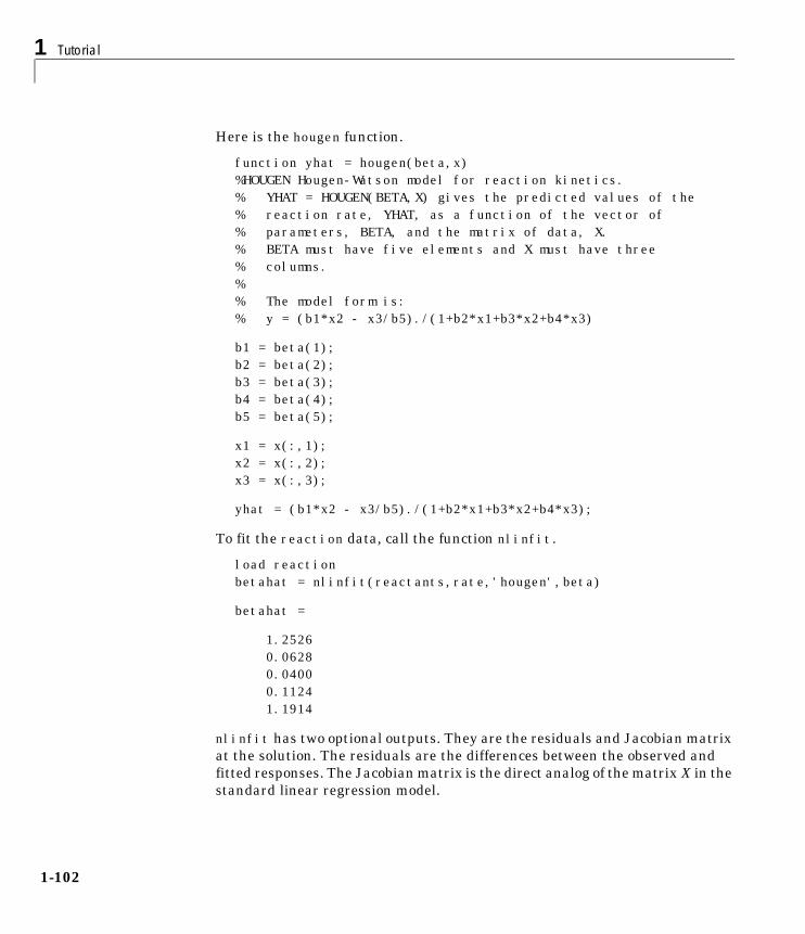
1 Tutorial
1-102
Here is the hougen function.
function yhat = hougen(beta,x)%HOUGEN Hougen-Watson model for reaction kinetics.% YHAT = HOUGEN(BETA,X) gives the predicted values of the% reaction rate, YHAT, as a function of the vector of % parameters, BETA, and the matrix of data, X.% BETA must have five elements and X must have three% columns.%% The model form is:% y = (b1*x2 - x3/b5)./(1+b2*x1+b3*x2+b4*x3)
b1 = beta(1);b2 = beta(2);b3 = beta(3);b4 = beta(4);b5 = beta(5);
x1 = x(:,1);x2 = x(:,2);x3 = x(:,3);
yhat = (b1*x2 - x3/b5)./(1+b2*x1+b3*x2+b4*x3);
To fit the reaction data, call the function nlinfit.
load reactionbetahat = nlinfit(reactants,rate,'hougen',beta)
betahat =
1.2526 0.0628 0.0400 0.1124 1.1914
nlinfit has two optional outputs. They are the residuals and Jacobian matrixat the solution. The residuals are the differences between the observed andfitted responses. The Jacobian matrix is the direct analog of the matrix X in thestandard linear regression model.

Nonlinear Regression Models
1-103
These outputs are useful for obtaining confidence intervals on the parameterestimates and predicted responses.
Confidence Intervals on the Parameter EstimatesUsing nlparci, form 95% confidence intervals on the parameter estimates,betahat, from the reaction kinetics example.
[betahat,resid,J] = nlinfit(reactants,rate,'hougen',beta);betaci = nlparci(betahat,resid,J)
betaci =
-0.7467 3.2519 -0.0377 0.1632 -0.0312 0.1113 -0.0609 0.2857 -0.7381 3.1208
Confidence Intervals on the Predicted ResponsesUsing nlpredci, form 95% confidence intervals on the predicted responsesfrom the reaction kinetics example.
[yhat,delta] = nlpredci('hougen',reactants,betahat,resid,J);opd = [rate yhat delta]
opd =
8.5500 8.2937 0.9178 3.7900 3.8584 0.7244 4.8200 4.7950 0.8267 0.0200 -0.0725 0.4775 2.7500 2.5687 0.4987 14.3900 14.2227 0.9666 2.5400 2.4393 0.9247 4.3500 3.9360 0.7327 13.0000 12.9440 0.7210 8.5000 8.2670 0.9459 0.0500 -0.1437 0.9537 11.3200 11.3484 0.9228 3.1300 3.3145 0.8418

1 Tutorial
1-104
Matrix opd has the observed rates in column 1 and the predictions in column 2.The 95% confidence interval is column 2±column 3. These are simultaneousconfidence intervals for the estimated function at each input value. They arenot intervals for new response observations at those inputs, even though mostof the confidence intervals do contain the original observations.
An Interactive GUI for Nonlinear Fitting and PredictionThe function nlintool for nonlinear models is a direct analog of rstool forpolynomial models. nlintool calls nlinfit and requires the same inputs.
The purpose of nlintool is larger than just fitting and prediction for nonlinearmodels. This GUI provides an environment for exploration of the graph of amultidimensional nonlinear function.
If you have already loaded reaction.mat, you can start nlintool.
nlintool(reactants,rate,'hougen',beta,0.01,xn,yn)
You will see a “vector” of three plots. The dependent variable of all three plotsis the reaction rate. The first plot has hydrogen as the independent variable.The second and third plots have n-pentane and isopentane respectively.
Each plot shows the fitted relationship of the reaction rate to the independentvariable at a fixed value of the other two independent variables. The fixedvalue of each independent variable is in an editable text box below each axis.You can change the fixed value of any independent variable by either typing anew value in the box or by dragging any of the three vertical lines to a newposition.
When you change the value of an independent variable, all the plots update toshow the current picture at the new point in the space of the independentvariables.
Note that while this example only uses three reactants, nlintool canaccommodate an arbitrary number of independent variables. Interpretabilitymay be limited by the size of the monitor for large numbers of inputs.

Hypothesis Tests
1-105
Hypothesis TestsA hypothesis test is a procedure for determining if an assertion about acharacteristic of a population is reasonable.
For example, suppose that someone says that the average price of a gallon ofregular unleaded gas in Massachusetts is $1.15. How would you decidewhether this statement is true? You could try to find out what every gas stationin the state was charging and how many gallons they were selling at that price.That approach might be definitive, but it could end up costing more than theinformation is worth.
A simpler approach is to find out the price of gas at a small number of randomlychosen stations around the state and compare the average price to $1.15.
Of course, the average price you get will probably not be exactly $1.15 due tovariability in price from one station to the next. Suppose your average pricewas $1.18. Is this three cent difference a result of chance variability, or is theoriginal assertion incorrect? A hypothesis test can provide an answer.
The following sections provide an overview of hypothesis testing with theStatistics Toolbox:
• “Hypothesis Test Terminology”
• “Hypothesis Test Assumptions”
• “Example: Hypothesis Testing”
• “Available Hypothesis Tests”
Hypothesis Test TerminologyTo get started, there are some terms to define and assumptions to make:
• The null hypothesis is the original assertion. In this case the null hypothesisis that the average price of a gallon of gas is $1.15. The notation isH0: µ = 1.15.
• There are three possibilities for the alternative hypothesis. You might only beinterested in the result if gas prices were actually higher. In this case, thealternative hypothesis is H1: µ > 1.15. The other possibilities are H1: µ < 1.15and H1: µ ≠ 1.15.
• The significance level is related to the degree of certainty you require in orderto reject the null hypothesis in favor of the alternative. By taking a small

1 Tutorial
1-106
sample you cannot be certain about your conclusion. So you decide inadvance to reject the null hypothesis if the probability of observing yoursampled result is less than the significance level. For a typical significancelevel of 5%, the notation is α = 0.05. For this significance level, theprobability of incorrectly rejecting the null hypothesis when it is actuallytrue is 5%. If you need more protection from this error, then choose a lowervalue of α.
• The p-value is the probability of observing the given sample result under theassumption that the null hypothesis is true. If the p-value is less than α, thenyou reject the null hypothesis. For example, if α = 0.05 and the p-value is0.03, then you reject the null hypothesis.
The converse is not true. If the p-value is greater than α, you haveinsufficient evidence to reject the null hypothesis.
• The outputs for many hypothesis test functions also include confidenceintervals. Loosely speaking, a confidence interval is a range of values thathave a chosen probability of containing the true hypothesized quantity.Suppose, in our example, 1.15 is inside a 95% confidence interval for themean, µ. That is equivalent to being unable to reject the null hypothesis at asignificance level of 0.05. Conversely if the 100(1-α) confidence interval doesnot contain 1.15, then you reject the null hypothesis at the α level ofsignificance.
Hypothesis Test AssumptionsThe difference between hypothesis test procedures often arises fromdifferences in the assumptions that the researcher is willing to make about thedata sample. For example, the Z-test assumes that the data representsindependent samples from the same normal distribution and that you know thestandard deviation, σ. The t-test has the same assumptions except that youestimate the standard deviation using the data instead of specifying it as aknown quantity.
Both tests have an associated signal-to-noise ratio
Z x µ–σ
------------ or T x µ–s
------------==
where xxin----
i 1=
n
�=

Hypothesis Tests
1-107
The signal is the difference between the average and the hypothesized mean.The noise is the standard deviation posited or estimated.
If the null hypothesis is true, then Z has a standard normal distribution,N(0,1). T has a Student’s t distribution with the degrees of freedom, ν, equal toone less than the number of data values.
Given the observed result for Z or T, and knowing the distribution of Z and Tassuming the null hypothesis is true, it is possible to compute the probability(p-value) of observing this result. A very small p-value casts doubt on the truthof the null hypothesis. For example, suppose that the p-value was 0.001,meaning that the probability of observing the given Z or T was one in athousand. That should make you skeptical enough about the null hypothesisthat you reject it rather than believe that your result was just a lucky 999 to 1shot.
There are also nonparametric tests that do not even require the assumptionthat the data come from a normal distribution. In addition, there are functionsfor testing whether the normal assumption is reasonable.
Example: Hypothesis TestingThis example uses the gasoline price data in gas.mat. There are two samplesof 20 observed gas prices for the months of January and February, 1993.
load gasprices = [price1 price2];
As a first step, you may want to test whether the samples from each monthfollow a normal distribution. As each sample is relatively small, you mightchoose to perform a Lilliefors test (rather than a Bera-Jarque test):
lillietest(price1)
ans =
0
lillietest(price2)
ans =
0

1 Tutorial
1-108
The result of the hypothesis test is a Boolean value that is 0 when you do notreject the null hypothesis, and 1 when you do reject that hypothesis. In eachcase, there is no need to reject the null hypothesis that the samples have anormal distribution.
Suppose it is historically true that the standard deviation of gas prices at gasstations around Massachusetts is four cents a gallon. The Z-test is a procedurefor testing the null hypothesis that the average price of a gallon of gas inJanuary (price1) is $1.15.
[h,pvalue,ci] = ztest(price1/100,1.15,0.04)
h = 0
pvalue =
0.8668
ci =
1.1340 1.1690
The Boolean output is h = 0, so you do not reject the null hypothesis.
The result suggests that $1.15 is reasonable. The 95% confidence interval[1.1340 1.1690] neatly brackets $1.15.
What about February? Try a t-test with price2. Now you are not assumingthat you know the standard deviation in price.
[h,pvalue,ci] = ttest(price2/100,1.15)
h = 1
pvalue =
4.9517e-04
ci = 1.1675 1.2025
With the Boolean result h = 1, you can reject the null hypothesis at the defaultsignificance level, 0.05.
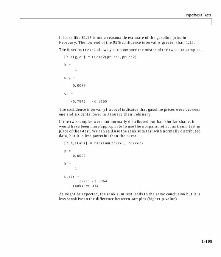
Hypothesis Tests
1-109
It looks like $1.15 is not a reasonable estimate of the gasoline price inFebruary. The low end of the 95% confidence interval is greater than 1.15.
The function ttest2 allows you to compare the means of the two data samples.
[h,sig,ci] = ttest2(price1,price2)
h = 1
sig =
0.0083
ci =
-5.7845 -0.9155
The confidence interval (ci above) indicates that gasoline prices were betweenone and six cents lower in January than February.
If the two samples were not normally distributed but had similar shape, itwould have been more appropriate to use the nonparametric rank sum test inplace of the t-test. We can still use the rank sum test with normally distributeddata, but it is less powerful than the t-test.
[p,h,stats] = ranksum(price1, price2)
p = 0.0092
h = 1
stats = zval: -2.6064 ranksum: 314
As might be expected, the rank sum test leads to the same conclusion but it isless sensitive to the difference between samples (higher p-value).

1 Tutorial
1-110
The box plot below gives the same conclusion graphically. Note that thenotches have little, if any, overlap. Refer to “Statistical Plots” on page 1-128 formore information about box plots.
boxplot(prices,1)set(gca,'XtickLabel',str2mat('January','February'))xlabel('Month')ylabel('Prices ($0.01)')
January February
110
115
120
125
Pric
es (
$0.0
1)
Month
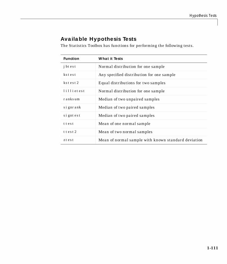
Hypothesis Tests
1-111
Available Hypothesis TestsThe Statistics Toolbox has functions for performing the following tests.
Function What it Tests
jbtest Normal distribution for one sample
kstest Any specified distribution for one sample
kstest2 Equal distributions for two samples
lillietest Normal distribution for one sample
ranksum Median of two unpaired samples
signrank Median of two paired samples
signtest Median of two paired samples
ttest Mean of one normal sample
ttest2 Mean of two normal samples
ztest Mean of normal sample with known standard deviation

1 Tutorial
1-112
Multivariate StatisticsMultivariate statistics is an omnibus term for a number of different statisticalmethods. The defining characteristic of these methods is that they all aim tounderstand a data set by considering a group of variables together rather thanfocusing on only one variable at a time.
The Statistics Toolbox has functions for principal components analysis(princomp), multivariate analysis of variance (manova1), and lineardiscriminant analysis (classify). The following sections illustrate the first twofunctions:
• “Principal Components Analysis”
• “Multivariate Analysis of Variance (MANOVA)”
Principal Components AnalysisOne of the difficulties inherent in multivariate statistics is the problem ofvisualizing multidimensionality. In MATLAB, the plot command displays agraph of the relationship between two variables. The plot3 and surfcommands display different three-dimensional views. When there are morethan three variables, it stretches the imagination to visualize theirrelationships.
Fortunately, in data sets with many variables, groups of variables often movetogether. One reason for this is that more than one variable may be measuringthe same driving principle governing the behavior of the system. In manysystems there are only a few such driving forces. But an abundance ofinstrumentation allows us to measure dozens of system variables. When thishappens, we can take advantage of this redundancy of information. We cansimplify our problem by replacing a group of variables with a single newvariable.
Principal components analysis is a quantitatively rigorous method forachieving this simplification. The method generates a new set of variables,called principal components. Each principal component is a linear combinationof the original variables. All the principal components are orthogonal to eachother so there is no redundant information. The principal components as awhole form an orthogonal basis for the space of the data.

Multivariate Statistics
1-113
There are an infinite number of ways to construct an orthogonal basis forseveral columns of data. What is so special about the principal componentbasis?
The first principal component is a single axis in space. When you project eachobservation on that axis, the resulting values form a new variable. And thevariance of this variable is the maximum among all possible choices of the firstaxis.
The second principal component is another axis in space, perpendicular to thefirst. Projecting the observations on this axis generates another new variable.The variance of this variable is the maximum among all possible choices of thissecond axis.
The full set of principal components is as large as the original set of variables.But it is commonplace for the sum of the variances of the first few principalcomponents to exceed 80% of the total variance of the original data. Byexamining plots of these few new variables, researchers often develop a deeperunderstanding of the driving forces that generated the original data.
The following section provides an example.
Example: Principal Components AnalysisLet us look at a sample application that uses nine different indices of thequality of life in 329 U.S. cities. These are climate, housing, health, crime,transportation, education, arts, recreation, and economics. For each index,higher is better; so, for example, a higher index for crime means a lower crimerate.
We start by loading the data in cities.mat.
load citieswhos
Name Size Bytes Class
categories 9x14 252 char array names 329x43 28294 char array ratings 329x9 23688 double array
The whos command generates a table of information about all the variables inthe workspace.

1 Tutorial
1-114
The cities data set contains three variables:
• categories, a string matrix containing the names of the indices.
• names, a string matrix containing the 329 city names.
• ratings, the data matrix with 329 rows and 9 columns.
Let’s look at the value of the categories variable.
categoriescategories =
climate housing health crime transportationeducation arts recreation economics
Now, let’s look at the first several rows of names variable.
first5 = names(1:5,:)first5 =
Abilene, TX Akron, OH Albany, GA Albany-Troy, NY Albuquerque, NM
To get a quick impression of the ratings data, make a box plot.
boxplot(ratings,0,'+',0)set(gca,'YTicklabel',categories)
These commands generate the plot below. Note that there is substantially morevariability in the ratings of the arts and housing than in the ratings of crimeand climate.

Multivariate Statistics
1-115
Ordinarily you might also graph pairs of the original variables, but there are36 two-variable plots. Perhaps principal components analysis can reduce thenumber of variables we need to consider.
Sometimes it makes sense to compute principal components for raw data. Thisis appropriate when all the variables are in the same units. Standardizing thedata is reasonable when the variables are in different units or when thevariance of the different columns is substantial (as in this case).
You can standardize the data by dividing each column by its standarddeviation.
stdr = std(ratings);sr = ratings./repmat(stdr,329,1);
Now we are ready to find the principal components.
[pcs,newdata,variances,t2] = princomp(sr);
The following sections explain the four outputs from princomp:
• “The Principal Components (First Output)”
• “The Component Scores (Second Output)”
• “The Component Variances (Third Output)”
• “Hotelling’s T2 (Fourth Output)”
0 1 2 3 4 5
x 104
climate
housing
health
crime
transportation
education
arts
recreation
economics
Values
Col
umn
Num
ber

1 Tutorial
1-116
The Principal Components (First Output)The first output of the princomp function, pcs, contains the nine principalcomponents. These are the linear combinations of the original variables thatgenerate the new variables.
Let’s look at the first three principal component vectors.
p3 = pcs(:,1:3)p3 =
0.2064 0.2178 -0.6900 0.3565 0.2506 -0.2082 0.4602 -0.2995 -0.0073 0.2813 0.3553 0.1851 0.3512 -0.1796 0.1464 0.2753 -0.4834 0.2297 0.4631 -0.1948 -0.0265 0.3279 0.3845 -0.0509 0.1354 0.4713 0.6073
The largest weights in the first column (first principal component) are the thirdand seventh elements, corresponding to the variables health and arts. All theelements of the first principal component are the same sign, making it aweighted average of all the variables.
To show the orthogonality of the principal components, note thatpremultiplying them by their transpose yields the identity matrix.
I = p3'*p3I =
1.0000 -0.0000 -0.0000 -0.0000 1.0000 -0.0000 -0.0000 -0.0000 1.0000

Multivariate Statistics
1-117
The Component Scores (Second Output)The second output, newdata, is the data in the new coordinate system definedby the principal components. This output is the same size as the input datamatrix.
A plot of the first two columns of newdata shows the ratings data projected ontothe first two principal components.
plot(newdata(:,1),newdata(:,2),'+')xlabel('1st Principal Component');ylabel('2nd Principal Component');
Note the outlying points in the lower right corner.
The function gname is useful for graphically identifying a few points in a plotlike this. You can call gname with a string matrix containing as many caselabels as points in the plot. The string matrix names works for labeling pointswith the city names.
gname(names)
Move your cursor over the plot and click once near each point at the top right.As you click on each point, MATLAB labels it with the proper row from thenames string matrix. When you are finished labeling points, press the Returnkey.
−4 −2 0 2 4 6 8 10 12 14−4
−3
−2
−1
0
1
2
3
4
1st Principal Component
2nd
Prin
cipa
l Com
pone
nt
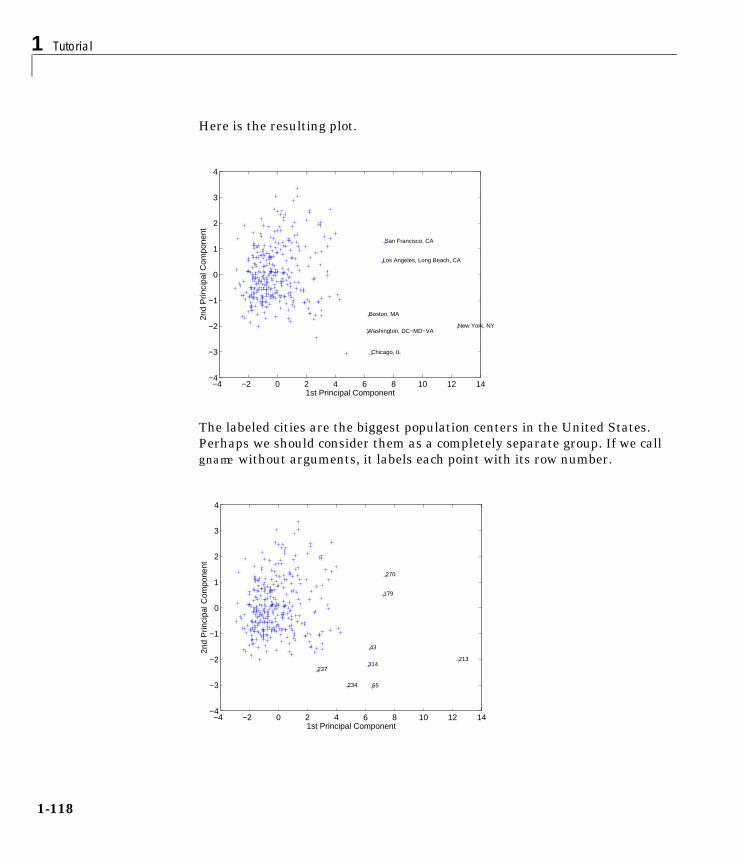
1 Tutorial
1-118
Here is the resulting plot.
The labeled cities are the biggest population centers in the United States.Perhaps we should consider them as a completely separate group. If we callgname without arguments, it labels each point with its row number.
−4 −2 0 2 4 6 8 10 12 14−4
−3
−2
−1
0
1
2
3
4
1st Principal Component
2nd
Prin
cipa
l Com
pone
nt
New York, NY
Los Angeles, Long Beach, CA
San Francisco, CA
Boston, MA
Washington, DC−MD−VA
Chicago, IL
−4 −2 0 2 4 6 8 10 12 14−4
−3
−2
−1
0
1
2
3
4
1st Principal Component
2nd
Prin
cipa
l Com
pone
nt
213
179
270
43
314
65
237
234

Multivariate Statistics
1-119
We can create an index variable containing the row numbers of all themetropolitan areas we chose.
metro = [43 65 179 213 234 270 314];names(metro,:)
ans =
Boston, MA Chicago, IL Los Angeles, Long Beach, CA New York, NY Philadelphia, PA-NJ San Francisco, CA Washington, DC-MD-VA
To remove these rows from the ratings matrix, type the following.
rsubset = ratings;nsubset = names;nsubset(metro,:) = [];rsubset(metro,:) = [];
size(rsubset)ans =
322 9
To practice, repeat the analysis using the variable rsubset as the new datamatrix and nsubset as the string matrix of labels.

1 Tutorial
1-120
The Component Variances (Third Output)The third output, variances, is a vector containing the variance explained bythe corresponding column of newdata.
variancesvariances =
3.4083 1.2140 1.1415 0.9209 0.7533 0.6306 0.4930 0.3180 0.1204
You can easily calculate the percent of the total variability explained by eachprincipal component.
percent_explained = 100*variances/sum(variances)percent_explained =
37.8699 13.4886 12.6831 10.2324 8.3698 7.0062 5.4783 3.5338 1.3378
A “Scree” plot is a pareto plot of the percent variability explained by eachprincipal component.
pareto(percent_explained)xlabel('Principal Component')ylabel('Variance Explained (%)')

Multivariate Statistics
1-121
We can see that the first three principal components explain roughly two thirdsof the total variability in the standardized ratings.
Hotelling’s T2 (Fourth Output)The last output of the princomp function, t2, is Hotelling’s T2, a statisticalmeasure of the multivariate distance of each observation from the center of thedata set. This is an analytical way to find the most extreme points in the data.
[st2, index] = sort(t2); % Sort in ascending order.st2 = flipud(st2); % Values in descending order.index = flipud(index); % Indices in descending order.
extreme = index(1)extreme =
213
names(extreme,:)ans =
New York, NY
It is not surprising that the ratings for New York are the furthest from theaverage U.S. town.
1 2 3 4 5 6 70
10
20
30
40
50
60
70
80
90
100
Principal Component
Var
ianc
e E
xpla
ined
(%
)
0%
10%
20%
30%
40%
50%
60%
70%
80%
90%
100%

1 Tutorial
1-122
Multivariate Analysis of Variance (MANOVA)We reviewed the analysis of variance technique in “One-Way Analysis ofVariance (ANOVA)” on page 1-69. With this technique we can take a set ofgrouped data and determine whether the mean of a variable differssignificantly between groups. Often we have multiple variables, and we areinterested in determining whether the entire set of means is different from onegroup to the next. There is a multivariate version of analysis of variance thatcan address that problem, as illustrated in the following example.
Example: Multivariate Analysis of VarianceThe carsmall data set has measurements on a variety of car models from theyears 1970, 1976, and 1982. Suppose we are interested in whether thecharacteristics of the cars have changed over time.
First we load the data.
load carsmallwhos
Name Size Bytes Class
Acceleration 100x1 800 double array Cylinders 100x1 800 double array Displacement 100x1 800 double array Horsepower 100x1 800 double array MPG 100x1 800 double array Model 100x36 7200 char array Model_Year 100x1 800 double array Origin 100x7 1400 char array Weight 100x1 800 double array
Four of these variables (Acceleration, Displacement, Horsepower, and MPG)are continuous measurements on individual car models. The variableModel_Year indicates the year in which the car was made. We can create agrouped plot matrix of these variables using the gplotmatrix function.
x = [MPG Horsepower Displacement Weight];gplotmatrix(x,[],Model_Year,[],'+xo')

Multivariate Statistics
1-123
(When the second argument of gplotmatrix is empty, the function graphs thecolumns of the x argument against each other, and places histograms along thediagonals. The empty fourth argument produces a graph with the defaultcolors. The fifth argument controls the symbols used to distinguish betweengroups.)
It appears the cars do differ from year to year. The upper right plot, forexample, is a graph of MPG versus Weight. The 1982 cars appear to have highermileage than the older cars, and they appear to weigh less on average. But asa group, are the three years significantly different from one another? Themanova1 function can answer that question.
[d,p,stats] = manova1(x,Model_Year)
d = 2
p =
1.0e-006 * 0 0.1141
2000 3000 4000200 400100 20020 402000
3000
4000
100
200
300
400
10
20
30
40
50
100
150
200
707682

1 Tutorial
1-124
stats = W: [4x4 double] B: [4x4 double] T: [4x4 double] dfW: 90 dfB: 2 dfT: 92 lambda: [2x1 double] chisq: [2x1 double] chisqdf: [2x1 double] eigenval: [4x1 double] eigenvec: [4x4 double] canon: [100x4 double] mdist: [100x1 double] gmdist: [3x3 double]
The manova1 function produces three outputs:
• The first output, d, is an estimate of the dimension of the group means. If themeans were all the same, the dimension would be 0, indicating that themeans are at the same point. If the means differed but fell along a line, thedimension would be 1. In the example the dimension is 2, indicating that thegroup means fall in a plane but not along a line. This is the largest possibledimension for the means of three groups.
• The second output, p, is a vector of p-values for a sequence of tests. The firstp-value tests whether the dimension is 0, the next whether the dimensionis 1, and so on. In this case both p-values are small. That’s why the estimateddimension is 2.
• The third output, stats, is a structure containing several fields, described inthe following section.
The Fields of the stats Structure. The W, B, and T fields are matrix analogs to thewithin, between, and total sums of squares in ordinary one-way analysis ofvariance. The next three fields are the degrees of freedom for these matrices.Fields lambda, chisq, and chisqdf are the ingredients of the test for thedimensionality of the group means. (The p-values for these tests are the firstoutput argument of manova1.)
The next three fields are used to do a canonical analysis. Recall that inprincipal components analysis (“Principal Components Analysis” on

Multivariate Statistics
1-125
page 1-112) we look for the combination of the original variables that has thelargest possible variation. In multivariate analysis of variance, we instead lookfor the linear combination of the original variables that has the largestseparation between groups. It is the single variable that would give the mostsignificant result in a univariate one-way analysis of variance. Having foundthat combination, we next look for the combination with the second highestseparation, and so on.
The eigenvec field is a matrix that defines the coefficients of the linearcombinations of the original variables. The eigenval field is a vectormeasuring the ratio of the between-group variance to the within-groupvariance for the corresponding linear combination. The canon field is a matrixof the canonical variable values. Each column is a linear combination of themean-centered original variables, using coefficients from the eigenvec matrix.
A grouped scatter plot of the first two canonical variables shows moreseparation between groups then a grouped scatter plot of any pair of originalvariables. In this example it shows three clouds of points, overlapping but withdistinct centers. One point in the bottom right sits apart from the others. Byusing the gname function, we can see that this is the 20th point.
c1 = stats.canon(:,1);c2 = stats.canon(:,2);gscatter(c2,c1,Model_Year,[],'oxs')gname
−4 −3 −2 −1 0 1 2 3 4 5−6
−4
−2
0
2
4
6
c2
c1
20
707682
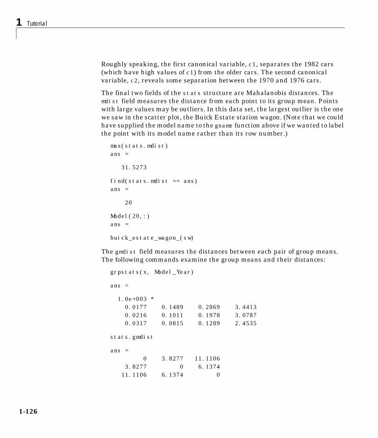
1 Tutorial
1-126
Roughly speaking, the first canonical variable, c1, separates the 1982 cars(which have high values of c1) from the older cars. The second canonicalvariable, c2, reveals some separation between the 1970 and 1976 cars.
The final two fields of the stats structure are Mahalanobis distances. Themdist field measures the distance from each point to its group mean. Pointswith large values may be outliers. In this data set, the largest outlier is the onewe saw in the scatter plot, the Buick Estate station wagon. (Note that we couldhave supplied the model name to the gname function above if we wanted to labelthe point with its model name rather than its row number.)
max(stats.mdist)ans =
31.5273
find(stats.mdist == ans)ans =
20
Model(20,:)ans =
buick_estate_wagon_(sw)
The gmdist field measures the distances between each pair of group means.The following commands examine the group means and their distances:
grpstats(x, Model_Year)
ans =
1.0e+003 * 0.0177 0.1489 0.2869 3.4413 0.0216 0.1011 0.1978 3.0787 0.0317 0.0815 0.1289 2.4535
stats.gmdist
ans = 0 3.8277 11.1106 3.8277 0 6.1374 11.1106 6.1374 0

Multivariate Statistics
1-127
As might be expected, the multivariate distance between the extreme years1970 and 1982 (11.1) is larger than the difference between more closely spacedyears (3.8 and 6.1). This is consistent with the scatter plots, where the pointsseem to follow a progression as the year changes from 1970 through 1976 to1982. If we had more groups, we might have found it instructive to use themanovacluster function to draw a diagram that presents clusters of thegroups, formed using the distances between their means.

1 Tutorial
1-128
Statistical PlotsThe Statistics Toolbox adds specialized plots to the extensive graphicscapabilities of MATLAB.
• Box plots are graphs for describing data samples. They are also useful forgraphic comparisons of the means of many samples (see “One-Way Analysisof Variance (ANOVA)” on page 1-69).
• Distribution plots are graphs for visualizing the distribution of one or moresamples. They include normal and Weibull probability plots,quantile-quantile plots, and empirical cumulative distribution plots.
• Scatter plots are graphs for visualizing the relationship between a pair ofvariables or several such pairs. Grouped versions of these plots use differentplotting symbols to indicate group membership. The gname function can labelpoints on these plots with a text label or an observation number.
The plot types are described further in the following sections:
• “Box Plots”
• “Distribution Plots”
• “Scatter Plots”
Box PlotsThe graph shows an example of a notched box plot.
1
110
115
120
125
Val
ues
Column Number

Statistical Plots
1-129
This plot has several graphic elements:
• The lower and upper lines of the “box” are the 25th and 75th percentiles ofthe sample. The distance between the top and bottom of the box is theinterquartile range.
• The line in the middle of the box is the sample median. If the median is notcentered in the box, that is an indication of skewness.
• The “whiskers” are lines extending above and below the box. They show theextent of the rest of the sample (unless there are outliers). Assuming nooutliers, the maximum of the sample is the top of the upper whisker. Theminimum of the sample is the bottom of the lower whisker. By default, anoutlier is a value that is more than 1.5 times the interquartile range awayfrom the top or bottom of the box.
• The plus sign at the top of the plot is an indication of an outlier in the data.This point may be the result of a data entry error, a poor measurement or achange in the system that generated the data.
• The notches in the box are a graphic confidence interval about the median ofa sample. Box plots do not have notches by default.
A side-by-side comparison of two notched box plots is the graphical equivalentof a t-test. See “Hypothesis Tests” on page 1-105.
Distribution PlotsThere are several types of plots for examining the distribution of one or moresamples, as described in the following sections:
• “Normal Probability Plots”
• “Quantile-Quantile Plots”
• “Weibull Probability Plots”
• “Empirical Cumulative Distribution Function (CDF)”
Normal Probability PlotsA normal probability plot is a useful graph for assessing whether data comesfrom a normal distribution. Many statistical procedures make the assumptionthat the underlying distribution of the data is normal, so this plot can providesome assurance that the assumption of normality is not being violated, orprovide an early warning of a problem with your assumptions.

1 Tutorial
1-130
This example shows a typical normal probability plot.
x = normrnd(10,1,25,1);normplot(x)
The plot has three graphical elements. The plus signs show the empiricalprobability versus the data value for each point in the sample. The solid lineconnects the 25th and 75th percentiles of the data and represents a robustlinear fit (i.e., insensitive to the extremes of the sample). The dashed lineextends the solid line to the ends of the sample.
The scale of the y-axis is not uniform. The y-axis values are probabilities and,as such, go from zero to one. The distance between the tick marks on the y-axismatches the distance between the quantiles of a normal distribution. Thequantiles are close together near the median (probability = 0.5) and stretch outsymmetrically moving away from the median. Compare the vertical distancefrom the bottom of the plot to the probability 0.25 with the distance from 0.25to 0.50. Similarly, compare the distance from the top of the plot to theprobability 0.75 with the distance from 0.75 to 0.50.
8.5 9 9.5 10 10.5 11 11.50.01 0.02
0.05
0.10
0.25
0.50
0.75
0.90
0.95
0.98 0.99
Data
Pro
babi
lity
Normal Probability Plot
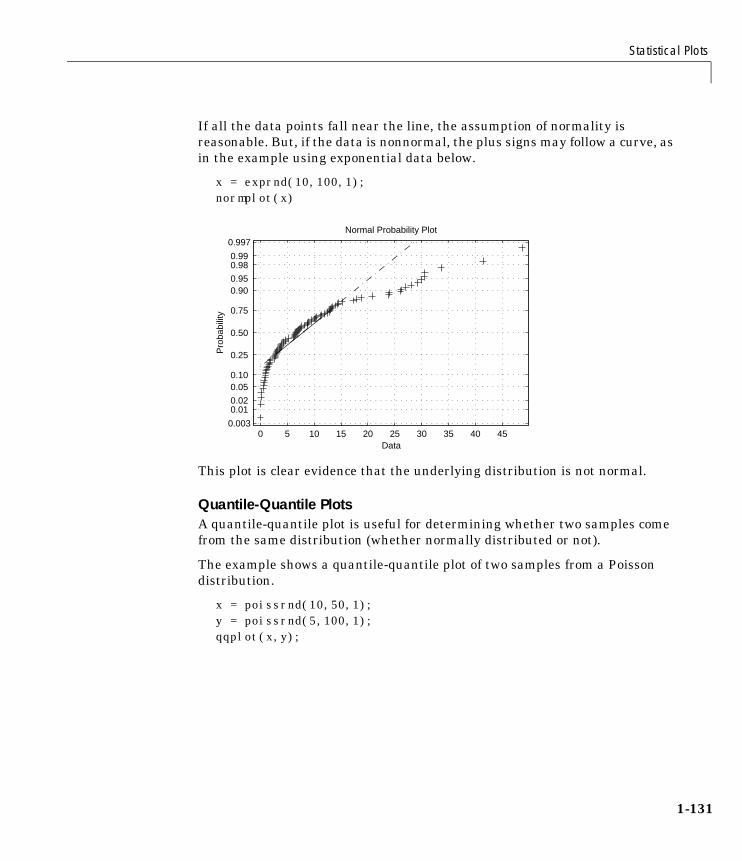
Statistical Plots
1-131
If all the data points fall near the line, the assumption of normality isreasonable. But, if the data is nonnormal, the plus signs may follow a curve, asin the example using exponential data below.
x = exprnd(10,100,1);normplot(x)
This plot is clear evidence that the underlying distribution is not normal.
Quantile-Quantile PlotsA quantile-quantile plot is useful for determining whether two samples comefrom the same distribution (whether normally distributed or not).
The example shows a quantile-quantile plot of two samples from a Poissondistribution.
x = poissrnd(10,50,1);y = poissrnd(5,100,1);qqplot(x,y);
0 5 10 15 20 25 30 35 40 450.003
0.01 0.02
0.05 0.10
0.25
0.50
0.75
0.90 0.95
0.98 0.99
0.997
Data
Pro
babi
lity
Normal Probability Plot

1 Tutorial
1-132
Even though the parameters and sample sizes are different, the straight linerelationship shows that the two samples come from the same distribution.
Like the normal probability plot, the quantile-quantile plot has three graphicalelements. The pluses are the quantiles of each sample. By default the numberof pluses is the number of data values in the smaller sample. The solid line joinsthe 25th and 75th percentiles of the samples. The dashed line extends the solidline to the extent of the sample.
The example below shows what happens when the underlying distributions arenot the same.
x = normrnd(5,1,100,1);y = weibrnd(2,0.5,100,1);qqplot(x,y);
2 4 6 8 10 12 14 16 18-2
0
2
4
6
8
10
12
X Quantiles
Y Q
uant
iles
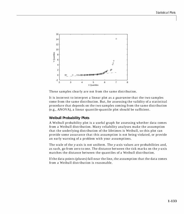
Statistical Plots
1-133
These samples clearly are not from the same distribution.
It is incorrect to interpret a linear plot as a guarantee that the two samplescome from the same distribution. But, for assessing the validity of a statisticalprocedure that depends on the two samples coming from the same distribution(e.g., ANOVA), a linear quantile-quantile plot should be sufficient.
Weibull Probability PlotsA Weibull probability plot is a useful graph for assessing whether data comesfrom a Weibull distribution. Many reliability analyses make the assumptionthat the underlying distribution of the lifetimes is Weibull, so this plot canprovide some assurance that this assumption is not being violated, or providean early warning of a problem with your assumptions.
The scale of the y-axis is not uniform. The y-axis values are probabilities and,as such, go from zero to one. The distance between the tick marks on the y-axismatches the distance between the quantiles of a Weibull distribution.
If the data points (pluses) fall near the line, the assumption that the data comesfrom a Weibull distribution is reasonable.
2 3 4 5 6 7 8-2
0
2
4
6
8
10
12
14
16
X Quantiles
Y Q
uant
iles

1 Tutorial
1-134
This example shows a typical Weibull probability plot.
y = weibrnd(2,0.5,100,1);weibplot(y)
Empirical Cumulative Distribution Function (CDF)If you are not willing to assume that your data follows a specific probabilitydistribution, you can use the cdfplot function to graph an empirical estimateof the cumulative distribution function (cdf). This function computes theproportion of data points less than each x value, and plots the proportion as afunction of x. The y-axis scale is linear, not a probability scale for a specificdistribution.
This example shows the empirical cumulative distribution function for aWeibull sample.
y = weibrnd(2,0.5,100,1);cdfplot(y)
10-4 10-2 100
0.003
0.01
0.02
0.05
0.10
0.25
0.50
0.75 0.90 0.96 0.99
Data
Pro
babi
lity
Weibull Probability Plot

Statistical Plots
1-135
The plot shows a probability function that rises steeply near x=0 and levels offfor larger values. Over 80% of the observations are less than 1, with theremaining values spread over the range [1 5].
Scatter PlotsA scatter plot is a simple plot of one variable against another. The MATLABplot and scatter functions can produce scatter plots. The MATLABplotmatrix function can produce a matrix of such plots showing therelationship between several pairs of variables.
The Statistics Toolbox adds functions that produce grouped versions of theseplots. These are useful for determining whether the values of two variables orthe relationship between those variables is the same in each group.
Suppose we want to examine the weight and mileage of cars from threedifferent model years.
load carsmallgscatter(Weight,MPG,Model_Year,'','xos')
0 1 2 3 4 50
0.1
0.2
0.3
0.4
0.5
0.6
0.7
0.8
0.9
1
x
F(x
)
Empirical CDF

1 Tutorial
1-136
This shows that not only is there a strong relationship between the weight of acar and its mileage, but also that newer cars tend to be lighter and have bettergas mileage than older cars.
(The default arguments for gscatter produce a scatter plot with the differentgroups shown with the same symbol but different colors. The last twoarguments above request that all groups be shown in default colors and withdifferent symbols.)
The carsmall data set contains other variables that describe different aspectsof cars. We can examine several of them in a single display by creating agrouped plot matrix.
xvars = [Weight Displacement Horsepower];yvars = [MPG Acceleration];gplotmatrix(xvars,yvars,Model_Year,'','xos')
1500 2000 2500 3000 3500 4000 4500 50005
10
15
20
25
30
35
40
45
Weight
MP
G
707682

Statistical Plots
1-137
The upper right subplot displays MPG against Horsepower, and shows that overthe years the horsepower of the cars has decreased but the gas mileage hasimproved.
The gplotmatrix function can also graph all pairs from a single list ofvariables, along with histograms for each variable. See “Multivariate Analysisof Variance (MANOVA)” on page 1-122.
50 100 150 200100 200 300 4002000 3000 4000
10
15
20
2510
20
30
40
707682

1 Tutorial
1-138
Statistical Process Control (SPC)SPC is an omnibus term for a number of methods for assessing and monitoringthe quality of manufactured goods. These methods are simple, which makesthem easy to implement even in a production environment. The followingsections discuss some of the SPC features of the Statistics Toolbox:
• “Control Charts”
• “Capability Studies”
Control ChartsThese graphs were popularized by Walter Shewhart in his work in the 1920sat Western Electric. A control chart is a plot of a measurements over time withstatistical limits applied. Actually, control chart is a slight misnomer. Thechart itself is actually a monitoring tool. The control activity may occur if thechart indicates that the process is changing in an undesirable systematicdirection.
The Statistics Toolbox supports three common control charts, described in thefollowing sections:
• “Xbar Charts”
• “S Charts”
• “EWMA Charts”
Xbar ChartsXbar charts are a plot of the average of a sample of a process taken at regularintervals. Suppose we are manufacturing pistons to a tolerance of0.5 thousandths of an inch. We measure the runout (deviation from circularityin thousandths of an inch) at four points on each piston.
load partsconf = 0.99;spec = [-0.5 0.5];xbarplot(runout,conf,spec)

Statistical Process Control (SPC)
1-139
The lines at the bottom and the top of the plot show the process specifications.The central line is the average runout over all the pistons. The two linesflanking the center line are the 99% statistical control limits. By chance onlyone measurement in 100 should fall outside these lines. We can see that evenin this small run of 36 parts, there are several points outside the boundaries(labeled by their observation numbers). This is an indication that the processmean is not in statistical control. This might not be of much concern in practice,since all the parts are well within specification.
S ChartsThe S chart is a plot of the standard deviation of a process taken at regularintervals. The standard deviation is a measure of the variability of a process.So, the plot indicates whether there is any systematic change in the processvariability. Continuing with the piston manufacturing example, we can look atthe standard deviation of each set of four measurements of runout.
schart(runout)
0 10 20 30 40
-0.4
-0.2
0
0.2
0.4
0.6
12
21 2526
30
Xbar Chart
USL
LSL
Samples
Mea
sure
men
tsLCL
UCL
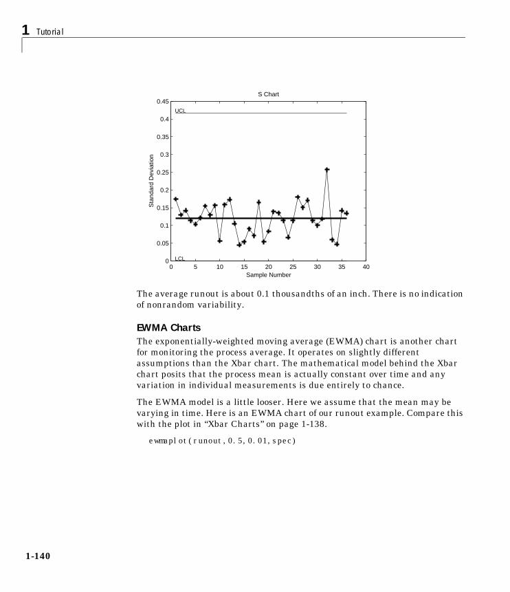
1 Tutorial
1-140
The average runout is about 0.1 thousandths of an inch. There is no indicationof nonrandom variability.
EWMA ChartsThe exponentially-weighted moving average (EWMA) chart is another chartfor monitoring the process average. It operates on slightly differentassumptions than the Xbar chart. The mathematical model behind the Xbarchart posits that the process mean is actually constant over time and anyvariation in individual measurements is due entirely to chance.
The EWMA model is a little looser. Here we assume that the mean may bevarying in time. Here is an EWMA chart of our runout example. Compare thiswith the plot in “Xbar Charts” on page 1-138.
ewmaplot(runout,0.5,0.01,spec)
0 5 10 15 20 25 30 35 400
0.05
0.1
0.15
0.2
0.25
0.3
0.35
0.4
0.45S Chart
Sample Number
Sta
ndar
d D
evia
tion
UCL
LCL
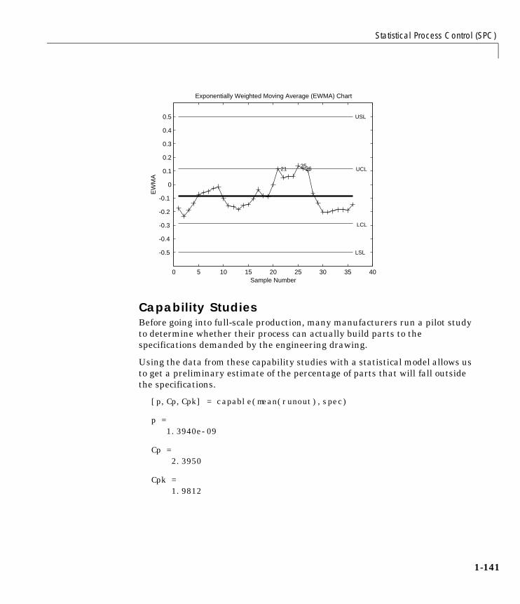
Statistical Process Control (SPC)
1-141
Capability StudiesBefore going into full-scale production, many manufacturers run a pilot studyto determine whether their process can actually build parts to thespecifications demanded by the engineering drawing.
Using the data from these capability studies with a statistical model allows usto get a preliminary estimate of the percentage of parts that will fall outsidethe specifications.
[p,Cp,Cpk] = capable(mean(runout),spec)
p = 1.3940e-09
Cp = 2.3950
Cpk = 1.9812
0 5 10 15 20 25 30 35 40
-0.5
-0.4
-0.3
-0.2
-0.1
0
0.1
0.2
0.3
0.4
0.5
21 2526
Exponentially Weighted Moving Average (EWMA) Chart
USL
LSL
Sample Number
EW
MA
UCL
LCL

1 Tutorial
1-142
The result above shows that the probability (p = 1.3940e-09) of observing anunacceptable runout is extremely low. Cp and Cpk are two popular capabilityindices.
Cp is the ratio of the range of the specifications to six times the estimate of theprocess standard deviation.
For a process that has its average value on target, a Cp of 1 translates to a littlemore than one defect per thousand. Recently many industries have set aquality goal of one part per million. This would correspond to a Cp = 1.6. Thehigher the value of Cp, the more capable the process.
Cpk is the ratio of difference between the process mean and the closerspecification limit to three times the estimate of the process standarddeviation.
where the process mean is µ. For processes that do not maintain their averageon target, Cpk, is a more descriptive index of process capability.
CpUSL LSL–
6σ--------------------------------=
Cpk min USL µ–3σ
-----------------------µ LSL–
3σ----------------------,� �
� �=
Design of Experiments (DOE)
1-143
Design of Experiments (DOE)There is a world of difference between data and information. To extractinformation from data you have to make assumptions about the system thatgenerated the data. Using these assumptions and physical theory you may beable to develop a mathematical model of the system.
Generally, even rigorously formulated models have some unknown constants.The goal of experimentation is to acquire data that allow us to estimate theseconstants.
But why do we need to experiment at all? We could instrument the system wewant to study and just let it run. Sooner or later we would have all the data wecould use.
In fact, this is a fairly common approach. There are three characteristics ofhistorical data that pose problems for statistical modeling:
• Suppose we observe a change in the operating variables of a system followedby a change in the outputs of the system. That does not necessarily meanthat the change in the system caused the change in the outputs.
• A common assumption in statistical modeling is that the observations areindependent of each other. This is not the way a system in normal operationworks.
• Controlling a system in operation often means changing system variables intandem. But if two variables change together, it is impossible to separatetheir effects mathematically.
Designed experiments directly address these problems. The overwhelmingadvantage of a designed experiment is that you actively manipulate the systemyou are studying. With DOE you may generate fewer data points than by usingpassive instrumentation, but the quality of the information you get will behigher.
The Statistics Toolbox provides several functions for generating experimentaldesigns appropriate to various situations. These are discussed in the followingsections:
• “Full Factorial Designs”
• “Fractional Factorial Designs”
• “D-Optimal Designs”

1 Tutorial
1-144
Full Factorial DesignsSuppose you want to determine whether the variability of a machining processis due to the difference in the lathes that cut the parts or the operators who runthe lathes.
If the same operator always runs a given lathe then you cannot tell whetherthe machine or the operator is the cause of the variation in the output. Byallowing every operator to run every lathe you can separate their effects.
This is a factorial approach. fullfact is the function that generates the design.Suppose we have four operators and three machines. What is the factorialdesign?
d = fullfact([4 3])
d = 1 1 2 1 3 1 4 1 1 2 2 2 3 2 4 2 1 3 2 3 3 3 4 3
Each row of d represents one operator/machine combination. Note that thereare 4*3 = 12 rows.
One special subclass of factorial designs is when all the variables take only twovalues. Suppose you want to quickly determine the sensitivity of a process tohigh and low values of three variables.
d2 = ff2n(3)

Design of Experiments (DOE)
1-145
d2 = 0 0 0 0 0 1 0 1 0 0 1 1 1 0 0 1 0 1 1 1 0 1 1 1
There are 23 = 8 combinations to check.
Fractional Factorial DesignsOne difficulty with factorial designs is that the number of combinationsincreases exponentially with the number of variables you want to manipulate.
For example, the sensitivity study discussed above might be impractical ifthere were seven variables to study instead of just three. A full factorial designwould require 27 = 128 runs!
If we assume that the variables do not act synergistically in the system, we canassess the sensitivity with far fewer runs. The theoretical minimum number iseight. A design known as the Plackett-Burman design uses a Hadamard matrixto define this minimal number of runs. To see the design (X) matrix for thePlackett-Burman design, we use the hadamard function.
X = hadamard(8)
X = 1 1 1 1 1 1 1 1 1 -1 1 -1 1 -1 1 -1 1 1 -1 -1 1 1 -1 -1 1 -1 -1 1 1 -1 -1 1 1 1 1 1 -1 -1 -1 -1 1 -1 1 -1 -1 1 -1 1 1 1 -1 -1 -1 -1 1 1 1 -1 -1 1 -1 1 1 -1
The last seven columns are the actual variable settings (-1 for low, 1 for high.)The first column (all ones) allows us to measure the mean effect in the linearequation, .y Xβ ε+=

1 Tutorial
1-146
The Plackett-Burman design enables us to study the main (linear) effects ofeach variable with a small number of runs. It does this by using a fraction, inthis case 8/128, of the runs required for a full factorial design. A drawback ofthis design is that if the effect of one variable does vary with the value ofanother variable, then the estimated effects will be biased (that is, they willtend to be off by a systematic amount).
At a cost of a somewhat larger design, we can find a fractional factorial that ismuch smaller than a full factorial, but that does allow estimation of maineffects independent of interactions between pairs of variables. We can do thisby specifying generators that control the confounding between variables.
As an example, suppose we create a design with the first four variables varyingindependently as in a full factorial, but with the other three variables formedby multiplying different triplets of the first four. With this design the effects ofthe last three variables are confounded with three-way interactions among thefirst four variables. The estimated effect of any single variable, however, is notconfounded with (is independent of) interaction effects between any pair ofvariables. Interaction effects are confounded with each other. Box, Hunter, andHunter (1978) present the properties of these designs and provide thegenerators needed to produce them.
The fracfact function can produce this fractional factorial design using thegenerator strings that Box, Hunter, and Hunter provide.
X = fracfact('a b c d abc bcd acd')

Design of Experiments (DOE)
1-147
X = -1 -1 -1 -1 -1 -1 -1 -1 -1 -1 1 -1 1 1 -1 -1 1 -1 1 1 1 -1 -1 1 1 1 -1 -1 -1 1 -1 -1 1 1 -1 -1 1 -1 1 1 -1 1 -1 1 1 -1 -1 -1 1 -1 1 1 1 -1 1 -1 1 -1 -1 -1 1 -1 1 1 -1 -1 1 1 1 -1 1 -1 1 -1 -1 1 -1 1 -1 1 1 -1 -1 1 1 1 -1 -1 -1 1 1 1 1 -1 1 -1 -1 -1 1 1 1 -1 1 -1 -1 1 1 1 1 1 1 1
D-Optimal DesignsAll the designs above were in use by early in the 20th century. In the 1970sstatisticians started to use the computer in experimental design by recastingthe design of experiments (DOE) in terms of optimization. A D-optimal designis one that maximizes the determinant of Fisher’s information matrix, XTX.This matrix is proportional to the inverse of the covariance matrix of theparameters. So maximizing det(XTX) is equivalent to minimizing thedeterminant of the covariance of the parameters.
A D-optimal design minimizes the volume of the confidence ellipsoid of theregression estimates of the linear model parameters, β.
There are several functions in the Statistics Toolbox that generate D-optimaldesigns. These are cordexch, daugment, dcovary, and rowexch. The followingsections explore D-optimal design in greater detail:
• “Generating D-Optimal Designs”
• “Augmenting D-Optimal Designs”
• “Designing Experiments with Uncontrolled Inputs”
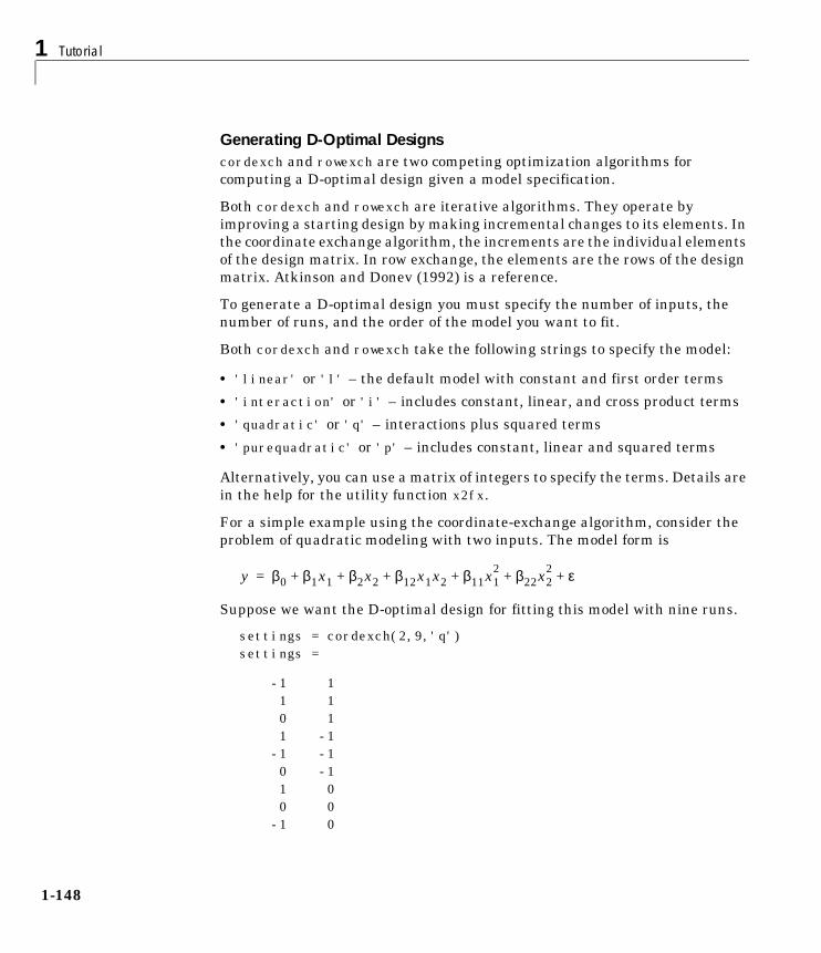
1 Tutorial
1-148
Generating D-Optimal Designscordexch and rowexch are two competing optimization algorithms forcomputing a D-optimal design given a model specification.
Both cordexch and rowexch are iterative algorithms. They operate byimproving a starting design by making incremental changes to its elements. Inthe coordinate exchange algorithm, the increments are the individual elementsof the design matrix. In row exchange, the elements are the rows of the designmatrix. Atkinson and Donev (1992) is a reference.
To generate a D-optimal design you must specify the number of inputs, thenumber of runs, and the order of the model you want to fit.
Both cordexch and rowexch take the following strings to specify the model:
• 'linear' or 'l' – the default model with constant and first order terms
• 'interaction' or 'i' – includes constant, linear, and cross product terms
• 'quadratic' or 'q' – interactions plus squared terms
• 'purequadratic' or 'p' – includes constant, linear and squared terms
Alternatively, you can use a matrix of integers to specify the terms. Details arein the help for the utility function x2fx.
For a simple example using the coordinate-exchange algorithm, consider theproblem of quadratic modeling with two inputs. The model form is
Suppose we want the D-optimal design for fitting this model with nine runs.
settings = cordexch(2,9,'q')settings =
-1 1 1 1 0 1 1 -1 -1 -1 0 -1 1 0 0 0 -1 0
y β0 β1x1 β2x2 β12x1x2 β11x12 β22x2
2 ε+ + + + + +=

Design of Experiments (DOE)
1-149
We can plot the columns of settings against each other to get a better pictureof the design.
h = plot(settings(:,1),settings(:,2),'.');set(gca,'Xtick',[-1 0 1])set(gca,'Ytick',[-1 0 1])set(h,'Markersize',20)
For a simple example using the row-exchange algorithm, consider theinteraction model with two inputs. The model form is
Suppose we want the D-optimal design for fitting this model with four runs.
[settings, X] = rowexch(2,4,'i')
settings =
-1 1 -1 -1 1 -1 1 1
X = 1 -1 1 -1 1 -1 -1 1 1 1 -1 -1 1 1 1 1
The settings matrix shows how to vary the inputs from run to run. The X matrixis the design matrix for fitting the above regression model. The first column of X
-1 0 1-1
0
1
y β0 β1x1 β2x2 β12x1x2 ε+ + + +=

1 Tutorial
1-150
is for fitting the constant term. The last column is the element-wise product ofthe second and third columns.
The associated plot is simple but elegant.
h = plot(settings(:,1),settings(:,2),'.');set(gca,'Xtick',[-1 0 1])set(gca,'Ytick',[-1 0 1])set(h,'Markersize',20)
Augmenting D-Optimal DesignsIn practice, experimentation is an iterative process. We often want to add runsto a completed experiment to learn more about our system. The functiondaugment allows you choose these extra runs optimally.
Suppose we have executed the eight-run design below for fitting a linear modelto four input variables.
settings = cordexch(4,8)settings =
1 -1 1 1 -1 -1 1 -1 -1 1 1 1 1 1 1 -1 -1 1 -1 1 1 -1 -1 1 -1 -1 -1 -1 1 1 -1 -1
-1 0 1-1
0
1

Design of Experiments (DOE)
1-151
This design is adequate to fit the linear model for four inputs, but cannot fit thesix cross-product (interaction) terms. Suppose we are willing to do eight moreruns to fit these extra terms. Here’s how.
[augmented, X] = daugment(settings,8,'i');
augmentedaugmented =
1 -1 1 1 -1 -1 1 -1 -1 1 1 1 1 1 1 -1 -1 1 -1 1 1 -1 -1 1 -1 -1 -1 -1 1 1 -1 -1 -1 -1 -1 1 1 1 1 1 -1 -1 1 1 -1 1 1 -1 1 -1 1 -1 1 -1 -1 -1 -1 1 -1 -1 1 1 -1 1
info = X'*Xinfo =
16 0 0 0 0 0 0 0 0 0 0 0 16 0 0 0 0 0 0 0 0 0 0 0 16 0 0 0 0 0 0 0 0 0 0 0 16 0 0 0 0 0 0 0 0 0 0 0 16 0 0 0 0 0 0 0 0 0 0 0 16 0 0 0 0 0 0 0 0 0 0 0 16 0 0 0 0 0 0 0 0 0 0 0 16 0 0 0 0 0 0 0 0 0 0 0 16 0 0 0 0 0 0 0 0 0 0 0 16 0 0 0 0 0 0 0 0 0 0 0 16
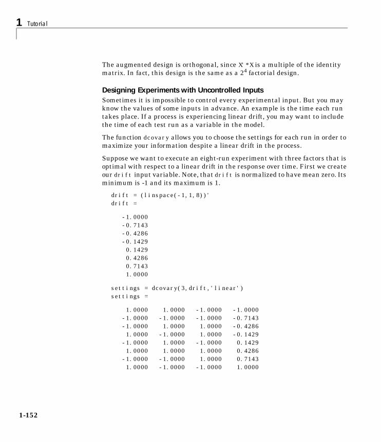
1 Tutorial
1-152
The augmented design is orthogonal, since X'*X is a multiple of the identitymatrix. In fact, this design is the same as a 24 factorial design.
Designing Experiments with Uncontrolled InputsSometimes it is impossible to control every experimental input. But you mayknow the values of some inputs in advance. An example is the time each runtakes place. If a process is experiencing linear drift, you may want to includethe time of each test run as a variable in the model.
The function dcovary allows you to choose the settings for each run in order tomaximize your information despite a linear drift in the process.
Suppose we want to execute an eight-run experiment with three factors that isoptimal with respect to a linear drift in the response over time. First we createour drift input variable. Note, that drift is normalized to have mean zero. Itsminimum is -1 and its maximum is 1.
drift = (linspace(-1,1,8))'drift =
-1.0000 -0.7143 -0.4286 -0.1429 0.1429 0.4286 0.7143 1.0000
settings = dcovary(3,drift,'linear')settings =
1.0000 1.0000 -1.0000 -1.0000 -1.0000 -1.0000 -1.0000 -0.7143 -1.0000 1.0000 1.0000 -0.4286 1.0000 -1.0000 1.0000 -0.1429 -1.0000 1.0000 -1.0000 0.1429 1.0000 1.0000 1.0000 0.4286 -1.0000 -1.0000 1.0000 0.7143 1.0000 -1.0000 -1.0000 1.0000

Demos
1-153
DemosThe Statistics Toolbox has demonstration programs that create an interactiveenvironment for exploring the probability distributions, random numbergeneration, curve fitting, and design of experiments functions. Most of themprovide a graphical user interface that can be used with your real data, not justwith the sample data provided.
The available demos are listed below.
Most of these functions are described below. The nlintool, rstool, andstepwise demos are discussed in earlier sections:
• nlintool: “An Interactive GUI for Nonlinear Fitting and Prediction” onpage 1-104
• rstool: “Exploring Graphs of Multidimensional Polynomials” on page 1-86
• stepwise: “Example: Stepwise Regression” on page 1-88
Demo Purpose
aoctool Interactive graphic prediction of anocova fits
disttool Graphic interaction with probability distributions
glmdemo Generalized linear models slide show
nlintool Interactive fitting of nonlinear models
polytool Interactive graphic prediction of polynomial fits
randtool Interactive control of random number generation
robustdemo Interactive comparison of robust and least squares fits
rsmdemo Design of experiments and regression modeling
rstool Exploring graphs of multidimensional polynomials
stepwise Interactive stepwise regression

1 Tutorial
1-154
The disttool Demo disttool is a graphic environment for developing an intuitive understandingof probability distributions.
The disttool demo has the following features:
• A graph of the cdf (pdf) for the given parameters of a distribution.
• A pop-up menu for changing the distribution function.
• A pop-up menu for changing the function type (cdf <–> pdf).
• Sliders to change the parameter settings.
• Data entry boxes to choose specific parameter values.
• Data entry boxes to change the limits of the parameter sliders.
• Draggable horizontal and vertical reference lines to do interactive evaluationof the function at varying values.
• A data entry box to evaluate the function at a specific x-value.
• For cdf plots, a data entry box on the probability axis (y-axis) to find criticalvalues corresponding to a specific probability.
• A Close button to end the demonstration.

Demos
1-155
Function type pop-up
cdf function
Draggable vertical reference line
Parameter value
Distributions pop-up
cdf value
x value
Parameter control
Draggable horizontal reference line
Upper and lower parameter bounds

1 Tutorial
1-156
The polytool DemoThe polytool demo is an interactive graphic environment for polynomial curvefitting and prediction.
The polytool demo has the following features:
• A graph of the data, the fitted polynomial, and global confidence bounds ona new predicted value.
• y-axis text to display the predicted y-value and its uncertainty at the currentx-value.
• A data entry box to change the degree of the polynomial fit.
• A data entry box to evaluate the polynomial at a specific x-value.
• A draggable vertical reference line to do interactive evaluation of thepolynomial at varying x-values.
• Bounds and Method menus to control the confidence bounds and choosebetween least squares or robust fitting.
• A Close button to end the demonstration.
• An Export list box to store fit results into variables.
You can use polytool to do curve fitting and prediction for any set of x-y data,but, for the sake of demonstration, the Statistics Toolbox provides a data set(polydata.mat) to teach some basic concepts.
To start the demonstration, you must first load the data set.
load polydatawho
Your variables are:
x x1 y y1
The variables x and y are observations made with error from a cubicpolynomial. The variables x1 and y1 are data points from the “true” functionwithout error.
If you do not specify the degree of the polynomial, polytool does a linear fit tothe data.
polytool(x,y)

Demos
1-157
The linear fit is not very good. The bulk of the data with x-values between zeroand two has a steeper slope than the fitted line. The two points to the right aredragging down the estimate of the slope.
In the Degree box at the top, type 3 for a cubic model. Then, drag the verticalreference line to the x-value of 2 (or type 2 in the X Values text box).
Predicted value
Polynomial degree
95% confidence interval
Draggable reference line
Lower confidence bound
Fitted line
Upper confidence bound
x-value
Data point

1 Tutorial
1-158
This graph shows a much better fit to the data. The confidence bounds arecloser together indicating that there is less uncertainty in prediction. The dataat both ends of the plot tracks the fitted curve.
The following sections explore additional aspects of the tool:
• “Confidence Bounds”
• “Overfitting”
Confidence BoundsBy default, the confidence bounds are nonsimultaneous bounds for a newobservation. What does this mean? Let p(x) be the true but unknown functionwe want to estimate. The graph contains the following three curves:
• f(x), our fitted function
• l(x), the lower confidence bounds
• u(x), the upper confidence bounds

Demos
1-159
Suppose we plan to take a new observation at the value . Call it. This new observation has its own error , so it satisfies the
equation
What are the likely values for this new observation? The confidence boundsprovide the answer. The interval [ , ] is a 95% confidence bound for
.
These are the default bounds, but the Bounds menu on the polytool figurewindow provides options for changing the meaning of these bounds. This menuhas options that let you specify whether the bounds are to apply to theestimated function or to a new observation, and whether the bounds should besimultaneous or not. Using these options you can produce any of the followingtypes of confidence bounds.
OverfittingIf the cubic polynomial is a good fit, it is tempting to try a higher orderpolynomial to see if even more precise predictions are possible.
Since the true function is cubic, this amounts to overfitting the data. Use thedata entry box for degree and type 5 for a quintic model.
Simultaneous? For Quantity Yields Confidence Bounds for
Nonsimultaneous Observation
Nonsimultaneous Curve
Simultaneous Observation , globally for any x
Simultaneous Curve , simultaneously for all x
xn 1+yn 1+ xn 1+( ) εn 1+
yn 1+ xn 1+( ) p xn 1+( ) εn 1++=
ln 1+ un 1+yn 1+ xn 1+( )
yn 1+ xn 1+( )
p xn 1+( )
yn 1+ x( )
p x( )

1 Tutorial
1-160
As measured by the confidence bounds, the fit is precise near the data points.But, in the region between the data groups, the uncertainty of prediction risesdramatically.
This bulge in the confidence bounds happens because the data really does notcontain enough information to estimate the higher order polynomial termsprecisely, so even interpolation using polynomials can be risky in some cases.

Demos
1-161
The aoctool DemoThe aoctool demo is an interactive graphical environment for fitting andprediction with analysis of covariance (anocova) models. It is similar to thepolytool demo.
Analysis of covariance is a technique for analyzing grouped data having aresponse (y, the variable to be predicted) and a predictor (x, the variable usedto do the prediction). Using analysis of covariance, you can model y as a linearfunction of x, with the coefficients of the line possibly varying from group togroup. The aoctool function fits the following models for the ith group:
In the fourth model, for example, the intercept varies from one group to thenext, but the slope is the same for each group. In the first model, there is acommon intercept and no slope. In order to make the group coefficients welldetermined, we impose the constraints Σαi = Σβi = 0.
The aoctool demo displays the results of the fit in three figure windows. Onewindow displays estimates of the coefficients (α, αi, β, βi). A second displays ananalysis of variance table that you can use to test whether a more complexmodel is significantly better than a simpler one. The third, main graphicswindow has the following features:
• A graph of the data with superimposed fitted lines and optional confidencebounds.
• y-axis text to display the predicted y-value and its uncertainty at the currentx-value for the current group, if a group is currently selected.
• A data entry box to evaluate the fit at a specific x-value.
• A list box to evaluate the fit for a specific group or to display fitted lines forall groups.
• A draggable vertical reference line to do interactive evaluation of the fit atvarying x-values.
1 same mean
2 separate means
3 same line
4 parallel lines
5 separate lines
y α ε+=
y α αi+( ) ε+=
y α βx ε+ +=
y α αi+( ) βx ε+ +=
y α αi+( ) β βi+( )x ε+ +=

1 Tutorial
1-162
• A Close button to end the demonstration.
• An Export list box to store fit results into variables.
The following section provides an illustrative example.
Example: aoctool with Sample DataThe Statistics Toolbox has a small data set named carsmall with informationabout cars. It is a good sample data set to use with aoctool. You can also useaoctool with your own data.
To start the demonstration, load the data set.
load carsmallwho
Your variables are:
Acceleration Horsepower Model_Year Cylinders MPG Origin Displacement Model Weight
Suppose we want to study the relationship between the weight of a car and itsmileage, and whether this relationship has changed over the years.
Next, start up the tool.
[h,atab,ctab,stats] = aoctool(Weight,MPG,Model_Year);Note: 6 observations with missing values have been removed.
The graphical output consists of the following main window, plus a table ofcoefficient estimates and an analysis of variance table.

Demos
1-163
The group of each data point is coded by its color and symbol, and the fit foreach group has the same color as the data points.
The initial fit models the y variable, MPG, as a linear function of the x variable,Weight. Each group has a separate line. The coefficients of the three lines
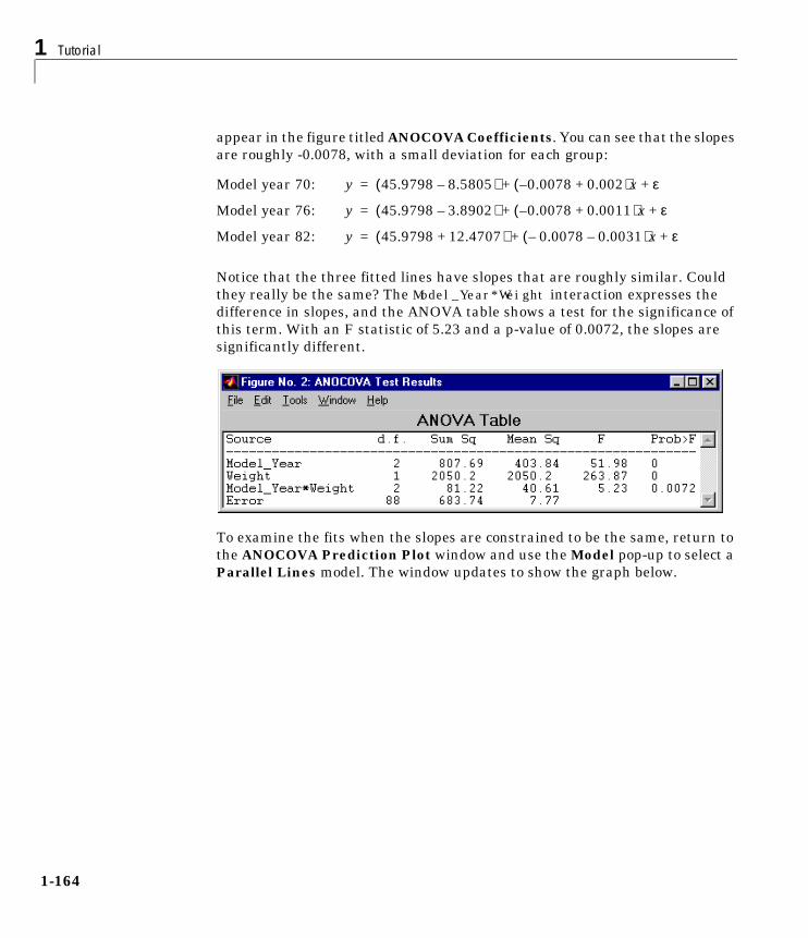
1 Tutorial
1-164
appear in the figure titled ANOCOVA Coefficients. You can see that the slopesare roughly -0.0078, with a small deviation for each group:
Notice that the three fitted lines have slopes that are roughly similar. Couldthey really be the same? The Model_Year*Weight interaction expresses thedifference in slopes, and the ANOVA table shows a test for the significance ofthis term. With an F statistic of 5.23 and a p-value of 0.0072, the slopes aresignificantly different.
To examine the fits when the slopes are constrained to be the same, return tothe ANOCOVA Prediction Plot window and use the Model pop-up to select aParallel Lines model. The window updates to show the graph below.
Model year 70:
Model year 76:
Model year 82:
y 45.9798 8.5805–( ) 0.0078 0.002+–( )x ε+ +=
y 45.9798 3.8902–( ) 0.0078 0.0011+–( )x ε+ +=
y 45.9798 12.4707+( ) 0.0078– 0.0031–( )x ε+ +=

Demos
1-165
Though this fit looks reasonable, we know it is significantly worse than theSeparate Lines model. Use the Model pop-up again to return to the originalmodel.
The following sections focus on two other interesting aspects of aoctool:
• “Confidence Bounds”
• “Multiple Comparisons”
Confidence Bounds. Now we have estimates of the relationship between MPG andWeight for each Model_Year, but how accurate are they? We can superimposeconfidence bounds on the fits by examining them one group at a time. In theModel_Year menu at the lower right of the figure, change the setting fromAll Groups to 82. The data and fits for the other groups are dimmed, andconfidence bounds appear around the 82 fit.

1 Tutorial
1-166
The dashed lines form an envelope around the fitted line for model year 82.Under the assumption that the true relationship is linear, these boundsprovide a 95% confidence region for the true line. Note that the fits for the othermodel years are well outside these confidence bounds for Weight valuesbetween 2000 and 3000.
Sometimes it is more valuable to be able to predict the response value for a newobservation, not just estimate the average response value. Like the polytoolfunction, the aoctool function has a Bounds menu to change the definition ofthe confidence bounds. Use that menu to change from Line to Observation.The resulting wider intervals reflect the uncertainty in the parameterestimates as well as the randomness of a new observation.
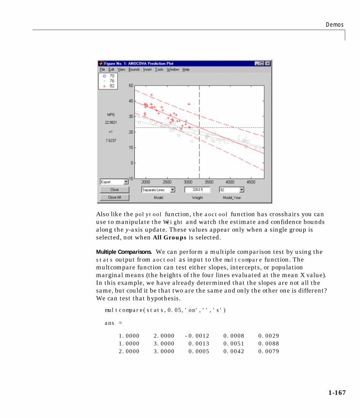
Demos
1-167
Also like the polytool function, the aoctool function has crosshairs you canuse to manipulate the Weight and watch the estimate and confidence boundsalong the y-axis update. These values appear only when a single group isselected, not when All Groups is selected.
Multiple Comparisons. We can perform a multiple comparison test by using thestats output from aoctool as input to the multcompare function. Themultcompare function can test either slopes, intercepts, or populationmarginal means (the heights of the four lines evaluated at the mean X value).In this example, we have already determined that the slopes are not all thesame, but could it be that two are the same and only the other one is different?We can test that hypothesis.
multcompare(stats,0.05,'on','','s')
ans =
1.0000 2.0000 -0.0012 0.0008 0.0029 1.0000 3.0000 0.0013 0.0051 0.0088 2.0000 3.0000 0.0005 0.0042 0.0079

1 Tutorial
1-168
This matrix shows that the estimated difference between the intercepts ofgroups 1 and 2 (1970 and 1976) is 0.0008, and a confidence interval for thedifference is [-0.0012, 0.0029]. There is no significant difference between thetwo. There are significant differences, however, between the intercept for 1982and each of the other two. The graph shows the same information.
Note that the stats structure was created in the initial call to the aoctoolfunction, so it is based on the initial model fit (typically a separate-lines model).If you change the model interactively and want to base your multiplecomparisons on the new model, you need to run aoctool again to get anotherstats structure, this time specifying your new model as the initial model.

Demos
1-169
The randtool Demorandtool is a graphic environment for generating random samples fromvarious probability distributions and displaying the sample histogram.
The randtool demo has the following features:
• A histogram of the sample.
• A pop-up menu for changing the distribution function.
• Sliders to change the parameter settings.
• A data entry box to choose the sample size.
• Data entry boxes to choose specific parameter values.
• Data entry boxes to change the limits of the parameter sliders.
• An Output button to output the current sample to the variable ans.
• A Resample button to allow repetitive sampling with constant sample sizeand fixed parameters.
• A Close button to end the demonstration.
Parameter value
Draw again from the same distribution
Parameter control
Histogram
Upper and lower parameter bounds
Sample size
Distributions pop-up
Output to variable ans

1 Tutorial
1-170
The rsmdemo Demo The rsmdemo utility is an interactive graphic environment that demonstratesthe design of experiments and surface fitting through the simulation of achemical reaction. The goal of the demo is to find the levels of the reactantsneeded to maximize the reaction rate.
There are two parts to the demo:
• “Part 1” – Compare data gathered through trial and error with data from adesigned experiment.
• “Part 2” – Compare response surface (polynomial) modeling with nonlinearmodeling.
Part 1Begin the demo by using the sliders in the Reaction Simulator window tocontrol the partial pressures of three reactants: Hydrogen, n-Pentane, andIsopentane. Each time you click the Run button, the levels for the reactantsand results of the run are entered in the Trial and Error Data window.
Based on the results of previous runs, you can change the levels of thereactants to increase the reaction rate. (The results are determined using anunderlying model that takes into account the noise in the process, so even if youkeep all of the levels the same, the results will vary from run to run.) You areallotted a budget of 13 runs. When you have completed the runs, you can usethe Plot menu on the Trial and Error Data window to plot the relationshipsbetween the reactants and the reaction rate, or click the Analyze button. Whenyou click Analyze, rsmdemo calls the rstool function, which you can then useto try to optimize the results.)
Next, perform another set of 13 runs, this time from a designed experiment. Inthe Experimental Design Data window, click the Do Experiment button.rsmdemo calls the cordexch function to generate a D-optimal design, and then,for each run, computes the reaction rate.
Now use the Plot menu on the Experimental Design Data window to plot therelationships between the levels of the reactants and the reaction rate, or clickthe Response Surface button to call rstool to find the optimal levels of thereactants.

Demos
1-171
Compare the analysis results for the two sets of data. It is likely (though notcertain) that you’ll find some or all of these differences:
• You can fit a full quadratic model with the data from the designedexperiment, but the trial and error data may be insufficient for fitting aquadratic model or interactions model.
• Using the data from the designed experiment, you are more likely to be ableto find levels for the reactants that result in the maximum reaction rate.Even if you find the best settings using the trial and error data, theconfidence bounds are likely to be wider than those from the designedexperiment.
Part 2Now analyze the experimental design data with a polynomial model and anonlinear model, and comparing the results. The true model for the process,which is used to generate the data, is actually a nonlinear model. However,within the range of the data, a quadratic model approximates the true modelquite well.
To see the polynomial model, click the Response Surface button on theExperimental Design Data window. rsmdemo calls rstool, which fits a fullquadratic model to the data. Drag the reference lines to change the levels of thereactants, and find the optimal reaction rate. Observe the width of theconfidence intervals.
Now click the Nonlinear Model button on the Experimental Design Datawindow. rsmdemo calls nlintool, which fits a Hougen-Watson model to thedata. As with the quadratic model, you can drag the reference lines to changethe reactant levels. Observe the reaction rate and the confidence intervals.
Compare the analysis results for the two models. Even though the true modelis nonlinear, you may find that the polynomial model provides a good fit.Because polynomial models are much easier to fit and work with thannonlinear models, a polynomial model is often preferable even when modelinga nonlinear process. Keep in mind, however, that such models are unlikely tobe reliable for extrapolating outside the range of the data.

1 Tutorial
1-172
The glmdemo DemoThe glmdemo function presents a simple slide show describing generalizedlinear models. It presents examples of what functions and distributions areavailable with generalized linear models. It presents an example wheretraditional linear least squares fitting is not appropriate, and shows how to usethe glmfit function to fit a logistic regression model and the glmval functionto compute predictions from that model.
The robustdemo DemoThe robustdemo function presents a simple comparison of least squares androbust fits for a response and a single predictor. You can use robustdemo withyour own data or with the sample data provided.
To begin using robustdemo with the built-in sample data, simply type thefunction name.
robustdemo
The resulting figure presents a scatter plot with two fitted lines. One line is thefit from an ordinary least squares regression. The other is from a robustregression. Along the bottom of the figure are the equations for the fitted lineand the estimated error standard deviation for each fit.
The effect of any point on the least squares fit depends on the residual andleverage for that point. The residual is simply the vertical distance from thepoint to the line. The leverage is a measure of how far the point is from thecenter of the X data.
The effect of any point on the robust fit also depends on the weight assigned tothe point. Points far from the line get lower weight.
You can use the right mouse button to click on any point and see its leastsquares leverage and robust weight.

Demos
1-173
In this example, the rightmost point has a leverage value of 0.35. It is also farfrom the line, so it exerts a large influence on the least squares fit. It has asmall weight, though, so it is effectively excluded from the robust fit.
Using the left mouse button, you can experiment to see how changes in the dataaffect the two fits. Select any point, and drag it to a new location while holdingthe left button down. When you release the point, both fits update.
Bringing the rightmost point closer to the line makes the two fitted lines nearlyidentical. Now, the point has nearly full weight in the robust fit.

1 Tutorial
1-174

Selected Bibliography
1-175
Selected BibliographyAtkinson, A.C., and A.N. Donev, Optimum Experimental Designs, OxfordScience Publications 1992.
Bates, D. and D. Watts. Nonlinear Regression Analysis and Its Applications,John Wiley and Sons. 1988. pp. 271–272.
Bernoulli, J., Ars Conjectandi, Basiliea: Thurnisius [11.19], 1713
Box, G.E.P., W.G. Hunter, and J.S. Hunter. Statistics for Experimenters. Wiley,New York. 1978.
Chatterjee, S. and A.S. Hadi. Influential Observations, High Leverage Points,and Outliers in Linear Regression. Statistical Science, 1986. pp. 379–416.
Dobson, A. J., An Introduction to Generalized Linear Models, 1990, CRC Press.
Efron, B., and R.J. Tibshirani. An Introduction to the Bootstrap, Chapman andHall, New York. 1993.
Evans, M., N. Hastings, and B. Peacock. Statistical Distributions, SecondEdition. John Wiley and Sons, 1993.
Hald, A., Statistical Theory with Engineering Applications, John Wiley andSons, 1960. p. 647.
Hogg, R.V., and J. Ledolter. Engineering Statistics. MacMillan PublishingCompany, 1987.
Johnson, N., and S. Kotz. Distributions in Statistics: Continuous UnivariateDistributions. John Wiley and Sons, 1970.
MuCullagh, P., and J. A. Nelder, Generalized Linear Models, 2nd edition, 1990,Chapman and Hall.
Moore, J., Total Biochemical Oxygen Demand of Dairy Manures. Ph.D. thesis.University of Minnesota, Department of Agricultural Engineering, 1975.
Poisson, S.D., Recherches sur la Probabilité des Jugements en MatiereCriminelle et en Metière Civile, Précédées des Regles Générales du Calcul desProbabilitiés. Paris: Bachelier, Imprimeur-Libraire pour les Mathematiques,1837.
“Student,” On the Probable Error of the Mean. Biometrika, 6:1908. pp. 1–25.

1 Tutorial
1-176
Weibull, W., A Statistical Theory of the Strength of Materials. IngeniorsVetenskaps Akademiens Handlingar, Royal Swedish Institute for EngineeringResearch. Stockholm, Sweden, No. 153. 1939.

2
Reference

2 Reference
2-2
This chapter contains detailed descriptions of all the Statistics Toolboxfunctions. It is divided into two sections:
• “Function Category List” – a list of functions, grouped by subject area
• “Alphabetical List of Functions” – reference pages in alphabetical order
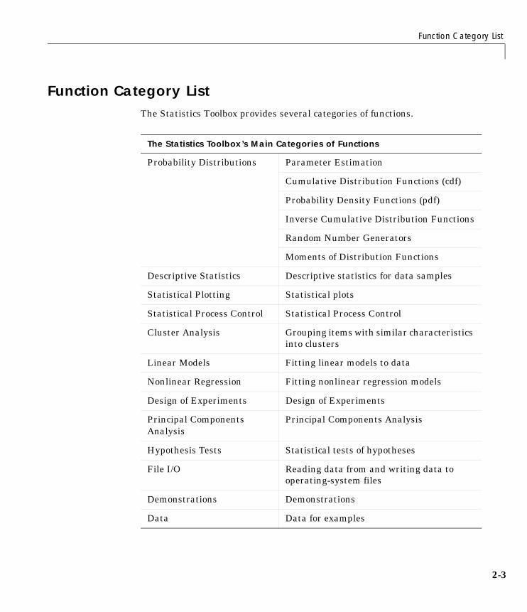
Function Category List
2-3
Function Category ListThe Statistics Toolbox provides several categories of functions.
The Statistics Toolbox’s Main Categories of Functions
Probability Distributions Parameter Estimation
Cumulative Distribution Functions (cdf)
Probability Density Functions (pdf)
Inverse Cumulative Distribution Functions
Random Number Generators
Moments of Distribution Functions
Descriptive Statistics Descriptive statistics for data samples
Statistical Plotting Statistical plots
Statistical Process Control Statistical Process Control
Cluster Analysis Grouping items with similar characteristicsinto clusters
Linear Models Fitting linear models to data
Nonlinear Regression Fitting nonlinear regression models
Design of Experiments Design of Experiments
Principal ComponentsAnalysis
Principal Components Analysis
Hypothesis Tests Statistical tests of hypotheses
File I/O Reading data from and writing data tooperating-system files
Demonstrations Demonstrations
Data Data for examples

2 Reference
2-4
The following tables list the functions in each of these specific areas. The firstseven tables contain probability distribution functions. The remaining tablesdescribe the other categories of functions.
Parameter Estimation
betafit Parameter estimation for the beta distribution
betalike Beta log-likelihood function
binofit Parameter estimation for the binomial distribution
expfit Parameter estimation for the exponential distribution
gamfit Parameter estimation for the gamma distribution
gamlike Gamma log-likelihood function
mle Maximum likelihood estimation
normlike Normal log-likelihood function
normfit Parameter estimation for the normal distribution
poissfit Parameter estimation for the Poisson distribution
unifit Parameter estimation for the uniform distribution
Cumulative Distribution Functions (cdf)
betacdf Beta cdf
binocdf Binomial cdf
cdf Parameterized cdf routine
chi2cdf Chi-square cdf
expcdf Exponential cdf

Function Category List
2-5
fcdf F cdf
gamcdf Gamma cdf
geocdf Geometric cdf
hygecdf Hypergeometric cdf
logncdf Lognormal cdf
nbincdf Negative binomial cdf
ncfcdf Noncentral F cdf
nctcdf Noncentral t cdf
ncx2cdf Noncentral Chi-square cdf
normcdf Normal (Gaussian) cdf
poisscdf Poisson cdf
raylcdf Rayleigh cdf
tcdf Student’s t cdf
unidcdf Discrete uniform cdf
unifcdf Continuous uniform cdf
weibcdf Weibull cdf
Probability Density Functions (pdf)
betapdf Beta pdf
binopdf Binomial pdf
chi2pdf Chi-square pdf
exppdf Exponential pdf
Cumulative Distribution Functions (cdf) (Continued)

2 Reference
2-6
fpdf F pdf
gampdf Gamma pdf
geopdf Geometric pdf
hygepdf Hypergeometric pdf
normpdf Normal (Gaussian) pdf
lognpdf Lognormal pdf
nbinpdf Negative binomial pdf
ncfpdf Noncentral F pdf
nctpdf Noncentral t pdf
ncx2pdf Noncentral Chi-square pdf
pdf Parameterized pdf routine
poisspdf Poisson pdf
raylpdf Rayleigh pdf
tpdf Student’s t pdf
unidpdf Discrete uniform pdf
unifpdf Continuous uniform pdf
weibpdf Weibull pdf
Inverse Cumulative Distribution Functions
betainv Beta critical values
binoinv Binomial critical values
chi2inv Chi-square critical values
Probability Density Functions (pdf) (Continued)
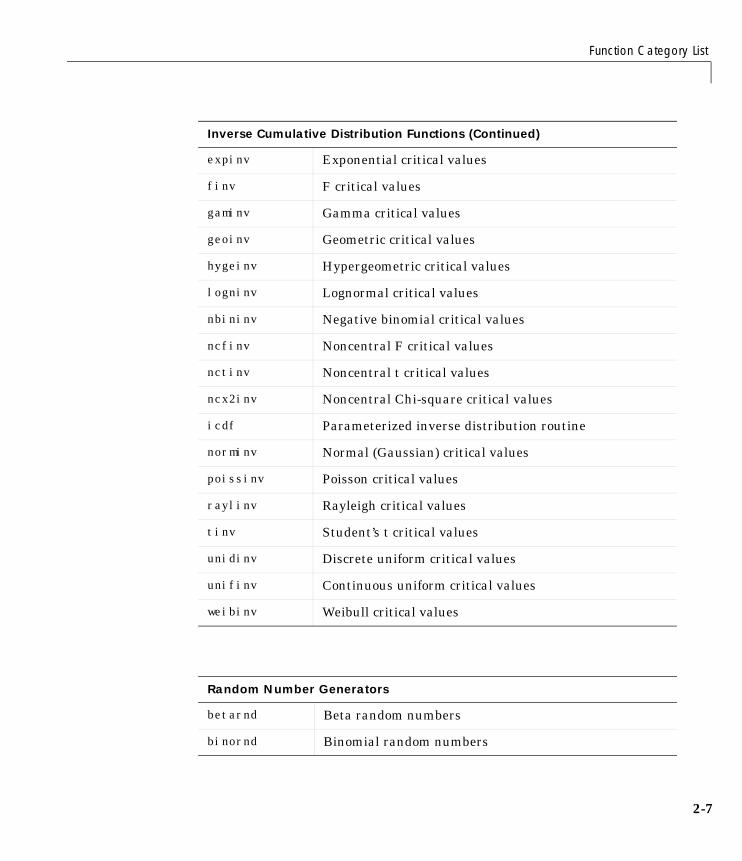
Function Category List
2-7
expinv Exponential critical values
finv F critical values
gaminv Gamma critical values
geoinv Geometric critical values
hygeinv Hypergeometric critical values
logninv Lognormal critical values
nbininv Negative binomial critical values
ncfinv Noncentral F critical values
nctinv Noncentral t critical values
ncx2inv Noncentral Chi-square critical values
icdf Parameterized inverse distribution routine
norminv Normal (Gaussian) critical values
poissinv Poisson critical values
raylinv Rayleigh critical values
tinv Student’s t critical values
unidinv Discrete uniform critical values
unifinv Continuous uniform critical values
weibinv Weibull critical values
Random Number Generators
betarnd Beta random numbers
binornd Binomial random numbers
Inverse Cumulative Distribution Functions (Continued)

2 Reference
2-8
chi2rnd Chi-square random numbers
exprnd Exponential random numbers
frnd F random numbers
gamrnd Gamma random numbers
geornd Geometric random numbers
hygernd Hypergeometric random numbers
lognrnd Lognormal random numbers
nbinrnd Negative binomial random numbers
ncfrnd Noncentral F random numbers
nctrnd Noncentral t random numbers
ncx2rnd Noncentral Chi-square random numbers
normrnd Normal (Gaussian) random numbers
poissrnd Poisson random numbers
raylrnd Rayleigh random numbers
random Parameterized random number routine
trnd Student’s t random numbers
unidrnd Discrete uniform random numbers
unifrnd Continuous uniform random numbers
weibrnd Weibull random numbers
Random Number Generators (Continued)

Function Category List
2-9
Moments of Distribution Functions
betastat Beta mean and variance
binostat Binomial mean and variance
chi2stat Chi-square mean and variance
expstat Exponential mean and variance
fstat F mean and variance
gamstat Gamma mean and variance
geostat Geometric mean and variance
hygestat Hypergeometric mean and variance
lognstat Lognormal mean and variance
nbinstat Negative binomial mean and variance
ncfstat Noncentral F mean and variance
nctstat Noncentral t mean and variance
ncx2stat Noncentral Chi-square mean and variance
normstat Normal (Gaussian) mean and variance
poisstat Poisson mean and variance
raylstat Rayleigh mean and variance
tstat Student’s t mean and variance
unidstat Discrete uniform mean and variance
unifstat Continuous uniform mean and variance
weibstat Weibull mean and variance

2 Reference
2-10
Descriptive Statistics
corrcoef Correlation coefficients (in MATLAB)
cov Covariance matrix (in MATLAB)
geomean Geometric mean
harmmean Harmonic mean
iqr Interquartile range
kurtosis Sample kurtosis
mad Mean absolute deviation
mean Arithmetic average (in MATLAB)
median 50th percentile (in MATLAB)
moment Central moments of all orders
nanmax Maximum ignoring missing data
nanmean Average ignoring missing data
nanmedian Median ignoring missing data
nanmin Minimum ignoring missing data
nanstd Standard deviation ignoring missing data
nansum Sum ignoring missing data
prctile Empirical percentiles of a sample
range Sample range
skewness Sample skewness
std Standard deviation (in MATLAB)
trimmean Trimmed mean
var Variance

Function Category List
2-11
Statistical Plotting
boxplot Box plots
errorbar Error bar plot
fsurfht Interactive contour plot of a function
gline Interactive line drawing
gname Interactive point labeling
lsline Add least-squares fit line to plotted data
normplot Normal probability plots
pareto Pareto charts
qqplot Quantile-Quantile plots
rcoplot Regression case order plot
refcurve Reference polynomial
refline Reference line
surfht Interactive interpolating contour plot
weibplot Weibull plotting
Statistical Process Control
capable Quality capability indices
capaplot Plot of process capability
ewmaplot Exponentially weighted moving average plot
histfit Histogram and normal density curve
normspec Plot normal density between limits

2 Reference
2-12
schart Time plot of standard deviation
xbarplot Time plot of means
Cluster Analysis
cluster Create clusters from linkage output
clusterdata Create clusters from a dataset
cophenet Calculate the cophenetic correlation coefficient
dendrogram Plot a hierarchical tree in a dendrogram graph
inconsistent Calculate the inconsistency values of objects in a clusterhierarchy tree
linkage Link objects in a dataset into a hierarchical tree ofbinary clusters
pdist Calculate the pairwise distance between objects in adataset
squareform Reformat output of pdist function from vector to squarematrix
zscore Normalize a dataset before calculating the distance
Linear Models
anova1 One-way Analysis of Variance (ANOVA)
anova2 Two-way Analysis of Variance
lscov Regression given a covariance matrix (in MATLAB)
Statistical Process Control (Continued)

Function Category List
2-13
polyconf Polynomial prediction with confidence intervals
polyfit Polynomial fitting (in MATLAB)
polyval Polynomial prediction (in MATLAB)
regress Multiple linear regression
ridge Ridge regression
rstool Response surface tool
stepwise Stepwise regression GUI
Nonlinear Regression
nlinfit Nonlinear least-squares fitting
nlintool Prediction graph for nonlinear fits
nlparci Confidence intervals on parameters
nlpredci Confidence intervals for prediction
nnls Nonnegative least squares (in MATLAB)
Design of Experiments
cordexch D-optimal design using coordinate exchange
daugment D-optimal augmentation of designs
dcovary D-optimal design with fixed covariates
ff2n Two-level full factorial designs
fullfact Mixed level full factorial designs
Linear Models (Continued)
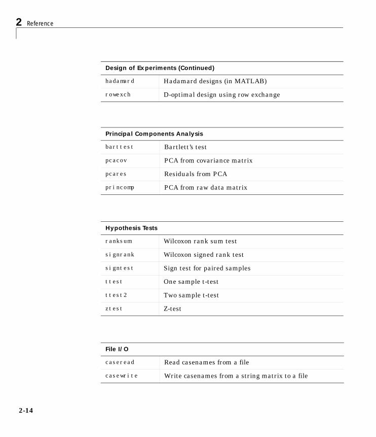
2 Reference
2-14
hadamard Hadamard designs (in MATLAB)
rowexch D-optimal design using row exchange
Principal Components Analysis
barttest Bartlett’s test
pcacov PCA from covariance matrix
pcares Residuals from PCA
princomp PCA from raw data matrix
Hypothesis Tests
ranksum Wilcoxon rank sum test
signrank Wilcoxon signed rank test
signtest Sign test for paired samples
ttest One sample t-test
ttest2 Two sample t-test
ztest Z-test
File I/O
caseread Read casenames from a file
casewrite Write casenames from a string matrix to a file
Design of Experiments (Continued)
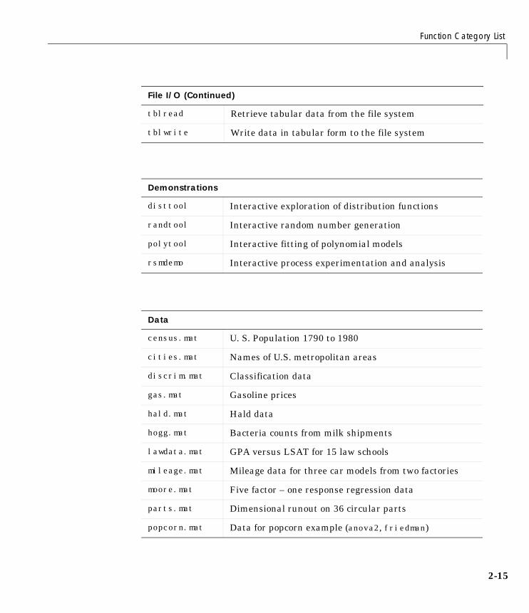
Function Category List
2-15
tblread Retrieve tabular data from the file system
tblwrite Write data in tabular form to the file system
Demonstrations
disttool Interactive exploration of distribution functions
randtool Interactive random number generation
polytool Interactive fitting of polynomial models
rsmdemo Interactive process experimentation and analysis
Data
census.mat U. S. Population 1790 to 1980
cities.mat Names of U.S. metropolitan areas
discrim.mat Classification data
gas.mat Gasoline prices
hald.mat Hald data
hogg.mat Bacteria counts from milk shipments
lawdata.mat GPA versus LSAT for 15 law schools
mileage.mat Mileage data for three car models from two factories
moore.mat Five factor – one response regression data
parts.mat Dimensional runout on 36 circular parts
popcorn.mat Data for popcorn example (anova2, friedman)
File I/O (Continued)

2 Reference
2-16
polydata.mat Data for polytool demo
reaction.mat Reaction kinetics data
sat.dat ASCII data for tblread example
Data (Continued)

anova1
2-17
2anova1
2
Purpose One-way Analysis of Variance (ANOVA).
Syntax p = anova1(X)p = anova1(X,group)p = anova1(X,group,'displayopt')[p,table] = anova1(...)[p,table,stats] = anova1(...)
Description p = anova1(X) performs a balanced one-way ANOVA for comparing themeans of two or more columns of data in the m-by-n matrix X, where eachcolumn represents an independent sample containing m mutually independentobservations. The function returns the p-value for the null hypothesis that allsamples in X are drawn from the same population (or from differentpopulations with the same mean).
If the p-value is near zero, this casts doubt on the null hypothesis and suggeststhat at least one sample mean is significantly different than the other samplemeans. The choice of a critical p-value to determine whether the result isjudged “statistically significant” is left to the researcher. It is common todeclare a result significant if the p-value is less than 0.05 or 0.01.
The anova1 function displays two figures. The first figure is the standardANOVA table, which divides the variability of the data in X into two parts:
• Variability due to the differences among the column means (variabilitybetween groups)
• Variability due to the differences between the data in each column and thecolumn mean (variability within groups)
The ANOVA table has six columns:
• The first shows the source of the variability.
• The second shows the Sum of Squares (SS) due to each source.
• The third shows the degrees of freedom (df) associated with each source.
• The fourth shows the Mean Squares (MS) for each source, which is the ratioSS/df.
• The fifth shows the F statistic, which is the ratio of the MS’s.
• The sixth shows the p-value, which is derived from the cdf of F. As Fincreases, the p-value decreases.

anova1
2-18
The second figure displays box plots of each column of X. Large differences inthe center lines of the box plots correspond to large values of F andcorrespondingly small p-values.
p = anova1(X,group) uses the values in group (a character array or cellarray) as labels for the box plot of the samples in X, when X is a matrix. Eachrow of group contains the label for the data in the corresponding column of X,so group must have length equal to the number of columns in X.
When X is a vector, anova1 performs a one-way ANOVA on the samplescontained in X, as indexed by input group (a vector, character array, or cellarray). Each element in group identifies the group (i.e., sample) to which thecorresponding element in vector X belongs, so group must have the same lengthas X. The labels contained in group are also used to annotate the box plot. Thevector-input form of anova1 does not require equal numbers of observations ineach sample, so it is appropriate for unbalanced data.
It is not necessary to label samples sequentially (1, 2, 3, ...). For example, if Xcontains measurements taken at three different temperatures, -27°, 65°, and110°, you could use these numbers as the sample labels in group. If a row ofgroup contains an empty cell or empty string, that row and the correspondingobservation in X are disregarded. NaNs in either input are similarly ignored.
p = anova1(X,group,'displayopt') enables the ANOVA table and box plotdisplays when 'displayopt' is 'on' (default) and suppresses the displayswhen 'displayopt' is 'off'.
[p,table] = anova1(...) returns the ANOVA table (including column androw labels) in cell array table. (You can copy a text version of the ANOVA tableto the clipboard by using the Copy Text item on the Edit menu.)
[p,table,stats] = anova1(...) returns a stats structure that you can useto perform a follow-up multiple comparison test. The anova1 test evaluates thehypothesis that the samples all have the same mean against the alternativethat the means are not all the same. Sometimes it is preferable to perform atest to determine which pairs of means are significantly different, and whichare not. You can use the multcompare function to perform such tests bysupplying the stats structure as input.

anova1
2-19
AssumptionsThe ANOVA test makes the following assumptions about the data in X:
• All sample populations are normally distributed.
• All sample populations have equal variance.
• All observations are mutually independent.
The ANOVA test is known to be robust to modest violations of the first twoassumptions.
Examples Example 1The five columns of X are the constants one through five plus a random normaldisturbance with mean zero and standard deviation one.
X = meshgrid(1:5)
X =
1 2 3 4 5 1 2 3 4 5 1 2 3 4 5 1 2 3 4 5 1 2 3 4 5
X = X + normrnd(0,1,5,5)
X =
2.1650 3.6961 1.5538 3.6400 4.9551 1.6268 2.0591 2.2988 3.8644 4.2011 1.0751 3.7971 4.2460 2.6507 4.2348 1.3516 2.2641 2.3610 2.7296 5.8617 0.3035 2.8717 3.5774 4.9846 4.9438
p = anova1(X)
p =
5.9952e-005

anova1
2-20
The very small p-value of 6e-5 indicates that differences between the columnmeans are highly significant. The probability of this outcome under the nullhypothesis (i.e., the probability that samples actually drawn from the samepopulation would have means differing by the amounts seen in X) is less than6 in 100,000. The test therefore strongly supports the alternate hypothesis,that one or more of the samples are drawn from populations with differentmeans.
Example 2The following example comes from a study of the material strength ofstructural beams in Hogg (1987). The vector strength measures the deflectionof a beam in thousandths of an inch under 3,000 pounds of force. Strongerbeams deflect less. The civil engineer performing the study wanted todetermine whether the strength of steel beams was equal to the strength of twomore expensive alloys. Steel is coded 'st' in the vector alloy. The othermaterials are coded 'al1' and 'al2'.
1 2 3 4 5
1
2
3
4
5
6
Val
ues
Column Number

anova1
2-21
strength = [82 86 79 83 84 85 86 87 74 82 78 75 76 77 79 ...79 77 78 82 79];
alloy = {'st','st','st','st','st','st','st','st',...'al1','al1','al1','al1','al1','al1',...'al2','al2','al2','al2','al2','al2'};
Though alloy is sorted in this example, you do not need to sort the groupingvariable.
p = anova1(strength,alloy)
p =
1.5264e-004
The p-value indicates that the three alloys are significantly different. The boxplot confirms this graphically and shows that the steel beams deflect more thanthe more expensive alloys.
st al1 al2
74
76
78
80
82
84
86
Val
ues

anova1
2-22
References Hogg, R. V., and J. Ledolter. Engineering Statistics. MacMillan PublishingCompany, 1987.
See Also anova2, anovan, boxplot, ttest
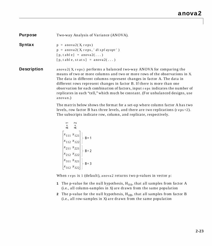
anova2
2-23
2anova2Purpose Two-way Analysis of Variance (ANOVA).
Syntax p = anova2(X,reps) p = anova2(X,reps,'displayopt') [p,table] = anova2(...)[p,table,stats] = anova2(...)
Description anova2(X,reps) performs a balanced two-way ANOVA for comparing themeans of two or more columns and two or more rows of the observations in X.The data in different columns represent changes in factor A. The data indifferent rows represent changes in factor B. If there is more than oneobservation for each combination of factors, input reps indicates the number ofreplicates in each “cell,” which much be constant. (For unbalanced designs, useanovan.)
The matrix below shows the format for a set-up where column factor A has twolevels, row factor B has three levels, and there are two replications (reps=2).The subscripts indicate row, column, and replicate, respectively.
When reps is 1 (default), anova2 returns two p-values in vector p:
1 The p-value for the null hypothesis, H0A, that all samples from factor A(i.e., all column-samples in X) are drawn from the same population
2 The p-value for the null hypothesis, H0B, that all samples from factor B(i.e., all row-samples in X) are drawn from the same population
x111 x121
x112 x122
x211 x221
x212 x222
x311 x321
x312 x322B = 3
B = 2
B = 1
A =
1
A =
2

anova2
2-24
When reps is greater than 1, anova2 returns a third p-value in vector p:
3 The p-value for the null hypothesis, H0AB, that the effects due to factorsA and B are additive (i.e., that there is no interaction between factorsA and B)
If any p-value is near zero, this casts doubt on the associated null hypothesis.A sufficiently small p-value for H0A suggests that at least one column-samplemean is significantly different that the other column-sample means; i.e., thereis a main effect due to factor A. A sufficiently small p-value for H0B suggeststhat at least one row-sample mean is significantly different than the otherrow-sample means; i.e., there is a main effect due to factor B. A sufficientlysmall p-value for H0AB suggests that there is an interaction between factors Aand B. The choice of a limit for the p-value to determine whether a result is“statistically significant” is left to the researcher. It is common to declare aresult significant if the p-value is less than 0.05 or 0.01.
anova2 also displays a figure showing the standard ANOVA table, whichdivides the variability of the data in X into three or four parts depending on thevalue of reps:
• The variability due to the differences among the column means
• The variability due to the differences among the row means
• The variability due to the interaction between rows and columns (if reps isgreater than its default value of one)
• The remaining variability not explained by any systematic source
The ANOVA table has five columns:
• The first shows the source of the variability.
• The second shows the Sum of Squares (SS) due to each source.
• The third shows the degrees of freedom (df) associated with each source.
• The fourth shows the Mean Squares (MS), which is the ratio SS/df.
• The fifth shows the F statistics, which is the ratio of the mean squares.
p = anova2(X,reps,'displayopt') enables the ANOVA table display when'displayopt' is 'on' (default) and suppresses the display when 'displayopt'is 'off'.

anova2
2-25
[p,table] = anova2(...) returns the ANOVA table (including column androw labels) in cell array table. (You can copy a text version of the ANOVA tableto the clipboard by using the Copy Text item on the Edit menu.)
[p,table,stats] = anova2(...) returns a stats structure that you can useto perform a follow-up multiple comparison test.
The anova2 test evaluates the hypothesis that the row, column, and interactioneffects are all the same, against the alternative that they are not all the same.Sometimes it is preferable to perform a test to determine which pairs of effectsare significantly different, and which are not. You can use the multcomparefunction to perform such tests by supplying the stats structure as input.
Examples The data below come from a study of popcorn brands and popper type (Hogg1987). The columns of the matrix popcorn are brands (Gourmet, National, andGeneric). The rows are popper type (Oil and Air.) The study popped a batch ofeach brand three times with each popper. The values are the yield in cups ofpopped popcorn.
load popcorn
popcorn
popcorn =
5.5000 4.5000 3.5000 5.5000 4.5000 4.0000 6.0000 4.0000 3.0000 6.5000 5.0000 4.0000 7.0000 5.5000 5.0000 7.0000 5.0000 4.5000
p = anova2(popcorn,3)
p =
0.0000 0.0001 0.7462

anova2
2-26
The vector p shows the p-values for the three brands of popcorn, 0.0000, thetwo popper types, 0.0001, and the interaction between brand and poppertype, 0.7462. These values indicate that both popcorn brand and popper typeaffect the yield of popcorn, but there is no evidence of a synergistic (interaction)effect of the two.
The conclusion is that you can get the greatest yield using the Gourmet brandand an Air popper (the three values popcorn(4:6,1)).
Reference Hogg, R. V. and J. Ledolter. Engineering Statistics. MacMillan PublishingCompany, 1987.
See Also anova1, anovan
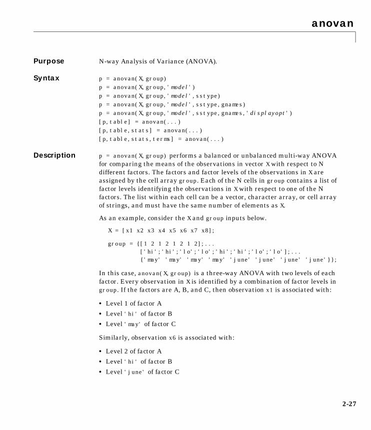
anovan
2-27
2anovanPurpose N-way Analysis of Variance (ANOVA).
Syntax p = anovan(X,group) p = anovan(X,group,'model')p = anovan(X,group,'model',sstype) p = anovan(X,group,'model',sstype,gnames) p = anovan(X,group,'model',sstype,gnames,'displayopt') [p,table] = anovan(...)[p,table,stats] = anovan(...) [p,table,stats,terms] = anovan(...)
Description p = anovan(X,group) performs a balanced or unbalanced multi-way ANOVAfor comparing the means of the observations in vector X with respect to Ndifferent factors. The factors and factor levels of the observations in X areassigned by the cell array group. Each of the N cells in group contains a list offactor levels identifying the observations in X with respect to one of the Nfactors. The list within each cell can be a vector, character array, or cell arrayof strings, and must have the same number of elements as X.
As an example, consider the X and group inputs below.
X = [x1 x2 x3 x4 x5 x6 x7 x8];
group = {[1 2 1 2 1 2 1 2];...['hi';'hi';'lo';'lo';'hi';'hi';'lo';'lo'];...{'may' 'may' 'may' 'may' 'june' 'june' 'june' 'june'}};
In this case, anovan(X,group) is a three-way ANOVA with two levels of eachfactor. Every observation in X is identified by a combination of factor levels ingroup. If the factors are A, B, and C, then observation x1 is associated with:
• Level 1 of factor A
• Level 'hi' of factor B
• Level 'may' of factor C
Similarly, observation x6 is associated with:
• Level 2 of factor A
• Level 'hi' of factor B
• Level 'june' of factor C

anovan
2-28
Output vector p contains p-values for the null hypotheses on the N maineffects. Element p(1) contains the p-value for the null hypotheses, H0A, thatsamples at all levels of factor A are drawn from the same population,element p(2) contains the p-value for the null hypotheses, H0B, that samplesat all levels of factor B are drawn from the same population, and so on.
If any p-value is near zero, this casts doubt on the associated null hypothesis.For example, a sufficiently small p-value for H0A suggests that at least oneA-sample mean is significantly different that the other A-sample means;i.e., there is a main effect due to factor A. The choice of a limit for the p-valueto determine whether a result is “statistically significant” is left to theresearcher. It is common to declare a result significant if the p-value is lessthan 0.05 or 0.01.
anovan also displays a figure showing the standard ANOVA table, which bydefault divides the variability of the data in X into:
• The variability due to differences between the levels of each factor accountedfor in the model (one row for each factor)
• The remaining variability not explained by any systematic source
The ANOVA table has six columns:
• The first shows the source of the variability.
• The second shows the Sum of Squares (SS) due to each source.
• The third shows the degrees of freedom (df) associated with each source.
• The fourth shows the Mean Squares (MS), which is the ratio SS/df.
• The fifth shows the F statistics, which is the ratio of the mean squares.
• The sixth shows the p-values for the F statistics.
p = anovan(X,group,'model') performs the ANOVA using the modelspecified by 'model', where 'model' can be 'linear', 'interaction', 'full',or an integer or vector. The default 'linear'model computes only the p-valuesfor the null hypotheses on the N main effects. The 'interaction' modelcomputes the p-values for null hypotheses on the N main effects and thetwo-factor interactions. The 'full' model computes the p-values for nullhypotheses on the N main effects and interactions at all levels.
N2� �
� �

anovan
2-29
For an integer value of 'model', k (k ≤ N), anovan computes all interactionlevels through the kth level. The values k=1 and k=2 are equivalent to the'linear' and 'interaction' specifications, respectively, while the value k=Nis equivalent to the 'full' specification.
For more precise control over the main and interaction terms that anovancomputes, 'model' can specify a vector containing one element for each mainor interaction term to include in the ANOVA model. Each vector elementencodes the corresponding ANOVA term as the decimal equivalent of an N-bitnumber, where N is the number of factors. The table below illustrates thecoding for a 3-factor ANOVA.
For example, if 'model' is the vector [2 4 6], then output vector p containsthe p-values for the null hypotheses on the main effects B and C and theinteraction effect BC, in that order. A simple way to generate the 'model'vector is to modify the terms output, which codes the terms in the currentmodel using the format described above. If anovan returned [2 4 6] for terms,for example, and there was no significant result for interaction BC, you couldrecompute the ANOVA on just the main effects B and C by specifying [2 4] for'model'.
p = anovan(X,group,'model',sstype) computes the ANOVA using the typeof sum-of-squares specified by sstype, which can be 1, 2, or 3 to designateType 1, Type 2, or Type 3 sum-of-squares, respectively. The default is 3. Thevalue of sstype only influences computations on unbalanced data.
3-bit Code Decimal Value Corresponding ANOVA Terms
[0 0 1] 1 Main term A
[0 1 0] 2 Main term B
[1 0 0] 4 Main term C
[0 1 1] 3 Interaction term AB
[1 1 0] 6 Interaction term BC
[1 0 1] 5 Interaction term AC
[1 1 1] 7 Interaction term ABC

anovan
2-30
The sum of squares for any term is determined by comparing two models. TheType 1 sum of squares for a term is the reduction in residual sum of squaresobtained by adding that term to a fit that already includes the terms listedbefore it. The Type 2 sum of squares is the reduction in residual sum of squaresobtained by adding that term to a model consisting of all other terms that donot contain the term in question. The Type 3 sum of squares is the reduction inresidual sum of squares obtained by adding that term to a model containing allother terms, but with their effects constrained to obey the usual “sigmarestrictions” that make models estimable.
Suppose we are fitting a model with two factors and their interaction, and thatthe terms appear in the order A, B, AB. Let R(·) represent the residual sum ofsquares for a model, so for example R(A,B,AB) is the residual sum of squaresfitting the whole model, R(A) is the residual sum of squares fitting just themain effect of A, and R(1) is the residual sum of squares fitting just the mean.The three types of sums of squares are as follows:
The models for Type 3 sum of squares have sigma restrictions imposed. Thismeans, for example, that in fitting R(B,AB), the array of AB effects isconstrained to sum to 0 over A for each value of B, and over B for each valueof A.
p = anovan(X,group,'model',sstype,gnames) uses the string values incharacter array gnames to label the N experimental factors in the ANOVAtable. The array can be a string matrix with one row per observation, or a cellarray of strings with one element per observation. When gnames is notspecified, the default labels 'X1', 'X2', 'X3', ..., 'XN' are used.
p = anovan(X,group,'model',sstype,gnames,'displayopt') enables theANOVA table display when 'displayopt' is 'on' (default) and suppresses thedisplay when 'displayopt' is 'off'.
Term Type 1 SS Type 2 SS Type 3 SS
A R(1)-R(A) R(B)-R(A,B) R(B,AB)-R(A,B,AB)
B R(A)-R(A,B) R(A)-R(A,B) R(A,AB)-R(A,B,AB)
AB R(A,B)-R(A,B,AB) R(A,B)-R(A,B,AB) R(A,B)-R(A,B,AB)

anovan
2-31
[p,table] = anovan(...) returns the ANOVA table (including factor labels)in cell array table. (You can copy a text version of the ANOVA table to theclipboard by using the Copy Text item on the Edit menu.)
[p,table,stats] = anovan(...) returns a stats structure that you can useto perform a follow-up multiple comparison test.
The anovan test evaluates the hypothesis that the different levels of a factor (ormore generally, a term) have the same effect, against the alternative that theydo not all have the same effect. Sometimes it is preferable to perform a test todetermine which pairs of levels are significantly different, and which are not.You can use the multcompare function to perform such tests by supplying thestats structure as input.
[p,table,stats,terms] = anovan(...) returns the main and interactionterms used in the ANOVA computations. The terms are encoded in outputvector terms using the same format described above for input 'model'. When'model' itself is specified in this vector format, the vector returned in terms isidentical.
Examples In the previous section we used anova2 to analyze the effects of two factors ona response in a balanced design. For a design that is not balanced, we can useanovan instead.
The dataset carbig contains a number of measurements on 406 cars. Let’sstudy how the mileage depends on where and when the cars were made.
load carbiganovan(MPG,{org when},2,3,{'Origin';'Mfg date'})
ans = 0 0 0.30587
The p-value for the interaction term is not small, indicating little evidence thatthe effect of the car’s year or manufacture (when) depends on where the car wasmade (org). The linear effects of those two factors, though, are significant.

anovan
2-32
Reference Hogg, R. V. and J. Ledolter. Engineering Statistics. MacMillan PublishingCompany, 1987.
See Also anova1, anova2, multcompare

aoctool
2-33
2aoctoolPurpose Interactive plot for fitting and predicting analysis of covariance models.
Syntax aoctool(x,y,g)aoctool(x,y,g,alpha)aoctool(x,y,g,alpha,xname,yname,gname)aoctool(x,y,g,alpha,xname,yname,gname,'displayopt')aoctool(x,y,g,alpha,xname,yname,gname,'displayopt','model')h = aoctool(...)[h,atab,ctab] = aoctool(...)[h,atab,ctab,stats] = aoctool(...)
Description aoctool(x,y,g) fits a separate line to the column vectors, x and y, for eachgroup defined by the values in the array g. These types of models are known asone-way analysis of covariance (ANOCOVA) models. The output consists ofthree figures:
• An interactive graph of the data and prediction curves
• An ANOVA table
• A table of parameter estimates
You can use the figures to change models and to test different parts of themodel. More information about interactive use of the aoctool function appearson “The aoctool Demo” on page 1-161.
aoctool(x,y,g,alpha) determines the confidence levels of the predictionintervals. The confidence level is 100*(1-alpha)%. The default value of alphais 0.05.
aoctool(x,y,g,alpha,xname,yname,gname) specifies the name to use for thex, y, and g variables in the graph and tables. If you enter simple variable namesfor the x, y, and g arguments, the aoctool function uses those names. If youenter an expression for one of these arguments, you can specify a name to usein place of that expression by supplying these arguments. For example, if youenter m(:,2) as the x argument, you might choose to enter 'Col 2' as thexname argument.
aoctool(x,y,g,alpha,xname,yname,gname,'displayopt') enables thegraph and table displays when 'displayopt' is 'on' (default) and suppressesthose displays when 'displayopt' is 'off'.

aoctool
2-34
aoctool(x,y,g,alpha,xname,yname,gname,'displayopt','model')specifies the initial model to fit. The value of 'model' can be any of thefollowing:
• 'same mean' – fit a single mean, ignoring grouping
• 'separate means' – fit a separate mean to each group
• 'same line' – fit a single line, ignoring grouping
• 'parallel lines' – fit a separate line to each group, but constrain the linesto be parallel
• 'separate lines' – fit a separate line to each group, with no constraints
h = aoctool(...) returns a vector of handles to the line objects in the plot.
[h,atab,ctab] = aoctool(...) returns cell arrays containing the entries inANOVA table (atab) and the table of coefficient estimates (ctab). (You can copya text version of either table to the clipboard by using the Copy Text item onthe Edit menu.)
[h,atab,ctab,stats] = aoctool(...) returns a stats structure that youcan use to perform a follow-up multiple comparison test. The ANOVA tableoutput includes tests of the hypotheses that the slopes or intercepts are all thesame, against a general alternative that they are not all the same. Sometimesit is preferable to perform a test to determine which pairs of values aresignificantly different, and which are not. You can use the multcomparefunction to perform such tests by supplying the stats structure as input. Youcan test either the slopes, the intercepts, or population marginal means (theheights of the curves at the mean x value).
Example This example illustrates how to fit different models non-interactively. First, weload the smaller car dataset and fit a separate-slopes model, then examine thecoefficient estimates.
[h,a,c,s] = aoctool(Weight,MPG,Model_Year,0.05,...'','','','off','separate lines');
c(:,1:2)

aoctool
2-35
ans = 'Term' 'Estimate' 'Intercept' [45.97983716833132] ' 70' [-8.58050531454973] ' 76' [-3.89017396094922] ' 82' [12.47067927549897] 'Slope' [-0.00780212907455] ' 70' [ 0.00195840368824] ' 76' [ 0.00113831038418] ' 82' [-0.00309671407243]
Roughly speaking, the lines relating MPG to Weight have an intercept close to45.98 and a slope close to -0.0078. Each group’s coefficients are offset fromthese values somewhat. For instance, the intercept for the cars made in 1970is 45.98-8.58 = 37.40.
Next, we try a fit using parallel lines. (If we had examined the ANOVA table,we would have found that the parallel-lines fit is significantly worse than theseparate-lines fit.)
[h,a,c,s] = aoctool(Weight,MPG,Model_Year,0.05,...'','','','off','parallel lines');
c(:,1:2)
ans =
'Term' 'Estimate' 'Intercept' [43.38984085130596] ' 70' [-3.27948192983761] ' 76' [-1.35036234809006] ' 82' [ 4.62984427792768] 'Slope' [-0.00664751826198]
Here we again have separate intercepts for each group, but this time the slopesare constrained to be the same.
See Also anova1, multcompare, polytool

barttest
2-36
2barttestPurpose Bartlett’s test for dimensionality.
Syntax ndim = barttest(x,alpha)[ndim,prob,chisquare] = barttest(x,alpha)
Description ndim = barttest(x,alpha) returns the number of dimensions necessary toexplain the nonrandom variation in the data matrix x, using the significanceprobability alpha. The dimension is determined by a series of hypothesis tests.The test for ndim=1 tests the hypothesis that the variances of the data valuesalong each principal component are equal, the test for ndim=2 tests thehypothesis that the variances along the second through last components areequal, and so on.
[ndim,prob,chisquare] = barttest(x,alpha) returns the number ofdimensions, the significance values for the hypothesis tests, and the χ2 valuesassociated with the tests.
Example x = mvnrnd([0 0],[1 0.99; 0.99 1],20);x(:,3:4) = mvnrnd([0 0],[1 0.99; 0.99 1],20);x(:,5:6) = mvnrnd([0 0],[1 0.99; 0.99 1],20);[ndim, prob] = barttest(x,0.05)
ndim =
3
prob = 0 0 0 0.5081 0.6618
See Also princomp, pcacov, pcares

betacdf
2-37
2betacdfPurpose Beta cumulative distribution function (cdf).
Syntax p = betacdf(X,A,B)
Description p = betacdf(X,A,B) computes the beta cdf at each of the values in X using thecorresponding parameters in A and B. Vector or matrix inputs for X, A, and Bmust all have the same size. A scalar input is expanded to a constant matrixwith the same dimensions as the other inputs. The parameters in A and B mustall be positive, and the values in X must lie on the interval [0 1].
The beta cdf for a given value x and given pair of parameters a and b is
where B( · ) is the Beta function. The result, p, is the probability that a singleobservation from a beta distribution with parameters a and b will fall in theinterval [0 x].
Examples x = 0.1:0.2:0.9;a = 2;b = 2;p = betacdf(x,a,b)
p =
0.0280 0.2160 0.5000 0.7840 0.9720
a = [1 2 3];p = betacdf(0.5,a,a)
p =
0.5000 0.5000 0.5000
See Also betafit, betainv, betalike, betapdf, betarnd, betastat, cdf
p F x a b,( ) 1B a b,( )------------------- ta 1–
0
x
� 1 t–( )b 1– dt= =
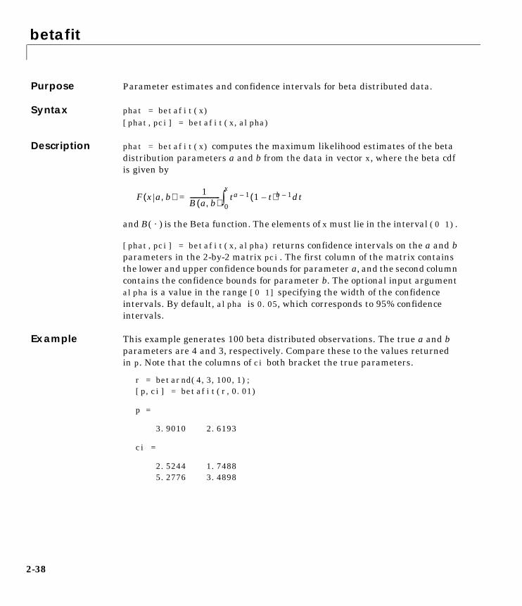
betafit
2-38
2betafitPurpose Parameter estimates and confidence intervals for beta distributed data.
Syntax phat = betafit(x)[phat,pci] = betafit(x,alpha)
Description phat = betafit(x) computes the maximum likelihood estimates of the betadistribution parameters a and b from the data in vector x, where the beta cdfis given by
and B( · ) is the Beta function. The elements of x must lie in the interval (0 1).
[phat,pci] = betafit(x,alpha) returns confidence intervals on the a and bparameters in the 2-by-2 matrix pci. The first column of the matrix containsthe lower and upper confidence bounds for parameter a, and the second columncontains the confidence bounds for parameter b. The optional input argumentalpha is a value in the range [0 1] specifying the width of the confidenceintervals. By default, alpha is 0.05, which corresponds to 95% confidenceintervals.
Example This example generates 100 beta distributed observations. The true a and bparameters are 4 and 3, respectively. Compare these to the values returnedin p. Note that the columns of ci both bracket the true parameters.
r = betarnd(4,3,100,1);[p,ci] = betafit(r,0.01)
p =
3.9010 2.6193
ci =
2.5244 1.7488 5.2776 3.4898
F x a b,( ) 1B a b,( )------------------- ta 1–
0
x
� 1 t–( )b 1– dt=
betafit
2-39
Reference Hahn, Gerald J., & Shapiro, Samuel, S. Statistical Models in Engineering.John Wiley & Sons, New York. 1994. p. 95.
See Also betalike, mle

betainv
2-40
2betainvPurpose Inverse of the beta cumulative distribution function.
Syntax X = betainv(P,A,B)
Description X = betainv(P,A,B) computes the inverse of the beta cdf with parametersspecified by A and B for the corresponding probabilities in P. Vector or matrixinputs for P, A, and B must all have the same size. A scalar input is expandedto a constant matrix with the same dimensions as the other inputs. Theparameters in A and B must all be positive, and the values in P must lie on theinterval [0 1].
The inverse beta cdf for a given probability p and a given pair of parametersa and b is
where
and B( · ) is the Beta function. Each element of output X is the value whosecumulative probability under the beta cdf defined by the correspondingparameters in A and B is specified by the corresponding value in P.
Algorithm The betainv function uses Newton’s method with modifications to constrainsteps to the allowable range for x, i.e., [0 1].
Examples p = [0.01 0.5 0.99];x = betainv(p,10,5)
x =
0.3726 0.6742 0.8981
According to this result, for a beta cdf with a=10 and b=5, a value less than orequal to 0.3726 occurs with probability 0.01. Similarly, values less than orequal to 0.6742 and 0.8981 occur with respective probabilities 0.5 and 0.99.
See Also betafit, icdf
x F 1–= p a b,( ) x:F x a b,( ) p={ }=
p F x a b,( ) 1B a b,( )------------------- ta 1–
0
x
� 1 t–( )b 1– dt= =
betalike
2-41
2betalikePurpose Negative beta log-likelihood function.
Syntax logL = betalike(params,data)[logL,avar] = betalike(params,data)
Description logL = betalike(params,data) returns the negative of the betalog-likelihood function for the beta parameters a and b specified in vectorparams and the observations specified in column vector data. The length oflogL is the length of data.
[logL,avar] = betalike(params,data) also returns avar, which is theasymptotic variance-covariance matrix of the parameter estimates if thevalues in params are the maximum likelihood estimates. avar is the inverse ofFisher’s information matrix. The diagonal elements of avar are the asymptoticvariances of their respective parameters.
betalike is a utility function for maximum likelihood estimation of the betadistribution. The likelihood assumes that all the elements in the data sampleare mutually independent. Since betalike returns the negative betalog-likelihood function, minimizing betalike using fminsearch is the same asmaximizing the likelihood.
Example This example continues the betafit example where we calculated estimates ofthe beta parameters for some randomly generated beta distributed data.
r = betarnd(4,3,100,1);[logl,avar] = betalike([3.9010 2.6193],r)
logl =
-33.0514
avar =
0.2856 0.1528 0.1528 0.1142
See Also betafit, fminsearch, gamlike, mle, weiblike

betapdf
2-42
2betapdfPurpose Beta probability density function (pdf).
Syntax Y = betapdf(X,A,B)
Description Y = betapdf(X,A,B) computes the beta pdf at each of the values in X using thecorresponding parameters in A and B. Vector or matrix inputs for X, A, and Bmust all have the same size. A scalar input is expanded to a constant matrixwith the same dimensions of the other inputs. The parameters in A and B mustall be positive, and the values in X must lie on the interval [0 1].
The beta probability density function for a given value x and given pair ofparameters a and b is
where B( · ) is the Beta function. The result, y, is the probability that a singleobservation from a beta distribution with parameters a and b will have value x.The indicator function I(0,1)(x) ensures that only values of x in the range (0 1)have nonzero probability. The uniform distribution on (0 1) is a degenerate caseof the beta pdf where a = 1 and b = 1.
A likelihood function is the pdf viewed as a function of the parameters.Maximum likelihood estimators (MLEs) are the values of the parameters thatmaximize the likelihood function for a fixed value of x.
Examples a = [0.5 1; 2 4]
a =
0.5000 1.0000 2.0000 4.0000
y = betapdf(0.5,a,a)
y = 0.6366 1.0000 1.5000 2.1875
See Also betacdf, betafit, betainv, betalike, betarnd, betastat, pdf
y f x a b,( ) 1B a b,( )-------------------xa 1– 1 x–( )b 1– I 0 1,( ) x( )= =

betarnd
2-43
2betarndPurpose Random numbers from the beta distribution.
Syntax R = betarnd(A,B)R = betarnd(A,B,m)R = betarnd(A,B,m,n)
Description R = betarnd(A,B) generates random numbers from the beta distribution withparameters specified by A and B. Vector or matrix inputs for A and B must havethe same size, which is also the size of R. A scalar input for A or B is expandedto a constant matrix with the same dimensions as the other input.
R = betarnd(A,B,m) generates a matrix of size m containing random numbersfrom the beta distribution with parameters A and B, where m is a 1-by-2 vectorcontaining the row and column dimensions of R.
R = betarnd(A,B,m,n) generates an m-by-n matrix containing randomnumbers from the beta distribution with parameters A and B.
Examples a = [1 1;2 2];b = [1 2;1 2];
r = betarnd(a,b)
r = 0.6987 0.6139 0.9102 0.8067
r = betarnd(10,10,[1 5])
r = 0.5974 0.4777 0.5538 0.5465 0.6327
r = betarnd(4,2,2,3)
r = 0.3943 0.6101 0.5768 0.5990 0.2760 0.5474
See Also betacdf, betafit, betainv, betalike, betapdf, betastat, rand, randtool

betastat
2-44
2betastatPurpose Mean and variance for the beta distribution.
Syntax [M,V] = betastat(A,B)
Description [M,V] = betastat(A,B) returns the mean and variance for the betadistribution with parameters specified by A and B. Vector or matrix inputs forA and B must have the same size, which is also the size of M and V. A scalarinput for A or B is expanded to a constant matrix with the same dimensions asthe other input.
The mean of the beta distribution with parameters a and b is andthe variance is
Examples If parameters a and b are equal, the mean is 1/2.
a = 1:6;[m,v] = betastat(a,a)
m = 0.5000 0.5000 0.5000 0.5000 0.5000 0.5000
v = 0.0833 0.0500 0.0357 0.0278 0.0227 0.0192
See Also betacdf, betafit, betainv, betalike, betapdf, betarnd
a a b+( )⁄
aba b 1+ +( ) a b+( )2
-------------------------------------------------
binocdf
2-45
2binocdfPurpose Binomial cumulative distribution function (cdf).
Syntax Y = binocdf(X,N,P)
Description binocdf(X,N,P) computes a binomial cdf at each of the values in X using thecorresponding parameters in N and P. Vector or matrix inputs for X, N, and Pmust all have the same size. A scalar input is expanded to a constant matrixwith the same dimensions of the other inputs. The values in N must all bepositive integers, and the values in X and P must lie on the interval [0 1].
The binomial cdf for a given value x and given pair of parameters n and p is
The result, y, is the probability of observing up to x successes in n independenttrials, where the probability of success in any given trial is p. The indicatorfunction I(0,1, ... ,n)(i) ensures that x only adopts values of 0, 1, ..., n.
Examples If a baseball team plays 162 games in a season and has a 50-50 chance ofwinning any game, then the probability of that team winning more than 100games in a season is:
1 – binocdf(100,162,0.5)
The result is 0.001 (i.e., 1-0.999). If a team wins 100 or more games in a season,this result suggests that it is likely that the team’s true probability of winningany game is greater than 0.5.
See Also binofit, binoinv, binopdf, binornd, binostat, cdf
y F x n p,( )ni� �
� �
i 0=
x
� piq 1 i–( )I 0 1 … n, , ,( ) i( )= =

binofit
2-46
2binofitPurpose Parameter estimates and confidence intervals for binomial data.
Syntax phat = binofit(x,n)[phat,pci] = binofit(x,n)[phat,pci] = binofit(x,n,alpha)
Description phat = binofit(x,n) returns a maximum likelihood estimate of theprobability of success in a given binomial trial based on the number ofsuccesses, x, observed in n independent trials. A scalar value for x or n isexpanded to the same size as the other input.
[phat,pci] = binofit(x,n) returns the probability estimate, phat, and the95% confidence intervals, pci.
[phat,pci] = binofit(x,n,alpha) returns the 100(1-alpha)% confidenceintervals. For example, alpha = 0.01 yields 99% confidence intervals.
Example First we generate a binomial sample of 100 elements, where the probability ofsuccess in a given trial is 0.6. Then, we estimate this probability from theoutcomes in the sample.
r = binornd(100,0.6);[phat,pci] = binofit(r,100)
phat =
0.5800
pci =
0.4771 0.6780
The 95% confidence interval, pci, contains the true value, 0.6.
Reference Johnson, N. L., S. Kotz, and A.W. Kemp, “Univariate Discrete Distributions,Second Edition,” Wiley 1992. pp. 124–130.
See Also binocdf, binoinv, binopdf, binornd, binostat, mle

binoinv
2-47
2binoinvPurpose Inverse of the binomial cumulative distribution function (cdf).
Syntax X = binoinv(Y,N,P)
Description X = binoinv(Y,N,P) returns the smallest integer X such that the binomial cdfevaluated at X is equal to or exceeds Y. You can think of Y as the probability ofobserving X successes in N independent trials where P is the probability ofsuccess in each trial. Each X is a positive integer less than or equal to N.
Vector or matrix inputs for Y, N, and P must all have the same size. A scalarinput is expanded to a constant matrix with the same dimensions as the otherinputs. The parameters in N must be positive integers, and the values in bothP and Y must lie on the interval [0 1].
Examples If a baseball team has a 50-50 chance of winning any game, what is areasonable range of games this team might win over a season of 162 games? Weassume that a surprising result is one that occurs by chance once in a decade.
binoinv([0.05 0.95],162,0.5)
ans =
71 91
This result means that in 90% of baseball seasons, a .500 team should winbetween 71 and 91 games.
See Also binocdf, binofit, binopdf, binornd, binostat, icdf
binopdf
2-48
2binopdfPurpose Binomial probability density function (pdf).
Syntax Y = binopdf(X,N,P)
Description Y = binopdf(X,N,P) computes the binomial pdf at each of the values in Xusing the corresponding parameters in N and P. Vector or matrix inputs for X,N, and P must all have the same size. A scalar input is expanded to a constantmatrix with the same dimensions of the other inputs.
The parameters in N must be positive integers, and the values in P must lie onthe interval [0 1].
The binomial probability density function for a given value x and given pair ofparameters n and p is
where q = 1-p. The result, y, is the probability of observing x successes in nindependent trials, where the probability of success in any given trial is p. Theindicator function I(0,1,...,n)(x) ensures that x only adopts values of 0, 1, ..., n.
Examples A Quality Assurance inspector tests 200 circuit boards a day. If 2% of theboards have defects, what is the probability that the inspector will find nodefective boards on any given day?
binopdf(0,200,0.02)ans =
0.0176
What is the most likely number of defective boards the inspector will find?
y = binopdf([0:200],200,0.02);[x,i] = max(y);
ii = 5
See Also binocdf, binofit, binoinv, binornd, binostat, pdf
y f x n p,( ) nx� �
� � pxq 1 x–( )I 0 1 … n, , ,( ) x( )= =

binornd
2-49
2binorndPurpose Random numbers from the binomial distribution.
Syntax R = binornd(N,P)R = binornd(N,P,mm)R = binornd(N,P,mm,nn)
Description R = binornd(N,P) generates random numbers from the binomial distributionwith parameters specified by N and P. Vector or matrix inputs for N and P musthave the same size, which is also the size of R. A scalar input for N or P isexpanded to a constant matrix with the same dimensions as the other input.
R = binornd(N,P,mm) generates a matrix of size mm containing randomnumbers from the binomial distribution with parameters N and P, where mm isa 1-by-2 vector containing the row and column dimensions of R.
R = binornd(N,p,mm,nn) generates an mm-by-nn matrix containing randomnumbers from the binomial distribution with parameters N and P.
Algorithm The binornd function uses the direct method using the definition of thebinomial distribution as a sum of Bernoulli random variables.
Examples n = 10:10:60;
r1 = binornd(n,1./n)r1 = 2 1 0 1 1 2
r2 = binornd(n,1./n,[1 6])r2 = 0 1 2 1 3 1
r3 = binornd(n,1./n,1,6)r3 = 0 1 1 1 0 3
See Also binocdf, binofit, binoinv, binopdf, binostat, rand, randtool

binostat
2-50
2binostatPurpose Mean and variance for the binomial distribution.
Syntax [M,V] = binostat(N,P)
Description [M,V] = binostat(N,P) returns the mean and variance for the binomialdistribution with parameters specified by N and P. Vector or matrix inputs forN and P must have the same size, which is also the size of M and V. A scalarinput for N or P is expanded to a constant matrix with the same dimensions asthe other input.
The mean of the binomial distribution with parameters n and p is np. Thevariance is npq, where q = 1-p.
Examples n = logspace(1,5,5)n = 10 100 1000 10000 100000
[m,v] = binostat(n,1./n)
m = 1 1 1 1 1
v = 0.9000 0.9900 0.9990 0.9999 1.0000
[m,v] = binostat(n,1/2)
m = 5 50 500 5000 50000
v =
1.0e+04 * 0.0003 0.0025 0.0250 0.2500 2.5000
See Also binocdf, binofit, binoinv, binopdf, binornd

bootstrp
2-51
2bootstrpPurpose Bootstrap statistics through resampling of data.
Syntax bootstat = bootstrp(nboot,'bootfun',d1,d2,...)[bootstat,bootsam] = bootstrp(...)
Description bootstat = bootstrp(nboot,'bootfun',d1,d2,...) draws nboot bootstrapsamples from each of the input data sets, d1, d2, etc., and passes the bootstrapsamples to function bootfun for analysis. nboot must be a positive integer, andeach input data set must contain the same number of rows, n. Each bootstrapsample contains n rows chosen randomly (with replacement) from thecorresponding input data set (d1, d2, etc.).
Each row of the output, bootstat, contains the results of applying bootfun toone set of bootstrap samples. If bootfun returns multiple outputs, only the firstis stored in bootstat. If the first output from bootfun is a matrix, the matrixis reshaped to a row vector for storage in bootstat.
[bootstat,bootsam] = bootstrap(...) returns a matrix of bootstrapindices, bootsam. Each of the nboot columns in bootsam contains indices of thevalues that were drawn from the original data sets to constitute thecorresponding bootstrap sample. For example, if d1, d2, etc., each contain 16values, and nboot = 4, then bootsam is a 16-by-4 matrix. The first columncontains the indices of the 16 values drawn from d1, d2, etc., for the first of thefour bootstrap samples, the second column contains the indices for the secondof the four bootstrap samples, and so on. (The bootstrap indices are the samefor all input data sets.)
Example Correlate the LSAT scores and law-school GPA for 15 students. These 15 datapoints are resampled to create 1000 different data sets, and the correlationbetween the two variables is computed for each dataset.
load lawdata[bootstat,bootsam] = bootstrp(1000,'corrcoef',lsat,gpa);

bootstrp
2-52
bootstat(1:5,:)
ans =
1.0000 0.3021 0.3021 1.0000 1.0000 0.6869 0.6869 1.0000 1.0000 0.8346 0.8346 1.0000 1.0000 0.8711 0.8711 1.0000 1.0000 0.8043 0.8043 1.0000
bootsam(:,1:5)
ans =
4 7 5 12 8 1 11 10 8 4 11 9 12 4 2 11 14 15 5 15 15 13 6 6 2 6 8 4 3 8 8 2 15 8 6 13 10 11 14 5 1 7 12 14 14 1 11 10 1 8 8 14 2 14 7 11 12 10 8 15 1 4 14 8 1 6 1 5 5 12 2 12 7 15 12
hist(bootstat(:,2))
0.2 0.4 0.6 0.8 10
50
100
150
200
250

bootstrp
2-53
The histogram shows the variation of the correlation coefficient across all thebootstrap samples. The sample minimum is positive, indicating that therelationship between LSAT score and GPA is not accidental.

boxplot
2-54
2boxplotPurpose Box plots of a data sample.
Syntax boxplot(X)boxplot(X,notch)boxplot(X,notch,'sym')boxplot(X,notch,'sym',vert)boxplot(X,notch,'sym',vert,whis)
Description boxplot(X) produces a box and whisker plot for each column of X. The box haslines at the lower quartile, median, and upper quartile values. The whiskersare lines extending from each end of the box to show the extent of the rest ofthe data. Outliers are data with values beyond the ends of the whiskers. Ifthere is no data outside the whisker, a dot is placed at the bottom whisker.
boxplot(X,notch) with notch = 1 produces a notched-box plot. Notches grapha robust estimate of the uncertainty about the means for box-to-boxcomparison. The default, notch = 0, produces a rectangular box plot.
boxplot(X,notch,'sym') where sym is a plotting symbol, affords control of thesymbol for outliers. The default is '+'. See MATLAB’s LineSpec property forinformation about the available marker symbols.
boxplot(X,notch,'sym',vert) with vert = 0 creates horizontal boxes ratherthan the default vertical boxes (vert = 1).
boxplot(X,notch,'sym',vert,whis) enables you to specify the length of the“whiskers.” whis defines the length of the whiskers as a function of theinter-quartile range (default = 1.5 * IQR). If whis = 0, then boxplot displays alldata values outside the box using the plotting symbol, 'sym'.
Examples x1 = normrnd(5,1,100,1);x2 = normrnd(6,1,100,1);x = [x1 x2];boxplot(x,1)
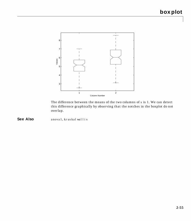
boxplot
2-55
The difference between the means of the two columns of x is 1. We can detectthis difference graphically by observing that the notches in the boxplot do notoverlap.
See Also anova1, kruskalwallis
1 2
3
4
5
6
7
8
Val
ues
Column Number

capable
2-56
2capablePurpose Process capability indices.
Syntax p = capable(data,specs)[p,Cp,Cpk] = capable(data,specs)
Description p = capable(data,specs) computes the probability that a sample, data, fromsome process falls outside the bounds specified in specs, a 2-element vector ofthe form [lower upper].
The assumptions are that the measured values in the vector data are normallydistributed with constant mean and variance and that the measurements arestatistically independent.
[p,Cp,Cpk] = capable(data,specs) additionally returns the capabilityindices Cp and Cpk.
Cp is the ratio of the range of the specifications to six times the estimate of theprocess standard deviation:
For a process that has its average value on target, a Cp of 1 translates to a littlemore than one defect per thousand. Recently, many industries have set aquality goal of one part per million. This would correspond to Cp = 1.6. Thehigher the value of Cp, the more capable the process.
Cpk is the ratio of difference between the process mean and the closerspecification limit to three times the estimate of the process standarddeviation:
where the process mean is µ. For processes that do not maintain their averageon target, Cpk is a more descriptive index of process capability.
Example Imagine a machined part with specifications requiring a dimension to bewithin three thousandths of an inch of nominal. Suppose that the machiningprocess cuts too thick by one thousandth of an inch on average and also has a
CpUSL LSL–
6σ--------------------------------=
Cpk min USL µ–3σ
-----------------------µ LSL–
3σ----------------------,� �
� �=

capable
2-57
standard deviation of one thousandth of an inch. What are the capabilityindices of this process?
data = normrnd(1,1,30,1);[p,Cp,Cpk] = capable(data,[-3 3]);
indices = [p Cp Cpk]indices =
0.0172 1.1144 0.7053
We expect 17 parts out of a thousand to be out-of-specification. Cpk is less thanCp because the process is not centered.
Reference Montgomery, D., “Introduction to Statistical Quality Control,” John Wiley &Sons 1991. pp. 369–374.
See Also capaplot, histfit
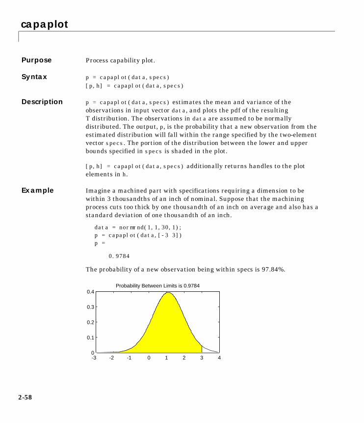
capaplot
2-58
2capaplotPurpose Process capability plot.
Syntax p = capaplot(data,specs)[p,h] = capaplot(data,specs)
Description p = capaplot(data,specs) estimates the mean and variance of theobservations in input vector data, and plots the pdf of the resultingT distribution. The observations in data are assumed to be normallydistributed. The output, p, is the probability that a new observation from theestimated distribution will fall within the range specified by the two-elementvector specs. The portion of the distribution between the lower and upperbounds specified in specs is shaded in the plot.
[p,h] = capaplot(data,specs) additionally returns handles to the plotelements in h.
Example Imagine a machined part with specifications requiring a dimension to bewithin 3 thousandths of an inch of nominal. Suppose that the machiningprocess cuts too thick by one thousandth of an inch on average and also has astandard deviation of one thousandth of an inch.
data = normrnd(1,1,30,1);p = capaplot(data,[-3 3])p =
0.9784
The probability of a new observation being within specs is 97.84%.
-3 -2 -1 0 1 2 3 40
0.1
0.2
0.3
0.4Probability Between Limits is 0.9784

capaplot
2-59
See Also capable, histfit

caseread
2-60
2casereadPurpose Read casenames from a file.
Syntax names = caseread('filename')names = caseread
Description names = caseread('filename') reads the contents of filename and returns astring matrix of names. filename is the name of a file in the current directory,or the complete pathname of any file elsewhere. caseread treats each line as aseparate case.
names = caseread displays the Select File to Open dialog box for interactiveselection of the input file.
Example Read the file months.dat created using the function casewrite on the nextpage.
type months.dat
JanuaryFebruaryMarchAprilMay
names = caseread('months.dat')names =
January FebruaryMarch April May
See Also tblread, gname, casewrite, tdfread
casewrite
2-61
2casewritePurpose Write casenames from a string matrix to a file.
Syntax casewrite(strmat,'filename')casewrite(strmat)
Description casewrite(strmat,'filename') writes the contents of string matrix strmatto filename. Each row of strmat represents one casename. filename is thename of a file in the current directory, or the complete pathname of any fileelsewhere. casewrite writes each name to a separate line in filename.
casewrite(strmat) displays the Select File to Write dialog box for interactivespecification of the output file.
Example strmat = str2mat('January','February','March','April','May')
strmat =
January FebruaryMarch April May
casewrite(strmat,'months.dat')type months.dat
January FebruaryMarch April May
See Also gname, caseread, tblwrite, tdfread

cdf
2-62
2cdfPurpose Computes a chosen cumulative distribution function (cdf).
Syntax P = cdf('name',X,A1,A2,A3)
Description P = cdf('name',X,A1,A2,A3) returns a matrix of probabilities, where name isa string containing the name of the distribution, X is a matrix of values, and A,A2, and A3 are matrices of distribution parameters. Depending on thedistribution, some of these parameters may not be necessary.
Vector or matrix inputs for X, A1, A2, and A3 must have the same size, which isalso the size of P. A scalar input for X, A1, A2, or A3 is expanded to a constantmatrix with the same dimensions as the other inputs.
cdf is a utility routine allowing you to access all the cdfs in the StatisticsToolbox by using the name of the distribution as a parameter. See “Overviewof the Distributions” on page 1-12 for the list of available distributions.
Examples p = cdf('Normal',-2:2,0,1)p =
0.0228 0.1587 0.5000 0.8413 0.9772
p = cdf('Poisson',0:5,1:6)p =
0.3679 0.4060 0.4232 0.4335 0.4405 0.4457
See Also betacdf, binocdf, chi2cdf, expcdf, fcdf, gamcdf, geocdf, hygecdf, icdf,logncdf, mle, nbincdf, ncfcdf, nctcdf, ncx2cdf, normcdf, pdf, poisscdf,random, raylcdf, tcdf, unidcdf, unifcdf, weibcdf

cdfplot
2-63
2cdfplotPurpose Plot of empirical cumulative distribution function.
Syntax cdfplot(X)h = cdfplot(X)[h,stats] = cdfplot(X)
Description cdfplot(X) displays a plot of the empirical cumulative distribution function(cdf) for the data in the vector X. The empirical cdf is defined as theproportion of X values less than or equal to x.
This plot, like those produced by hist and normplot, is useful for examiningthe distribution of a sample of data. You can overlay a theoretical cdf on thesame plot to compare the empirical distribution of the sample to the theoreticaldistribution.
The kstest, kstest2, and lillietest functions compute test statistics thatare derived from the empirical cdf. You may find the empirical cdf plotproduced by cdfplot useful in helping you to understand the output from thosefunctions.
H = cdfplot(X) returns a handle to the cdf curve.
[h,stats] = cdfplot(X) also returns a stats structure with the followingfields.
Examples Generate a normal sample and an empirical cdf plot of the data.
x = normrnd(0,1,50,1);cdfplot(x)
Field Contents
stats.min Minimum value
stats.max Maximum value
stats.mean Sample mean
stats.median Sample median (50th percentile)
stats.std Sample standard deviation
F x( )

cdfplot
2-64
See Also hist, kstest, kstest2, lillietest, normplot
−3 −2 −1 0 1 2 30
0.1
0.2
0.3
0.4
0.5
0.6
0.7
0.8
0.9
1
x
F(x
)
Empirical CDF

chi2cdf
2-65
2chi2cdfPurpose Chi-square (χ2) cumulative distribution function (cdf).
Syntax P = chi2cdf(X,V)
Description P = chi2cdf(X,V) computes the χ2 cdf at each of the values in X using thecorresponding parameters in V. Vector or matrix inputs for X and V must havethe same size. A scalar input is expanded to a constant matrix with the samedimensions as the other input. The degrees of freedom parameters in V must bepositive integers, and the values in X must lie on the interval [0 1].
The χ2 cdf for a given value x and degrees-of-freedom ν is
where Γ( · ) is the Gamma function. The result, p, is the probability that asingle observation from a χ2 distribution with ν degrees of freedom will fall inthe interval [0 x].
The χ2 density function with ν degrees-of-freedom is the same as the gammadensity function with parameters ν/2 and 2.
Examples probability = chi2cdf(5,1:5)probability =
0.9747 0.9179 0.8282 0.7127 0.5841
probability = chi2cdf(1:5,1:5)probability =
0.6827 0.6321 0.6084 0.5940 0.5841
See Also cdf, chi2inv, chi2pdf, chi2rnd, chi2stat
p F x ν( ) t ν 2–( ) 2⁄ e t– 2⁄
2ν 2⁄ Γ ν 2⁄( )-----------------------------------
0
x
� dt= =

chi2inv
2-66
2chi2invPurpose Inverse of the chi-square (χ2) cumulative distribution function (cdf).
Syntax X = chi2inv(P,V)
Description X = chi2inv(P,V) computes the inverse of the χ2 cdf with parametersspecified by V for the corresponding probabilities in P. Vector or matrix inputsfor P and V must have the same size. A scalar input is expanded to a constantmatrix with the same dimensions as the other inputs.
The degrees of freedom parameters in V must be positive integers, and thevalues in P must lie in the interval [0 1].
The inverse χ2 cdf for a given probability p and ν degrees of freedom is
where
and Γ( · ) is the Gamma function. Each element of output X is the value whosecumulative probability under the χ2 cdf defined by the corresponding degreesof freedom parameter in V is specified by the corresponding value in P.
Examples Find a value that exceeds 95% of the samples from a χ2 distribution with10 degrees of freedom.
x = chi2inv(0.95,10)x =
18.3070
You would observe values greater than 18.3 only 5% of the time by chance.
See Also chi2cdf, chi2pdf, chi2rnd, chi2stat, icdf
x F 1– p ν( ) x:F x ν( ) p={ }= =
p F x ν( ) t ν 2–( ) 2⁄ e t– 2⁄
2ν 2⁄ Γ ν 2⁄( )-----------------------------------
0
x
� dt= =

chi2pdf
2-67
2chi2pdfPurpose Chi-square (χ2) probability density function (pdf).
Syntax Y = chi2pdf(X,V)
Description Y = chi2pdf(X,V) computes the χ2 pdf at each of the values in X using thecorresponding parameters in V. Vector or matrix inputs for X and V must havethe same size, which is also the size of output Y. A scalar input is expanded toa constant matrix with the same dimensions as the other input.
The degrees of freedom parameters in V must be positive integers, and thevalues in X must lie on the interval [0 1].
The χ2 pdf for a given value x and ν degrees of freedom is
where Γ( · ) is the Gamma function. The result, y, is the probability that asingle observation from a χ2 distribution with ν degrees of freedom will havevalue x.
If x is standard normal, then x2 is distributed χ2 with one degree of freedom. Ifx1, x2, ..., xn are n independent standard normal observations, then the sum ofthe squares of the x’s is distributed χ2 with n degrees of freedom (and isequivalent to the gamma density function with parameters ν/2 and 2).
Examples nu = 1:6;x = nu;y = chi2pdf(x,nu)
y =
0.2420 0.1839 0.1542 0.1353 0.1220 0.1120
The mean of the χ2 distribution is the value of the degrees of freedomparameter, nu. The above example shows that the probability density of themean falls as nu increases.
See Also chi2cdf, chi2inv, chi2rnd, chi2stat, pdf
y f x ν( ) x ν 2–( ) 2⁄ e x– 2⁄
2ν 2⁄ Γ ν 2⁄( )-------------------------------------= =

chi2rnd
2-68
2chi2rndPurpose Random numbers from the chi-square (χ2) distribution.
Syntax R = chi2rnd(V)R = chi2rnd(V,m)R = chi2rnd(V,m,n)
Description R = chi2rnd(V) generates random numbers from the χ2 distribution withdegrees of freedom parameters specified by V. R is the same size as V.
R = chi2rnd(V,m) generates a matrix of size m containing random numbersfrom the χ2 distribution with degrees of freedom parameter V, where m is a1-by-2 vector containing the row and column dimensions of R.
R = chi2rnd(V,m,n) generates an m-by-n matrix containing random numbersfrom the χ2 distribution with degrees of freedom parameter V.
Examples Note that the first and third commands are the same, but are different from thesecond command.
r = chi2rnd(1:6)r =
0.0037 3.0377 7.8142 0.9021 3.2019 9.0729
r = chi2rnd(6,[1 6])r =
6.5249 2.6226 12.2497 3.0388 6.3133 5.0388
r = chi2rnd(1:6,1,6)r =
0.7638 6.0955 0.8273 3.2506 1.5469 10.9197
See Also chi2cdf, chi2inv, chi2pdf, chi2stat

chi2stat
2-69
2chi2statPurpose Mean and variance for the chi-square (χ2) distribution.
Syntax [M,V] = chi2stat(NU)
Description [M,V] = chi2stat(NU) returns the mean and variance for the χ2 distributionwith degrees of freedom parameters specified by NU.
The mean of the χ2 distribution is ν, the degrees of freedom parameter, and thevariance is 2ν.
Example nu = 1:10;nu = nu'∗nu;[m,v] = chi2stat(nu)
m =
1 2 3 4 5 6 7 8 9 10 2 4 6 8 10 12 14 16 18 20 3 6 9 12 15 18 21 24 27 30 4 8 12 16 20 24 28 32 36 40 5 10 15 20 25 30 35 40 45 50 6 12 18 24 30 36 42 48 54 60 7 14 21 28 35 42 49 56 63 70 8 16 24 32 40 48 56 64 72 80 9 18 27 36 45 54 63 72 81 9010 20 30 40 50 60 70 80 90 100
v =
2 4 6 8 10 12 14 16 18 20 4 8 12 16 20 24 28 32 36 40 6 12 18 24 30 36 42 48 54 60 8 16 24 32 40 48 56 64 72 8010 20 30 40 50 60 70 80 90 10012 24 36 48 60 72 84 96 108 12014 28 42 56 70 84 98 112 126 14016 32 48 64 80 96 112 128 144 16018 36 54 72 90 108 126 144 162 18020 40 60 80 100 120 140 160 180 200
See Also chi2cdf, chi2inv, chi2pdf, chi2rnd

classify
2-70
2classifyPurpose Linear discriminant analysis.
Syntax class = classify(sample,training,group)
Description class = classify(sample,training,group) assigns each row of the data insample to one of the groups into which the training set, training, is alreadydivided. sample and training must have the same number of columns.
The vector group contains integers, from one to the number of groups, thatidentify the group to which each row of the training set belongs. group andtraining must have the same number of rows.
The function returns class, a vector with the same number of rows as sample.Each element of class identifies the group to which the corresponding elementof sample has been assigned. The classify function determines the group intowhich each row in sample is classified by computing the Mahalanobis distancebetween each row in sample and each row in training.
Example load discrimsample = ratings(idx,:);training = ratings(1:200,:);g = group(1:200);class = classify(sample,training,g);first5 = class(1:5)
first5 =
2 2 2 2 2
See Also mahal

cluster
2-71
2clusterPurpose Construct clusters from linkage output.
Syntax T = cluster(Z,cutoff)T = cluster(Z,cutoff,depth,flag)
Description T = cluster(Z,cutoff) constructs clusters from the hierarchical clustertree, Z, generated by the linkage function. Z is a matrix of size (m-1)-by-3,where m is the number of observations in the original data.
cutoff is a threshold value that determines how the cluster function createsclusters. The value of cutoff determines how cluster interprets it.
T = cluster(Z,cutoff,depth,flag) constructs clusters from cluster tree Z.The depth argument specifies the number of levels in the hierarchical clustertree to include in the inconsistency coefficient computation. (The inconsistencycoefficient compares a link between two objects in the cluster tree withneighboring links up to a specified depth. See the inconsistent function formore information.) When the depth argument is specified, cutoff is alwaysinterpreted as the inconsistency coefficient threshold.
The flag argument overrides the default meaning of the cutoff argument. Ifflag is 'inconsistent', then cutoff is interpreted as a threshold for theinconsistency coefficient. If flag is 'clusters', then cutoff is the maximumnumber of clusters.
Value Meaning
0 < cutoff < 2 cutoff is interpreted as the threshold for theinconsistency coefficient. The inconsistency coefficientquantifies the degree of difference between objects inthe hierarchical cluster tree. If the inconsistencycoefficient of a link is greater than the threshold, thecluster function uses the link as a boundary for acluster grouping. For more information about theinconsistency coefficient, see the inconsistentfunction.
cutoff >= 2 cutoff is interpreted as the maximum number ofclusters to retain in the hierarchical tree.

cluster
2-72
The output, T, is a vector of size m that identifies, by number, the cluster inwhich each object was grouped. To find out which objects from the originaldataset are contained in cluster i, use find(T==i).
Example The example uses the pdist function to calculate the distance between itemsin a matrix of random numbers and then uses the linkage function to computethe hierarchical cluster tree based on the matrix. The output of the linkagefunction is passed to the cluster function. The cutoff value 3 indicates thatyou want to group the items into three clusters. The example uses the findfunction to list all the items grouped into cluster 2.
rand('seed', 0); X = [rand(10,3); rand(10,3)+1; rand(10,3)+2]; Y = pdist(X); Z = linkage(Y); T = cluster(Z,3); find(T==3)
ans = 11121314151617181920
See Also clusterdata, cophenet, dendrogram, inconsistent, linkage, pdist,squareform
clusterdata
2-73
2clusterdataPurpose Construct clusters from data.
Syntax T = clusterdata(X,cutoff)
Description T = clusterdata(X,cutoff) constructs clusters from the data matrix X. X is amatrix of size m by n, interpreted as m observations of n variables.
cutoff is a threshold value that determines how the cluster function createsclusters. The value of cutoff determines how clusterdata interprets it.
The output, T, is a vector of size m that identifies, by number, the cluster inwhich each object was grouped.
T = clusterdata(X,cutoff) is the same as
Y = pdist(X,'euclid');Z = linkage(Y,'single');T = cluster(Z,cutoff);
Follow this sequence to use nondefault parameters for pdist and linkage.
Example The example first creates a sample dataset of random numbers. The examplethen uses the clusterdata function to compute the distances between items inthe dataset and create a hierarchical cluster tree from the dataset. Finally, theclusterdata function groups the items in the dataset into three clusters. Theexample uses the find function to list all the items in cluster 2.
Value Meaning
0 < cutoff < 1 cutoff is interpreted as the threshold for theinconsistency coefficient. The inconsistency coefficientquantifies the degree of difference between objects inthe hierarchical cluster tree. If the inconsistencycoefficient of a link is greater than the threshold, thecluster function uses the link as a boundary for acluster grouping. For more information about theinconsistency coefficient, see the inconsistentfunction.
cutoff >= 1 cutoff is interpreted as the maximum number ofclusters to retain in the hierarchical tree.

clusterdata
2-74
rand('seed',12); X = [rand(10,3); rand(10,3)+1.2; rand(10,3)+2.5; T = clusterdata(X,3); find(T==2)
ans = 21 22 23 24 25 26 27 28 29 30
See Also cluster, cophenet, dendrogram, inconsistent, linkage, pdist, squareform

combnk
2-75
2combnkPurpose Enumeration of all combinations of n objects k at a time.
Syntax C = combnk(v,k)
Description C = combnk(v,k) returns all combinations of the n elements in v taken k at atime.
C = combnk(v,k) produces a matrix C with k columns and n! / k!(n-k)! rows,where each row contains k of the elements in the vector v.
It is not practical to use this function if v has more than about 15 elements.
Example Combinations of characters from a string.
C = combnk('tendril',4);last5 = C(31:35,:)
last5 =
tedrtenltenitenrtend
Combinations of elements from a numeric vector.
c = combnk(1:4,2)
c = 3 4 2 4 2 3 1 4 1 3 1 2

cophenet
2-76
2cophenetPurpose Cophenetic correlation coefficient.
Syntax c = cophenet(Z,Y)
Description c = cophenet(Z,Y) computes the cophenetic correlation coefficient whichcompares the distance information in Z, generated by linkage, and thedistance information in Y, generated by pdist. Z is a matrix of size (m-1)-by-3,with distance information in the third column. Y is a vector of size
.
For example, given a group of objects {1, 2, ..., m} with distances Y, the functionlinkage produces a hierarchical cluster tree. The cophenet function measuresthe distortion of this classification, indicating how readily the data fits into thestructure suggested by the classification.
The output value, c, is the cophenetic correlation coefficient. The magnitude ofthis value should be very close to 1 for a high-quality solution. This measurecan be used to compare alternative cluster solutions obtained using differentalgorithms.
The cophenetic correlation between Z(:,3) and Y is defined as
where:
• Yij is the distance between objects i and j in Y.
• Zij is the distance between objects i and j in Z(:,3).
• y and z are the average of Y and Z(:,3), respectively.
Example rand('seed',12); X = [rand(10,3);rand(10,3)+1;rand(10,3)+2];Y = pdist(X);Z = linkage(Y,'centroid');c = cophenet(Z,Y)
c = 0.6985
m m 1–( ) 2⁄⋅
cΣi j< Yij y–( ) Zij z–( )
Σi j< Yij y–( )2Σi j< Zij z–( )2------------------------------------------------------------------------------=

cophenet
2-77
See Also cluster, dendrogram, inconsistent, linkage, pdist, squareform

cordexch
2-78
2cordexchPurpose D-optimal design of experiments – coordinate exchange algorithm.
Syntax settings = cordexch(nfactors,nruns)[settings,X] = cordexch(nfactors,nruns)[settings,X] = cordexch(nfactors,nruns,'model')
Description settings = cordexch(nfactors,nruns) generates the factor settings matrix,settings, for a D-optimal design using a linear additive model with a constantterm. settings has nruns rows and nfactors columns.
[settings,X] = cordexch(nfactors,nruns) also generates the associateddesign matrix X.
[settings,X] = cordexch(nfactors,nruns,'model') produces a design forfitting a specified regression model. The input, 'model', can be one of thesestrings:
• 'interaction' – includes constant, linear, and cross-product terms.
• 'quadratic' – includes interactions and squared terms.
• 'purequadratic' – includes constant, linear and squared terms.
Example The D-optimal design for two factors in nine run using a quadratic model is the32 factorial as shown below:
settings = cordexch(2,9,'quadratic')
settings =
-1 1 1 1 0 1 1 -1 -1 -1 0 -1 1 0 0 0 -1 0
See Also rowexch, daugment, dcovary, hadamard, fullfact, ff2n
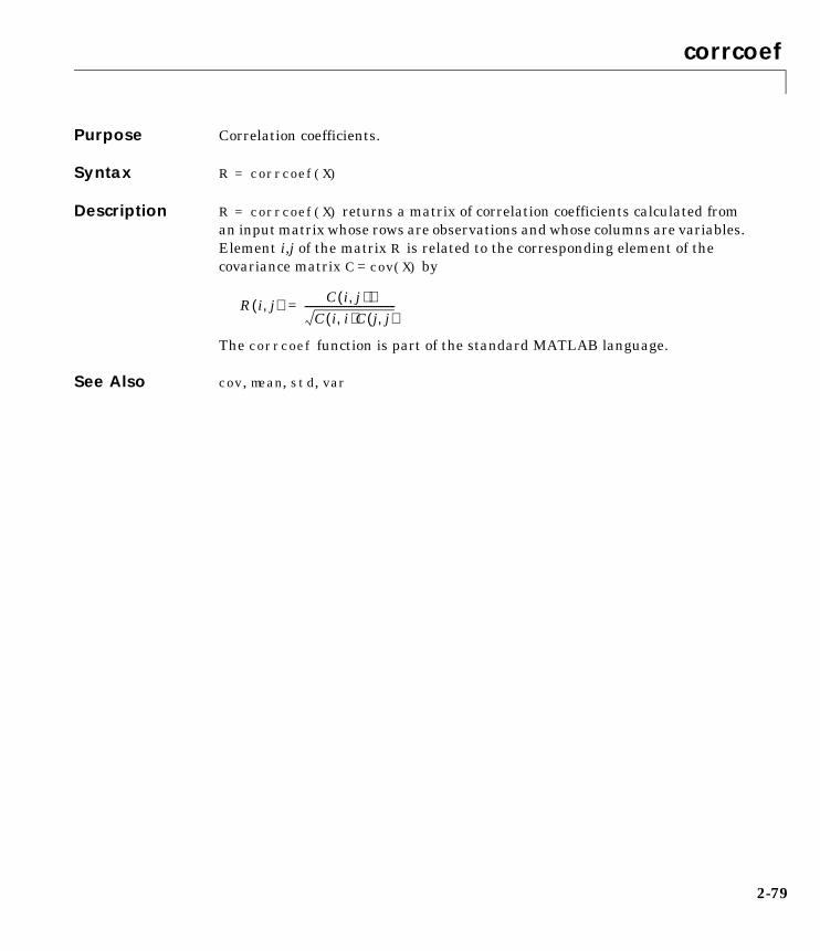
corrcoef
2-79
2corrcoefPurpose Correlation coefficients.
Syntax R = corrcoef(X)
Description R = corrcoef(X) returns a matrix of correlation coefficients calculated froman input matrix whose rows are observations and whose columns are variables.Element i,j of the matrix R is related to the corresponding element of thecovariance matrix C = cov(X) by
The corrcoef function is part of the standard MATLAB language.
See Also cov, mean, std, var
R i j,( ) C i j ),( )C i i,( )C j j,( )
-------------------------------------=

cov
2-80
2covPurpose Covariance matrix.
Syntax C = cov(X)C = cov(x,y)
Description C = cov(X) computes the covariance matrix. For a single vector, cov(x)returns a scalar containing the variance. For matrices, where each row is anobservation, and each column a variable, cov(X) is the covariance matrix.
The variance function, var(X) is the same as diag(cov(X)).
The standard deviation function, std(X) is equivalent to sqrt(diag(cov(X))).
cov(x,y), where x and y are column vectors of equal length, gives the sameresult as cov([x y]).
The cov function is part of the standard MATLAB language.
Algorithm The algorithm for cov is
[n,p] = size(X);X = X - ones(n,1) * mean(X);Y = X'∗X/(n-1);
See Also corrcoef, mean, std, var
xcov, xcorr (Signal Processing Toolbox)
crosstab
2-81
2crosstabPurpose Cross-tabulation of several vectors.
Syntax table = crosstab(col1,col2)table = crosstab(col1,col2,col3,...)[table,chi2,p] = crosstab(col1,col2)[table,chi2,p,label] = crosstab(col1,col2)
Description table = crosstab(col1,col2) takes two vectors of positive integers andreturns a matrix, table, of cross-tabulations. The ijth element of tablecontains the count of all instances where col1 = i and col2 = j.
Alternatively, col1 and col2 can be vectors containing noninteger values,character arrays, or cell arrays of strings. crosstab implicitly assigns apositive integer group number to each distinct value in col1 and col2, andcreates a cross-tabulation using those numbers.
table = crosstab(col1,col2,col3,...) returns table as an n-dimensionalarray, where n is the number of arguments you supply. The value oftable(i,j,k,...) is the count of all instances where col1 = i, col2 = j,col3 = k, and so on.
[table,chi2,p] = crosstab(col1,col2) also returns the chi-square statistic,chi2, for testing the independence of the rows and columns of table. Thescalar p is the significance level of the test. Values of p near zero cast doubt onthe assumption of independence of the rows and columns of table.
[table,chi2,p,label] = crosstab(col1,col2) also returns a cell arraylabel that has one column for each input argument. The value in label(i,j)is the value of colj that defines group i in the jth dimension.
Example Example 1We generate 2 columns of 50 discrete uniform random numbers. The firstcolumn has numbers from 1 to 3. The second has only the numbers 1 and 2. Thetwo columns are independent so we would be surprised if p were near zero.
r1 = unidrnd(3,50,1);r2 = unidrnd(2,50,1);[table,chi2,p] = crosstab(r1,r2)

crosstab
2-82
table =
10 5 8 8 6 13
chi2 =
4.1723
p =
0.1242
The result, 0.1242, is not a surprise. A very small value of p would make ussuspect the “randomness” of the random number generator.
Example 2We have data collected on several cars over a period of time. How manyfour-cylinder cars were made in the USA during the late part of this period?
[t,c,p,l] = crosstab(cyl4,when,org);
ll = 'Other' 'Early' 'USA' 'Four' 'Mid' 'Europe' [] 'Late' 'Japan'
t(2,3,1)
ans = 38
See Also tabulate

daugment
2-83
2daugmentPurpose D-optimal augmentation of an experimental design.
Syntax settings = daugment(startdes,nruns)[settings,X] = daugment(startdes,nruns,'model')
Description settings = daugment(startdes,nruns) augments an initial experimentaldesign, startdes, with nruns new tests.
[settings,X] = daugment(startdes,nruns,'model') also supplies thedesign matrix, X. The input, 'model', controls the order of the regressionmodel. By default, daugment assumes a linear additive model. Alternatively,'model' can be any of these:
• 'interaction' – includes constant, linear, and cross product terms.
• 'quadratic' – includes interactions plus squared terms.
• 'purequadratic' – includes constant, linear, and squared terms.
daugment uses the coordinate exchange algorithm.
Example We add 5 runs to a 22 factorial design to allow us to fit a quadratic model.
startdes = [-1 -1; 1 -1; -1 1; 1 1];settings = daugment(startdes,5,'quadratic')
settings =
-1 -1 1 -1 -1 1 1 1 1 0 -1 0 0 1 0 0 0 -1
The result is a 32 factorial design.
See Also cordexch, dcovary, rowexch

dcovary
2-84
2dcovaryPurpose D-optimal design with specified fixed covariates.
Syntax settings = dcovary(factors,covariates)[settings,X] = dcovary(factors,covariates,'model')
Description settings = dcovary(factors,covariates,'model') creates a D-optimaldesign subject to the constraint of fixed covariates for each run. factors isthe number of experimental variables you want to control.
[settings,X] = dcovary(factors,covariates,'model') also creates theassociated design matrix, X. The input, 'model', controls the order of theregression model. By default, dcovary assumes a linear additive model.Alternatively, 'model' can be any of these:
• 'interaction' – includes constant, linear, and cross product terms.
• 'quadratic' – includes interactions plus squared terms.
• 'purequadratic' – includes constant, linear, and squared terms.
Example Suppose we want to block an eight run experiment into 4 blocks of size 2 to fita linear model on two factors.
covariates = dummyvar([1 1 2 2 3 3 4 4]);settings = dcovary(2,covariates(:,1:3),'linear')settings =
1 1 1 0 0 -1 -1 1 0 0 -1 1 0 1 0 1 -1 0 1 0 1 1 0 0 1 -1 -1 0 0 1 -1 1 0 0 0 1 -1 0 0 0
The first two columns of the output matrix contain the settings for the twofactors. The last three columns are dummy variable codings for the four blocks.
See Also daugment, cordexch

dendrogram
2-85
2dendrogramPurpose Plot dendrogram graphs.
Syntax H = dendrogram(Z) H = dendrogram(Z,p)[H,T] = dendrogram(...)
Description H = dendrogram(Z) generates a dendrogram plot of the hierarchical, binarycluster tree, Z. Z is an (m-1)-by-3 matrix, generated by the linkage function,where m is the number of objects in the original dataset.
A dendrogram consists of many upside-down, U-shaped lines connectingobjects in a hierarchical tree. Except for the Ward linkage (see linkage), theheight of each U represents the distance between the two objects beingconnected. The output, H, is a vector of line handles.
H = dendrogram(Z,p) generates a dendrogram with only the top p nodes. Bydefault, dendrogram uses 30 as the value of p. When there are more than 30initial nodes, a dendrogram may look crowded. To display every node, set p = 0.
[H,T] = dendrogram(...) generates a dendrogram and returns T, a vector ofsize m that contains the cluster number for each object in the original dataset.T provides access to the nodes of a cluster hierarchy that are not displayed inthe dendrogram because they fall below the cutoff value p. For example, to findout which objects are contained in leaf node k of the dendrogram, usefind(T==k). Leaf nodes are the nodes at the bottom of the dendrogram thathave no other nodes below them.
When there are fewer than p objects in the original data, all objects aredisplayed in the dendrogram. In this case, T is the identical map, i.e.,T = (1:m)', where each node contains only itself.
Example rand('seed',12); X= rand(100,2); Y= pdist(X,'citiblock'); Z= linkage(Y,'average'); [H, T] = dendrogram(Z);

dendrogram
2-86
find(T==20)
ans =
204962657396
This output indicates that leaf node 20 in the dendrogram contains the originaldata points 20, 49, 62, 65, 73, and 96.
See Also cluster, clusterdata, cophenet, inconsistent, linkage, pdist, squareform
0
0.1
0.2
0.3
0.4
0.5
0.6
0.7
14 17 13 22 12 8 23 20 19 1 21 15 5 2 3 16 27 4 18 24 28 6 10 7 30 26 9 25 11 29

disttool
2-87
2disttoolPurpose Interactive graph of cdf (or pdf) for many probability distributions.
Syntax disttool
Description The disttool command displays a graphic user interface for exploring theeffects of changing parameters on the plot of a cdf or pdf. Clicking and dragginga vertical line on the plot allows you to interactively evaluate the function overits entire domain.
Evaluate the plotted function by typing a value in the x-axis edit box ordragging the vertical reference line on the plot. For cdfs, you can evaluate theinverse function by typing a value in the y-axis edit box or dragging thehorizontal reference line on the plot. The shape of the pointer changes from anarrow to a crosshair when it is over the vertical or horizontal line to indicatethat the reference line is draggable.
To change the distribution function, choose an option from the menu offunctions at the top left of the figure. To change from cdfs to pdfs, choose anoption from the menu at the top right of the figure.
To change the parameter settings, move the sliders or type a value in the editbox under the name of the parameter. To change the limits of a parameter, typea value in the edit box at the top or bottom of the parameter slider.
To close the tool, press the Close button.
See Also randtool

dummyvar
2-88
2dummyvarPurpose Matrix of 0-1 “dummy” variables.
Syntax D = dummyvar(group)
Description D = dummyvar(group) generates a matrix, D, of 0-1 columns. D has one columnfor each unique value in each column of the matrix group. Each column ofgroup contains positive integers that indicate the group membership of anindividual row.
Example Suppose we are studying the effects of two machines and three operators on aprocess. The first column of group would have the values 1 or 2 depending onwhich machine was used. The second column of group would have the values1, 2, or 3 depending on which operator ran the machine.
group = [1 1;1 2;1 3;2 1;2 2;2 3];D = dummyvar(group)
D = 1 0 1 0 0 1 0 0 1 0 1 0 0 0 1 0 1 1 0 0 0 1 0 1 0 0 1 0 0 1
See Also pinv, regress

errorbar
2-89
2errorbarPurpose Plot error bars along a curve.
Syntax errorbar(X,Y,L,U,symbol)errorbar(X,Y,L)errorbar(Y,L)
Description errorbar(X,Y,L,U,symbol) plots X versus Y with error bars specified by Land U. X, Y, L, and U must be the same length. If X, Y, L, and U are matrices, theneach column produces a separate line. The error bars are each drawn a distanceof U(i) above and L(i) below the points in (X,Y). symbol is a string thatcontrols the line type, plotting symbol, and color of the error bars.
errorbar(X,Y,L) plots X versus Y with symmetric error bars about Y.
errorbar(Y,L) plots Y with error bars [Y–L Y+L].
The errorbar function is a part of the standard MATLAB language.
Example lambda = (0.1:0.2:0.5);r = poissrnd(lambda(ones(50,1),:));[p,pci] = poissfit(r,0.001);L = p - pci(1,:) U = pci(2,:) - perrorbar(1:3,p,L,U,'+')
L = 0.1200 0.1600 0.2600
U = 0.2000 0.2200 0.3400
0.5 1 1.5 2 2.5 3 3.50
0.2
0.4
0.6
0.8

ewmaplot
2-90
2ewmaplotPurpose Exponentially Weighted Moving Average (EWMA) chart for Statistical ProcessControl (SPC).
Syntax ewmaplot(data)ewmaplot(data,lambda)ewmaplot(data,lambda,alpha)ewmaplot(data,lambda,alpha,specs)h = ewmaplot(...)
Description ewmaplot(data) produces an EWMA chart of the grouped responses in data.The rows of data contain replicate observations taken at a given time. The rowsshould be in time order.
ewmaplot(data,lambda) produces an EWMA chart of the grouped responses indata, and specifies how much the current prediction is influenced by pastobservations. Higher values of lambda give more weight to past observations.By default, lambda = 0.4; lambda must be between 0 and 1.
ewmaplot(data,lambda,alpha) produces an EWMA chart of the groupedresponses in data, and specifies the significance level of the upper and lowerplotted confidence limits. alpha is 0.0027 by default. This value producesthree-sigma limits:
norminv(1-0.0027/2)
ans =3
To get k-sigma limits, use the expression 2*(1-normcdf(k)). For example, thecorrect alpha value for 2-sigma limits is 0.0455, as shown below.
k = 2;2*(1-normcdf(k))
ans = 0.0455
ewmaplot(data,lambda,alpha,specs) produces an EWMA chart of thegrouped responses in data, and specifies a two-element vector, specs, for thelower and upper specification limits of the response.
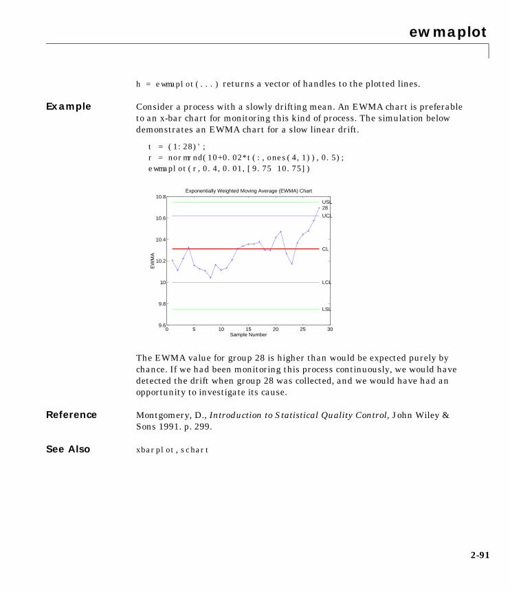
ewmaplot
2-91
h = ewmaplot(...) returns a vector of handles to the plotted lines.
Example Consider a process with a slowly drifting mean. An EWMA chart is preferableto an x-bar chart for monitoring this kind of process. The simulation belowdemonstrates an EWMA chart for a slow linear drift.
t = (1:28)';r = normrnd(10+0.02*t(:,ones(4,1)),0.5);ewmaplot(r,0.4,0.01,[9.75 10.75])
The EWMA value for group 28 is higher than would be expected purely bychance. If we had been monitoring this process continuously, we would havedetected the drift when group 28 was collected, and we would have had anopportunity to investigate its cause.
Reference Montgomery, D., Introduction to Statistical Quality Control, John Wiley &Sons 1991. p. 299.
See Also xbarplot, schart
0 5 10 15 20 25 309.6
9.8
10
10.2
10.4
10.6
10.8
28
UCL
LCL
CL
Exponentially Weighted Moving Average (EWMA) Chart
USL
LSL
Sample Number
EW
MA

expcdf
2-92
2expcdfPurpose Exponential cumulative distribution function (cdf).
Syntax P = expcdf(X,MU)
Description P = expcdf(X,MU) computes the exponential cdf at each of the values in Xusing the corresponding parameters in MU. Vector or matrix inputs for X and MUmust have the same size. A scalar input is expanded to a constant matrix withthe same dimensions as the other input. The parameters in MU must be positive.
The exponential cdf is
The result, p, is the probability that a single observation from an exponentialdistribution will fall in the interval [0 x].
Examples The median of the exponential distribution is µ∗log(2). Demonstrate this fact.
mu = 10:10:60; p = expcdf(log(2)*mu,mu)
p = 0.5000 0.5000 0.5000 0.5000 0.5000 0.5000
What is the probability that an exponential random variable will be less thanor equal to the mean, µ?
mu = 1:6;x = mu;p = expcdf(x,mu)
p = 0.6321 0.6321 0.6321 0.6321 0.6321 0.6321
See Also cdf, expfit, expinv, exppdf, exprnd, expstat
p F x µ( ) 1µ---e
tµ---–
0
x
� dt 1 exµ---–
–= = =

expfit
2-93
2expfitPurpose Parameter estimates and confidence intervals for exponential data.
Syntax muhat = expfit(x)[muhat,muci] = expfit(x)[muhat,muci] = expfit(x,alpha)
Description muhat = expfit(x) returns the estimate of the parameter, µ, of theexponential distribution given data x.
[muhat,muci] = expfit(x) also returns the 95% confidence interval in muci.
[muhat,muci] = expfit(x,alpha) gives 100(1-alpha)% confidenceintervals. For example, alpha = 0.01 yields 99% confidence intervals.
Example We generate 100 independent samples of exponential data with µ = 3. muhat isan estimate of true_mu and muci is a 99% confidence interval around muhat.Notice that muci contains true_mu.
true_mu = 3;[muhat,muci] = expfit(r,0.01)
muhat =
2.8835
muci =
2.1949 3.6803
See Also expcdf, expinv, exppdf, exprnd, expstat, betafit, binofit, gamfit, normfit,poissfit, unifit, weibfit

expinv
2-94
2expinvPurpose Inverse of the exponential cumulative distribution function (cdf).
Syntax X = expinv(P,MU)
Description X = expinv(P,MU) computes the inverse of the exponential cdf withparameters specified by MU for the corresponding probabilities in P. Vector ormatrix inputs for P and MU must have the same size. A scalar input is expandedto a constant matrix with the same dimensions as the other input. Theparameters in MU must be positive and the values in P must lie on the interval[0 1].
The inverse of the exponential cdf is
The result, x, is the value such that an observation from an exponentialdistribution with parameter µ will fall in the range [0 x] with probability p.
Examples Let the lifetime of light bulbs be exponentially distributed with µ = 700 hours.What is the median lifetime of a bulb?
expinv(0.50,700)
ans =
485.2030
So, suppose you buy a box of “700 hour” light bulbs. If 700 hours is the meanlife of the bulbs, then half them will burn out in less than 500 hours.
See Also expcdf, expfit, exppdf, exprnd, expstat, icdf
x F p µ( ) µln 1 p–( )–= =

exppdf
2-95
2exppdfPurpose Exponential probability density function (pdf).
Syntax Y = exppdf(X,MU)
Description exppdf(X,MU) computes the exponential pdf at each of the values in X using thecorresponding parameters in MU. Vector or matrix inputs for X and MU must bethe same size. A scalar input is expanded to a constant matrix with the samedimensions as the other input. The parameters in MU must be positive.
The exponential pdf is
The exponential pdf is the gamma pdf with its first parameter equal to 1.
The exponential distribution is appropriate for modeling waiting times whenthe probability of waiting an additional period of time is independent of howlong you’ve already waited. For example, the probability that a light bulb willburn out in its next minute of use is relatively independent of how manyminutes it has already burned.
Examples y = exppdf(5,1:5)
y = 0.0067 0.0410 0.0630 0.0716 0.0736
y = exppdf(1:5,1:5)
y = 0.3679 0.1839 0.1226 0.0920 0.0736
See Also expcdf, expfit, expinv, exprnd, expstat, pdf
y f x µ( ) 1µ---e
xµ---–
= =

exprnd
2-96
2exprndPurpose Random numbers from the exponential distribution.
Syntax R = exprnd(MU)R = exprnd(MU,m)R = exprnd(MU,m,n)
Description R = exprnd(MU) generates exponential random numbers with mean MU. Thesize of R is the size of MU.
R = exprnd(MU,m) generates exponential random numbers with mean MU,where m is a 1-by-2 vector that contains the row and column dimensions of R.
R = exprnd(MU,m,n) generates exponential random numbers with mean MU,where scalars m and n are the row and column dimensions of R.
Examples n1 = exprnd(5:10)
n1 = 7.5943 18.3400 2.7113 3.0936 0.6078 9.5841
n2 = exprnd(5:10,[1 6])
n2 = 3.2752 1.1110 23.5530 23.4303 5.7190 3.9876
n3 = exprnd(5,2,3)
n3 = 24.3339 13.5271 1.8788 4.7932 4.3675 2.6468
See Also expcdf, expfit, expinv, exppdf, expstat

expstat
2-97
2expstatPurpose Mean and variance for the exponential distribution.
Syntax [M,V] = expstat(MU)
Description [M,V] = expstat(MU) returns the mean and variance for the exponentialdistribution with parameters MU. The mean of the exponential distribution is µ,and the variance is µ2.
Examples [m,v] = expstat([1 10 100 1000])
m = 1 10 100 1000
v = 1 100 10000 1000000
See Also expcdf, expfit, expinv, exppdf, exprnd

fcdf
2-98
2fcdfPurpose F cumulative distribution function (cdf).
Syntax P = fcdf(X,V1,V2)
Description P = fcdf(X,V1,V2) computes the F cdf at each of the values in X using thecorresponding parameters in V1 and V2. Vector or matrix inputs for X, V1, andV2 must all be the same size. A scalar input is expanded to a constant matrixwith the same dimensions as the other inputs. The parameters in V1 and V2must be positive integers.
The F cdf is
The result, p, is the probability that a single observation from an F distributionwith parameters ν1 and ν2 will fall in the interval [0 x].
Examples This example illustrates an important and useful mathematical identity for theF distribution.
nu1 = 1:5;nu2 = 6:10;x = 2:6;F1 = fcdf(x,nu1,nu2)
F1 =
0.7930 0.8854 0.9481 0.9788 0.9919
F2 = 1 - fcdf(1./x,nu2,nu1)
F2 =
0.7930 0.8854 0.9481 0.9788 0.9919
See Also cdf, finv, fpdf, frnd, fstat
p F x ν1 ν2,( )Γ
ν1 ν2+( )2
-----------------------
Γν12------� �� � Γ
ν22------� �� �
--------------------------------0
x
�ν1ν2------� �� �
ν1
2----- t
ν1 2–2
--------------
1ν1ν2------� �� � t+
ν1 ν2+2
------------------------------------------------------------dt= =

ff2n
2-99
2ff2nPurpose Two-level full-factorial designs.
Syntax X = ff2n(n)
Description X = ff2n(n) creates a two-level full-factorial design, X, where n is the desirednumber of columns of X. The number of rows in X is 2n.
Example X = ff2n(3)
X = 0 0 0 0 0 1 0 1 0 0 1 1 1 0 0 1 0 1 1 1 0 1 1 1
X is the binary representation of the numbers from 0 to 2n-1.
See Also fracfact, fullfact

finv
2-100
2finvPurpose Inverse of the F cumulative distribution function (cdf).
Syntax X = finv(P,V1,V2)
Description X = finv(P,V1,V2) computes the inverse of the F cdf with numerator degreesof freedom V1 and denominator degrees of freedom V2 for the correspondingprobabilities in P. Vector or matrix inputs for P, V1, and V2must all be the samesize. A scalar input is expanded to a constant matrix with the same dimensionsas the other inputs.
The parameters in V1 and V2 must all be positive integers, and the values in Pmust lie on the interval [0 1].
The F inverse function is defined in terms of the F cdf as
where
Examples Find a value that should exceed 95% of the samples from an F distribution with5 degrees of freedom in the numerator and 10 degrees of freedom in thedenominator.
x = finv(0.95,5,10)
x = 3.3258
You would observe values greater than 3.3258 only 5% of the time by chance.
See Also fcdf, fpdf, frnd, fstat, icdf
x F 1– p ν1 ν2,( ) x:F x ν1 ν2,( ) p={ }= =
p F x ν1 ν2,( )Γ
ν1 ν2+( )2
-----------------------
Γν12------� �� � Γ
ν22------� �� �
--------------------------------0
x
�ν1ν2------� �� �
ν1
2----- t
ν1 2–2
--------------
1ν1ν2------� �� � t+
ν1 ν2+2
------------------------------------------------------------dt= =

fpdf
2-101
2fpdfPurpose F probability density function (pdf).
Syntax Y = fpdf(X,V1,V2)
Description Y = fpdf(X,V1,V2) computes the F pdf at each of the values in X using thecorresponding parameters in V1 and V2. Vector or matrix inputs for X, V1,and V2 must all be the same size. A scalar input is expanded to a constantmatrix with the same dimensions as the other inputs. The parameters in V1and V2 must all be positive integers, and the values in Xmust lie on the interval[0 ∞).
The probability density function for the F distribution is
Examples y = fpdf(1:6,2,2)
y = 0.2500 0.1111 0.0625 0.0400 0.0278 0.0204
z = fpdf(3,5:10,5:10)
z = 0.0689 0.0659 0.0620 0.0577 0.0532 0.0487
See Also fcdf, finv, frnd, fstat, pdf
y f x ν1 ν2,( )Γ
ν1 ν2+( )2
-----------------------
Γν12------� �� � Γ
ν22------� �� �
--------------------------------ν1ν2------� �� �
ν1
2----- x
ν1 2–2
--------------
1ν1ν2------� �� � x+
ν1 ν2+2
-------------------------------------------------------------= =
fracfact
2-102
2fracfactPurpose Generate fractional factorial design from generators.
Syntax x = fracfact('gen') [x,conf] = fracfact('gen')
Description x = fracfact('gen') generates a fractional factorial design as specified bythe generator string gen, and returns a matrix x of design points. The inputstring gen is a generator string consisting of “words” separated by spaces. Eachword describes how a column of the output design should be formed fromcolumns of a full factorial. Typically gen will include single-letter words for thefirst few factors, plus additional multiple-letter words describing how theremaining factors are confounded with the first few.
The output matrix x is a fraction of a two-level full-factorial design. Supposethere are m words in gen, and that each word is formed from a subset of thefirst n letters of the alphabet. The output matrix x has 2n rows and m columns.Let F represent the two-level full-factorial design as produced by ff2n(n). Thevalues in column j of x are computed by multiplying together the columns of Fcorresponding to letters that appear in the jth word of the generator string.
[x,conf] = fracfact('gen') also returns a cell array, conf, that describesthe confounding pattern among the main effects and all two-factorinteractions.
Examples Example 1We want to run an experiment to study the effects of four factors on a response,but we can only afford eight runs. (A run is a single repetition of the experimentat a specified combination of factor values.) Our goal is to determine whichfactors affect the response. There may be interactions between some pairs offactors.
A total of sixteen runs would be required to test all factor combinations.However, if we are willing to assume there are no three-factor interactions, wecan estimate the main factor effects in just eight runs.
[x,conf] = fracfact('a b c abc')

fracfact
2-103
x = -1 -1 -1 -1 -1 -1 1 1 -1 1 -1 1 -1 1 1 -1 1 -1 -1 1 1 -1 1 -1 1 1 -1 -1 1 1 1 1
conf =
'Term' 'Generator' 'Confounding' 'X1' 'a' 'X1' 'X2' 'b' 'X2' 'X3' 'c' 'X3' 'X4' 'abc' 'X4' 'X1*X2' 'ab' 'X1*X2 + X3*X4' 'X1*X3' 'ac' 'X1*X3 + X2*X4' 'X1*X4' 'bc' 'X1*X4 + X2*X3' 'X2*X3' 'bc' 'X1*X4 + X2*X3' 'X2*X4' 'ac' 'X1*X3 + X2*X4' 'X3*X4' 'ab' 'X1*X2 + X3*X4'
The first three columns of the x matrix form a full-factorial design. The finalcolumn is formed by multiplying the other three. The confounding patternshows that the main effects for all four factors are estimable, but the two-factorinteractions are not. For example, the X1*X2 and X3*X4 interactions areconfounded, so it is not possible to estimate their effects separately.
After conducting the experiment, we may find out that the 'ab' effect issignificant. In order to determine whether this effect comes from X1*X2 orX3*X4 we would have to run the remaining eight runs. We can obtain thoseruns by reversing the sign of the final generator.
fracfact('a b c -abc')
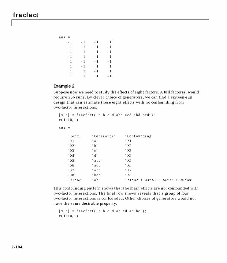
fracfact
2-104
ans = -1 -1 -1 1 -1 -1 1 -1 -1 1 -1 -1 -1 1 1 1 1 -1 -1 -1 1 -1 1 1 1 1 -1 1 1 1 1 -1
Example 2Suppose now we need to study the effects of eight factors. A full factorial wouldrequire 256 runs. By clever choice of generators, we can find a sixteen-rundesign that can estimate those eight effects with no confounding fromtwo-factor interactions.
[x,c] = fracfact('a b c d abc acd abd bcd');c(1:10,:)
ans =
'Term' 'Generator' 'Confounding' 'X1' 'a' 'X1' 'X2' 'b' 'X2' 'X3' 'c' 'X3' 'X4' 'd' 'X4' 'X5' 'abc' 'X5' 'X6' 'acd' 'X6' 'X7' 'abd' 'X7' 'X8' 'bcd' 'X8' 'X1*X2' 'ab' 'X1*X2 + X3*X5 + X4*X7 + X6*X8'
This confounding pattern shows that the main effects are not confounded withtwo-factor interactions. The final row shown reveals that a group of fourtwo-factor interactions is confounded. Other choices of generators would nothave the same desirable property.
[x,c] = fracfact('a b c d ab cd ad bc');c(1:10,:)

fracfact
2-105
ans =
'Term' 'Generator' 'Confounding' 'X1' 'a' 'X1 + X2*X5 + X4*X7' 'X2' 'b' 'X2 + X1*X5 + X3*X8' 'X3' 'c' 'X3 + X2*X8 + X4*X6' 'X4' 'd' 'X4 + X1*X7 + X3*X6' 'X5' 'ab' 'X5 + X1*X2' 'X6' 'cd' 'X6 + X3*X4' 'X7' 'ad' 'X7 + X1*X4' 'X8' 'bc' 'X8 + X2*X3' 'X1*X2' 'ab' 'X5 + X1*X2'
Here all the main effects are confounded with one or more two-factorinteractions.
References Box, G. A. F., W. G. Hunter, and J. S. Hunter (1978), Statistics forExperimenters, Wiley, New York.
See Also ff2n, fullfact, hadamard

friedman
2-106
2friedmanPurpose Friedman’s nonparametric two-way Analysis of Variance (ANOVA).
Syntax p = friedman(X,reps) p = friedman(X,reps,'displayopt') [p,table] = friedman(...)[p,table,stats] = friedman(...)
Description p = friedman(X,reps) performs the nonparametric Friedman’s test tocompare the means of the columns of X. Friedman’s test is similar to classicaltwo-way ANOVA, but it tests only for column effects after adjusting for possiblerow effects. It does not test for row effects or interaction effects. Friedman’s testis appropriate when columns represent treatments that are under study, androws represent nuisance effects (blocks) that need to be taken into account butare not of any interest.
The different columns represent changes in factor A. The different rowsrepresent changes in the blocking factor B. If there is more than oneobservation for each combination of factors, input reps indicates the number ofreplicates in each “cell,” which must be constant.
The matrix below illustrates the format for a set-up where column factor A hasthree levels, row factor B has two levels, and there are two replicates (reps=2).The subscripts indicate row, column, and replicate, respectively.
Friedman’s test assumes a model of the form
where is an overall location parameter, represents the column effect,represents the row effect, and represents the error. This test ranks thedata within each level of B, and tests for a difference across levels of A. The pthat friedman returns is the p-value for the null hypothesis that . If thep-value is near zero, this casts doubt on the null hypothesis. A sufficiently
x111 x121 x131
x112 x122 x132
x211 x221 x231
x212 x222 x232
xijk µ αi βj εijk+ + +=
µ αi βjεijk
αi 0=

friedman
2-107
small p-value suggests that at least one column-sample mean is significantlydifferent than the other column-sample means; i.e., there is a main effect dueto factor A. The choice of a limit for the p-value to determine whether a resultis “statistically significant” is left to the researcher. It is common to declare aresult significant if the p-value is less than 0.05 or 0.01.
friedman also displays a figure showing an ANOVA table, which divides thevariability of the ranks into two or three parts:
• The variability due to the differences among the column means
• The variability due to the interaction between rows and columns (if reps isgreater than its default value of 1)
• The remaining variability not explained by any systematic source
The ANOVA table has six columns:
• The first shows the source of the variability.
• The second shows the Sum of Squares (SS) due to each source.
• The third shows the degrees of freedom (df) associated with each source.
• The fourth shows the Mean Squares (MS), which is the ratio SS/df.
• The fifth shows Friedman’s chi-square statistic.
• The sixth shows the p-value for the chi-square statistic.
p = friedman(X,reps,'displayopt') enables the ANOVA table displaywhen 'displayopt' is 'on' (default) and suppresses the display when'displayopt' is 'off'.
[p,table] = friedman(...) returns the ANOVA table (including column androw labels) in cell array table. (You can copy a text version of the ANOVA tableto the clipboard by selecting Copy Text from the Edit menu.
[p,table,stats] = friedman(...) returns a stats structure that you canuse to perform a follow-up multiple comparison test. The friedman testevaluates the hypothesis that the column effects are all the same against thealternative that they are not all the same. Sometimes it is preferable toperform a test to determine which pairs of column effects are significantlydifferent, and which are not. You can use the multcompare function to performsuch tests by supplying the stats structure as input.
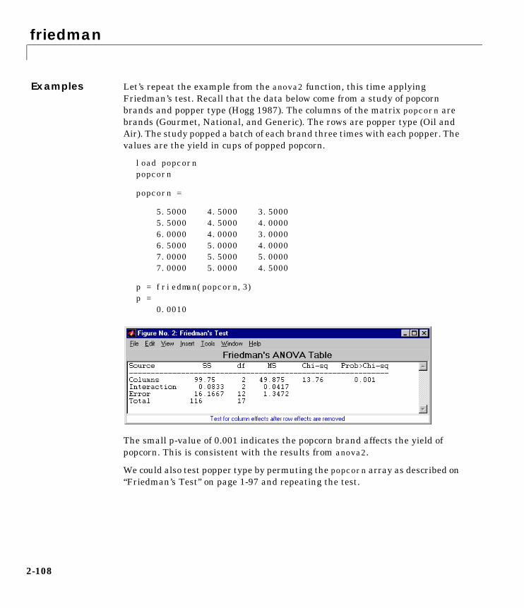
friedman
2-108
Examples Let’s repeat the example from the anova2 function, this time applyingFriedman’s test. Recall that the data below come from a study of popcornbrands and popper type (Hogg 1987). The columns of the matrix popcorn arebrands (Gourmet, National, and Generic). The rows are popper type (Oil andAir). The study popped a batch of each brand three times with each popper. Thevalues are the yield in cups of popped popcorn.
load popcornpopcorn
popcorn =
5.5000 4.5000 3.5000 5.5000 4.5000 4.0000 6.0000 4.0000 3.0000 6.5000 5.0000 4.0000 7.0000 5.5000 5.0000 7.0000 5.0000 4.5000
p = friedman(popcorn,3)p = 0.0010
The small p-value of 0.001 indicates the popcorn brand affects the yield ofpopcorn. This is consistent with the results from anova2.
We could also test popper type by permuting the popcorn array as described on“Friedman’s Test” on page 1-97 and repeating the test.

friedman
2-109
References Hogg, R. V. and J. Ledolter. Engineering Statistics. MacMillan PublishingCompany, 1987.
Hollander, M. and D. A. Wolfe. Nonparametric Statistical Methods. Wiley,1973.
See Also anova2, multcompare

frnd
2-110
2frndPurpose Random numbers from the F distribution.
Syntax R = frnd(V1,V2)R = frnd(V1,V2,m)R = frnd(V1,V2,m,n)
Description R = frnd(V1,V2) generates random numbers from the F distribution withnumerator degrees of freedom V1 and denominator degrees of freedom V2.Vector or matrix inputs for V1 and V2 must have the same size, which is alsothe size of R. A scalar input for V1 or V2 is expanded to a constant matrix withthe same dimensions as the other input.
R = frnd(V1,V2,m) generates random numbers from the F distribution withparameters V1 and V2, where m is a 1-by-2 vector that contains the row andcolumn dimensions of R.
R = frnd(V1,V2,m,n) generates random numbers from the F distributionwith parameters V1 and V2, where scalars m and n are the row and columndimensions of R.
Examples n1 = frnd(1:6,1:6)
n1 = 0.0022 0.3121 3.0528 0.3189 0.2715 0.9539
n2 = frnd(2,2,[2 3])
n2 = 0.3186 0.9727 3.0268 0.2052 148.5816 0.2191
n3 = frnd([1 2 3;4 5 6],1,2,3)
n3 = 0.6233 0.2322 31.5458 2.5848 0.2121 4.4955
See Also fcdf, finv, fpdf, fstat

fstat
2-111
2fstatPurpose Mean and variance for the F distribution.
Syntax [M,V] = fstat(V1,V2)
Description [M,V] = fstat(V1,V2) returns the mean and variance for the F distributionwith parameters specified by V1 and V2. Vector or matrix inputs for V1 and V2must have the same size, which is also the size of M and V. A scalar input for V1or V2 is expanded to a constant matrix with the same dimensions as the otherinput.
The mean of the F distribution for values of ν2 greater than 2 is
The variance of the F distribution for values of ν2 greater than 4 is
The mean of the F distribution is undefined if ν2 is less than 3. The variance isundefined for ν2 less than 5.
Examples fstat returns NaN when the mean and variance are undefined.
[m,v] = fstat(1:5,1:5)
m =NaN NaN 3.0000 2.0000 1.6667
v =NaN NaN NaN NaN 8.8889
See Also fcdf, finv, frnd, frnd
ν2ν2 2–------------
2ν22 ν1 ν2 2–+( )
ν1 ν2 2–( )2 ν2 4–( )--------------------------------------------------

fsurfht
2-112
2fsurfhtPurpose Interactive contour plot of a function.
Syntax fsurfht('fun',xlims,ylims)fsurfht('fun',xlims,ylims,p1,p2,p3,p4,p5)
Description fsurfht('fun',xlims,ylims) is an interactive contour plot of the functionspecified by the text variable fun. The x-axis limits are specified by xlims inthe form [xmin xmax], and the y-axis limits are specified by ylims in the form[ymin ymax].
fsurfht('fun',xlims,ylims,p1,p2,p3,p4,p5) allows for five optionalparameters that you can supply to the function fun.
The intersection of the vertical and horizontal reference lines on the plotdefines the current x-value and y-value. You can drag these reference lines andwatch the calculated z-values (at the top of the plot) update simultaneously.Alternatively, you can type the x-value and y-value into editable text fields onthe x-axis and y-axis.
Example Plot the Gaussian likelihood function for the gas.mat data.
load gas
Create a function containing the following commands, and name itgauslike.m.
function z = gauslike(mu,sigma,p1)n = length(p1);z = ones(size(mu));for i = 1:nz = z .* (normpdf(p1(i),mu,sigma));end
The gauslike function calls normpdf, treating the data sample as fixed and theparameters µ and σ as variables. Assume that the gas prices are normallydistributed, and plot the likelihood surface of the sample.
fsurfht('gauslike',[112 118],[3 5],price1)

fsurfht
2-113
The sample mean is the x-value at the maximum, but the sample standarddeviation is not the y-value at the maximum.
mumax = mean(price1)
mumax =
115.1500
sigmamax = std(price1)*sqrt(19/20)
sigmamax =
3.7719
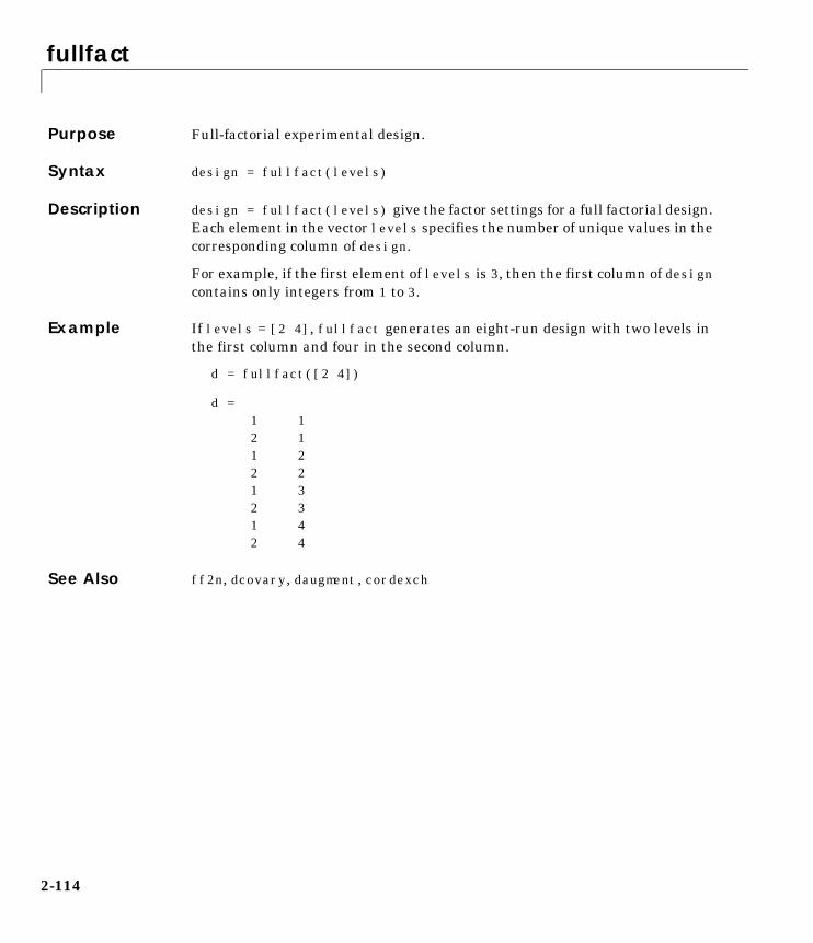
fullfact
2-114
2fullfactPurpose Full-factorial experimental design.
Syntax design = fullfact(levels)
Description design = fullfact(levels) give the factor settings for a full factorial design.Each element in the vector levels specifies the number of unique values in thecorresponding column of design.
For example, if the first element of levels is 3, then the first column of designcontains only integers from 1 to 3.
Example If levels = [2 4], fullfact generates an eight-run design with two levels inthe first column and four in the second column.
d = fullfact([2 4])
d = 1 1 2 1 1 2 2 2 1 3 2 3 1 4 2 4
See Also ff2n, dcovary, daugment, cordexch

gamcdf
2-115
2gamcdfPurpose Gamma cumulative distribution function (cdf).
Syntax P = gamcdf(X,A,B)
Description gamcdf(X,A,B) computes the gamma cdf at each of the values in X using thecorresponding parameters in A and B. Vector or matrix inputs for X, A, and Bmust all be the same size. A scalar input is expanded to a constant matrix withthe same dimensions as the other inputs. The parameters in A and B must bepositive.
The gamma cdf is
The result, p, is the probability that a single observation from a gammadistribution with parameters a and b will fall in the interval [0 x].
gammainc is the gamma distribution with b fixed at 1.
Examples a = 1:6;b = 5:10;prob = gamcdf(a.∗b,a,b)
prob =
0.6321 0.5940 0.5768 0.5665 0.5595 0.5543
The mean of the gamma distribution is the product of the parameters, ab. Inthis example, the mean approaches the median as it increases (i.e., thedistribution becomes more symmetric).
See Also cdf, gamfit, gaminv, gamlike, gampdf, gamrnd, gamstat
p F x a b,( ) 1
baΓ a( )------------------ ta 1– e
tb---–
td0
x
�= =
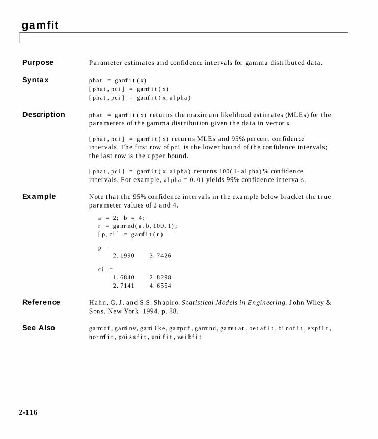
gamfit
2-116
2gamfitPurpose Parameter estimates and confidence intervals for gamma distributed data.
Syntax phat = gamfit(x)[phat,pci] = gamfit(x)[phat,pci] = gamfit(x,alpha)
Description phat = gamfit(x) returns the maximum likelihood estimates (MLEs) for theparameters of the gamma distribution given the data in vector x.
[phat,pci] = gamfit(x) returns MLEs and 95% percent confidenceintervals. The first row of pci is the lower bound of the confidence intervals;the last row is the upper bound.
[phat,pci] = gamfit(x,alpha) returns 100(1-alpha)% confidenceintervals. For example, alpha = 0.01 yields 99% confidence intervals.
Example Note that the 95% confidence intervals in the example below bracket the trueparameter values of 2 and 4.
a = 2; b = 4;r = gamrnd(a,b,100,1);[p,ci] = gamfit(r)
p = 2.1990 3.7426
ci = 1.6840 2.8298 2.7141 4.6554
Reference Hahn, G. J. and S.S. Shapiro. Statistical Models in Engineering. John Wiley &Sons, New York. 1994. p. 88.
See Also gamcdf, gaminv, gamlike, gampdf, gamrnd, gamstat, betafit, binofit, expfit,normfit, poissfit, unifit, weibfit

gaminv
2-117
2gaminvPurpose Inverse of the gamma cumulative distribution function (cdf).
Syntax X = gaminv(P,A,B)
Description X = gaminv(P,A,B) computes the inverse of the gamma cdf with parameters Aand B for the corresponding probabilities in P. Vector or matrix inputs for P, A,and B must all be the same size. A scalar input is expanded to a constant matrixwith the same dimensions as the other inputs. The parameters in A and B mustall be positive, and the values in P must lie on the interval [0 1].
The gamma inverse function in terms of the gamma cdf is
where
Algorithm There is no known analytical solution to the integral equation above. gaminvuses an iterative approach (Newton’s method) to converge on the solution.
Examples This example shows the relationship between the gamma cdf and its inversefunction.
a = 1:5;b = 6:10;x = gaminv(gamcdf(1:5,a,b),a,b)
x = 1.0000 2.0000 3.0000 4.0000 5.0000
See Also gamcdf, gamfit, gamlike, gampdf, gamrnd, gamstat, icdf
x F 1– p a b,( ) x:F x a b,( ) p={ }= =
p F x a b,( ) 1
baΓ a( )------------------ ta 1– e
tb---–
td0
x
�= =

gamlike
2-118
2gamlikePurpose Negative gamma log-likelihood function.
Syntax logL = gamlike(params,data)[logL,avar] = gamlike(params,data)
Description logL = gamlike(params,data) returns the negative of the gammalog-likelihood function for the parameters, params, given data. The length ofoutput vector logL is the length of vector data.
[logL,avar] = gamlike(params,data) also returns avar, which is theasymptotic variance-covariance matrix of the parameter estimates when thevalues in params are the maximum likelihood estimates. avar is the inverse ofFisher's information matrix. The diagonal elements of avar are the asymptoticvariances of their respective parameters.
gamlike is a utility function for maximum likelihood estimation of the gammadistribution. Since gamlike returns the negative gamma log-likelihoodfunction, minimizing gamlike using fminsearch is the same as maximizing thelikelihood.
Example This example continues the example for gamfit.
a = 2; b = 3;r = gamrnd(a,b,100,1);[logL,info] = gamlike([2.1990 2.8069],r)
logL =
267.5585
info =
0.0690 -0.0790 -0.0790 0.1220
See Also betalike, gamcdf, gamfit, gaminv, gampdf, gamrnd, gamstat, mle, weiblike

gampdf
2-119
2gampdfPurpose Gamma probability density function (pdf).
Syntax Y = gampdf(X,A,B)
Description gampdf(X,A,B) computes the gamma pdf at each of the values in X using thecorresponding parameters in A and B. Vector or matrix inputs for X, A, and Bmust all be the same size. A scalar input is expanded to a constant matrix withthe same dimensions as the other inputs. The parameters in A and B must allbe positive, and the values in X must lie on the interval [0 ∞).
The gamma pdf is
The gamma probability density function is useful in reliability models oflifetimes. The gamma distribution is more flexible than the exponentialdistribution in that the probability of a product surviving an additional periodmay depend on its current age. The exponential and χ2 functions are specialcases of the gamma function.
Examples The exponential distribution is a special case of the gamma distribution.
mu = 1:5;y = gampdf(1,1,mu)
y = 0.3679 0.3033 0.2388 0.1947 0.1637
y1 = exppdf(1,mu)
y1 = 0.3679 0.3033 0.2388 0.1947 0.1637
See Also gamcdf, gamfit, gaminv, gamlike, gamrnd, gamstat, pdf
y f x a b,( ) 1
baΓ a( )------------------xa 1– e
xb---–
= =

gamrnd
2-120
2gamrndPurpose Random numbers from the gamma distribution.
Syntax R = gamrnd(A,B)R = gamrnd(A,B,m)R = gamrnd(A,B,m,n)
Description R = gamrnd(A,B) generates gamma random numbers with parameters Aand B. Vector or matrix inputs for A and B must have the same size, which isalso the size of R. A scalar input for A or B is expanded to a constant matrix withthe same dimensions as the other input.
R = gamrnd(A,B,m) generates gamma random numbers with parameters Aand B, where m is a 1-by-2 vector that contains the row and column dimensionsof R.
R = gamrnd(A,B,m,n) generates gamma random numbers with parameters Aand B, where scalars m and n are the row and column dimensions of R.
Examples n1 = gamrnd(1:5,6:10)
n1 = 9.1132 12.8431 24.8025 38.5960 106.4164
n2 = gamrnd(5,10,[1 5])
n2 = 30.9486 33.5667 33.6837 55.2014 46.8265
n3 = gamrnd(2:6,3,1,5)
n3 = 12.8715 11.3068 3.0982 15.6012 21.6739
See Also gamcdf, gamfit, gaminv, gamlike, gampdf, gamstat
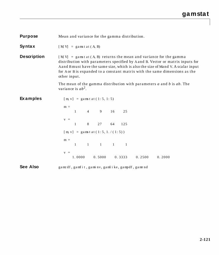
gamstat
2-121
2gamstatPurpose Mean and variance for the gamma distribution.
Syntax [M,V] = gamstat(A,B)
Description [M,V] = gamstat(A,B) returns the mean and variance for the gammadistribution with parameters specified by A and B. Vector or matrix inputs forA and Bmust have the same size, which is also the size of M and V. A scalar inputfor A or B is expanded to a constant matrix with the same dimensions as theother input.
The mean of the gamma distribution with parameters a and b is ab. Thevariance is ab2.
Examples [m,v] = gamstat(1:5,1:5)
m = 1 4 9 16 25
v = 1 8 27 64 125
[m,v] = gamstat(1:5,1./(1:5))
m = 1 1 1 1 1
v = 1.0000 0.5000 0.3333 0.2500 0.2000
See Also gamcdf, gamfit, gaminv, gamlike, gampdf, gamrnd

geocdf
2-122
2geocdfPurpose Geometric cumulative distribution function (cdf).
Syntax Y = geocdf(X,P)
Description geocdf(X,P) computes the geometric cdf at each of the values in X using thecorresponding probabilities in P. Vector or matrix inputs for X and P must bethe same size. A scalar input is expanded to a constant matrix with the samedimensions as the other input. The parameters in P must lie on the interval[0 1].
The geometric cdf is
where .
The result, y, is the probability of observing up to x trials before a success, whenthe probability of success in any given trial is p.
Examples Suppose you toss a fair coin repeatedly. If the coin lands face up (heads), thatis a success. What is the probability of observing three or fewer tails beforegetting a heads?
p = geocdf(3,0.5)
p = 0.9375
See Also cdf, geoinv, geopdf, geornd, geostat
y F x p( ) pqi
i 0=
floor x( )
�= =
q 1 p–=

geoinv
2-123
2geoinvPurpose Inverse of the geometric cumulative distribution function (cdf).
Syntax X = geoinv(Y,P)
Description X = geoinv(Y,P) returns the smallest positive integer X such that thegeometric cdf evaluated at X is equal to or exceeds Y. You can think of Y as theprobability of observing X successes in a row in independent trials where P isthe probability of success in each trial.
Vector or matrix inputs for P and Y must have the same size, which is also thesize of X. A scalar input for P and Y is expanded to a constant matrix with thesame dimensions as the other input. The values in P and Y must lie on theinterval [0 1].
Examples The probability of correctly guessing the result of 10 coin tosses in a row is lessthan 0.001 (unless the coin is not fair).
psychic = geoinv(0.999,0.5)
psychic =
9
The example below shows the inverse method for generating random numbersfrom the geometric distribution.
rndgeo = geoinv(rand(2,5),0.5)
rndgeo =
0 1 3 1 0 0 1 0 2 0
See Also geocdf, geopdf, geornd, geostat, icdf

geomean
2-124
2geomeanPurpose Geometric mean of a sample.
Syntax m = geomean(X)
Description geomean calculates the geometric mean of a sample. For vectors, geomean(x) isthe geometric mean of the elements in x. For matrices, geomean(X) is a rowvector containing the geometric means of each column.
The geometric mean is
Examples The sample average is greater than or equal to the geometric mean.
x = exprnd(1,10,6);geometric = geomean(x)
geometric =
0.7466 0.6061 0.6038 0.2569 0.7539 0.3478
average = mean(x)
average =
1.3509 1.1583 0.9741 0.5319 1.0088 0.8122
See Also mean, median, harmmean, trimmean
m xi
i 1=
n
∏
1n---
=
geopdf
2-125
2geopdfPurpose Geometric probability density function (pdf).
Syntax Y = geopdf(X,P)
Description geocdf(X,P) computes the geometric pdf at each of the values in X using thecorresponding probabilities in P. Vector or matrix inputs for X and P must bethe same size. A scalar input is expanded to a constant matrix with the samedimensions as the other input. The parameters in P must lie on the interval[0 1].
The geometric pdf is
where .
Examples Suppose you toss a fair coin repeatedly. If the coin lands face up (heads), thatis a success. What is the probability of observing exactly three tails beforegetting a heads?
p = geopdf(3,0.5)
p = 0.0625
See Also geocdf, geoinv, geornd, geostat, pdf
y f x p( ) pqxI 0 1 K, ,( ) x( )= =
q 1 p–=

geornd
2-126
2georndPurpose Random numbers from the geometric distribution.
Syntax R = geornd(P)R = geornd(P,m)R = geornd(P,m,n)
Description The geometric distribution is useful when you want to model the number ofsuccessive failures preceding a success, where the probability of success in anygiven trial is the constant P.
R = geornd(P) generates geometric random numbers with probabilityparameter P. The size of R is the size of P.
R = geornd(P,m) generates geometric random numbers with probabilityparameter P, where m is a 1-by-2 vector that contains the row and columndimensions of R.
R = geornd(P,m,n) generates geometric random numbers with probabilityparameter P, where scalars m and n are the row and column dimensions of R.
The parameters in P must lie on the interval [0 1].
Examples r1 = geornd(1 ./ 2.^(1:6))
r1 = 2 10 2 5 2 60
r2 = geornd(0.01,[1 5])
r2 = 65 18 334 291 63
r3 = geornd(0.5,1,6)
r3 = 0 7 1 3 1 0
See Also geocdf, geoinv, geopdf, geostat
geostat
2-127
2geostatPurpose Mean and variance for the geometric distribution.
Syntax [M,V] = geostat(P)
Description [M,V] = geostat(P) returns the mean and variance for the geometricdistribution with parameters specified by P.
The mean of the geometric distribution with parameter p is q/p, where q = 1-p.The variance is q/p2.
Examples [m,v] = geostat(1./(1:6))
m =0 1.0000 2.0000 3.0000 4.0000 5.0000
v =0 2.0000 6.0000 12.0000 20.0000 30.0000
See Also geocdf, geoinv, geopdf, geornd

gline
2-128
2glinePurpose Interactively draw a line in a figure.
Syntax gline(fig)h = gline(fig)gline
Description gline(fig) allows you to draw a line segment in the figure fig by clicking thepointer at the two end-points. A rubber band line tracks the pointer movement.
h = gline(fig) returns the handle to the line in h.
gline with no input arguments draws in the current figure.
See Also refline, gname

glmdemo
2-129
2glmdemoPurpose Demo of generalized linear models.
Syntax glmdemo
Description glmdemo begins a slide show demonstration of generalized linear models. Theslides indicate when generalized linear models are useful, how to fitgeneralized linear models using the glmfit function, and how to makepredictions using the glmval function.
See Also glmfit, glmval

glmfit
2-130
2glmfitPurpose Generalized linear model fitting.
Syntax b = glmfit(X,Y,'distr')b = glmfit(X,Y,'distr','link','estdisp',offset,pwts,'const')[b,dev,stats] = glmfit(...)
Description b = glmfit(x,y,'distr') fits the generalized linear model for response Y,predictor variable matrix X, and distribution 'distr'. The followingdistributions are available: 'binomial', 'gamma', 'inverse gaussian','lognormal', 'normal' (the default), and 'poisson'. In most cases Y is avector of response measurements, but for the binomial distribution Y is atwo-column array having the measured number of counts in the first columnand the number of trials (the binomial N parameter) in the second column. X isa matrix having the same number of rows as Y and containing the values of thepredictor variables for each observation. The output b is a vector of coefficientestimates. This syntax uses the canonical link (see below) to relate thedistribution parameter to the predictors.
b = glmfit(x,y,'distr','link','estdisp',offset,pwts,'const')provides additional control over the fit. The 'link' argument specifies therelationship between the distribution parameter (µ) and the fitted linearcombination of predictor variables (xb). In most cases 'link' is one of thefollowing:
'link' Meaning Default (Canonical) Link
'identity' µ = xb 'normal'
'log' log(µ) = xb 'poisson'
'logit' log(µ / (1-µ)) = xb 'binomial'
'probit' norminv(µ) = xb
'comploglog' log(-log(1-µ)) = xb
'logloglink' log(-log(µ)) = xb
'reciprocal' 1/µ = xb 'gamma'
p (a number) µp = xb 'inverse gaussian' (with p=-2)

glmfit
2-131
Alternatively, you can write functions to define your own custom link. Youspecify the link argument as a three-element cell array containing functionsthat define the link function, its derivative, and its inverse. For example,suppose you want to define a reciprocal square root link using inline functions.You could define the variable mylinks to use as your 'link' argument bywriting:
FL = inline('x.^-.5')FD = inline('-.5*x.^-1.5')FI = inline('x.^-2')mylinks = {FL FI FD}
Alternatively, you could define functions named FL, FD, and FI in their ownM-files, and then specify mylinks in the form
mylinks = {@FL @FD @FI}
The 'estdisp' argument can be 'on' to estimate a dispersion parameter forthe binomial or Poisson distribution, or 'off' (the default) to use thetheoretical value of 1.0 for those distributions. The glmfit function alwaysestimates dispersion parameters for other distributions.
The offset and pwts parameters can be vectors of the same length as Y, or canbe omitted (or specified as an empty vector). The offset vector is a specialpredictor variable whose coefficient is known to be 1.0. As an example, supposethat you are modeling the number of defects on various surfaces, and you wantto construct a model in which the expected number of defects is proportional tothe surface area. You might use the number of defects as your response, alongwith the Poisson distribution, the log link function, and the log surface area asan offset.
The pwts argument is a vector of prior weights. As an example, if the responsevalue Y(i) is the average of f(i) measurements, you could use f as a vector ofprior weights.
The 'const' argument can be 'on' (the default) to estimate a constant term,or 'off' to omit the constant term. If you want the constant term, use thisargument rather than specifying a column of ones in the X matrix.
[b,dev,stats] = glmfit(...) returns the additional outputs dev and stats.dev is the deviance at the solution vector. The deviance is a generalization ofthe residual sum of squares. It is possible to perform an analysis of deviance to

glmfit
2-132
compare several models, each a subset of the other, and to test whether themodel with more terms is significantly better than the model with fewer terms.
stats is a structure with the following fields:
• stats.dfe = degrees of freedom for error
• stats.s = theoretical or estimated dispersion parameter
• stats.sfit = estimated dispersion parameter
• stats.estdisp = 1 if dispersion is estimated, 0 if fixed
• stats.beta = vector of coefficient estimates (same as b)
• stats.se = vector of standard errors of the coefficient estimates b
• stats.coeffcorr = correlation matrix for b
• stats.t = t statistics for b
• stats.p = p-values for b
• stats.resid = vector of residuals
• stats.residp = vector of Pearson residuals
• stats.residd = vector of deviance residuals
• stats.resida = vector of Anscombe residuals
If you estimate a dispersion parameter for the binomial or Poisson distribution,then stats.s is set equal to stats.sfit. Also, the elements of stats.se differby the factor stats.s from their theoretical values.
Example We have data on cars weighing between 2100 and 4300 pounds. For each carweight we have the total number of cars of that weight, and the number thatcan be considered to get “poor mileage” according to some test. For example, 8out of 21 cars weighing 3100 pounds get poor mileage according to ameasurement of the miles they can travel on a gallon of gasoline.
w = (2100:200:4300)';poor = [1 2 0 3 8 8 14 17 19 15 17 21]';total = [48 42 31 34 31 21 23 23 21 16 17 21]';
We can compare several fits to these data. First, let’s try fitting logit and probitmodels:
[bl,dl,sl] = glmfit(w,[poor total],'binomial');[bp,dp,sp] = glmfit(w,[poor total],'binomial','probit');

glmfit
2-133
dldl = 6.4842
dpdp = 7.5693
The deviance for the logit model is smaller than for the probit model. Althoughthis is not a formal test, it leads us to prefer the logit model.
We can do a formal test comparing two logit models. We already fit one modelusing w as a linear predictor. Let’s fit another logit model using both linear andsquared terms in w. If there is no true effect for the squared term, the differencein their deviances should be small compared with a chi-square distributionhaving one degree of freedom.
[b2,d2,s2] = glmfit([w w.^2],[poor total],'binomial')
dl-d2
ans = 0.7027
chi2cdf(dl-d2,1)
ans = 0.5981
A difference of 0.7072 is not at all unusual for a chi-square distribution withone degree of freedom, so the quadratic model does not give a significantlybetter fit than the simpler linear model.
The following are the coefficient estimates, their standard errors, t-statistics,and p-values for the linear model:
[b sl.se sl.t sl.p]
ans =
-13.3801 1.3940 -9.5986 0.0000 0.0042 0.0004 9.4474 0.0000

glmfit
2-134
This shows that we cannot simplify the model any further. Both the interceptand slope coefficients are significantly different from 0, as indicated byp-values that are 0.0000 to four decimal places.
See Also glmval, glmdemo, nlinfit, regress, regstats
References Dobson, A. J. An Introduction to Generalized Linear Models. 1990, CRC Press.
MuCullagh, P. and J. A. Nelder. Generalized Linear Models. 2nd edition, 1990,Chapman and Hall.

glmval
2-135
2glmvalPurpose Compute predictions for generalized linear model.
Syntax yfit = glmval(b,X,'link')[yfit,dlo,dhi] = glmval(b,X,'link',stats,clev)[yfit,dlo,dhi] = glmval(b,X,'link',stats,clev,N,offset,'const')
Description yfit = glmval(b,X,'link') computes the predicted distribution parametersfor observations with predictor values X using the coefficient vector b and linkfunction 'link'. Typically, b is a vector of coefficient estimates computed bythe glmfit function. The value of 'link' must be the same as that used inglmfit. The result yfit is the value of the inverse of the link function at thelinear combination X*b.
[yfit,dlo,dhi] = glmval(b,X,'link',stats,clev) returns confidencebounds for the predicted values when you supply the stats structure returnedfrom glmfit, and optionally specify a confidence level as the clev argument.(The default confidence level is 0.95 for 95% confidence.) The interval[yfit-dlo, yfit+dhi] is a confidence bound for the true parameter value atthe specified X values.
[yhat,dlo,dhi] = glmval(beta,X,'link',stats,clev,N,offset,'const')specifies three additional arguments that may be needed if you used certainarguments to glmfit. If you fit a binomial distribution using glmfit, specify Nas the value of the binomial N parameter for the predictions. If you included anoffset variable, specify offset as the new value of this variable. Use the same'const' value ('on' or 'off') that you used with glmfit.
Example Let's model the number of cars with poor gasoline mileage using the binomialdistribution. First we use the binomial distribution with the default logit linkto model the probability of having poor mileage as a function of the weight andsquared weight of the cars. Then we compute a vector wnew of new car weightsat which we want to make predictions. Next we compute the expected numberof cars, out of a total of 30 cars of each weight, that would have poor mileage.Finally we graph the predicted values and 95% confidence bounds as a functionof weight.
w = [2100 2300 2500 2700 2900 3100 3300 3500 3700 3900 4100 4300]';poor = [1 2 0 3 8 8 14 17 19 15 17 21]';total = [48 42 31 34 31 21 23 23 21 16 17 21]';

glmval
2-136
[b2,d2,s2] = glmfit([w w.^2],[poor total],'binomial')wnew = (3000:100:4000)';[yfit,dlo,dhi] = glmval(b2,[wnew wnew.^2],'logit',s2,0.95,30)errorbar(wnew,yfit,dlo,dhi);
See Also glmfit, glmdemo
2800 3000 3200 3400 3600 3800 4000 42005
10
15
20
25
30

gname
2-137
2gnamePurpose Label plotted points with their case names or case number.
Syntax gname('cases')gnameh = gname('cases',line_handle)
Description gname('cases') displays a figure window, displays cross-hairs, and waits fora mouse button or keyboard key to be pressed. Position the cross-hair with themouse and click once near each point to label that point. Input 'cases' is astring matrix with each row the case name of a data point. You can also clickand drag a selection rectangle to label all points within the rectangle. Whenyou are done, press the Enter or Escape key.
gname with no arguments labels each case with its case number.
h = gname('cases',line_handle) returns a vector of handles to the textobjects on the plot. Use the scalar line_handle to identify the correct line ifthere is more than one line object on the plot.
You can use gname to label plots created by the plot, scatter, gscatter,plotmatrix, and gplotmatrix functions.
Example Let’s use the city ratings data sets to find out which cities are the best andworst for education and the arts. We create a graph, call the gname function,and click on the points at the extreme left and at the top.
load citieseducation = ratings(:,6);arts = ratings(:,7);plot(education,arts,'+')gname(names)

gname
2-138
See Also gplotmatrix, gscatter, gtext, plot, plotmatrix, scatter
1500 2000 2500 3000 3500 40000
1
2
3
4
5
6x 10⁴
Pascagoula, MS
New York, NY

gplotmatrix
2-139
2gplotmatrixPurpose Plot matrix of scatter plots by group.
Syntax gplotmatrix(x,y,g)gplotmatrix(x,y,g,'clr','sym',siz)gplotmatrix(x,y,g,'clr','sym',siz,'doleg')gplotmatrix(x,y,g,'clr','sym',siz,'doleg','dispopt')gplotmatrix(x,y,g,'clr','sym',siz,'doleg','dispopt','xnam','ynam')[h,ax,bigax] = gplotmatrix(...)
Description gplotmatrix(x,y,g) creates a matrix of scatter plots. Each individual set ofaxes in the resulting figure contains a scatter plot of a column of x against acolumn of y. All plots are grouped by the grouping variable g.
x and y are matrices with the same number of rows. If x has p columns and yhas q columns, the figure contains a p-by-q matrix of scatter plots. If you omity or specify it as the empty matrix, [], gplotmatrix creates a square matrix ofscatter plots of columns of x against each other.
g is a grouping variable that can be a vector, string array, or cell array ofstrings. g must have the same number of rows as x and y. Points with the samevalue of g are placed in the same group, and appear on the graph with the samemarker and color. Alternatively, g can be a cell array containing severalgrouping variables (such as {G1 G2 G3}); in that case, observations are in thesame group if they have common values of all grouping variables.
gplotmatrix(x,y,g,'clr','sym',siz) specifies the color, marker type, andsize for each group. clr is a string array of colors recognized by the plotfunction. The default is 'clr' = 'bgrcmyk'. 'sym' is a string array of symbolsrecognized by the plot command, with the default value '.'. siz is a vector ofsizes, with the default determined by the 'defaultlinemarkersize' property.If you do not specify enough values for all groups, gplotmatrix cycles throughthe specified values as needed.
gplotmatrix(x,y,g,'clr','sym',siz,'doleg') controls whether a legend isdisplayed on the graph ('doleg' = 'on', the default) or not ('doleg' = 'off').

gplotmatrix
2-140
gplotmatrix(x,y,g,'clr','sym',siz,'doleg','dispopt') controls whatappears along the diagonal of a plot matrix of x versus x. Allowable values are'none' to leave the diagonals blank, 'hist' (the default) to plot histograms, or'variable' to write the variable names.
gplotmatrix(x,y,g,'clr','sym',siz,'doleg','dispopt','xnam','ynam')specifies the names of the columns in the x and y arrays. These names are usedto label the x- and y-axes. 'xnam' and 'ynam' must be character arrays withone row for each column of x and y, respectively.
[h,ax,bigax] = gplotmatrix(...) returns three arrays of handles. h is anarray of handles to the lines on the graphs. ax is a matrix of handles to the axesof the individual plots. bigax is a handle to big (invisible) axes framing theentire plot matrix. These are left as the current axes, so a subsequent title,xlabel, or ylabel command will produce labels that are centered with respectto the entire plot matrix.
Example Load the cities data. The ratings array has ratings of the cities in ninecategories (category names are in the array categories). group is a code whosevalue is 2 for the largest cities. We can make scatter plots of the first threecategories against the other four, grouped by the city size code.
load discrimgplotmatrix(ratings(:,1:3),ratings(:,4:7),group)
The output figure (not shown) has an array of graphs with each city grouprepresented by a different color. The graphs are a little easier to read if wespecify colors and plotting symbols, label the axes with the rating categories,and move the legend off the graphs.
gplotmatrix(ratings(:,1:3),ratings(:,4:7),group,...'br','.o',[],'on','',categories(1:3,:),...categories(4:7,:))
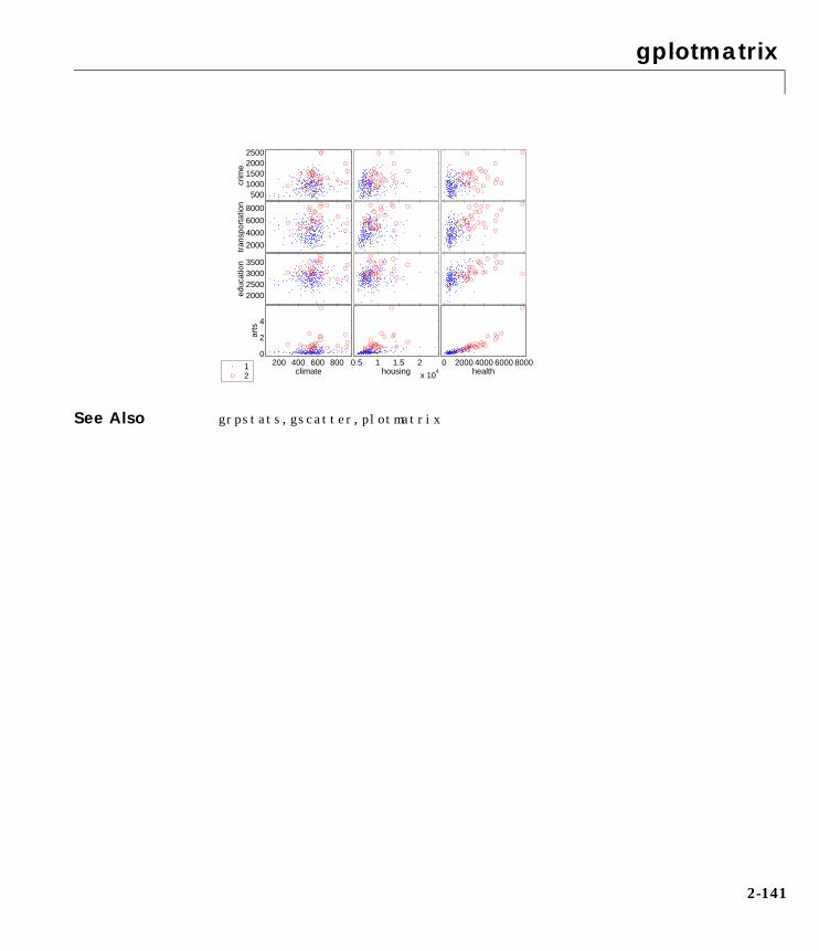
gplotmatrix
2-141
See Also grpstats, gscatter, plotmatrix
0 2000 4000 6000 8000health
0.5 1 1.5 2
x 104housing
200 400 600 8000
2
4
x 104
climate
arts
2000250030003500
educ
atio
n2000
4000
6000
8000
tran
spor
tatio
n
5001000150020002500
crim
e
12

grpstats
2-142
2grpstatsPurpose Summary statistics by group.
Syntax means = grpstats(X,group)[means,sem,counts,name] = grpstats(X,group)grpstats(x,group,alpha)
Description means = grpstats(X,group) returns the means of each column of X by group,where X is a matrix of observations. group is an array that defines the groupingsuch that two elements of X are in the same group if their corresponding groupvalues are the same. The grouping variable group can be a vector, string array,or cell array of strings. It can also be a cell array containing several groupingvariables (such as {G1 G2 G3}); in that case observations are in the same groupif they have common values of all grouping variables.
[means,sem,counts,name] = grpstats(x,group,alpha) supplies thestandard error of the mean in sem, the number of elements in each group incounts, and the name of each group in name. name is useful to identify and labelthe groups when the input group values are not simple group numbers.
grpstats(x,group,alpha) plots 100(1-alpha)% confidence intervals aroundeach mean.
Example We assign 100 observations to one of four groups. For each observation wemeasure five quantities with true means from 1 to 5. grpstats allows us tocompute the means for each group.
group = unidrnd(4,100,1);true_mean = 1:5;true_mean = true_mean(ones(100,1),:);x = normrnd(true_mean,1);means = grpstats(x,group)
means =
0.7947 2.0908 2.8969 3.6749 4.6555 0.9377 1.7600 3.0285 3.9484 4.8169 1.0549 2.0255 2.8793 4.0799 5.3740 0.7107 1.9264 2.8232 3.8815 4.9689
See Also tabulate, crosstab
gscatter
2-143
2gscatterPurpose Scatter plot by group.
Syntax gscatter(x,y,g)gscatter(x,y,g,'clr','sym',siz)gscatter(x,y,g,'clr','sym',siz,'doleg')gscatter(x,y,g,'clr','sym',siz,'doleg','xnam','ynam')h = gscatter(...)
Description gscatter(x,y,g) creates a scatter plot of x and y, grouped by g, where x and yare vectors with the same size and g can be a vector, string array, or cell arrayof strings. Points with the same value of g are placed in the same group, andappear on the graph with the same marker and color. Alternatively, g can be acell array containing several grouping variables (such as {G1 G2 G3}); in thatcase, observations are in the same group if they have common values of allgrouping variables.
gscatter(x,y,g,'clr','sym',siz) specifies the color, marker type, and sizefor each group. 'clr' is a string array of colors recognized by the plot function.The default is 'clr' = 'bgrcmyk'. 'sym' is a string array of symbols recognizedby the plot command, with the default value '.'. siz is a vector of sizes, withthe default determined by the 'defaultlinemarkersize' property. If you donot specify enough values for all groups, gscatter cycles through the specifiedvalues as needed.
gscatter(x,y,g,'clr','sym',siz,'doleg') controls whether a legend isdisplayed on the graph ('doleg' = 'on', the default) or not ('doleg' = 'off').
gscatter(x,y,g,'clr','sym',siz,'doleg','xnam','ynam') specifies thename to use for the x-axis and y-axis labels. If the x and y inputs are simplevariable names and xnam and ynam are omitted, gscatter labels the axes withthe variable names.
h = gscatter(...) returns an array of handles to the lines on the graph.
Example Load the cities data and look at the relationship between the ratings forclimate (first column) and housing (second column) grouped by city size. We’llalso specify the colors and plotting symbols.

gscatter
2-144
load discrimgscatter(ratings(:,1),ratings(:,2),group,'br','xo')
See Also gplotmatrix, grpstats, scatter
100 200 300 400 500 600 700 800 900 10000.4
0.6
0.8
1
1.2
1.4
1.6
1.8
2
2.2
2.4x 10
4
12

harmmean
2-145
2harmmeanPurpose Harmonic mean of a sample of data.
Syntax m = harmmean(X)
Description m = harmmean(X) calculates the harmonic mean of a sample. For vectors,harmmean(x) is the harmonic mean of the elements in x. For matrices,harmmean(X) is a row vector containing the harmonic means of each column.
The harmonic mean is
Examples The sample average is greater than or equal to the harmonic mean.
x = exprnd(1,10,6);harmonic = harmmean(x)
harmonic =
0.3382 0.3200 0.3710 0.0540 0.4936 0.0907
average = mean(x)
average =
1.3509 1.1583 0.9741 0.5319 1.0088 0.8122
See Also mean, median, geomean, trimmean
m n
1xi----
i 1=
n
�
---------------=

hist
2-146
2histPurpose Plot histograms.
Syntax hist(y)hist(y,nb)hist(y,x)[n,x] = hist(y,...)
Description hist(y) draws a 10-bin histogram for the data in vector y. The bins are equallyspaced between the minimum and maximum values in y.
hist(y,nb) draws a histogram with nb bins.
hist(y,x) draws a histogram using the bins in the vector x.
[n,x] = hist(y,...) do not draw graphs, but return vectors n and xcontaining the frequency counts and the bin locations such that bar(x,n) plotsthe histogram. This is useful in situations where more control is needed overthe appearance of a graph, for example, to combine a histogram into a moreelaborate plot statement.
The hist function is a part of the standard MATLAB language.
Examples Generate bell-curve histograms from Gaussian data.
x = -2.9:0.1:2.9;y = normrnd(0,1,1000,1);hist(y,x)
-3 -2 -1 0 1 2 30
10
20
30
40
50
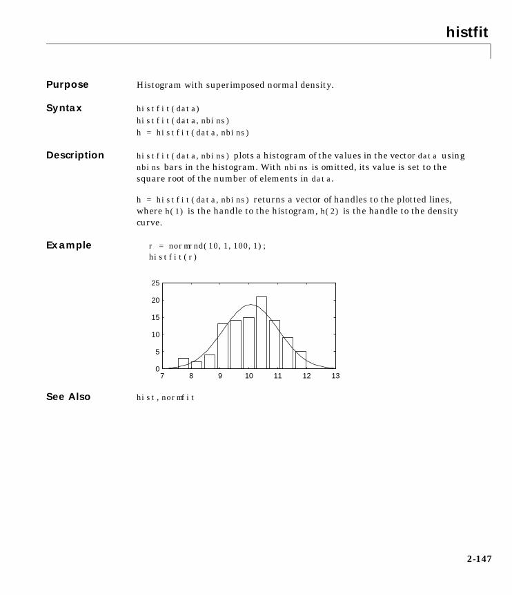
histfit
2-147
2histfitPurpose Histogram with superimposed normal density.
Syntax histfit(data)histfit(data,nbins)h = histfit(data,nbins)
Description histfit(data,nbins) plots a histogram of the values in the vector data usingnbins bars in the histogram. With nbins is omitted, its value is set to thesquare root of the number of elements in data.
h = histfit(data,nbins) returns a vector of handles to the plotted lines,where h(1) is the handle to the histogram, h(2) is the handle to the densitycurve.
Example r = normrnd(10,1,100,1);histfit(r)
See Also hist, normfit
7 8 9 10 11 12 130
5
10
15
20
25

hougen
2-148
2hougenPurpose Hougen-Watson model for reaction kinetics.
Syntax yhat = hougen(beta,x)
Description yhat = hougen(beta,x) returns the predicted values of the reaction rate,yhat, as a function of the vector of parameters, beta, and the matrix of data, X.beta must have 5 elements and X must have three columns.
hougen is a utility function for rsmdemo.
The model form is:
Reference Bates, D., and D. Watts. Nonlinear Regression Analysis and Its Applications.Wiley 1988. p. 271–272.
See Also rsmdemo
yβ1x2 x3 β5⁄–
1 β2x1 β3x2 β4x3+ + +-----------------------------------------------------------=

hygecdf
2-149
2hygecdfPurpose Hypergeometric cumulative distribution function (cdf).
Syntax P = hygecdf(X,M,K,N)
Description hygecdf(X,M,K,N) computes the hypergeometric cdf at each of the values in Xusing the corresponding parameters in M, K, and N. Vector or matrix inputs forX, M, K, and N must all have the same size. A scalar input is expanded to aconstant matrix with the same dimensions as the other inputs.
The hypergeometric cdf is
The result, p, is the probability of drawing up to x of a possible K items in Ndrawings without replacement from a group of M objects.
Examples Suppose you have a lot of 100 floppy disks and you know that 20 of them aredefective. What is the probability of drawing zero to two defective floppies ifyou select 10 at random?
p = hygecdf(2,100,20,10)
p = 0.6812
See Also cdf, hygeinv, hygepdf, hygernd, hygestat
p F x M K N, ,( )
Ki� �
� � M K–
N i–� �� �
MN� �
� �-------------------------------
i 0=
x
�= =
hygeinv
2-150
2hygeinvPurpose Inverse of the hypergeometric cumulative distribution function (cdf).
Syntax X = hygeinv(P,M,K,N)
Description hygeinv(P,M,K,N) returns the smallest integer X such that thehypergeometric cdf evaluated at X equals or exceeds P. You can think of P as theprobability of observing X defective items in N drawings without replacementfrom a group of M items where K are defective.
Examples Suppose you are the Quality Assurance manager for a floppy diskmanufacturer. The production line turns out floppy disks in batches of 1,000.You want to sample 50 disks from each batch to see if they have defects. Youwant to accept 99% of the batches if there are no more than 10 defective disksin the batch. What is the maximum number of defective disks should you allowin your sample of 50?
x = hygeinv(0.99,1000,10,50)
x = 3
What is the median number of defective floppy disks in samples of 50 disksfrom batches with 10 defective disks?
x = hygeinv(0.50,1000,10,50)
x = 0
See Also hygecdf, hygepdf, hygernd, hygestat, icdf
hygepdf
2-151
2hygepdfPurpose Hypergeometric probability density function (pdf).
Syntax Y = hygepdf(X,M,K,N)
Description Y = hygecdf(X,M,K,N) computes the hypergeometric pdf at each of the valuesin X using the corresponding parameters in M, K, and N. Vector or matrix inputsfor X, M, K, and N must all have the same size. A scalar input is expanded to aconstant matrix with the same dimensions as the other inputs.
The parameters in M, K, and N must all be positive integers, with N ≤ M. Thevalues in X must be less than or equal to all the parameter values.
The hypergeometric pdf is
The result, y, is the probability of drawing exactly x of a possible K items in ndrawings without replacement from a group of M objects.
Examples Suppose you have a lot of 100 floppy disks and you know that 20 of them aredefective. What is the probability of drawing 0 through 5 defective floppy disksif you select 10 at random?
p = hygepdf(0:5,100,20,10)
p = 0.0951 0.2679 0.3182 0.2092 0.0841 0.0215
See Also hygecdf, hygeinv, hygernd, hygestat, pdf
y f x M K N, ,( )
Kx� �
� � M K–
N x–� �� �
MN� �
� �-------------------------------= =

hygernd
2-152
2hygerndPurpose Random numbers from the hypergeometric distribution.
Syntax R = hygernd(M,K,N)R = hygernd(M,K,N,mm)R = hygernd(M,K,N,mm,nn)
Description R = hygernd(M,K,N) generates hypergeometric random numbers withparameters M, K, and N. Vector or matrix inputs for M, K, and N must have thesame size, which is also the size of R. A scalar input for M, K, or N is expanded toa constant matrix with the same dimensions as the other inputs.
R = hygernd(M,K,N,mm) generates hypergeometric random numbers withparameters M, K, and N, where mm is a 1-by-2 vector that contains the row andcolumn dimensions of R.
R = hygernd(M,K,N,mm,nn) generates hypergeometric random numbers withparameters M, K, and N, where scalars mm and nn are the row and columndimensions of R.
Examples numbers = hygernd(1000,40,50)
numbers =
1
See Also hygecdf, hygeinv, hygepdf, hygestat

hygestat
2-153
2hygestatPurpose Mean and variance for the hypergeometric distribution.
Syntax [MN,V] = hygestat(M,K,N)
Description [MN,V] = hygestat(M,K,N) returns the mean and variance for thehypergeometric distribution with parameters specified by M, K, and N. Vector ormatrix inputs for M, K, and N must have the same size, which is also the size ofMN and V. A scalar input for M, K, or N is expanded to a constant matrix with thesame dimensions as the other inputs.
The mean of the hypergeometric distribution with parameters M, K, and N isNK/M, and the variance is
Examples The hypergeometric distribution approaches the binomial distribution, wherep = K / M as M goes to infinity.
[m,v] = hygestat(10.^(1:4),10.^(0:3),9)
m = 0.9000 0.9000 0.9000 0.9000
v = 0.0900 0.7445 0.8035 0.8094
[m,v] = binostat(9,0.1)
m = 0.9000
v = 0.8100
See Also hygecdf, hygeinv, hygepdf, hygernd
N KM-----
M K–M
----------------M N–M 1–----------------

icdf
2-154
2icdfPurpose Inverse of a specified cumulative distribution function (icdf).
Syntax X = icdf('name',P,A1,A2,A3)
Description X = icdf('name',P,A1,A2,A3) returns a matrix of critical values, X, where'name' is a string containing the name of the distribution. P is a matrix ofprobabilities, and A, B, and C are matrices of distribution parameters.Depending on the distribution some of the parameters may not be necessary.
Vector or matrix inputs for P, A1, A2, and A3 must all have the same size. Ascalar input is expanded to a constant matrix with the same dimensions as theother inputs.
icdf is a utility routine allowing you to access all the inverse cdfs in theStatistics Toolbox using the name of the distribution as a parameter. See“Overview of the Distributions” on page 1-12 for the list of availabledistributions.
Examples x = icdf('Normal',0.1:0.2:0.9,0,1)
x = -1.2816 -0.5244 0 0.5244 1.2816
x = icdf('Poisson',0.1:0.2:0.9,1:5)
x = 1 1 3 5 8
See Also betainv, binoinv, cdf, chi2inv, expinv, finv, gaminv, geoinv, hygeinv,logninv, nbininv, ncfinv, nctinv, ncx2inv, norminv, pdf, poissinv, random,raylinv, tinv, unidinv, unifinv, weibinv

inconsistent
2-155
2inconsistentPurpose Calculate the inconsistency coefficient of a cluster tree.
Syntax Y = inconsistent(Z) Y = inconsistent(Z,d)
Description Y = inconsistent(Z) computes the inconsistency coefficient for each link ofthe hierarchical cluster tree Z, where Z is an (m-1)-by-3 matrix generated by thelinkage function. The inconsistency coefficient characterizes each link in acluster tree by comparing its length with the average length of other links atthe same level of the hierarchy. The higher the value of this coefficient, the lesssimilar the objects connected by the link.
Y = inconsistent(Z,d) computes the inconsistency coefficient for each linkin the hierarchical cluster tree Z to depth d, where d is an integer denoting thenumber of levels of the cluster tree that are included in the calculation. Bydefault, d=2.
The output, Y, is an (m-1)-by-4 matrix formatted as follows.
For each link, k, the inconsistency coefficient is calculated as:
For leaf nodes, nodes that have no further nodes under them, the inconsistencycoefficient is set to 0.
Column Description
1 Mean of the lengths of all the links included in the calculation.
2 Standard deviation of all the links included in the calculation.
3 Number of links included in the calculation.
4 Inconsistency coefficient.
Y k 4,( ) z k 3,( ) Y k 1,( )–( ) Y k 2,( )⁄=

inconsistent
2-156
Example rand('seed',12);X = rand(10,2);Y = pdist(X);Z = linkage(Y,'centroid');W = inconsistent(Z,3)
W =
0.0423 0 1.0000 0 0.1406 0 1.0000 0 0.1163 0.1047 2.0000 0.70710.2101 0 1.0000 00.2054 0.0886 3.0000 0.67920.1742 0.1762 3.0000 0.65680.2336 0.1317 4.0000 0.64080.3081 0.2109 5.0000 0.79890.4610 0.3728 4.0000 0.8004
See Also cluster, cophenet, clusterdata, dendrogram, linkage, pdist, squareform
iqr
2-157
2iqrPurpose Interquartile range (IQR) of a sample.
Syntax y = iqr(X)
Description y = iqr(X) computes the difference between the 75th and the 25th percentilesof the sample in X. The IQR is a robust estimate of the spread of the data, sincechanges in the upper and lower 25% of the data do not affect it.
If there are outliers in the data, then the IQR is more representative than thestandard deviation as an estimate of the spread of the body of the data. TheIQR is less efficient than the standard deviation as an estimate of the spreadwhen the data is all from the normal distribution.
Multiply the IQR by 0.7413 to estimate σ (the second parameter of the normaldistribution.)
Examples This Monte Carlo simulation shows the relative efficiency of the IQR to thesample standard deviation for normal data.
x = normrnd(0,1,100,100);s = std(x);s_IQR = 0.7413 ∗ iqr(x);efficiency = (norm(s - 1)./norm(s_IQR - 1)).^2
efficiency =
0.3297
See Also std, mad, range

jbtest
2-158
2jbtestPurpose Jarque-Bera test for goodness-of-fit to a normal distribution.
Syntax H = jbtest(X)H = jbtest(X,alpha)[H,P,JBSTAT,CV] = jbtest(X,alpha)
Description H = jbtest(X) performs the Jarque-Bera test on the input data vector X andreturns H, the result of the hypothesis test. The result is H=1 if we can reject thehypothesis that X has a normal distribution, or H=0 if we cannot reject thathypothesis. We reject the hypothesis if the test is significant at the 5% level.
The Jarque-Bera test evaluates the hypothesis that X has a normal distributionwith unspecified mean and variance, against the alternative that X does nothave a normal distribution. The test is based on the sample skewness andkurtosis of X. For a true normal distribution, the sample skewness should benear 0 and the sample kurtosis should be near 3. The Jarque-Bera testdetermines whether the sample skewness and kurtosis are unusually differentthan their expected values, as measured by a chi-square statistic.
The Jarque-Bera test is an asymptotic test, and should not be used with smallsamples. You may want to use lillietest in place of jbtest for small samples.
H = jbtest(X,alpha) performs the Jarque-Bera test at the 100*alpha% levelrather than the 5% level, where alpha must be between 0 and 1.
[H,P,JBSTAT,CV] = jbtest(X,alpha) returns three additional outputs. P isthe p-value of the test, JBSTAT is the value of the test statistic, and CV is thecritical value for determining whether to reject the null hypothesis.
Example We can use jbtest to determine if car weights follow a normal distribution.
load carsmall[h,p,j] = jbtest(Weight)

jbtest
2-159
h = 1
p = 0.026718
j = 7.2448
With a p-value of 2.67%, we reject the hypothesis that the distribution isnormal. With a log transformation, the distribution becomes closer to normalbut is still significantly different at the 5% level.
[h,p,j] = jbtest(log(Weight))
h = 1
p = 0.043474
j = 6.2712
See lillietest for a different test of the same hypothesis.
Reference Judge, G. G., R. C. Hill, W. E. Griffiths, H. Lutkepohl, and T.-C. Lee.Introduction to the Theory and Practice of Econometrics. New York, Wiley.
See Also hist, kstest2, lillietest

kruskalwallis
2-160
2kruskalwallisPurpose Kruskal-Wallis nonparametric one-way Analysis of Variance (ANOVA).
Syntax p = kruskalwallis(X)p = kruskalwallis(X,group)p = kruskalwallis(X,group,'displayopt')[p,table] = kruskalwallis(...)[p,table,stats] = kruskalwallis(...)
Description p = kruskalwallis(X) performs a Kruskal-Wallis test for comparing themeans of columns of the m-by-n matrix X, where each column represents anindependent sample containing m mutually independent observations. TheKruskal-Wallis test is a nonparametric version of the classical one-wayANOVA. The function returns the p-value for the null hypothesis that allsamples in X are drawn from the same population (or from differentpopulations with the same mean).
If the p-value is near zero, this casts doubt on the null hypothesis and suggeststhat at least one sample mean is significantly different than the other samplemeans. The choice of a critical p-value to determine whether the result isjudged “statistically significant” is left to the researcher. It is common todeclare a result significant if the p-value is less than 0.05 or 0.01.
The kruskalwallis function displays two figures. The first figure is a standardANOVA table, calculated using the ranks of the data rather than their numericvalues. Ranks are found by ordering the data from smallest to largest across allgroups, and taking the numeric index of this ordering. The rank for a tiedobservation is equal to the average rank of all observations tied with it. Forexample, the following table shows the ranks for a small sample.
The entries in the ANOVA table are the usual sums of squares, degrees offreedom, and other quantities calculated on the ranks. The usual F statistic isreplaced by a chi-square statistic. The p-value measures the significance of thechi-square statistic.
The second figure displays box plots of each column of X (not the ranks of X).
X value 1.4 2.7 1.6 1.6 3.3 0.9 1.1
Rank 3 6 4.5 4.5 7 1 2

kruskalwallis
2-161
p = kruskalwallis(X,group) uses the values in group (a character array orcell array) as labels for the box plot of the samples in X, when X is a matrix.Each row of group contains the label for the data in the corresponding columnof X, so group must have length equal to the number of columns in X.
When X is a vector, kruskalwallis performs a Kruskal-Wallis test on thesamples contained in X, as indexed by input group (a vector, character array,or cell array). Each element in group identifies the group (i.e., sample) to whichthe corresponding element in vector X belongs, so group must have the samelength as X. The labels contained in group are also used to annotate the boxplot.
It is not necessary to label samples sequentially (1, 2, 3, ...). For example, if Xcontains measurements taken at three different temperatures, -27°, 65°, and110°, you could use these numbers as the sample labels in group. If a row ofgroup contains an empty cell or empty string, that row and the correspondingobservation in X are disregarded. NaNs in either input are similarly ignored.
p = kruskalwallis(X,group,'displayopt') enables the table and box plotdisplays when 'displayopt' is 'on' (default) and suppresses the displayswhen 'displayopt' is 'off'.
[p,table] = kruskalwallis(...) returns the ANOVA table (includingcolumn and row labels) in cell array table. (You can copy a text version of theANOVA table to the clipboard by using the Copy Text item on the Edit menu.)
[p,table,stats] = kruskalwallis(...) returns a stats structure that youcan use to perform a follow-up multiple comparison test. The kruskalwallistest evaluates the hypothesis that all samples have the same mean, against thealternative that the means are not all the same. Sometimes it is preferable toperform a test to determine which pairs of means are significantly different,and which are not. You can use the multcompare function to perform such testsby supplying the stats structure as input.
AssumptionsThe Kruskal-Wallis test makes the following assumptions about the data in X:
• All sample populations have the same continuous distribution, apart from apossibly different location.
• All observations are mutually independent.

kruskalwallis
2-162
The classical one-way ANOVA test replaces the first assumption with thestronger assumption that the populations have normal distributions.
Example Let’s revisit the same material strength study that we used with the anova1function, to see if the nonparametric Kruskal-Wallis procedure leads to thesame conclusion. Recall we are studying the strength of beams made fromthree alloys:
strength = [82 86 79 83 84 85 86 87 74 82 78 75 76 77 79 ...79 77 78 82 79];
alloy = {'st','st','st','st','st','st','st','st',...'al1','al1','al1','al1','al1','al1',...'al2','al2','al2','al2','al2','al2'};
This time we try both classical and Kruskal-Wallis anova, omitting displays:
anova1(strength,alloy,'off')
ans = 1.5264e-004
kruskalwallis(strength,alloy,'off')
ans = 0.0018
Both tests find that the three alloys are significantly different, though theresult is less significant according to the Kruskal-Wallis test. It is typical thatwhen a dataset has a reasonable fit to the normal distribution, the classicalANOVA test will be more sensitive to differences between groups.
To understand when a nonparametric test may be more appropriate, let’s seehow the tests behave when the distribution is not normal. We can simulate thisby replacing one of the values by an extreme value (an outlier).
strength(20)=120;anova1(strength,alloy,'off')
ans = 0.2501

kruskalwallis
2-163
kruskalwallis(strength,alloy,'off')
ans = 0.0060
Now the classical ANOVA test does not find a significant difference, but thenonparametric procedure does. This illustrates one of the properties ofnonparametric procedures – they are often not severely affected by changes ina small portion of the data.
Reference Hollander, M., and D. A. Wolfe, Nonparametric Statistical Methods, Wiley,1973.
See Also anova1, boxplot, multcompare

kstest
2-164
2kstestPurpose Kolmogorov-Smirnov test of the distribution of one sample.
Syntax H = kstest(X)H = kstest(X,cdf)H = kstest(X,cdf,alpha,tail)[H,P,KSSTAT,CV] = kstest(X,cdf,alpha,tail)
Description H = kstest(X) performs a Kolmogorov-Smirnov test to compare the values inthe data vector X with a standard normal distribution (that is, a normaldistribution having mean 0 and variance 1). The null hypothesis for theKolmogorov-Smirnov test is that X has a standard normal distribution. Thealternative hypothesis that X does not have that distribution. The result H is 1if we can reject the hypothesis that X has a standard normal distribution, or 0if we cannot reject that hypothesis. We reject the hypothesis if the test issignificant at the 5% level.
For each potential value x, the Kolmogorov-Smirnov test compares theproportion of values less than x with the expected number predicted by thestandard normal distribution. The kstest function uses the maximumdifference over all x values is its test statistic. Mathematically, this can bewritten as
where is the proportion of X values less than or equal to x and is thestandard normal cumulative distribution function evaluated at x.
H = kstest(X,cdf) compares the distribution of X to the hypothesizeddistribution defined by the two-column matrix cdf. Column one contains a setof possible x values, and column two contains the corresponding hypothesizedcumulative distribution function values . If possible, you should definecdf so that column one contains the values in X. If there are values in X notfound in column one of cdf, kstestwill approximate by interpolation. Allvalues in X must lie in the interval between the smallest and largest values inthe first column of cdf. If the second argument is empty (cdf = []), kstest usesthe standard normal distribution as if there were no second argument.
The Kolmogorov-Smirnov test requires that cdf be predetermined. It is notaccurate if cdf is estimated from the data. To test X against a normaldistribution without specifying the parameters, use lillietest instead.
max F x( ) G x( )–( )
F x( ) G x( )
G x( )
G X( )

kstest
2-165
H = kstest(X,cdf,alpha,tail) specifies the significance level alpha and acode tail for the type of alternative hypothesis. If tail = 0 (the default),kstest performs a two-sided test with the general alternative . Iftail = -1, the alternative is that . If tail = 1, the alternative is .The form of the test statistic depends on the value of tail as follows.
tail = 0:
tail = -1:
tail = 1:
[H,P,KSSTAT,CV] = kstest(X,cdf,alpha,tail) also returns the observedp-value P, the observed Kolmogorov-Smirnov statistic KSSTAT, and the cutoffvalue CV for determining if KSSTAT is significant. If the return value of CV is NaN,then kstest determined the significance calculating a p-value according to anasymptotic formula rather than by comparing KSSTAT to a critical value.
Examples Example 1Let’s generate some evenly spaced numbers and perform aKolmogorov-Smirnov test to see how well they fit to a normal distribution:
x = -2:1:4x = -2 -1 0 1 2 3 4
[h,p,k,c] = kstest(x,[],0.05,0)
h = 0p = 0.13632k = 0.41277c = 0.48342
We cannot reject the null hypothesis that the values come from a standardnormal distribution. Although intuitively it seems that these evenly-spacedintegers could not follow a normal distribution, this example illustrates thedifficulty in testing normality in small samples.
F G≠F G< F G>
max F x( ) G x( )–( )
max G x( ) F x( )–( )
max F x( ) G x( )–( )

kstest
2-166
To understand the test, it is helpful to generate an empirical cumulativedistribution plot and overlay the theoretical normal distribution.
xx = -3:.1:5;cdfplot(x)hold onplot(xx,normcdf(xx),'r--')
The Kolmogorov-Smirnov test statistic is the maximum difference betweenthese curves. It appears that this maximum of 0.41277 occurs as we approachx = 1.0 from below. We can see that the empirical curve has the value 3/7 here,and we can easily verify that the difference between the curves is 0.41277.
normcdf(1) - 3/7ans = 0.41277
We can also perform a one-sided test. By setting tail = -1 we indicate that ouralternative is , so the test statistic counts only points where thisinequality is true.
[h,p,k] = kstest(x, [], .05, -1)
−3 −2 −1 0 1 2 3 4 50
0.1
0.2
0.3
0.4
0.5
0.6
0.7
0.8
0.9
1
x
F(x
)
Empirical CDF
F G<
kstest
2-167
h = 0
p = 0.068181
k = 0.41277
The test statistic is the same as before because in fact at x = 1.0.However, the p-value is smaller for the one-sided test. If we carry out the otherone-sided test, we see that the test statistic changes, and is the differencebetween the two curves near x = -1.0.
[h,p,k] = kstest(x,[],0.05,1)
h = 0
p = 0.77533
k = 0.12706
2/7 - normcdf(-1)
ans = 0.12706
Example 2Now let’s generate random numbers from a Weibull distribution, and testagainst that Weibull distribution and an exponential distribution.
x = weibrnd(1, 2, 100, 1);kstest(x, [x weibcdf(x, 1, 2)])
ans = 0
kstest(x, [x expcdf(x, 1)])
ans = 1
F G<

kstest
2-168
See Also kstest2, lillietest
kstest2
2-169
2kstest2Purpose Kolmogorov-Smirnov test to compare the distribution of two samples.
Syntax H = kstest2(X1,X2)H = kstest2(X1,X2,alpha,tail)[H,P,KSSTAT] = kstest(X,cdf,alpha,tail)
Description H = kstest2(X1,X2) performs a two-sample Kolmogorov-Smirnov test tocompare the distributions of values in the two data vectors X1 and X2. The nullhypothesis for this test is that X1 and X2 have the same continuousdistribution. The alternative hypothesis is that they have different continuousdistributions. The result H is 1 if we can reject the hypothesis that thedistributions are the same, or 0 if we cannot reject that hypothesis. We rejectthe hypothesis if the test is significant at the 5% level.
For each potential value x, the Kolmogorov-Smirnov test compares theproportion of X1 values less than x with proportion of X2 values less than x. Thekstest2 function uses the maximum difference over all x values is its teststatistic. Mathematically, this can be written as
where is the proportion of X1 values less than or equal to x and isthe proportion of X2 values less than or equal to x.
H = kstest2(X1,X2,alpha,tail) specifies the significance level alpha and acode tail for the type of alternative hypothesis. If tail = 0 (the default),kstest performs a two-sided test with the general alternative . Iftail = -1, the alternative is that . If tail = 1, the alternative is
. The form of the test statistic depends on the value of tail as follows:
tail = 0:
tail = -1:
tail = 1:
[H,P,KSSTAT,CV] = kstest(X,cdf,alpha,tail) also returns the observedp-value P, the observed Kolmogorov-Smirnov statistic KSSTAT, and the cutoffvalue CV for determining if KSSTAT is significant. If the return value of CV is NaN,then kstest determined the significance calculating a p-value according to anasymptotic formula rather than by comparing KSSTAT to a critical value.
max F1 x( ) F2 x( )–( )
F1 x( ) F2 x( )
F1 F2≠F1 F2<
F1 F2>
max F1 x( ) F2 x( )–( )
max F2 x( ) F1 x( )–( )
max F1 x( ) F2 x( )–( )

kstest2
2-170
Examples Let’s compare the distributions of a small evenly-spaced sample and a largernormal sample:
x = -1:1:5y = randn(20,1);[h,p,k] = kstest2(x,y)
h = 1p = 0.0403k = 0.5714
The difference between their distributions is significant at the 5% level(p = 4%). To visualize the difference, we can overlay plots of the two empiricalcumulative distribution functions. The Kolmogorov-Smirnov statistic is themaximum difference between these functions. After changing the color and linestyle of one of the two curves, we can see that the maximum difference appearsto be near x = 1.9. We can also verify that the difference equals the k value thatkstest2 reports:
cdfplot(x)hold oncdfplot(y)h = findobj(gca,'type','line');set(h(1),'linestyle',':','color','r')
1 - 3/7
ans = 0.5714

kstest2
2-171
See Also kstest, lillietest
−2 −1 0 1 2 3 4 50
0.1
0.2
0.3
0.4
0.5
0.6
0.7
0.8
0.9
1
x
F(x
)
Empirical CDF

kurtosis
2-172
2kurtosisPurpose Sample kurtosis.
Syntax k = kurtosis(X)k = kurtosis(X,flag)
Description k = kurtosis(X) returns the sample kurtosis of X. For vectors, kurtosis(x) isthe kurtosis of the elements in the vector x. For matrices kurtosis(X) returnsthe sample kurtosis for each column of X.
Kurtosis is a measure of how outlier-prone a distribution is. The kurtosis of thenormal distribution is 3. Distributions that are more outlier-prone than thenormal distribution have kurtosis greater than 3; distributions that are lessoutlier-prone have kurtosis less than 3.
The kurtosis of a distribution is defined as
where is the mean of x, is the standard deviation of x, and E(t) representsthe expected value of the quantity t.
Note Some definitions of kurtosis subtract 3 from the computed value, sothat the normal distribution has kurtosis of 0. The kurtosis function does notuse this convention.
k = kurtosis(X,flag) specifies whether to correct for bias (flag = 0) or not(flag = 1, the default). When X represents a sample from a population, thekurtosis of X is biased, that is, it will tend to differ from the population kurtosisby a systematic amount that depends on the size of the sample. You can setflag = 0 to correct for this systematic bias.
k E x µ–( )4
σ4------------------------=
µ σ
kurtosis
2-173
Example X = randn([5 4])
X = 1.1650 1.6961 -1.4462 -0.3600 0.6268 0.0591 -0.7012 -0.1356 0.0751 1.7971 1.2460 -1.3493 0.3516 0.2641 -0.6390 -1.2704 -0.6965 0.8717 0.5774 0.9846
k = kurtosis(X)
k = 2.1658 1.2967 1.6378 1.9589
See Also mean, moment, skewness, std, var

leverage
2-174
2leveragePurpose Leverage values for a regression.
Syntax h = leverage(data)h = leverage(data,'model')
Description h = leverage(data) finds the leverage of each row (point) in the matrix datafor a linear additive regression model.
h = leverage(data,'model') finds the leverage on a regression, using aspecified model type, where 'model' can be one of these strings:
• 'interaction' – includes constant, linear, and cross product terms
• 'quadratic' – includes interactions and squared terms
• 'purequadratic' – includes constant, linear, and squared terms
Leverage is a measure of the influence of a given observation on a regressiondue to its location in the space of the inputs.
Example One rule of thumb is to compare the leverage to 2p/n where n is the number ofobservations and p is the number of parameters in the model. For the Halddataset this value is 0.7692.
load haldh = max(leverage(ingredients,'linear'))
h = 0.7004
Since 0.7004 < 0.7692, there are no high leverage points using this rule.
Algorithm [Q,R] = qr(x2fx(data,'model'));
leverage = (sum(Q'.*Q'))'
Reference Goodall, C. R. (1993). Computation using the QR decomposition. Handbook inStatistics, Volume 9. Statistical Computing (C. R. Rao, ed.). Amsterdam, NLElsevier/North-Holland.
See Also regstats

lillietest
2-175
2lillietestPurpose Lilliefors test for goodness of fit to a normal distribution.
Syntax H = lillietest(X)H = lillietest(X,alpha)[H,P,LSTAT,CV] = lillietest(X,alpha)
Description H = lillietest(X) performs the Lilliefors test on the input data vector X andreturns H, the result of the hypothesis test. The result H is 1 if we can reject thehypothesis that X has a normal distribution, or 0 if we cannot reject thathypothesis. We reject the hypothesis if the test is significant at the 5% level.
The Lilliefors test evaluates the hypothesis that X has a normal distributionwith unspecified mean and variance, against the alternative that X does nothave a normal distribution. This test compares the empirical distribution of Xwith a normal distribution having the same mean and variance as X. It issimilar to the Kolmogorov-Smirnov test, but it adjusts for the fact that theparameters of the normal distribution are estimated from X rather thanspecified in advance.
H = lillietest(X,alpha) performs the Lilliefors test at the 100*alpha%level rather than the 5% level. alpha must be between 0.01 and 0.2.
[H,P,LSTAT,CV] = lillietest(X,alpha) returns three additional outputs. Pis the p-value of the test, obtained by linear interpolation in a set of tablecreated by Lilliefors. LSTAT is the value of the test statistic. CV is the criticalvalue for determining whether to reject the null hypothesis. If the value ofLSTAT is outside the range of the Lilliefors table, P is returned as NaN but Hindicates whether to reject the hypothesis.
Example Do car weights follow a normal distribution? Not exactly, because weights arealways positive, and a normal distribution allows both positive and negativevalues. However, perhaps the normal distribution is a reasonableapproximation.
load carsmall[h p l c] = lillietest(Weight);[h p l c]

lillietest
2-176
ans = 1.0000 0.0232 0.1032 0.0886
The Lilliefors test statistic of 0.10317 is larger than the cutoff value of 0.0886for a 5% level test, so we reject the hypothesis of normality. In fact, the p-valueof this test is approximately 0.02.
To visualize the distribution, we can make a histogram. This graph shows thatthe distribution is skewed to the right – from the peak near 2250, thefrequencies drop off abruptly to the left but more gradually to the right.
hist(Weight)
Sometimes it is possible to transform a variable to make its distribution morenearly normal. A log transformation, in particular, tends to compensate forskewness to the right.
[h p l c] = lillietest(log(Weight))
ans = 0 0.13481 0.077924 0.0886
Now the p-value is approximately 0.13, so we do not reject the hypothesis.
1500 2000 2500 3000 3500 4000 4500 50000
2
4
6
8
10
12
14
16
18

lillietest
2-177
Reference Conover, W. J. (1980). Practical Nonparametric Statistics. New York, Wiley.
See Also hist, jbtest, kstest2

linkage
2-178
2linkagePurpose Create hierarchical cluster tree.
Syntax Z = linkage(Y) Z = linkage(Y,'method')
Description Z = linkage(Y) creates a hierarchical cluster tree, using the Single Linkagealgorithm. The input matrix, Y, is the distance vector output by the pdistfunction, a vector of length -by-1, where m is the number ofobjects in the original dataset.
Z = linkage(Y,'method') computes a hierarchical cluster tree using thealgorithm specified by 'method', where 'method' can be any of the followingcharacter strings that identify ways to create the cluster hierarchy. Theirdefinitions are explained in “Mathematical Definitions” on page 2-179.
The output, Z, is an (m-1)-by-3 matrix containing cluster tree information. Theleaf nodes in the cluster hierarchy are the objects in the original dataset,numbered from 1 to m. They are the singleton clusters from which all higherclusters are built. Each newly formed cluster, corresponding to row i in Z, isassigned the index m+i, where m is the total number of initial leaves.
Columns 1 and 2, Z(i,1:2), contain the indices of the objects that were linkedin pairs to form a new cluster. This new cluster is assigned the index value m+i.There are m-1 higher clusters that correspond to the interior nodes of thehierarchical cluster tree.
Column 3, Z(i,3), contains the corresponding linkage distances between theobjects paired in the clusters at each row i.
String Meaning
'single' Shortest distance (default)
'complete' Largest distance
'average' Average distance
'centroid' Centroid distance
'ward' Incremental sum of squares
m 1–( ) m 2⁄⋅( )

linkage
2-179
For example, consider a case with 30 initial nodes. If the tenth cluster formedby the linkage function combines object 5 and object 7 and their distance is1.5, then row 10 of Z will contain the values (5, 7, 1.5). This newly formedcluster will have the index 10+30=40. If cluster 40 shows up in a later row, thatmeans this newly formed cluster is being combined again into some biggercluster.
Mathematical DefinitionsThe 'method' argument is a character string that specifies the algorithm usedto generate the hierarchical cluster tree information. These linkage algorithmsare based on various measurements of proximity between two groups of objects.If nr is the number of objects in cluster r and ns is the number of objects incluster s, and xri is the ith object in cluster r, the definitions of these variousmeasurements are as follows:
• Single linkage, also called nearest neighbor, uses the smallest distancebetween objects in the two groups.
• Complete linkage, also called furthest neighbor, uses the largest distancebetween objects in the two groups.
• Average linkage uses the average distance between all pairs of objects incluster r and cluster s.
• Centroid linkage uses the distance between the centroids of the two groups.
where
and is defined similarly.
d r s,( ) min dist xri xsj,( )( ) i i … nr, ,( )∈ j 1 … ns, ,( )∈, ,=
d r s,( ) max dist xri xsj,( )( ) i 1 … nr, ,( )∈ j 1 … ns, ,( )∈, ,=
d r s,( ) 1nrns------------ dist xri xsj,( )
j 1=
ns
�i 1=
nr
�=
d r s,( ) d xr xs,( )=
xr1nr------ xri
i 1=
nr
�=
xs

linkage
2-180
• Ward linkage uses the incremental sum of squares; that is, the increase inthe total within-group sum of squares as a result of joining groups r and s. Itis given by
where is the distance between cluster r and cluster s defined in theCentroid linkage. The within-group sum of squares of a cluster is defined asthe sum of the squares of the distance between all objects in the cluster andthe centroid of the cluster.
Example X = [3 1.7; 1 1; 2 3; 2 2.5; 1.2 1; 1.1 1.5; 3 1];Y = pdist(x);Z = linkage(y)
Z =2.0000 5.0000 0.20003.0000 4.0000 0.50008.0000 6.0000 0.50991.0000 7.0000 0.700011.0000 9.0000 1.280612.0000 10.0000 1.3454
See Also cluster, clusterdata, cophenet, dendrogram, inconsistent, pdist,squareform
d r s,( ) nrnsdrs2 nr ns+( )⁄=
drs2

logncdf
2-181
2logncdfPurpose Lognormal cumulative distribution function.
Syntax P = logncdf(X,MU,SIGMA)
Description P = logncdf(X,MU,SIGMA) computes the lognormal cdf at each of the values inX using the corresponding means in MU and standard deviations in SIGMA.Vector or matrix inputs for X, MU, and SIGMA must have the same size, which isalso the size of P. A scalar input for X, MU, or SIGMA is expanded to a constantmatrix with the same dimensions as the other inputs.
The lognormal cdf is
Example x = (0:0.2:10);y = logncdf(x,0,1);plot(x,y); grid;xlabel('x'); ylabel('p');
Reference Evans, M., N. Hastings, and B. Peacock, Statistical Distributions, SecondEdition, John Wiley and Sons, 1993. p. 102–105.
See Also cdf, logninv, lognpdf, lognrnd, lognstat
p F x µ σ,( ) 1σ 2π--------------- e
ln t( ) µ–( )– 2
2σ2--------------------------------
t----------------------------- td0
x
�= =
0 2 4 6 8 100
0.2
0.4
0.6
0.8
1
x
p

logninv
2-182
2logninvPurpose Inverse of the lognormal cumulative distribution function (cdf).
Syntax X = logninv(P,MU,SIGMA)
Description X = logninv(P,MU,SIGMA) computes the inverse lognormal cdf with mean MUand standard deviation SIGMA, at the corresponding probabilities in P. Vectoror matrix inputs for P, MU, and SIGMAmust have the same size, which is also thesize of X. A scalar input for P, MU, or SIGMA is expanded to a constant matrix withthe same dimensions as the other inputs.
We define the lognormal inverse function in terms of the lognormal cdf as
where
Example p = (0.005:0.01:0.995);crit = logninv(p,1,0.5);plot(p,crit)xlabel('Probability');ylabel('Critical Value'); grid
x F 1– p µ σ,( ) x:F x µ σ,( ) p={ }= =
p F x µ σ,( ) 1σ 2π--------------- e
ln t( ) µ–( )– 2
2σ2--------------------------------
t----------------------------- td0
x
�= =
0 0.2 0.4 0.6 0.8 10
2
4
6
8
10
Probability
Crit
ical
Val
ue

logninv
2-183
Reference Evans, M., N. Hastings, and B. Peacock, Statistical Distributions, SecondEdition, John Wiley and Sons, 1993. p. 102–105.
See Also icdf, logncdf, lognpdf, lognrnd, lognstat

lognpdf
2-184
2lognpdfPurpose Lognormal probability density function (pdf).
Syntax Y = lognpdf(X,MU,SIGMA)
Description Y = logncdf(X,MU,SIGMA) computes the lognormal cdf at each of the valuesin X using the corresponding means in MU and standard deviations in SIGMA.Vector or matrix inputs for X, MU, and SIGMA must have the same size, which isalso the size of Y. A scalar input for X, MU, or SIGMA is expanded to a constantmatrix with the same dimensions as the other inputs
The lognormal pdf is
Example x = (0:0.02:10);y = lognpdf(x,0,1);plot(x,y); grid;xlabel('x'); ylabel('p')
Reference Mood, A. M., F.A. Graybill, and D.C. Boes, Introduction to the Theory ofStatistics, Third Edition, McGraw-Hill 1974 p. 540–541.
See Also logncdf, logninv, lognrnd, lognstat, pdf
y f x µ σ,( ) 1xσ 2π------------------e
ln x( ) µ–( )– 2
2σ2---------------------------------
= =
0 2 4 6 8 100
0.2
0.4
0.6
0.8
x
p

lognrnd
2-185
2lognrndPurpose Random matrices from the lognormal distribution.
Syntax R = lognrnd(MU,SIGMA)R = lognrnd(MU,SIGMA,m)R = lognrnd(MU,SIGMA,m,n)
Description R = lognrnd(MU,SIGMA) generates lognormal random numbers withparameters MU and SIGMA. Vector or matrix inputs for MU and SIGMA must havethe same size, which is also the size of R. A scalar input for MU or SIGMA isexpanded to a constant matrix with the same dimensions as the other input.
R = lognrnd(MU,SIGMA,m) generates lognormal random numbers withparameters MU and SIGMA, where m is a 1-by-2 vector that contains the row andcolumn dimensions of R.
R = lognrnd(MU,SIGMA,m,n) generates lognormal random numbers withparameters MU and SIGMA, where scalars m and n are the row and columndimensions of R.
Example r = lognrnd(0,1,4,3)
r = 3.2058 0.4983 1.3022 1.8717 5.4529 2.3909 1.0780 1.0608 0.2355 1.4213 6.0320 0.4960
Reference Evans, M., N. Hastings, and B. Peacock, Statistical Distributions, SecondEdition, John Wiley and Sons, 1993. p. 102–105.
See Also random, logncdf, logninv, lognpdf, lognstat

lognstat
2-186
2lognstatPurpose Mean and variance for the lognormal distribution.
Syntax [M,V] = lognstat(MU,SIGMA)
Description [M,V] = lognstat(MU,SIGMA) returns the mean and variance of thelognormal distribution with parameters MU and SIGMA. Vector or matrix inputsfor MU and SIGMA must have the same size, which is also the size of M and V. Ascalar input for MU or SIGMA is expanded to a constant matrix with the samedimensions as the other input.
The mean of the lognormal distribution with parameters µ and σ is
and the variance is
Example [m,v]= lognstat(0,1)
m = 1.6487
v = 7.0212
Reference Mood, A. M., F.A. Graybill, and D.C. Boes, Introduction to the Theory ofStatistics, Third Edition, McGraw-Hill 1974 p. 540–541.
See Also logncdf, logninv, lognrnd, lognrnd
eµ σ2
2-----+
� �� �
e 2µ 2σ2+( ) e 2µ σ2+( )–

lsline
2-187
2lslinePurpose Least squares fit line(s).
Syntax lslineh = lsline
Description lsline superimposes the least squares line on each line object in the currentaxes (except LineStyles '-','--','.-').
h = lsline returns the handles to the line objects.
Example y = [2 3.4 5.6 8 11 12.3 13.8 16 18.8 19.9]';plot(y,'+');lsline;
See Also polyfit, polyval
0 2 4 6 8 100
5
10
15
20

mad
2-188
2madPurpose Mean absolute deviation (MAD) of a sample of data.
Syntax y = mad(X)
Description y = mad(X) computes the average of the absolute differences between a set ofdata and the sample mean of that data. For vectors, mad(x) returns the meanabsolute deviation of the elements of x. For matrices, mad(X) returns the MADof each column of X.
The MAD is less efficient than the standard deviation as an estimate of thespread when the data is all from the normal distribution.
Multiply the MAD by 1.3 to estimate σ (the second parameter of the normaldistribution).
Examples This example shows a Monte Carlo simulation of the relative efficiency of theMAD to the sample standard deviation for normal data.
x = normrnd(0,1,100,100);s = std(x);s_MAD = 1.3 ∗ mad(x);efficiency = (norm(s - 1)./norm(s_MAD - 1)).^2
efficiency =
0.5972
See Also std, range
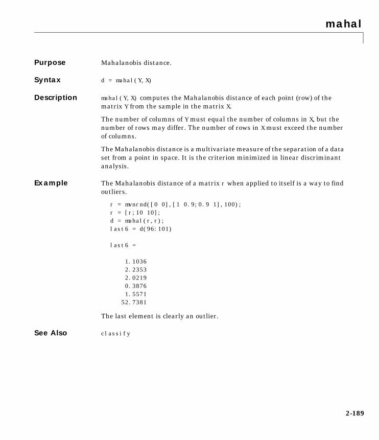
mahal
2-189
2mahalPurpose Mahalanobis distance.
Syntax d = mahal(Y,X)
Description mahal(Y,X) computes the Mahalanobis distance of each point (row) of thematrix Y from the sample in the matrix X.
The number of columns of Y must equal the number of columns in X, but thenumber of rows may differ. The number of rows in X must exceed the numberof columns.
The Mahalanobis distance is a multivariate measure of the separation of a dataset from a point in space. It is the criterion minimized in linear discriminantanalysis.
Example The Mahalanobis distance of a matrix r when applied to itself is a way to findoutliers.
r = mvnrnd([0 0],[1 0.9;0.9 1],100);r = [r;10 10];d = mahal(r,r);last6 = d(96:101)
last6 =
1.1036 2.2353 2.0219 0.3876 1.5571 52.7381
The last element is clearly an outlier.
See Also classify
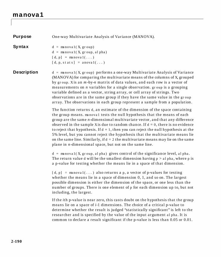
manova1
2-190
2manova1Purpose One-way Multivariate Analysis of Variance (MANOVA).
Syntax d = manova1(X,group)d = manova1(X,group,alpha)[d,p] = manova1(...)[d,p,stats] = anova1(...)
Description d = manova1(X,group) performs a one-way Multivariate Analysis of Variance(MANOVA) for comparing the multivariate means of the columns of X, groupedby group. X is an m-by-n matrix of data values, and each row is a vector ofmeasurements on n variables for a single observation. group is a groupingvariable defined as a vector, string array, or cell array of strings. Twoobservations are in the same group if they have the same value in the grouparray. The observations in each group represent a sample from a population.
The function returns d, an estimate of the dimension of the space containingthe group means. manova1 tests the null hypothesis that the means of eachgroup are the same n-dimensional multivariate vector, and that any differenceobserved in the sample X is due to random chance. If d = 0, there is no evidenceto reject that hypothesis. If d = 1, then you can reject the null hypothesis at the5% level, but you cannot reject the hypothesis that the multivariate means lieon the same line. Similarly, if d = 2 the multivariate means may lie on the sameplane in n-dimensional space, but not on the same line.
d = manova1(X,group,alpha) gives control of the significance level, alpha.The return value d will be the smallest dimension having p > alpha, where p isa p-value for testing whether the means lie in a space of that dimension.
[d,p] = manova1(...) also returns a p, a vector of p-values for testingwhether the means lie in a space of dimension 0, 1, and so on. The largestpossible dimension is either the dimension of the space, or one less than thenumber of groups. There is one element of p for each dimension up to, but notincluding, the largest.
If the ith p-value is near zero, this casts doubt on the hypothesis that the groupmeans lie on a space of i-1 dimensions. The choice of a critical p-value todetermine whether the result is judged “statistically significant” is left to theresearcher and is specified by the value of the input argument alpha. It iscommon to declare a result significant if the p-value is less than 0.05 or 0.01.

manova1
2-191
[d,p,stats] = anova1(...) also returns stats, a structure containingadditional MANOVA results. The structure contains the following fields.
The canonical variables C are linear combinations of the original variables,chosen to maximize the separation between groups. Specifically, C(:,1) is thelinear combination of the X columns that has the maximum separation betweengroups. This means that among all possible linear combinations, it is the onewith the most significant F statistic in a one-way analysis of variance.
Field Contents
W Within-groups sum of squares and cross-products matrix
B Between-groups sum of squares and cross-products matrix
T Total sum of squares and cross-products matrix
dfW Degrees of freedom for W
dfB Degrees of freedom for B
dfT Degrees of freedom for T
lambda Vector of values of Wilk’s lambda test statistic for testingwhether the means have dimension 0, 1, etc.
chisq Transformation of lambda to an approximate chi-squaredistribution
chisqdf Degrees of freedom for chisq
eigenval Eigenvalues of
eigenvec Eigenvectors of ; these are the coefficients for thecanonical variables C, and they are scaled so the within-groupvariance of the canonical variables is 1
canon Canonical variables C, equal to XC*eigenvec, where XC is X withcolumns centered by subtracting their means
mdist A vector of Mahalanobis distances from each point to the meanof its group
gmdist A matrix of Mahalanobis distances between each pair of groupmeans
W 1– B
W 1– B

manova1
2-192
C(:,2) has the maximum separation subject to it being orthogonal to C(:,1),and so on.
You may find it useful to use the outputs from manova1 along with otherfunctions to supplement your analysis. For example, you may want to startwith a grouped scatter plot matrix of the original variables using gplotmatrix.You can use gscatter to visualize the group separation using the first twocanonical variables. You can use manovacluster to graph a dendrogramshowing the clusters among the group means.
AssumptionsThe MANOVA test makes the following assumptions about the data in X:
• The populations for each group are normally distributed.
• The variance-covariance matrix is the same for each population.
• All observations are mutually independent.
Example We can use manova1 to determine whether there are differences in the averagesof four car characteristics, among groups defined by the country where the carswere made.
load carbig[d,p] = manova1([MPG Acceleration Weight Displacement],Origin)
d = 3
p = 0 0.0000 0.0075 0.1934
There are four dimensions in the input matrix, so the group means must lie ina four-dimensional space. manova1 shows that we cannot reject the hypothesisthat the means lie in a three-dimensional subspace.

manova1
2-193
References Krzanowski, W. J. Principles of Multivariate Analysis. Oxford UniversityPress, 1988.
See Also anova1, gscatter, gplotmatrix, manovacluster
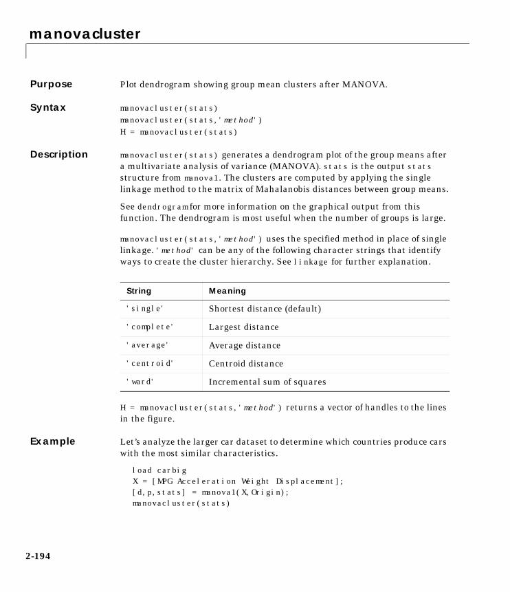
manovacluster
2-194
2manovaclusterPurpose Plot dendrogram showing group mean clusters after MANOVA.
Syntax manovacluster(stats)manovacluster(stats,'method')H = manovacluster(stats)
Description manovacluster(stats) generates a dendrogram plot of the group means aftera multivariate analysis of variance (MANOVA). stats is the output statsstructure from manova1. The clusters are computed by applying the singlelinkage method to the matrix of Mahalanobis distances between group means.
See dendrogram for more information on the graphical output from thisfunction. The dendrogram is most useful when the number of groups is large.
manovacluster(stats,'method') uses the specified method in place of singlelinkage. 'method' can be any of the following character strings that identifyways to create the cluster hierarchy. See linkage for further explanation.
H = manovacluster(stats,'method') returns a vector of handles to the linesin the figure.
Example Let’s analyze the larger car dataset to determine which countries produce carswith the most similar characteristics.
load carbigX = [MPG Acceleration Weight Displacement];[d,p,stats] = manova1(X,Origin);manovacluster(stats)
String Meaning
'single' Shortest distance (default)
'complete' Largest distance
'average' Average distance
'centroid' Centroid distance
'ward' Incremental sum of squares

manovacluster
2-195
See Also cluster, dendrogram, linkage, manova1
Japan Germany Italy France Sweden England USA 0
0.5
1
1.5
2
2.5
3

mean
2-196
2meanPurpose Average or mean value of vectors and matrices.
Syntax m = mean(X)
Description m = mean(X) calculates the sample average
For vectors, mean(x) is the mean value of the elements in vector x. Formatrices, mean(X) is a row vector containing the mean value of each column.
The mean function is part of the standard MATLAB language.
Example These commands generate five samples of 100 normal random numbers withmean, zero, and standard deviation, one. The sample averages in xbar aremuch less variable (0.00 ± 0.10).
x = normrnd(0,1,100,5);xbar = mean(x)
xbar =
0.0727 0.0264 0.0351 0.0424 0.0752
See Also median, std, cov, corrcoef, var
xj1n--- xij
i 1=
n
�=
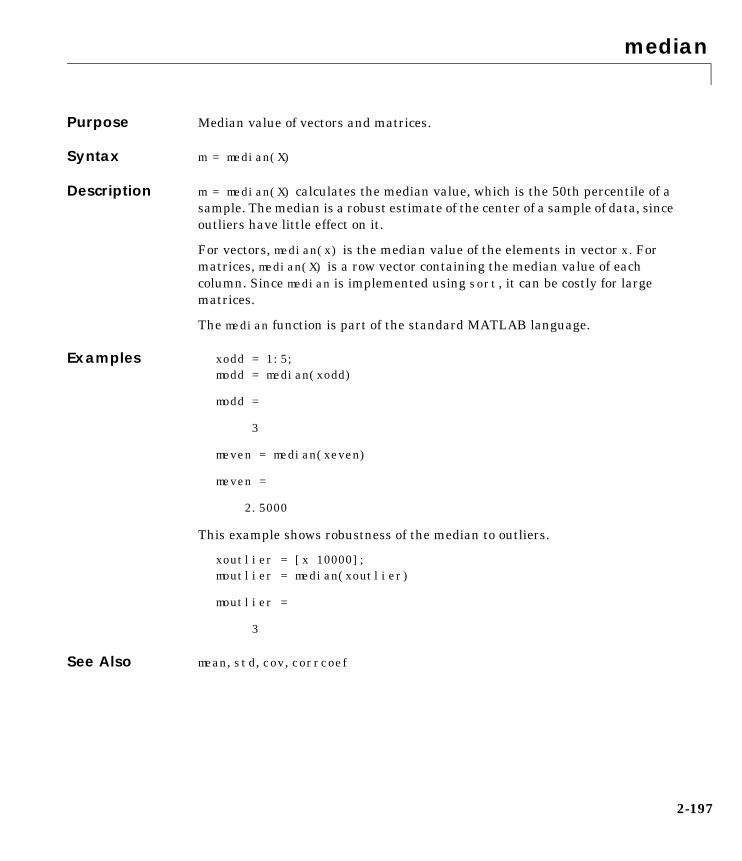
median
2-197
2medianPurpose Median value of vectors and matrices.
Syntax m = median(X)
Description m = median(X) calculates the median value, which is the 50th percentile of asample. The median is a robust estimate of the center of a sample of data, sinceoutliers have little effect on it.
For vectors, median(x) is the median value of the elements in vector x. Formatrices, median(X) is a row vector containing the median value of eachcolumn. Since median is implemented using sort, it can be costly for largematrices.
The median function is part of the standard MATLAB language.
Examples xodd = 1:5;modd = median(xodd)
modd =
3
meven = median(xeven)
meven =
2.5000
This example shows robustness of the median to outliers.
xoutlier = [x 10000];moutlier = median(xoutlier)
moutlier =
3
See Also mean, std, cov, corrcoef
mle
2-198
2mlePurpose Maximum likelihood estimation.
Syntax phat = mle('dist',data)[phat,pci] = mle('dist',data)[phat,pci] = mle('dist',data,alpha)[phat,pci] = mle('dist',data,alpha,p1)
Description phat = mle('dist',data) returns the maximum likelihood estimates (MLEs)for the distribution specified in 'dist' using the sample in the vector, data.See “Overview of the Distributions” on page 1-12 for the list of availabledistributions.
[phat,pci] = mle('dist',data) returns the MLEs and 95% percentconfidence intervals.
[phat,pci] = mle('dist',data,alpha) returns the MLEs and100(1-alpha)% confidence intervals given the data and the specified alpha.
[phat,pci] = mle('dist',data,alpha,p1) is used for the binomialdistribution only, where p1 is the number of trials.
Example rv = binornd(20,0.75)
rv = 16
[p,pci] = mle('binomial',rv,0.05,20)
p = 0.8000
pci = 0.5634 0.9427
See Also betafit, binofit, expfit, gamfit, normfit, poissfit, weibfit

moment
2-199
2momentPurpose Central moment of all orders.
Syntax m = moment(X,order)
Description m = moment(X,order) returns the central moment of X specified by thepositive integer order. For vectors, moment(x,order) returns the centralmoment of the specified order for the elements of x. For matrices,moment(X,order) returns central moment of the specified order for eachcolumn.
Note that the central first moment is zero, and the second central moment isthe variance computed using a divisor of n rather than n-1, where n is thelength of the vector x or the number of rows in the matrix X.
The central moment of order k of a distribution is defined as
where E(x) is the expected value of x.
Example X = randn([6 5])
X = 1.1650 0.0591 1.2460 -1.2704 -0.0562 0.6268 1.7971 -0.6390 0.9846 0.5135 0.0751 0.2641 0.5774 -0.0449 0.3967 0.3516 0.8717 -0.3600 -0.7989 0.7562 -0.6965 -1.4462 -0.1356 -0.7652 0.4005 1.6961 -0.7012 -1.3493 0.8617 -1.3414
m = moment(X,3)
m = -0.0282 0.0571 0.1253 0.1460 -0.4486
See Also kurtosis, mean, skewness, std, var
mn E x µ–( )k=

multcompare
2-200
2multcomparePurpose Multiple comparison test of means or other estimates.
Syntax c = multcompare(stats)c = multcompare(stats,alpha)c = multcompare(stats,alpha,'displayopt')c = multcompare(stats,alpha,'displayopt','ctype')c = multcompare(stats,alpha,'displayopt','ctype','estimate')c = multcompare(stats,alpha,'displayopt','ctype','estimate',dim)[c,m] = multcompare(...)[c,m,h] = multcompare(...)
Description c = multcompare(stats) performs a multiple comparison test using theinformation in the stats structure, and returns a matrix c of pairwisecomparison results. It also displays an interactive figure presenting agraphical representation of the test.
In a one-way analysis of variance, you compare the means of several groups totest the hypothesis that they are all the same, against the general alternativethat they are not all the same. Sometimes this alternative may be too general.You may need information about which pairs of means are significantlydifferent, and which are not. A test that can provide such information is calleda “multiple comparison procedure.”
When you perform a simple t-test of one group mean against another, youspecify a significance level that determines the cutoff value of the t statistic.For example, you can specify the value alpha = 0.05 to insure that when thereis no real difference, you will incorrectly find a significant difference no morethan 5% of the time. When there are many group means, there are also manypairs to compare. If you applied an ordinary t-test in this situation, the alphavalue would apply to each comparison, so the chance of incorrectly finding asignificant difference would increase with the number of comparisons. Multiplecomparison procedures are designed to provide an upper bound on theprobability that any comparison will be incorrectly found significant.
The output c contains the results of the test in the form of a five-column matrix.Each row of the matrix represents one test, and there is one row for each pairof groups. The entries in the row indicate the means being compared, theestimated difference in means, and a confidence interval for the difference.

multcompare
2-201
For example, suppose one row contains the following entries.
2.0000 5.0000 1.9442 8.2206 14.4971
These numbers indicate that the mean of group 2 minus the mean of group 5 isestimated to be 8.2206, and a 95% confidence interval for the true mean is[1.9442, 14.4971].
In this example the confidence interval does not contain 0.0, so the differenceis significant at the 0.05 level. If the confidence interval did contain 0.0, thedifference would not be significant at the 0.05 level.
The multcompare function also displays a graph with each group meanrepresented by a symbol and an interval around the symbol. Two means aresignificantly different if their intervals are disjoint, and are not significantlydifferent if their intervals overlap. You can use the mouse to select any group,and the graph will highlight any other groups that are significantly differentfrom it.
c = multcompare(stats,alpha) determines the confidence levels of theintervals in the c matrix and in the figure. The confidence level is100*(1-alpha)%. The default value of alpha is 0.05.
c = multcompare(stats,alpha,'displayopt') enables the graph displaywhen 'displayopt' is 'on' (default) and suppresses the display when'displayopt' is 'off'.

multcompare
2-202
c = multcompare(stats,alpha,'displayopt','ctype') specifies the criticalvalue to use for the multiple comparison, which can be any of the following.
ctype Meaning
'hsd' Use Tukey's honestly significant difference criterion.This is the default, and it is based on the Studentizedrange distribution. It is optimal for balanced one-wayANOVA and similar procedures with equal sample sizes.It has been proven to be conservative for one-wayANOVA with different sample sizes. According to theunproven Tukey-Kramer conjecture, it is also accuratefor problems where the quantities being compared arecorrelated, as in analysis of covariance with unbalancedcovariate values.
'lsd' Use Tukey's least significant difference procedure. Thisprocedure is a simple t-test. It is reasonable if thepreliminary test (say, the one-way ANOVA F statistic)shows a significant difference. If it is usedunconditionally, it provides no protection againstmultiple comparisons.
'bonferroni' Use critical values from the t distribution, after aBonferroni adjustment to compensate for multiplecomparisons. This procedure is conservative, but usuallyless so than the Scheffé procedure.
'dunn-sidak' Use critical values from the t distribution, after anadjustment for multiple comparisons that was proposedby Dunn and proved accurate by Šidák. This procedure issimilar to, but less conservative than, the Bonferroniprocedure.
'scheffe' Use critical values from Scheffé’s S procedure, derivedfrom the F distribution. This procedure provides asimultaneous confidence level for comparisons of alllinear combinations of the means, and it is conservativefor comparisons of simple differences of pairs.

multcompare
2-203
c = multcompare(stats,alpha,'displayopt','ctype','estimate')specifies the estimate to be compared. The allowable values of estimate dependon the function that was the source of the stats structure, according to thefollowing table.
c = multcompare(stats,alpha,'displayopt','ctype','estimate',dim)specifies the population marginal means to be compared. This argument isused only if the input stats structure was created by the anovan function. Forn-way ANOVA with n factors, you can specify dim as a scalar or a vector ofintegers between 1 and n. The default value is 1.
For example, if dim = 1, the estimates that are compared are the means foreach value of the first grouping variable, adjusted by removing effects of theother grouping variables as if the design were balanced. If dim = [1 3],population marginal means are computed for each combination of the first andthird grouping variables, removing effects of the second grouping variable. Ifyou fit a singular model, some cell means may not be estimable and anypopulation marginal means that depend on those cell means will have thevalue NaN.
Source Allowable Values of Estimate
'anova1' Ignored. Always compare the group means.
'anova2' Either 'column' (the default) or 'row' to comparecolumn or row means.
'anovan' Ignored. Always compare the population marginalmeans as specified by the dim argument.
'aoctool' Either 'slope', 'intercept', or 'pmm' to compareslopes, intercepts, or population marginal means. Ifthe analysis of covariance model did not includeseparate slopes, then 'slope' is not allowed. If it didnot include separate intercepts, then no comparisonsare possible.
'friedman' Ignored. Always compare average column ranks.
'kruskalwallis' Ignored. Always compare average group ranks.

multcompare
2-204
Population marginal means are described by Milliken and Johnson (1992) andby Searle, Speed, and Milliken (1980). The idea behind population marginalmeans is to remove any effect of an unbalanced design by fixing the values ofthe factors specified by dim, and averaging out the effects of other factors as ifeach factor combination occurred the same number of times. The definition ofpopulation marginal means does not depend on the number of observations ateach factor combination. For designed experiments where the number ofobservations at each factor combination has no meaning, population marginalmeans can be easier to interpret than simple means ignoring other factors. Forsurveys and other studies where the number of observations at eachcombination does have meaning, population marginal means may be harder tointerpret.
[c,m] = multcompare(...) returns an additional matrix m. The first columnof m contains the estimated values of the means (or whatever statistics arebeing compared) for each group, and the second column contains their standarderrors.
[c,m,h] = multcompare(...) returns a handle h to the comparison graph.Note that the title of this graph contains instructions for interacting with thegraph, and the x-axis label contains information about which means aresignificantly different from the selected mean. If you plan to use this graph forpresentation, you may want to omit the title and the x-axis label. You canremove them using interactive features of the graph window, or you can use thefollowing commands.
title('')xlabel('')
Example Let’s revisit the anova1 example testing the material strength in structuralbeams. From the anova1 output we found significant evidence that the threetypes of beams are not equivalent in strength. Now we can determine wherethose differences lie. First we create the data arrays and we perform one-wayANOVA.
strength = [82 86 79 83 84 85 86 87 74 82 78 75 76 77 79 ... 79 77 78 82 79];alloy = {'st','st','st','st','st','st','st','st',... 'al1','al1','al1','al1','al1','al1',... 'al2','al2','al2','al2','al2','al2'};

multcompare
2-205
[p,a,s] = anova1(strength,alloy);
Among the outputs is a structure that we can use as input to multcompare.
multcompare(s)
ans = 1.0000 2.0000 3.6064 7.0000 10.3936 1.0000 3.0000 1.6064 5.0000 8.3936 2.0000 3.0000 -5.6280 -2.0000 1.6280
The third row of the output matrix shows that the differences in strengthbetween the two alloys is not significant. A 95% confidence interval for thedifference is [-5.6, 1.6], so we cannot reject the hypothesis that the truedifference is zero.
The first two rows show that both comparisons involving the first group (steel)have confidence intervals that do not include zero. In other words, thosedifferences are significant. The graph shows the same information.
See Also anova1, anova2, anovan, aoctool, friedman, kruskalwallis
74 76 78 80 82 84 86
al2
al1
st
Click on the group you want to test
2 groups have slopes significantly different from st

multcompare
2-206
References Hochberg, Y., and A. C. Tamhane, Multiple Comparison Procedures, 1987,Wiley.
Milliken, G. A., and D. E. Johnson, Analysis of Messy Data, Volume 1: DesignedExperiments, 1992, Chapman & Hall.
Searle, S. R., F. M. Speed, and G. A. Milliken, “Population marginal means inthe linear model: an alternative to least squares means,” AmericanStatistician, 1980, pp. 216-221.
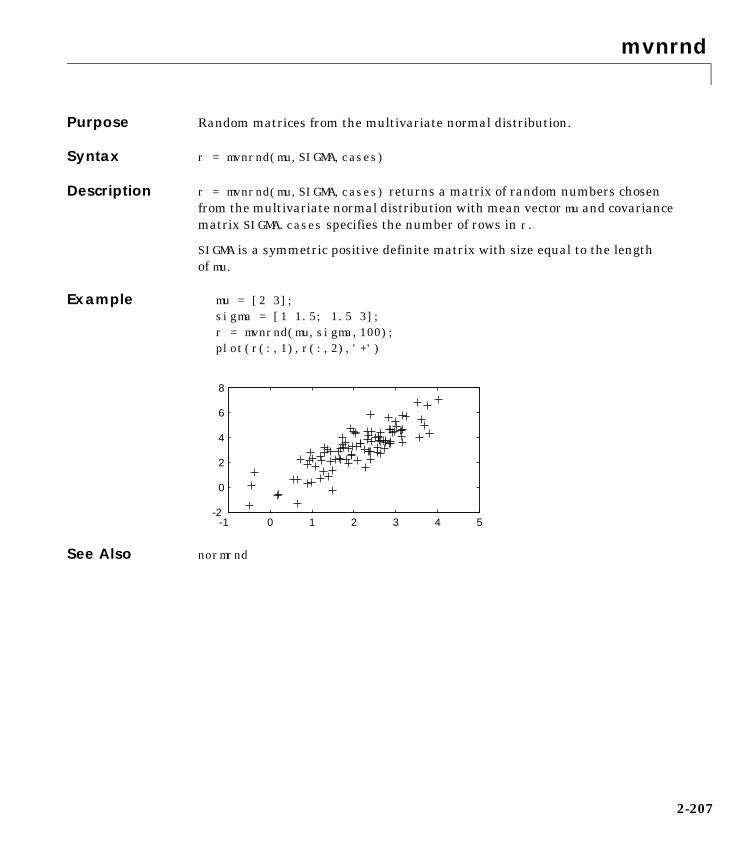
mvnrnd
2-207
2mvnrndPurpose Random matrices from the multivariate normal distribution.
Syntax r = mvnrnd(mu,SIGMA,cases)
Description r = mvnrnd(mu,SIGMA,cases) returns a matrix of random numbers chosenfrom the multivariate normal distribution with mean vector mu and covariancematrix SIGMA. cases specifies the number of rows in r.
SIGMA is a symmetric positive definite matrix with size equal to the lengthof mu.
Example mu = [2 3];sigma = [1 1.5; 1.5 3];r = mvnrnd(mu,sigma,100);plot(r(:,1),r(:,2),'+')
See Also normrnd
-1 0 1 2 3 4 5-2
0
2
4
6
8

mvtrnd
2-208
2mvtrndPurpose Random matrices from the multivariate t distribution.
Syntax r = mvtrnd(C,df,cases)
Description r = mvtrnd(C,df,cases) returns a matrix of random numbers chosen fromthe multivariate t distribution, where C is a correlation matrix. df is thedegrees of freedom and is either a scalar or is a vector with cases elements. Ifp is the number of columns in C, then the output r has cases rows and pcolumns.
Let t represent a row of r. Then the distribution of t is that of a vector havinga multivariate normal distribution with mean 0, variance 1, and covariancematrix C, divided by an independent chi-square random value having df degrees of freedom. The rows of r are independent.
C must be a square, symmetric and positive definite matrix. If its diagonalelements are not all 1 (that is, if C is a covariance matrix rather than acorrelation matrix), mvtrnd computes the equivalent correlation matrix beforegenerating the random numbers.
Example sigma = [1 0.8;0.8 1];r = mvtrnd(sigma,3,100);plot(r(:,1),r(:,2),'+')
See Also mvnrnd, trnd
−4 −2 0 2 4 6 8 10 12−4
−2
0
2
4
6
8
10

nanmax
2-209
2nanmaxPurpose Maximum ignoring NaNs.
Syntax m = nanmax(a)[m,ndx] = nanmax(a)m = nanmax(a,b)
Description m = nanmax(a) returns the maximum with NaNs treated as missing. Forvectors, nanmax(a) is the largest non-NaN element in a. For matrices,nanmax(A) is a row vector containing the maximum non-NaN element from eachcolumn.
[m,ndx] = nanmax(a) also returns the indices of the maximum values invector ndx.
m = nanmax(a,b) returns the larger of a or b, which must match in size.
Example m = magic(3);m([1 6 8]) = [NaN NaN NaN]
m =
NaN 1 6 3 5 NaN 4 NaN 2
[nmax,maxidx] = nanmax(m)
nmax =
4 5 6
maxidx =
3 2 1
See Also nanmin, nanmean, nanmedian, nanstd, nansum

nanmean
2-210
2nanmeanPurpose Mean ignoring NaNs
Syntax y = nanmean(X)
Description y = nanmean(X) is the average computed by treating NaNs as missing values.
For vectors, nanmean(x) is the mean of the non-NaN elements of x. For matrices,nanmean(X) is a row vector containing the mean of the non-NaN elements ineach column.
Example m = magic(3);m([1 6 8]) = [NaN NaN NaN]
m =
NaN 1 6 3 5 NaN 4 NaN 2
nmean = nanmean(m)
nmean =
3.5000 3.0000 4.0000
See Also nanmin, nanmax, nanmedian, nanstd, nansum
nanmedian
2-211
2nanmedianPurpose Median ignoring NaNs
Syntax y = nanmedian(X)
Description y = nanmedian(X) is the median computed by treating NaNs as missing values.
For vectors, nanmedian(x) is the median of the non-NaN elements of x. Formatrices, nanmedian(X) is a row vector containing the median of the non-NaNelements in each column of X.
Example m = magic(4);m([1 6 9 11]) = [NaN NaN NaN NaN]
m =
NaN 2 NaN 13 5 NaN 10 8 9 7 NaN 12 4 14 15 1
nmedian = nanmedian(m)
nmedian =
5.0000 7.0000 12.5000 10.0000
See Also nanmin, nanmax, nanmean, nanstd, nansum
nanmin
2-212
2nanminPurpose Minimum ignoring NaNs
Syntax m = nanmin(a)[m,ndx] = nanmin(a)m = nanmin(a,b)
Description m = nanmin(a) is the minimum computed by treating NaNs as missing values.For vectors, nanmin(a) is the smallest non-NaN element in a. For matrices,nanmin(A) is a row vector containing the minimum non-NaN element from eachcolumn.
[m,ndx] = nanmin(a) also returns the indices of the minimum values invector ndx.
m = nanmin(a,b) returns the smaller of a or b, which must match in size.
Example m = magic(3);m([1 6 8]) = [NaN NaN NaN]
m =
NaN 1 6 3 5 NaN 4 NaN 2
[nmin,minidx] = nanmin(m)
nmin =
3 1 2
minidx =
2 1 3
See Also nanmax, nanmean, nanmedian, nanstd, nansum

nanstd
2-213
2nanstdPurpose Standard deviation ignoring NaNs.
Syntax y = nanstd(X)
Description y = nanstd(X) is the standard deviation computed by treating NaNs asmissing values.
For vectors, nanstd(x) is the standard deviation of the non-NaN elements of x.For matrices, nanstd(X) is a row vector containing the standard deviations ofthe non-NaN elements in each column of X.
Example m = magic(3);m([1 6 8]) = [NaN NaN NaN]
m =
NaN 1 6 3 5 NaN 4 NaN 2
nstd = nanstd(m)
nstd =
0.7071 2.8284 2.8284
See Also nanmax, nanmin, nanmean, nanmedian, nansum
nansum
2-214
2nansumPurpose Sum ignoring NaNs.
Syntax y = nansum(X)
Description y = nansum(X) is the sum computed by treating NaNs as missing values.
For vectors, nansum(x) is the sum of the non-NaN elements of x. For matrices,nansum(X) is a row vector containing the sum of the non-NaN elements in eachcolumn of X.
Example m = magic(3);m([1 6 8]) = [NaN NaN NaN]
m =
NaN 1 6 3 5 NaN 4 NaN 2
nsum = nansum(m)
nsum =
7 6 8
See Also nanmax, nanmin, nanmean, nanmedian, nanstd
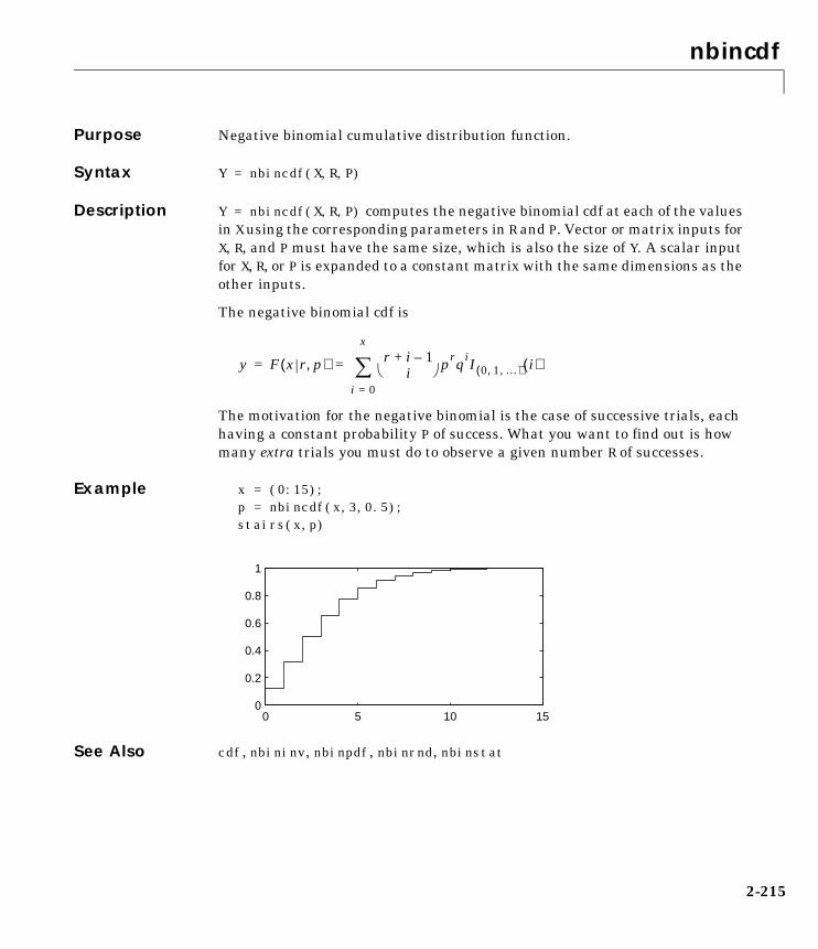
nbincdf
2-215
2nbincdfPurpose Negative binomial cumulative distribution function.
Syntax Y = nbincdf(X,R,P)
Description Y = nbincdf(X,R,P) computes the negative binomial cdf at each of the valuesin X using the corresponding parameters in R and P. Vector or matrix inputs forX, R, and P must have the same size, which is also the size of Y. A scalar inputfor X, R, or P is expanded to a constant matrix with the same dimensions as theother inputs.
The negative binomial cdf is
The motivation for the negative binomial is the case of successive trials, eachhaving a constant probability P of success. What you want to find out is howmany extra trials you must do to observe a given number R of successes.
Example x = (0:15);p = nbincdf(x,3,0.5);stairs(x,p)
See Also cdf, nbininv, nbinpdf, nbinrnd, nbinstat
y F x r p,( ) r i 1–+i� �
� �
i 0=
x
� prqiI 0 1 …, ,( ) i( )= =
0 5 10 150
0.2
0.4
0.6
0.8
1

nbininv
2-216
2nbininvPurpose Inverse of the negative binomial cumulative distribution function (cdf).
Syntax X = nbininv(Y,R,P)
Description X = nbininv(Y,R,P) returns the inverse of the negative binomial cdf withparameters R and P at the corresponding probabilities in P. Since the binomialdistribution is discrete, nbininv returns the least integer X such that thenegative binomial cdf evaluated at X equals or exceeds Y. Vector or matrixinputs for Y, R, and P must have the same size, which is also the size of X. Ascalar input for Y, R, or P is expanded to a constant matrix with the samedimensions as the other inputs.
The negative binomial cdf models consecutive trials, each having a constantprobability P of success. The parameter R is the number of successes requiredbefore stopping.
Example How many times would you need to flip a fair coin to have a 99% probability ofhaving observed 10 heads?
flips = nbininv(0.99,10,0.5) + 10
flips =
33
Note that you have to flip at least 10 times to get 10 heads. That is why thesecond term on the right side of the equals sign is a 10.
See Also icdf, nbincdf, nbinpdf, nbinrnd, nbinstat

nbinpdf
2-217
2nbinpdfPurpose Negative binomial probability density function.
Syntax Y = nbinpdf(X,R,P)
Description Y = nbinpdf(X,R,P) returns the negative binomial pdf at each of the valuesin X using the corresponding parameters in R and P. Vector or matrix inputs forX, R, and P must have the same size, which is also the size of Y. A scalar inputfor X, R, or P is expanded to a constant matrix with the same dimensions as theother inputs. Note that the density function is zero unless the values in X areintegers.
The negative binomial pdf is
The negative binomial pdf models consecutive trials, each having a constantprobability P of success. The parameter R is the number of successes requiredbefore stopping.
Example x = (0:10);y = nbinpdf(x,3,0.5);plot(x,y,'+')set(gca,'Xlim',[-0.5,10.5])
See Also nbincdf, nbininv, nbinrnd, nbinstat, pdf
y f x r p,( ) r x 1–+x� �
� � prqxI 0 1 …, ,( ) x( )= =
0 2 4 6 8 100
0.05
0.1
0.15
0.2

nbinrnd
2-218
2nbinrndPurpose Random matrices from a negative binomial distribution.
Syntax RND = nbinrnd(R,P)RND = nbinrnd(R,P,m)RND = nbinrnd(R,P,m,n)
Description RND = nbinrnd(R,P) is a matrix of random numbers chosen from a negativebinomial distribution with parameters R and P. Vector or matrix inputs for Rand P must have the same size, which is also the size of RND. A scalar input forR or P is expanded to a constant matrix with the same dimensions as the otherinput.
RND = nbinrnd(R,P,m) generates random numbers with parameters R and P,where m is a 1-by-2 vector that contains the row and column dimensions of RND.
RND = nbinrnd(R,P,m,n) generates random numbers with parameters Rand P, where scalars m and n are the row and column dimensions of RND.
The negative binomial distribution models consecutive trials, each having aconstant probability P of success. The parameter R is the number of successesrequired before stopping.
Example Suppose you want to simulate a process that has a defect probability of 0.01.How many units might Quality Assurance inspect before finding threedefective items?
r = nbinrnd(3,0.01,1,6) + 3
r =
496 142 420 396 851 178
See Also nbincdf, nbininv, nbinpdf, nbinstat

nbinstat
2-219
2nbinstatPurpose Mean and variance of the negative binomial distribution.
Syntax [M,V] = nbinstat(R,P)
Description [M,V] = nbinstat(R,P) returns the mean and variance of the negativebinomial distribution with parameters R and P. Vector or matrix inputs for Rand P must have the same size, which is also the size of M and V. A scalar inputfor R or P is expanded to a constant matrix with the same dimensions as theother input.
The mean of the negative binomial distribution with parameters r and p is rq/p,where q = 1-p. The variance is rq/p2.
Example p = 0.1:0.2:0.9;r = 1:5;[R,P] = meshgrid(r,p);[M,V] = nbinstat(R,P)
M =
9.0000 18.0000 27.0000 36.0000 45.0000 2.3333 4.6667 7.0000 9.3333 11.6667 1.0000 2.0000 3.0000 4.0000 5.0000 0.4286 0.8571 1.2857 1.7143 2.1429 0.1111 0.2222 0.3333 0.4444 0.5556
V =
90.0000 180.0000 270.0000 360.0000 450.0000 7.7778 15.5556 23.3333 31.1111 38.8889 2.0000 4.0000 6.0000 8.0000 10.0000 0.6122 1.2245 1.8367 2.4490 3.0612 0.1235 0.2469 0.3704 0.4938 0.6173
See Also nbincdf, nbininv, nbinpdf, nbinrnd

ncfcdf
2-220
2ncfcdfPurpose Noncentral F cumulative distribution function (cdf).
Syntax P = ncfcdf(X,NU1,NU2,DELTA)
Description P = ncfcdf(X,NU1,NU2,DELTA) computes the noncentral F cdf at each of thevalues in X using the corresponding numerator degrees of freedom in NU1,denominator degrees of freedom in NU2, and positive noncentrality parametersin DELTA. Vector or matrix inputs for X, NU1, NU2, and DELTAmust have the samesize, which is also the size of P. A scalar input for X, NU1, NU2, or DELTA isexpanded to a constant matrix with the same dimensions as the other inputs.
The noncentral F cdf is
where I(x|a,b) is the incomplete beta function with parameters a and b.
Example Compare the noncentral F cdf with δ = 10 to the F cdf with the same number ofnumerator and denominator degrees of freedom (5 and 20 respectively).
x = (0.01:0.1:10.01)';p1 = ncfcdf(x,5,20,10);p = fcdf(x,5,20);plot(x,p,'--',x,p1,'-')
F x ν1 ν2 δ, ,( )
12---δ� �� �
j
j!--------------e
δ2---–
� �� �� �� �� �
Iν1 x⋅
ν2 ν+1 x⋅
-------------------------ν12------ j+
ν22------,
� �� �� �
j 0=
∞
�=
0 2 4 6 8 10 120
0.2
0.4
0.6
0.8
1

ncfcdf
2-221
References Johnson, N., and S. Kotz, Distributions in Statistics: Continuous UnivariateDistributions-2, John Wiley and Sons, 1970. pp. 189–200.
See Also cdf, ncfpdf, ncfinv, ncfrnd, ncfstat

ncfinv
2-222
2ncfinvPurpose Inverse of the noncentral F cumulative distribution function (cdf).
Syntax X = ncfinv(P,NU1,NU2,DELTA)
Description X = ncfinv(P,NU1,NU2,DELTA) returns the inverse of the noncentral F cdfwith numerator degrees of freedom NU1, denominator degrees of freedom NU2,and positive noncentrality parameter DELTA for the corresponding probabilitiesin P. Vector or matrix inputs for P, NU1, NU2, and DELTA must have the samesize, which is also the size of X. A scalar input for P, NU1, NU2, or DELTA isexpanded to a constant matrix with the same dimensions as the other inputs.
Example One hypothesis test for comparing two sample variances is to take their ratioand compare it to an F distribution. If the numerator and denominator degreesof freedom are 5 and 20 respectively, then you reject the hypothesis that thefirst variance is equal to the second variance if their ratio is less than thatcomputed below.
critical = finv(0.95,5,20)
critical =
2.7109
Suppose the truth is that the first variance is twice as big as the secondvariance. How likely is it that you would detect this difference?
prob = 1 - ncfcdf(critical,5,20,2)
prob =
0.1297
References Evans, M., N. Hastings, and B. Peacock, Statistical Distributions, SecondEdition, John Wiley and Sons, 1993. p. 102–105.
Johnson, N., and S. Kotz, Distributions in Statistics: Continuous UnivariateDistributions-2, John Wiley and Sons, 1970. pp. 189–200.
See Also icdf, ncfcdf, ncfpdf, ncfrnd, ncfstat
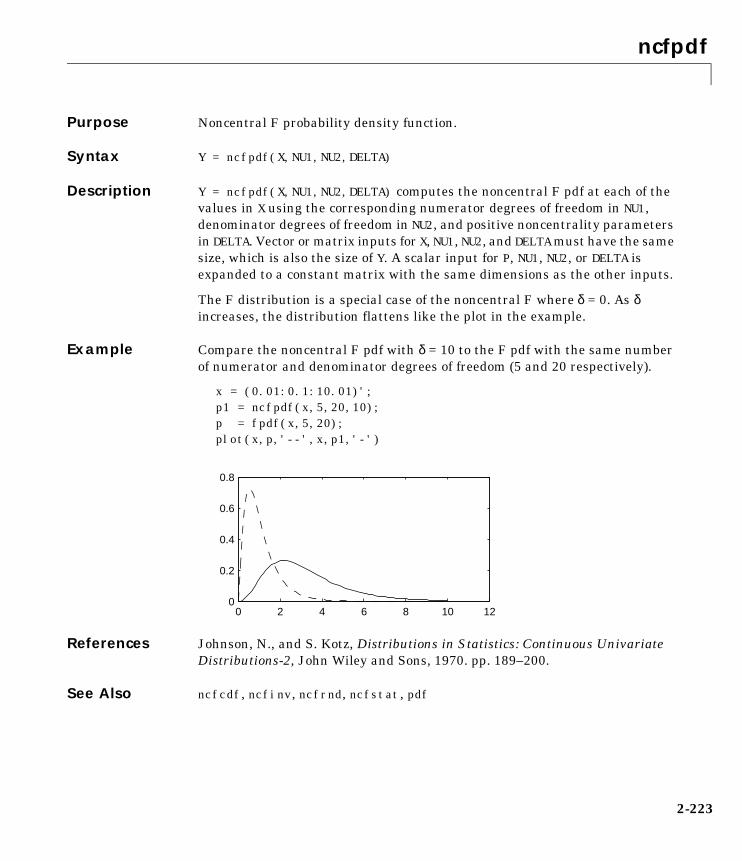
ncfpdf
2-223
2ncfpdfPurpose Noncentral F probability density function.
Syntax Y = ncfpdf(X,NU1,NU2,DELTA)
Description Y = ncfpdf(X,NU1,NU2,DELTA) computes the noncentral F pdf at each of thevalues in X using the corresponding numerator degrees of freedom in NU1,denominator degrees of freedom in NU2, and positive noncentrality parametersin DELTA. Vector or matrix inputs for X, NU1, NU2, and DELTA must have the samesize, which is also the size of Y. A scalar input for P, NU1, NU2, or DELTA isexpanded to a constant matrix with the same dimensions as the other inputs.
The F distribution is a special case of the noncentral F where δ = 0. As δincreases, the distribution flattens like the plot in the example.
Example Compare the noncentral F pdf with δ = 10 to the F pdf with the same numberof numerator and denominator degrees of freedom (5 and 20 respectively).
x = (0.01:0.1:10.01)';p1 = ncfpdf(x,5,20,10);p = fpdf(x,5,20);plot(x,p,'--',x,p1,'-')
References Johnson, N., and S. Kotz, Distributions in Statistics: Continuous UnivariateDistributions-2, John Wiley and Sons, 1970. pp. 189–200.
See Also ncfcdf, ncfinv, ncfrnd, ncfstat, pdf
0 2 4 6 8 10 120
0.2
0.4
0.6
0.8

ncfrnd
2-224
2ncfrndPurpose Random matrices from the noncentral F distribution.
Syntax R = ncfrnd(NU1,NU2,DELTA)R = ncfrnd(NU1,NU2,DELTA,m)R = ncfrnd(NU1,NU2,DELTA,m,n)
Description R = ncfrnd(NU1,NU2,DELTA) returns a matrix of random numbers chosen fromthe noncentral F distribution with parameters NU1, NU2 and DELTA. Vector ormatrix inputs for NU1, NU2, and DELTA must have the same size, which is alsothe size of R. A scalar input for NU1, NU2, or DELTA is expanded to a constantmatrix with the same dimensions as the other inputs.
R = ncfrnd(NU1,NU2,DELTA,m) returns a matrix of random numbers withparameters NU1, NU2, and DELTA, where m is a 1-by-2 vector that contains therow and column dimensions of R.
R = ncfrnd(NU1,NU2,DELTA,m,n) generates random numbers withparameters NU1, NU2, and DELTA, where scalars m and n are the row and columndimensions of R.
Example Compute six random numbers from a noncentral F distribution with 10numerator degrees of freedom, 100 denominator degrees of freedom and anoncentrality parameter, δ, of 4.0. Compare this to the F distribution with thesame degrees of freedom.
r = ncfrnd(10,100,4,1,6)
r = 2.5995 0.8824 0.8220 1.4485 1.4415 1.4864
r1 = frnd(10,100,1,6)
r1 = 0.9826 0.5911 1.0967 0.9681 2.0096 0.6598
References Johnson, N., and S. Kotz, Distributions in Statistics: Continuous UnivariateDistributions-2, John Wiley and Sons, 1970. pp. 189–200.
See Also ncfcdf, ncfinv, ncfpdf, ncfstat

ncfstat
2-225
2ncfstatPurpose Mean and variance of the noncentral F distribution.
Syntax [M,V] = ncfstat(NU1,NU2,DELTA)
Description [M,V] = ncfstat(NU1,NU2,DELTA) returns the mean and variance of thenoncentral F pdf with NU1 and NU2 degrees of freedom and noncentralityparameter DELTA. Vector or matrix inputs for NU1, NU2, and DELTA must havethe same size, which is also the size of M and V. A scalar input for NU1, NU2, orDELTA is expanded to a constant matrix with the same dimensions as the otherinput.
The mean of the noncentral F distribution with parameters ν1, ν2, and δ is
where ν2 > 2.
The variance is
where ν2 > 4.
Example [m,v]= ncfstat(10,100,4)
m = 1.4286
v = 3.9200
References Evans, M., N. Hastings, and B. Peacock, Statistical Distributions, SecondEdition, John Wiley and Sons, 1993. p. 73–74.
Johnson, N., and S. Kotz, Distributions in Statistics: Continuous UnivariateDistributions-2, John Wiley and Sons, 1970. pp. 189–200.
See Also ncfcdf, ncfinv, ncfpdf, ncfrnd
ν2 δ ν+ 1( )ν1 ν2 2–( )--------------------------
2ν2ν1------� �� �
2 δ ν+ 1( )2 2δ ν+ 1( ) ν2 2–( )+
ν2 2–( )2 ν2 4–( )--------------------------------------------------------------------------

nctcdf
2-226
2nctcdfPurpose Noncentral T cumulative distribution function.
Syntax P = nctcdf(X,NU,DELTA)
Description P = nctcdf(X,NU,DELTA) computes the noncentral T cdf at each of the valuesin X using the corresponding degrees of freedom in NU and noncentralityparameters in DELTA. Vector or matrix inputs for X, NU, and DELTA must havethe same size, which is also the size of P. A scalar input for X, NU, or DELTA isexpanded to a constant matrix with the same dimensions as the other inputs.
Example Compare the noncentral T cdf with DELTA = 1 to the T cdf with the samenumber of degrees of freedom (10).
x = (-5:0.1:5)';p1 = nctcdf(x,10,1);p = tcdf(x,10);plot(x,p,'--',x,p1,'-')
References Evans, M., N. Hastings, and B. Peacock, Statistical Distributions, SecondEdition, John Wiley and Sons, 1993. p. 147–148.
Johnson, N., and S. Kotz, Distributions in Statistics: Continuous UnivariateDistributions-2, John Wiley and Sons, 1970. pp. 201–219.
See Also cdf, nctcdf, nctinv, nctpdf, nctrnd, nctstat
-5 0 50
0.2
0.4
0.6
0.8
1

nctinv
2-227
2nctinvPurpose Inverse of the noncentral T cumulative distribution.
Syntax X = nctinv(P,NU,DELTA)
Description X = nctinv(P,NU,DELTA) returns the inverse of the noncentral T cdf with NUdegrees of freedom and noncentrality parameter DELTA for the correspondingprobabilities in P. Vector or matrix inputs for P, NU, and DELTA must have thesame size, which is also the size of X. A scalar input for P, NU, or DELTA isexpanded to a constant matrix with the same dimensions as the other inputs.
Example x = nctinv([0.1 0.2],10,1)
x = -0.2914 0.1618
References Evans, M., N. Hastings, and B. Peacock, Statistical Distributions, SecondEdition, John Wiley and Sons, 1993. p. 147–148.
Johnson, N., and S. Kotz, Distributions in Statistics: Continuous UnivariateDistributions-2, John Wiley and Sons, 1970. pp. 201–219.
See Also icdf, nctcdf, nctpdf, nctrnd, nctstat

nctpdf
2-228
2nctpdfPurpose Noncentral T probability density function (pdf).
Syntax Y = nctpdf(X,V,DELTA)
Description Y = nctpdf(X,V,DELTA) computes the noncentral T pdf at each of the valuesin X using the corresponding degrees of freedom in V and noncentralityparameters in DELTA. Vector or matrix inputs for X, V, and DELTAmust have thesame size, which is also the size of Y. A scalar input for X, V, or DELTA isexpanded to a constant matrix with the same dimensions as the other inputs.
Example Compare the noncentral T pdf with DELTA = 1 to the T pdf with the samenumber of degrees of freedom (10).
x = (-5:0.1:5)';p1 = nctpdf(x,10,1);p = tpdf(x,10);plot(x,p,'--',x,p1,'-')
References Evans, M., N. Hastings, and B. Peacock, Statistical Distributions, SecondEdition, John Wiley and Sons, 1993. p. 147–148.
Johnson, N., and S. Kotz, Distributions in Statistics: Continuous UnivariateDistributions-2, John Wiley and Sons, 1970. pp. 201–219.
See Also nctcdf, nctinv, nctrnd, nctstat, pdf
-5 0 50
0.1
0.2
0.3
0.4

nctrnd
2-229
2nctrndPurpose Random matrices from noncentral T distribution.
Syntax R = nctrnd(V,DELTA)R = nctrnd(V,DELTA,m)R = nctrnd(V,DELTA,m,n)
Description R = nctrnd(V,DELTA) returns a matrix of random numbers chosen from thenoncentral T distribution with parameters V and DELTA. Vector or matrixinputs for V and DELTA must have the same size, which is also the size of R. Ascalar input for V or DELTA is expanded to a constant matrix with the samedimensions as the other input.
R = nctrnd(V,DELTA,m) returns a matrix of random numbers withparameters V and DELTA, where m is a 1-by-2 vector that contains the row andcolumn dimensions of R.
R = nctrnd(V,DELTA,m,n) generates random numbers with parameters V andDELTA, where scalars m and n are the row and column dimensions of R.
Example nctrnd(10,1,5,1)
ans =
1.6576 1.0617 1.4491 0.2930 3.6297
References Evans, M., N. Hastings, and B. Peacock, Statistical Distributions, SecondEdition, John Wiley and Sons, 1993. p. 147–148.
Johnson, N., and S. Kotz, Distributions in Statistics: Continuous UnivariateDistributions-2, John Wiley and Sons, 1970. pp. 201–219.
See Also nctcdf, nctinv, nctpdf, nctstat

nctstat
2-230
2nctstatPurpose Mean and variance for the noncentral t distribution.
Syntax [M,V] = nctstat(NU,DELTA)
Description [M,V] = nctstat(NU,DELTA) returns the mean and variance of thenoncentral t pdf with NU degrees of freedom and noncentrality parameterDELTA. Vector or matrix inputs for NU and DELTAmust have the same size, whichis also the size of M and V. A scalar input for NU or DELTA is expanded to aconstant matrix with the same dimensions as the other input.
The mean of the noncentral t distribution with parameters ν and δ is
where ν > 1.
The variance is
where ν > 2.
Example [m,v] = nctstat(10,1)
m = 1.0837
v = 1.3255
References Evans, M., N. Hastings, and B. Peacock, Statistical Distributions, SecondEdition, John Wiley and Sons, 1993. p. 147–148.
Johnson, N., and S. Kotz, Distributions in Statistics: Continuous UnivariateDistributions-2, John Wiley and Sons, 1970. pp. 201–219.
See Also nctcdf, nctinv, nctpdf, nctrnd
δ ν 2⁄( )1 2⁄ Γ ν 1–( ) 2⁄( )Γ ν 2⁄( )
-------------------------------------------------------------
νν 2–( )
----------------- 1 δ2+( ) ν
2---– δ2 Γ ν 1–( ) 2⁄( )
Γ ν 2⁄( )---------------------------------
2

ncx2cdf
2-231
2ncx2cdfPurpose Noncentral chi-square cumulative distribution function (cdf).
Syntax P = ncx2cdf(X,V,DELTA)
Description P = ncx2cdf(X,V,DELTA) computes the noncentral chi-square cdf at each ofthe values in X using the corresponding degrees of freedom in V and positivenoncentrality parameters in DELTA. Vector or matrix inputs for X, V, and DELTAmust have the same size, which is also the size of P. A scalar input for X, V, orDELTA is expanded to a constant matrix with the same dimensions as the otherinputs.
Some texts refer to this distribution as the generalized Rayleigh,Rayleigh-Rice, or Rice distribution.
The noncentral chi-square cdf is
Example x = (0:0.1:10)';p1 = ncx2cdf(x,4,2);p = chi2cdf(x,4);plot(x,p,'--',x,p1,'-')
F x ν δ,( )
12---δ� �� �
j
j!--------------e
δ2---–
� �� �� �� �� �
Pr χν 2 j+
2 x≤[ ]
j 0=
∞
�=
0 2 4 6 8 100
0.2
0.4
0.6
0.8
1

ncx2cdf
2-232
References Johnson, N., and S. Kotz, Distributions in Statistics: Continuous UnivariateDistributions-2, John Wiley and Sons, 1970. pp. 130–148.
See Also cdf, ncx2inv, ncx2pdf, ncx2rnd, ncx2stat
ncx2inv
2-233
2ncx2invPurpose Inverse of the noncentral chi-square cdf.
Syntax X = ncx2inv(P,V,DELTA)
Description X = ncx2inv(P,V,DELTA) returns the inverse of the noncentral chi-square cdfwith parameters V and DELTA at the corresponding probabilities in P. Vector ormatrix inputs for P, V, and DELTAmust have the same size, which is also the sizeof X. A scalar input for P, V, or DELTA is expanded to a constant matrix with thesame dimensions as the other inputs.
Algorithm ncx2inv uses Newton's method to converge to the solution.
Example ncx2inv([0.01 0.05 0.1],4,2)
ans =
0.4858 1.1498 1.7066
References Evans, M., N. Hastings, and B. Peacock, Statistical Distributions, SecondEdition, John Wiley and Sons, 1993. p. 50–52.
Johnson, N., and S. Kotz, Distributions in Statistics: Continuous UnivariateDistributions-2, John Wiley and Sons, 1970. pp. 130–148.
See Also icdf, ncx2cdf, ncx2pdf, ncx2rnd, ncx2stat

ncx2pdf
2-234
2ncx2pdfPurpose Noncentral chi-square probability density function (pdf).
Syntax Y = ncx2pdf(X,V,DELTA)
Description Y = ncx2pdf(X,V,DELTA) computes the noncentral chi-square pdf at each ofthe values in X using the corresponding degrees of freedom in V and positivenoncentrality parameters in DELTA. Vector or matrix inputs for X, V, and DELTAmust have the same size, which is also the size of Y. A scalar input for X, V, orDELTA is expanded to a constant matrix with the same dimensions as the otherinputs.
Some texts refer to this distribution as the generalized Rayleigh,Rayleigh-Rice, or Rice distribution.
Example As the noncentrality parameter δ increases, the distribution flattens as shownin the plot.
x = (0:0.1:10)';p1 = ncx2pdf(x,4,2);p = chi2pdf(x,4);plot(x,p,'--',x,p1,'-')
References Johnson, N., and S. Kotz, Distributions in Statistics: Continuous UnivariateDistributions-2, John Wiley and Sons, 1970. pp. 130–148.
See Also ncx2cdf, ncx2inv, ncx2rnd, ncx2stat, pdf
0 2 4 6 8 100
0.05
0.1
0.15
0.2

ncx2rnd
2-235
2ncx2rndPurpose Random matrices from the noncentral chi-square distribution.
Syntax R = ncx2rnd(V,DELTA)R = ncx2rnd(V,DELTA,m)R = ncx2rnd(V,DELTA,m,n)
Description R = ncx2rnd(V,DELTA) returns a matrix of random numbers chosen from thenon-central chi-square distribution with parameters V and DELTA. Vector ormatrix inputs for V and DELTA must have the same size, which is also the sizeof R. A scalar input for V or DELTA is expanded to a constant matrix with thesame dimensions as the other input.
R = ncx2rnd(V,DELTA,m) returns a matrix of random numbers withparameters V and DELTA, where m is a 1-by-2 vector that contains the row andcolumn dimensions of R.
R = ncx2rnd(V,DELTA,m,n) generates random numbers with parameters V andDELTA, where scalars m and n are the row and column dimensions of R.
Example ncx2rnd(4,2,6,3)
ans =
6.8552 5.9650 11.2961 5.2631 4.2640 5.9495 9.1939 6.7162 3.8315 10.3100 4.4828 7.1653 2.1142 1.9826 4.6400 3.8852 5.3999 0.9282
References Evans, M., N. Hastings, and B. Peacock, Statistical Distributions, SecondEdition, John Wiley and Sons, 1993. p. 50–52.
Johnson, N., and S. Kotz, Distributions in Statistics: Continuous UnivariateDistributions-2, John Wiley and Sons, 1970. pp. 130–148.
See Also ncx2cdf, ncx2inv, ncx2pdf, ncx2stat

ncx2stat
2-236
2ncx2statPurpose Mean and variance for the noncentral chi-square distribution.
Syntax [M,V] = ncx2stat(NU,DELTA)
Description [M,V] = ncx2stat(NU,DELTA) returns the mean and variance of the noncentralchi-square pdf with NU degrees of freedom and noncentrality parameter DELTA.Vector or matrix inputs for NU and DELTA must have the same size, which is alsothe size of M and V. A scalar input for NU or DELTA is expanded to a constantmatrix with the same dimensions as the other input.
The mean of the noncentral chi-square distribution with parameters ν and δ is, and the variance is .
Example [m,v] = ncx2stat(4,2)
m = 6
v = 16
References Evans, M., N. Hastings, and B. Peacock, Statistical Distributions, SecondEdition, John Wiley and Sons, 1993. p. 50–52.
Johnson, N., and S. Kotz, Distributions in Statistics: Continuous UnivariateDistributions-2, John Wiley and Sons, 1970. pp. 130–148.
See Also ncx2cdf, ncx2inv, ncx2pdf, ncx2rnd
ν δ+ 2 ν 2δ+( )

nlinfit
2-237
2nlinfitPurpose Nonlinear least-squares data fitting by the Gauss-Newton method.
Syntax [beta,r,J] = nlinfit(X,y,FUN,beta0)
Description beta = nlinfit(X,y,FUN,beta0) returns the coefficients of the nonlinearfunction described in FUN. FUN can be a function handle specified using @, aninline function, or a quoted text string containing the name of a function.
The function FUN has the form . It returns the predicted values of ygiven initial parameter estimates β and the independent variable X.
The matrix X has one column per independent variable. The response, y, is acolumn vector with the same number of rows as X.
[beta,r,J] = nlinfit(X,y,FUN,beta0) returns the fitted coefficients, beta,the residuals, r, and the Jacobian, J, for use with nlintool to produce errorestimates on predictions.
Example load reactionbetafit = nlinfit(reactants,rate,@hougen,beta)
betafit =
1.2526 0.0628 0.0400 0.1124 1.1914
See Also nlintool
y f β X,( )=

nlintool
2-238
2nlintoolPurpose Fits a nonlinear equation to data and displays an interactive graph.
Syntax nlintool(x,y,FUN,beta0)nlintool(x,y,FUN,beta0,alpha)nlintool(x,y,FUN,beta0,alpha,'xname','yname')
Description nlintool(x,y,FUN,beta0) is a prediction plot that provides a nonlinear curvefit to (x,y) data. It plots a 95% global confidence interval for predictions as twored curves. beta0 is a vector containing initial guesses for the parameters.
nlintool(x,y,FUN,beta0,alpha) plots a 100(1-alpha)% confidenceinterval for predictions.
nlintool displays a “vector” of plots, one for each column of the matrix ofinputs, x. The response variable, y, is a column vector that matches the numberof rows in x.
The default value for alpha is 0.05, which produces 95% confidence intervals.
nlintool(x,y,FUN,beta0,alpha,'xname','yname') labels the plot using thestring matrix, 'xname' for the x variables and the string 'yname' for the yvariable.
You can drag the dotted white reference line and watch the predicted valuesupdate simultaneously. Alternatively, you can get a specific prediction bytyping the value for x into an editable text field. Use the pop-up menu labeledExport to move specified variables to the base workspace. You can change thetype of confidence bounds using the Bounds menu.
Example See “Nonlinear Regression Models” on page 1-100.
See Also nlinfit, rstool

nlparci
2-239
2nlparciPurpose Confidence intervals on estimates of parameters in nonlinear models.
Syntax ci = nlparci(beta,r,J)
Description nlparci(beta,r,J) returns the 95% confidence interval ci on the nonlinearleast squares parameter estimates beta, given the residuals r and theJacobian matrix J at the solution. The confidence interval calculation is validfor systems where the number of rows of J exceeds the length of beta.
nlparci uses the outputs of nlinfit for its inputs.
Example Continuing the example from nlinfit:
load reaction[beta,resids,J] = nlinfit(reactants,rate,'hougen',beta);ci = nlparci(beta,resids,J)
ci =
-1.0798 3.3445 -0.0524 0.1689 -0.0437 0.1145 -0.0891 0.2941 -1.1719 3.7321
See Also nlinfit, nlintool, nlpredci

nlpredci
2-240
2nlpredciPurpose Confidence intervals on predictions of nonlinear models.
Syntax ypred = nlpredci(FUN,inputs,beta,r,J)[ypred,delta] = nlpredci(FUN,inputs,beta,r,J)ypred = nlpredci(FUN,inputs,beta,r,J,alpha,'simopt','predopt')
Description ypred = nlpredci(FUN,inputs,beta,r,J) returns the predicted responses,ypred, given the fitted parameters beta, residuals r, and the Jacobianmatrix J. inputs is a matrix of values of the independent variables in thenonlinear function.
[ypred,delta] = nlpredci(FUN,inputs,beta,r,J) also returns thehalf-width, delta, of confidence intervals for the nonlinear least squarespredictions. The confidence interval calculation is valid for systems where thelength of r exceeds the length of beta and J is of full column rank. The interval[ypred-delta,ypred+delta] is a 95% non-simultaneous confidence intervalfor the true value of the function at the specified input values.
ypred = nlpredci(FUN,inputs,beta,r,J,alpha,'simopt','predopt')controls the type of confidence intervals. The confidence level is100(1-alpha)%. 'simopt' can be 'on' for simultaneous intervals or 'off' (thedefault) for non-simultaneous intervals. 'predopt' can be 'curve' (thedefault) for confidence intervals for the function value at the inputs, or'observation' for confidence intervals for a new response value.
nlpredci uses the outputs of nlinfit for its inputs.
Example Continuing the example from nlinfit, we can determine the predictedfunction value at [100 300 80] and the half-width of a confidence interval forit.
load reaction[beta,resids,J] = nlinfit(reactants,rate,@hougen,beta);[ypred,delta] = nlpredci(@hougen,[100 300 80],beta,resids,J)
ypred = 13
delta = 1.4277

nlpredci
2-241
See Also nlinfit, nlintool, nlparci

normcdf
2-242
2normcdfPurpose Normal cumulative distribution function (cdf).
Syntax P = normcdf(X,MU,SIGMA)
Description normcdf(X,MU,SIGMA) computes the normal cdf at each of the values in X usingthe corresponding parameters in MU and SIGMA. Vector or matrix inputs for X,MU, and SIGMA must all have the same size. A scalar input is expanded to aconstant matrix with the same dimensions as the other inputs. The parametersin SIGMA must be positive.
The normal cdf is
The result, p, is the probability that a single observation from a normaldistribution with parameters µ and σ will fall in the interval (-∞ x].
The standard normal distribution has µ = 0 and σ = 1.
Examples What is the probability that an observation from a standard normaldistribution will fall on the interval [-1 1]?
p = normcdf([-1 1]);p(2) - p(1)
ans =
0.6827
More generally, about 68% of the observations from a normal distribution fallwithin one standard deviation, σ, of the mean, µ.
See Also cdf, normfit, norminv, normpdf, normplot, normrnd, normspec, normstat
p F x µ σ,( ) 1σ 2π--------------- e
t µ–( )– 2
2σ2---------------------
td∞–
x
�= =

normfit
2-243
2normfitPurpose Parameter estimates and confidence intervals for normal data.
Syntax [muhat,sigmahat,muci,sigmaci] = normfit(X)[muhat,sigmahat,muci,sigmaci] = normfit(X,alpha)
Description [muhat,sigmahat,muci,sigmaci] = normfit(X) returns estimates muhatand sigmahat of the normal distribution parameters µ and σ, given the matrixof data X. muci and sigmaci are 95% confidence intervals and have two rowsand as many columns as matrix X. The top row is the lower bound of theconfidence interval and the bottom row is the upper bound.
[muhat,sigmahat,muci,sigmaci] = normfit(X,alpha) gives estimates and100(1-alpha)% confidence intervals. For example, alpha = 0.01 gives 99%confidence intervals.
Example In this example the data is a two-column random normal matrix. Both columnshave µ = 10 and σ = 2. Note that the confidence intervals below contain the“true values.”
r = normrnd(10,2,100,2);[mu,sigma,muci,sigmaci] = normfit(r)
mu = 10.1455 10.0527
sigma = 1.9072 2.1256
muci = 9.7652 9.6288 10.5258 10.4766
sigmaci = 1.6745 1.8663 2.2155 2.4693
See Also normcdf, norminv, normpdf, normplot, normrnd, normspec, normstat, betafit,binofit, expfit, gamfit, poissfit, unifit, weibfit

norminv
2-244
2norminvPurpose Inverse of the normal cumulative distribution function (cdf).
Syntax X = norminv(P,MU,SIGMA)
Description X = norminv(P,MU,SIGMA) computes the inverse of the normal cdf withparameters MU and SIGMA at the corresponding probabilities in P. Vector ormatrix inputs for P, MU, and SIGMA must all have the same size. A scalar inputis expanded to a constant matrix with the same dimensions as the other inputs.The parameters in SIGMA must be positive, and the values in P must lie on theinterval [0 1].
We define the normal inverse function in terms of the normal cdf as
where
The result, x, is the solution of the integral equation above where you supplythe desired probability, p.
Examples Find an interval that contains 95% of the values from a standard normaldistribution.
x = norminv([0.025 0.975],0,1)
x = -1.9600 1.9600
Note the interval x is not the only such interval, but it is the shortest.
xl = norminv([0.01 0.96],0,1)
xl = -2.3263 1.7507
The interval xl also contains 95% of the probability, but it is longer than x.
See Also icdf, normfit, normfit, normpdf, normplot, normrnd, normspec, normstat
x F 1– p µ σ,( ) x:F x µ σ,( ) p={ }= =
p F x µ σ,( ) 1σ 2π--------------- e
t µ–( )– 2
2σ2---------------------
td∞–
x
�= =

normpdf
2-245
2normpdfPurpose Normal probability density function (pdf).
Syntax Y = normpdf(X,MU,SIGMA)
Description normpdf(X,MU,SIGMA) computes the normal pdf at each of the values in X usingthe corresponding parameters in MU and SIGMA. Vector or matrix inputs for X,MU, and SIGMA must all have the same size. A scalar input is expanded to aconstant matrix with the same dimensions as the other inputs. The parametersin SIGMA must be positive.
The normal pdf is
The likelihood function is the pdf viewed as a function of the parameters.Maximum likelihood estimators (MLEs) are the values of the parameters thatmaximize the likelihood function for a fixed value of x.
The standard normal distribution has µ = 0 and σ = 1.
If x is standard normal, then xσ + µ is also normal with mean µ and standarddeviation σ. Conversely, if y is normal with mean µ and standard deviation σ,then x = (y-µ) / σ is standard normal.
Examples mu = [0:0.1:2];[y i] = max(normpdf(1.5,mu,1));MLE = mu(i)
MLE =
1.5000
See Also normfit, normfit, norminv, normplot, normrnd, normspec, normstat, pdf
y f x µ σ,( ) 1σ 2π---------------e
x µ–( )– 2
2σ2----------------------
= =

normplot
2-246
2normplotPurpose Normal probability plot for graphical normality testing.
Syntax normplot(X)h = normplot(X)
Description normplot(X) displays a normal probability plot of the data in X. For matrix X,normplot displays a line for each column of X.
The plot has the sample data displayed with the plot symbol '+'.Superimposed on the plot is a line joining the first and third quartiles of eachcolumn of X (a robust linear fit of the sample order statistics.) This line isextrapolated out to the ends of the sample to help evaluate the linearity of thedata.
If the data does come from a normal distribution, the plot will appear linear.Other probability density functions will introduce curvature in the plot.
h = normplot(X) returns a handle to the plotted lines.
Examples Generate a normal sample and a normal probability plot of the data.
x = normrnd(0,1,50,1);h = normplot(x);
-2.5 -2 -1.5 -1 -0.5 0 0.5 1 1.5
0.01 0.02
0.05
0.10
0.25
0.50
0.75
0.90
0.95
0.98 0.99
Data
Pro
babi
lity
Normal Probability Plot

normplot
2-247
The plot is linear, indicating that you can model the sample by a normaldistribution.
See Also cdfplot, hist, normfit, normfit, norminv, normpdf, normrnd, normspec,normstat

normrnd
2-248
2normrndPurpose Random numbers from the normal distribution.
Syntax R = normrnd(MU,SIGMA)R = normrnd(MU,SIGMA,m)R = normrnd(MU,SIGMA,m,n)
Description R = normrnd(MU,SIGMA) generates normal random numbers with mean MUand standard deviation SIGMA. Vector or matrix inputs for MU and SIGMA musthave the same size, which is also the size of R. A scalar input for MU or SIGMA isexpanded to a constant matrix with the same dimensions as the other input.
R = normrnd(MU,SIGMA,m) generates normal random numbers withparameters MU and SIGMA, where m is a 1-by-2 vector that contains the row andcolumn dimensions of R.
R = normrnd(MU,SIGMA,m,n) generates normal random numbers withparameters MU and SIGMA, where scalars m and n are the row and columndimensions of R.
Examples n1 = normrnd(1:6,1./(1:6))
n1 = 2.1650 2.3134 3.0250 4.0879 4.8607 6.2827
n2 = normrnd(0,1,[1 5])
n2 = 0.0591 1.7971 0.2641 0.8717 -1.4462
n3 = normrnd([1 2 3;4 5 6],0.1,2,3)
n3 = 0.9299 1.9361 2.9640 4.1246 5.0577 5.9864
See Also normfit, normfit, norminv, normpdf, normplot, normspec, normstat

normspec
2-249
2normspecPurpose Plot normal density between specification limits.
Syntax p = normspec(specs,mu,sigma)[p,h] = normspec(specs,mu,sigma)
Description p = normspec(specs,mu,sigma) plots the normal density between a lowerand upper limit defined by the two elements of the vector specs, where mu andsigma are the parameters of the plotted normal distribution.
[p,h] = normspec(specs,mu,sigma) returns the probability p of a samplefalling between the lower and upper limits. h is a handle to the line objects.
If specs(1) is -Inf, there is no lower limit, and similarly if specs(2) = Inf,there is no upper limit.
Example Suppose a cereal manufacturer produces 10 ounce boxes of corn flakes.Variability in the process of filling each box with flakes causes a 1.25 ouncestandard deviation in the true weight of the cereal in each box. The average boxof cereal has 11.5 ounces of flakes. What percentage of boxes will have less than10 ounces?
normspec([10 Inf],11.5,1.25)
See Also capaplot, disttool, histfit, normfit, normfit, norminv, normpdf, normplot,normrnd, normstat
6 8 10 12 14 160
0.1
0.2
0.3
0.4
Critical Value
Den
sity
Probability Between Limits is 0.8849

normstat
2-250
2normstatPurpose Mean and variance for the normal distribution.
Syntax [M,V] = normstat(MU,SIGMA)
Description [M,V] = normstat(MU,SIGMA) returns the mean and variance for the normaldistribution with parameters MU and SIGMA. Vector or matrix inputs for MU andSIGMA must have the same size, which is also the size of M and V. A scalar inputfor MU or SIGMA is expanded to a constant matrix with the same dimensions asthe other input.
The mean of the normal distribution with parameters µ and σ is µ, and thevariance is σ2.
Examples n = 1:5;[m,v] = normstat(n'∗n,n'*n)[m,v] = normstat(n'*n,n'*n)
m = 1 2 3 4 5 2 4 6 8 10 3 6 9 12 15 4 8 12 16 20 5 10 15 20 25
v = 1 4 9 16 25 4 16 36 64 100 9 36 81 144 225 16 64 144 256 400 25 100 225 400 625
See Also normfit, normfit, norminv, normpdf, normplot, normrnd, normspec

pareto
2-251
2paretoPurpose Pareto charts for Statistical Process Control.
Syntax pareto(y)pareto(y,names)h = pareto(...)
Description pareto(y,names) displays a Pareto chart where the values in the vector y aredrawn as bars in descending order. Each bar is labeled with the associatedvalue in the string matrix names. pareto(y) labels each bar with the index ofthe corresponding element in y.
The line above the bars shows the cumulative percentage.
pareto(y,names) labels each bar with the row of the string matrix names thatcorresponds to the plotted element of y.
h = pareto(...) returns a combination of patch and line handles.
Example Create a Pareto chart from data measuring the number of manufactured partsrejected for various types of defects.
defects = ['pits';'cracks';'holes';'dents'];quantity = [5 3 19 25];pareto(quantity,defects)
See Also bar, capaplot, ewmaplot, hist, histfit, schart, xbarplot
dents holes pits cracks0
20
40
60

pcacov
2-252
2pcacovPurpose Principal Components Analysis (PCA) using the covariance matrix.
Syntax pc = pcacov(X)[pc,latent,explained] = pcacov(X)
Description [pc,latent,explained] = pcacov(X) takes the covariance matrix X andreturns the principal components in pc, the eigenvalues of the covariancematrix of X in latent, and the percentage of the total variance in theobservations explained by each eigenvector in explained.
Example load haldcovx = cov(ingredients);[pc,variances,explained] = pcacov(covx)
pc =
0.0678 -0.6460 0.5673 -0.5062 0.6785 -0.0200 -0.5440 -0.4933 -0.0290 0.7553 0.4036 -0.5156 -0.7309 -0.1085 -0.4684 -0.4844
variances =
517.7969 67.4964 12.4054 0.2372
explained =
86.5974 11.2882 2.0747 0.0397
References Jackson, J. E., A User's Guide to Principal Components, John Wiley and Sons,Inc. 1991. pp. 1–25.
See Also barttest, pcares, princomp

pcares
2-253
2pcaresPurpose Residuals from a Principal Components Analysis.
Syntax residuals = pcares(X,ndim)
Description pcares(X,ndim) returns the residuals obtained by retaining ndim principalcomponents of X. Note that ndim is a scalar and must be less than the numberof columns in X. Use the data matrix, not the covariance matrix, with thisfunction.
Example This example shows the drop in the residuals from the first row of the Halddata as the number of component dimensions increase from one to three.
load haldr1 = pcares(ingredients,1);r2 = pcares(ingredients,2);r3 = pcares(ingredients,3);
r11 = r1(1,:)r11 =
2.0350 2.8304 -6.8378 3.0879
r21 = r2(1,:)r21 =
-2.4037 2.6930 -1.6482 2.3425
r31 = r3(1,:)r31 =
0.2008 0.1957 0.2045 0.1921
Reference Jackson, J. E., A User's Guide to Principal Components, John Wiley and Sons,Inc. 1991. pp. 1–25.
See Also barttest, pcacov, princomp

2-254
2pdfPurpose Probability density function (pdf) for a specified distribution.
Syntax Y = pdf('name',X,A1,A2,A3)
Description pdf('name',X,A1,A2,A3) returns a matrix of densities, where 'name' is astring containing the name of the distribution. X is a matrix of values, and A1,A2, and A3 are matrices of distribution parameters. Depending on thedistribution, some of the parameters may not be necessary.
Vector or matrix inputs for X, A1, A2, and A3 must all have the same size. Ascalar input is expanded to a constant matrix with the same dimensions as theother inputs.
pdf is a utility routine allowing access to all the pdfs in the Statistics Toolboxusing the name of the distribution as a parameter. See “Overview of theDistributions” on page 1-12 for the list of available distributions.
Examples p = pdf('Normal',-2:2,0,1)
p = 0.0540 0.2420 0.3989 0.2420 0.0540
p = pdf('Poisson',0:4,1:5)
p = 0.3679 0.2707 0.2240 0.1954 0.1755
See Also betapdf, binopdf, cdf, chi2pdf, exppdf, fpdf, gampdf, geopdf, hygepdf,lognpdf, nbinpdf, ncfpdf, nctpdf, ncx2pdf, normpdf, poisspdf, raylpdf,tpdf, unidpdf, unifpdf, weibpdf

pdist
2-255
2pdistPurpose Pairwise distance between observations.
Syntax Y = pdist(X)Y = pdist(X,'metric')Y = pdist(X,'minkowski',p)
Description Y = pdist(X) computes the Euclidean distance between pairs of objects inm-by-n matrix X, which is treated as m vectors of size n. For a dataset made upof m objects, there are pairs.
The output, Y, is a vector of length , containing the distanceinformation. The distances are arranged in the order (1,2), (1,3), ..., (1,m),(2,3), ..., (2,m), ..., ..., (m-1,m). Y is also commonly known as a similarity matrixor dissimilarity matrix.
To save space and computation time, Y is formatted as a vector. However, youcan convert this vector into a square matrix using the squareform function sothat element i,j in the matrix corresponds to the distance between objects i andj in the original dataset.
Y = pdist(X,'metric') computes the distance between objects in the datamatrix, X, using the method specified by 'metric', where 'metric' can be anyof the following character strings that identify ways to compute the distance.
Y = pdist(X,'minkowski',p) computes the distance between objects in thedata matrix, X, using the Minkowski metric. p is the exponent used in theMinkowski computation which, by default, is 2.
String Meaning
'Euclid' Euclidean distance (default)
'SEuclid' Standardized Euclidean distance
'Mahal' Mahalanobis distance
'CityBlock' City Block metric
'Minkowski' Minkowski metric
m 1–( ) m 2⁄⋅
m 1–( ) m 2⁄⋅
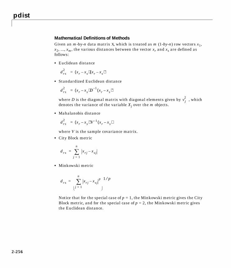
pdist
2-256
Mathematical Definitions of MethodsGiven an m-by-n data matrix X, which is treated as m (1-by-n) row vectors x1,x2, ..., xm, the various distances between the vector xr and xs are defined asfollows:
• Euclidean distance
• Standardized Euclidean distance
where D is the diagonal matrix with diagonal elements given by , whichdenotes the variance of the variable Xj over the m objects.
• Mahalanobis distance
where V is the sample covariance matrix.
• City Block metric
• Minkowski metric
Notice that for the special case of p = 1, the Minkowski metric gives the CityBlock metric, and for the special case of p = 2, the Minkowski metric givesthe Euclidean distance.
drs2 xr xs–( ) xr xs–( )'=
drs2 xr xs–( )D 1– xr xs–( )'=
vj2
drs2 xr xs–( )'V 1– xr xs–( )=
drs xrj xsj–j 1=
n
�=
drs xrj xsj–p
j 1=
n
�� � � �
1 p⁄=

pdist
2-257
Examples X = [1 2; 1 3; 2 2; 3 1]
X = 1 2 1 3 2 2 3 1
Y = pdist(X,'mahal')Y = 2.3452 2.0000 2.3452 1.2247 2.4495 1.2247
Y = pdist(X)Y = 1.0000 1.0000 2.2361 1.4142 2.8284 1.4142
squareform(Y)
ans = 0 1.0000 1.0000 2.2361 1.0000 0 1.4142 2.8284 1.0000 1.4142 0 1.4142 2.2361 2.8284 1.4142 0
See Also cluster, clusterdata, cophenet, dendrogram, inconsistent, linkage,squareform

perms
2-258
2permsPurpose All permutations.
Syntax P = perms(v)
Description P = perms(v) where v is a row vector of length n, creates a matrix whose rowsconsist of all possible permutations of the n elements of v. The matrix Pcontains n! rows and n columns.
perms is only practical when n is less than 8 or 9.
Example perms([2 4 6])
ans =
6 4 2 4 6 2 6 2 4 2 6 4 4 2 6 2 4 6

poisscdf
2-259
2poisscdfPurpose Poisson cumulative distribution function (cdf).
Syntax P = poisscdf(X,LAMBDA)
Description poisscdf(X,LAMBDA) computes the Poisson cdf at each of the values in X usingthe corresponding parameters in LAMBDA. Vector or matrix inputs for X andLAMBDA must be the same size. A scalar input is expanded to a constant matrixwith the same dimensions as the other input. The parameters in LAMBDA mustbe positive.
The Poisson cdf is
Examples For example, consider a Quality Assurance department that performs randomtests of individual hard disks. Their policy is to shut down the manufacturingprocess if an inspector finds more than four bad sectors on a disk. What is theprobability of shutting down the process if the mean number of bad sectors (λ)is two?
probability = 1 - poisscdf(4,2)
probability =
0.0527
About 5% of the time, a normally functioning manufacturing process willproduce more than four flaws on a hard disk.
Suppose the average number of flaws (λ) increases to four. What is theprobability of finding fewer than five flaws on a hard drive?
probability = poisscdf(4,4)
probability =
0.6288
This means that this faulty manufacturing process continues to operate afterthis first inspection almost 63% of the time.
p F x λ( ) e λ– λi
i!-----
i 0=
floor x( )
�= =

poisscdf
2-260
See Also cdf, poissfit, poissinv, poisspdf, poissrnd, poisstat
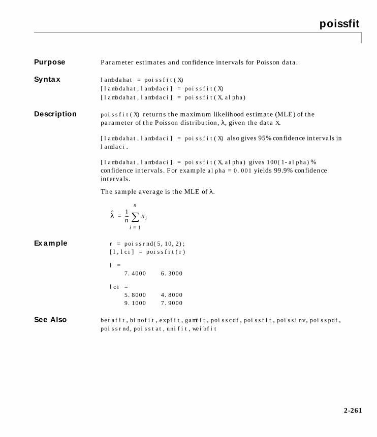
poissfit
2-261
2poissfitPurpose Parameter estimates and confidence intervals for Poisson data.
Syntax lambdahat = poissfit(X)[lambdahat,lambdaci] = poissfit(X)[lambdahat,lambdaci] = poissfit(X,alpha)
Description poissfit(X) returns the maximum likelihood estimate (MLE) of theparameter of the Poisson distribution, λ, given the data X.
[lambdahat,lambdaci] = poissfit(X) also gives 95% confidence intervals inlamdaci.
[lambdahat,lambdaci] = poissfit(X,alpha) gives 100(1-alpha)%confidence intervals. For example alpha = 0.001 yields 99.9% confidenceintervals.
The sample average is the MLE of λ.
Example r = poissrnd(5,10,2);[l,lci] = poissfit(r)
l =7.4000 6.3000
lci =5.8000 4.80009.1000 7.9000
See Also betafit, binofit, expfit, gamfit, poisscdf, poissfit, poissinv, poisspdf,poissrnd, poisstat, unifit, weibfit
λ 1n--- xi
i 1=
n
�=

poissinv
2-262
2poissinvPurpose Inverse of the Poisson cumulative distribution function (cdf).
Syntax X = poissinv(P,LAMBDA)
Description poissinv(P,LAMBDA) returns the smallest value X such that the Poisson cdfevaluated at X equals or exceeds P.
Examples If the average number of defects (λ) is two, what is the 95th percentile of thenumber of defects?
poissinv(0.95,2)
ans =
5
What is the median number of defects?
median_defects = poissinv(0.50,2)
median_defects =
2
See Also icdf, poisscdf, poissfit, poisspdf, poissrnd, poisstat

poisspdf
2-263
2poisspdfPurpose Poisson probability density function (pdf).
Syntax Y = poisspdf(X,LAMBDA)
Description poisspdf(X,LAMBDA) computes the Poisson pdf at each of the values in X usingthe corresponding parameters in LAMBDA. Vector or matrix inputs for X andLAMBDA must be the same size. A scalar input is expanded to a constant matrixwith the same dimensions as the other input. The parameters in LAMBDA mustall be positive.
The Poisson pdf is
where x can be any nonnegative integer. The density function is zero unless xis an integer.
Examples A computer hard disk manufacturer has observed that flaws occur randomly inthe manufacturing process at the average rate of two flaws in a 4 Gb hard diskand has found this rate to be acceptable. What is the probability that a disk willbe manufactured with no defects?
In this problem, λ = 2 and x = 0.
p = poisspdf(0,2)
p = 0.1353
See Also pdf, poisscdf, poissfit, poissinv, poissrnd, poisstat
y f x λ( ) λx
x!-----e λ– I 0 1 …, ,( ) x( )= =

poissrnd
2-264
2poissrndPurpose Random numbers from the Poisson distribution.
Syntax R = poissrnd(LAMBDA)R = poissrnd(LAMBDA,m)R = poissrnd(LAMBDA,m,n)
Description R = poissrnd(LAMBDA) generates Poisson random numbers with meanLAMBDA. The size of R is the size of LAMBDA.
R = poissrnd(LAMBDA,m) generates Poisson random numbers with meanLAMBDA, where m is a 1-by-2 vector that contains the row and columndimensions of R.
R = poissrnd(LAMBDA,m,n) generates Poisson random numbers with meanLAMBDA, where scalars m and n are the row and column dimensions of R.
Examples Generate a random sample of 10 pseudo-observations from a Poissondistribution with λ = 2.
lambda = 2;
random_sample1 = poissrnd(lambda,1,10)random_sample1 =
1 0 1 2 1 3 4 2 0 0
random_sample2 = poissrnd(lambda,[1 10])random_sample2 =
1 1 1 5 0 3 2 2 3 4
random_sample3 = poissrnd(lambda(ones(1,10)))random_sample3 =
3 2 1 1 0 0 4 0 2 0
See Also poisscdf, poissfit, poissinv, poisspdf, poisstat
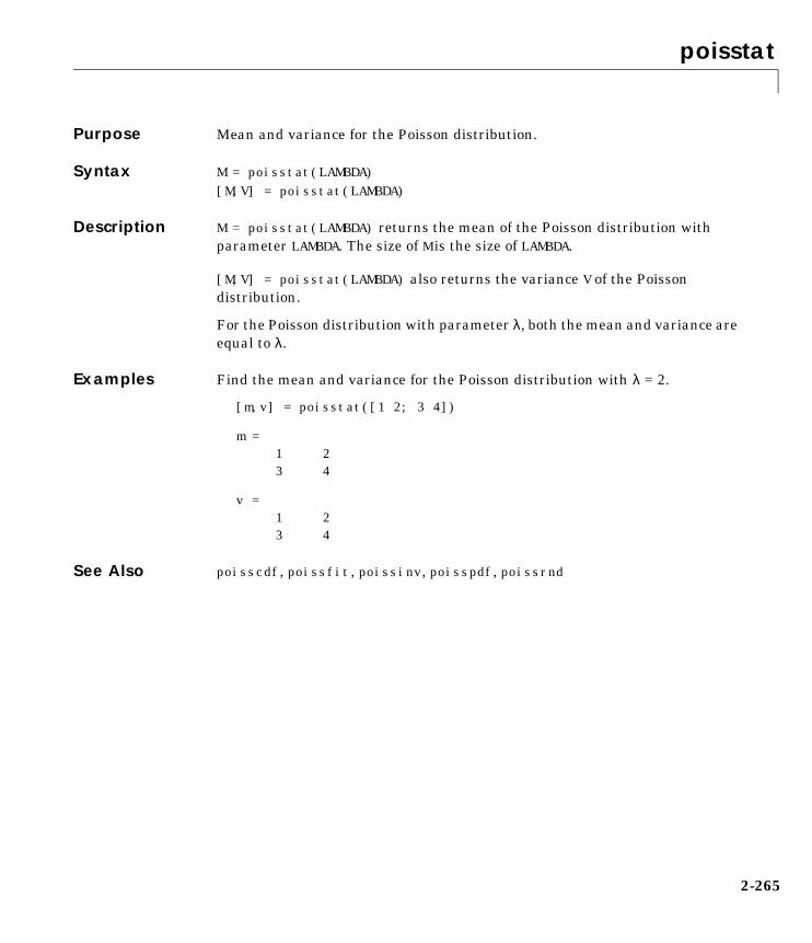
poisstat
2-265
2poisstatPurpose Mean and variance for the Poisson distribution.
Syntax M = poisstat(LAMBDA)[M,V] = poisstat(LAMBDA)
Description M = poisstat(LAMBDA) returns the mean of the Poisson distribution withparameter LAMBDA. The size of M is the size of LAMBDA.
[M,V] = poisstat(LAMBDA) also returns the variance V of the Poissondistribution.
For the Poisson distribution with parameter λ, both the mean and variance areequal to λ.
Examples Find the mean and variance for the Poisson distribution with λ = 2.
[m,v] = poisstat([1 2; 3 4])
m = 1 2 3 4
v = 1 2 3 4
See Also poisscdf, poissfit, poissinv, poisspdf, poissrnd
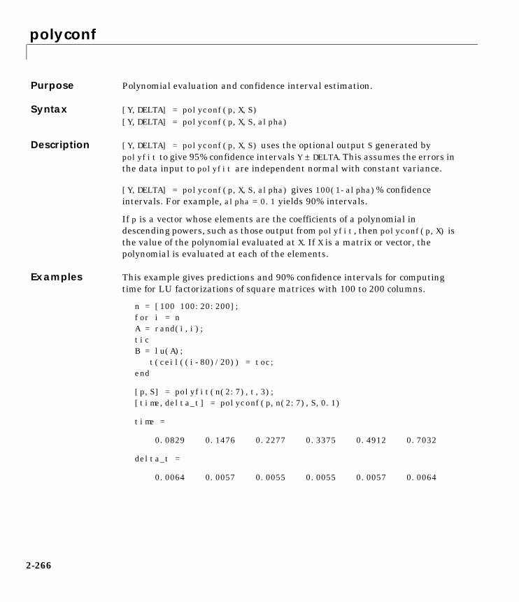
polyconf
2-266
2polyconfPurpose Polynomial evaluation and confidence interval estimation.
Syntax [Y,DELTA] = polyconf(p,X,S)[Y,DELTA] = polyconf(p,X,S,alpha)
Description [Y,DELTA] = polyconf(p,X,S) uses the optional output S generated bypolyfit to give 95% confidence intervals Y ± DELTA. This assumes the errors inthe data input to polyfit are independent normal with constant variance.
[Y,DELTA] = polyconf(p,X,S,alpha) gives 100(1-alpha)% confidenceintervals. For example, alpha = 0.1 yields 90% intervals.
If p is a vector whose elements are the coefficients of a polynomial indescending powers, such as those output from polyfit, then polyconf(p,X) isthe value of the polynomial evaluated at X. If X is a matrix or vector, thepolynomial is evaluated at each of the elements.
Examples This example gives predictions and 90% confidence intervals for computingtime for LU factorizations of square matrices with 100 to 200 columns.
n = [100 100:20:200];for i = nA = rand(i,i);ticB = lu(A);
t(ceil((i-80)/20)) = toc;end
[p,S] = polyfit(n(2:7),t,3);[time,delta_t] = polyconf(p,n(2:7),S,0.1)
time =
0.0829 0.1476 0.2277 0.3375 0.4912 0.7032
delta_t =
0.0064 0.0057 0.0055 0.0055 0.0057 0.0064

polyfit
2-267
2polyfitPurpose Polynomial curve fitting.
Syntax [p,S] = polyfit(x,y,n)
Description p = polyfit(x,y,n) finds the coefficients of a polynomial p(x) of degree nthat fits the data, p(x(i)) to y(i), in a least-squares sense. The result p is arow vector of length n+1 containing the polynomial coefficients in descendingpowers.
[p,S] = polyfit(x,y,n) returns polynomial coefficients p and matrix S foruse with polyval to produce error estimates on predictions. If the errors in thedata, y, are independent normal with constant variance, polyval will produceerror bounds which contain at least 50% of the predictions.
You may omit S if you are not going to pass it to polyval or polyconf forcalculating error estimates.
The polyfit function is part of the standard MATLAB language.
Example [p,S] = polyfit(1:10,[1:10] + normrnd(0,1,1,10),1)
p =
1.0300 0.4561
S =
-19.6214 -2.8031 0 -1.4639 8.0000 0 2.3180 0
See Also polyval, polytool, polyconf
p x( ) p1xn p2xn 1– … pnx pn 1++ + + +=

polytool
2-268
2polytoolPurpose Interactive plot for prediction of fitted polynomials.
Syntax polytool(x,y)polytool(x,y,n)polytool(x,y,n,alpha)
Description polytool(x,y) fits a line to the column vectors x and y and displays aninteractive plot of the result. This plot is graphic user interface for exploringthe effects of changing the polynomial degree of the fit. The plot shows thefitted curve and 95% global confidence intervals on a new predicted value forthe curve. Text with current predicted value of y and its uncertainty appears tothe left of the y-axis.
polytool(x,y,n) initially fits a polynomial of order n.
polytool(x,y,n,alpha) plots 100(1-alpha)% confidence intervals on thepredicted values.
polytool fits by least-squares using the regression model
Evaluate the function by typing a value in the x-axis edit box or by draggingthe vertical reference line on the plot. The shape of the pointer changes froman arrow to a cross hair when you are over the vertical line to indicate that theline can be dragged. The predicted value of y will update as you drag thereference line.
The argument n controls the degree of the polynomial fit. To change the degreeof the polynomial, choose from the pop-up menu at the top of the figure. Tochange the type of confidence intervals, use the Bounds menu. To change fromleast squares to a robust fitting method, use the Method menu.
When you are done, press the Close button.
yi β0 β1xi β2xi2 … βnxi
n εi+ + ++ +=
εi N 0 σ2,( )∼ i∀
Cov εi εj,( ) 0= i j,∀

polyval
2-269
2polyvalPurpose Polynomial evaluation.
Syntax Y = polyval(p,X)[Y,DELTA] = polyval(p,X,S)
Description Y = polyval(p,X) returns the predicted value of a polynomial given itscoefficients, p, at the values in X.
[Y,DELTA] = polyval(p,X,S) uses the optional output S generated bypolyfit to generate error estimates, Y ± DELTA. If the errors in the data inputto polyfit are independent normal with constant variance, Y ± DELTA containsat least 50% of the predictions.
If p is a vector whose elements are the coefficients of a polynomial indescending powers, then polyval(p,X) is the value of the polynomialevaluated at X. If X is a matrix or vector, the polynomial is evaluated at each ofthe elements.
The polyval function is part of the standard MATLAB language.
Examples Simulate the function y = x, adding normal random errors with a standarddeviation of 0.1. Then use polyfit to estimate the polynomial coefficients. Notethat predicted Y values are within DELTA of the integer X in every case.
[p,S] = polyfit(1:10,(1:10) + normrnd(0,0.1,1,10),1);X = magic(3);[Y,D] = polyval(p,X,S)
Y = 8.0696 1.0486 6.0636 3.0546 5.0606 7.0666 4.0576 9.0726 2.0516
D = 0.0889 0.0951 0.0861 0.0889 0.0861 0.0870 0.0870 0.0916 0.0916
See Also polyfit, polytool, polyconf
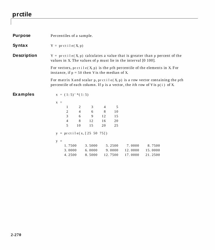
prctile
2-270
2prctilePurpose Percentiles of a sample.
Syntax Y = prctile(X,p)
Description Y = prctile(X,p) calculates a value that is greater than p percent of thevalues in X. The values of p must lie in the interval [0 100].
For vectors, prctile(X,p) is the pth percentile of the elements in X. Forinstance, if p = 50 then Y is the median of X.
For matrix X and scalar p, prctile(X,p) is a row vector containing the pthpercentile of each column. If p is a vector, the ith row of Y is p(i) of X.
Examples x = (1:5)'*(1:5)
x = 1 2 3 4 5 2 4 6 8 10 3 6 9 12 15 4 8 12 16 20 5 10 15 20 25
y = prctile(x,[25 50 75])
y = 1.7500 3.5000 5.2500 7.0000 8.7500 3.0000 6.0000 9.0000 12.0000 15.0000 4.2500 8.5000 12.7500 17.0000 21.2500

princomp
2-271
2princompPurpose Principal Components Analysis (PCA).
Syntax PC = princomp(X)[PC,SCORE,latent,tsquare] = princomp(X)
Description [PC,SCORE,latent,tsquare] = princomp(X) takes a data matrix X andreturns the principal components in PC, the so-called Z-scores in SCORE, theeigenvalues of the covariance matrix of X in latent, and Hotelling’s T2 statisticfor each data point in tsquare.
The Z-scores are the data formed by transforming the original data into thespace of the principal components. The values of the vector, latent, are thevariance of the columns of SCORE. Hotelling’s T2 is a measure of themultivariate distance of each observation from the center of the data set.
Example Compute principal components for the ingredients data in the Hald dataset,and the variance accounted for by each component.
load hald;[pc,score,latent,tsquare] = princomp(ingredients);pc,latent
pc = 0.0678 -0.6460 0.5673 -0.5062 0.6785 -0.0200 -0.5440 -0.4933 -0.0290 0.7553 0.4036 -0.5156 -0.7309 -0.1085 -0.4684 -0.4844
latent =
517.7969 67.4964 12.4054 0.2372
Reference Jackson, J. E., A User's Guide to Principal Components, John Wiley and Sons,Inc. 1991. pp. 1–25.
See Also barttest, pcacov, pcares

qqplot
2-272
2qqplotPurpose Quantile-quantile plot of two samples.
Syntax qqplot(X)qqplot(X,Y)qqplot(X,Y,pvec)h = qqplot(...)
Description qqplot(X) displays a quantile-quantile plot of the sample quantiles of X versustheoretical quantiles from a normal distribution. If the distribution of X isnormal, the plot will be close to linear.
qqplot(X,Y) displays a quantile-quantile plot of two samples. If the samplesdo come from the same distribution, the plot will be linear.
For matrix X and Y, qqplot displays a separate line for each pair of columns.The plotted quantiles are the quantiles of the smaller dataset.
The plot has the sample data displayed with the plot symbol '+'.Superimposed on the plot is a line joining the first and third quartiles of eachdistribution (this is a robust linear fit of the order statistics of the two samples).This line is extrapolated out to the ends of the sample to help evaluate thelinearity of the data.
Use qqplot(X,Y,pvec) to specify the quantiles in the vector pvec.
h = qqplot(X,Y,pvec) returns handles to the lines in h.
Examples Generate two normal samples with different means and standard deviations.Then make a quantile-quantile plot of the two samples.
x = normrnd(0,1,100,1);y = normrnd(0.5,2,50,1);qqplot(x,y);

qqplot
2-273
See Also normplot
-3 -2 -1 0 1 2 3-10
-5
0
5
10
X Quantiles
Y Q
uant
iles

random
2-274
2randomPurpose Random numbers from a specified distribution.
Syntax y = random('name',A1,A2,A3,m,n)
Description y = random('name',A1,A2,A3,m,n) returns a matrix of random numbers,where 'name' is a string containing the name of the distribution, and A1, A2,and A3 are matrices of distribution parameters. Depending on the distributionsome of the parameters may not be necessary.
Vector or matrix inputs must all have the same size. A scalar input is expandedto a constant matrix with the same dimensions as the other inputs.
The last two parameters, d and e, are the size of the matrix y. If thedistribution parameters are matrices, then these parameters are optional, butthey must match the size of the other matrix arguments (see second example).
random is a utility routine allowing you to access all the random numbergenerators in the Statistics Toolbox using the name of the distribution as aparameter. See “Overview of the Distributions” on page 1-12 for the list ofavailable distributions.
Examples rn = random('Normal',0,1,2,4)
rn = 1.1650 0.0751 -0.6965 0.0591 0.6268 0.3516 1.6961 1.7971
rp = random('Poisson',1:6,1,6)
rp = 0 0 1 2 5 7
See Also betarnd, binornd, cdf, chi2rnd, exprnd, frnd, gamrnd, geornd, hygernd, icdf,lognrnd, nbinrnd, ncfrnd, nctrnd, ncx2rnd, normrnd, pdf, poissrnd, raylrnd,trnd, unidrnd, unifrnd, weibrnd
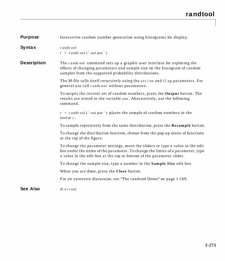
randtool
2-275
2randtoolPurpose Interactive random number generation using histograms for display.
Syntax randtoolr = randtool('output')
Description The randtool command sets up a graphic user interface for exploring theeffects of changing parameters and sample size on the histogram of randomsamples from the supported probability distributions.
The M-file calls itself recursively using the action and flag parameters. Forgeneral use call randtool without parameters.
To output the current set of random numbers, press the Output button. Theresults are stored in the variable ans. Alternatively, use the followingcommand.
r = randtool('output') places the sample of random numbers in thevector r.
To sample repetitively from the same distribution, press the Resample button.
To change the distribution function, choose from the pop-up menu of functionsat the top of the figure.
To change the parameter settings, move the sliders or type a value in the editbox under the name of the parameter. To change the limits of a parameter, typea value in the edit box at the top or bottom of the parameter slider.
To change the sample size, type a number in the Sample Size edit box.
When you are done, press the Close button.
For an extensive discussion, see “The randtool Demo” on page 1-169.
See Also disttool

range
2-276
2rangePurpose Sample range.
Syntax y = range(X)
Description range(X) returns the difference between the maximum and the minimum of asample. For vectors, range(x) is the range of the elements. For matrices,range(X) is a row vector containing the range of each column of X.
The range is an easily calculated estimate of the spread of a sample. Outliershave an undue influence on this statistic, which makes it an unreliableestimator.
Example The range of a large sample of standard normal random numbers isapproximately six. This is the motivation for the process capability indices Cpand Cpk in statistical quality control applications.
rv = normrnd(0,1,1000,5);near6 = range(rv)
near6 =
6.1451 6.4986 6.2909 5.8894 7.0002
See Also std, iqr, mad
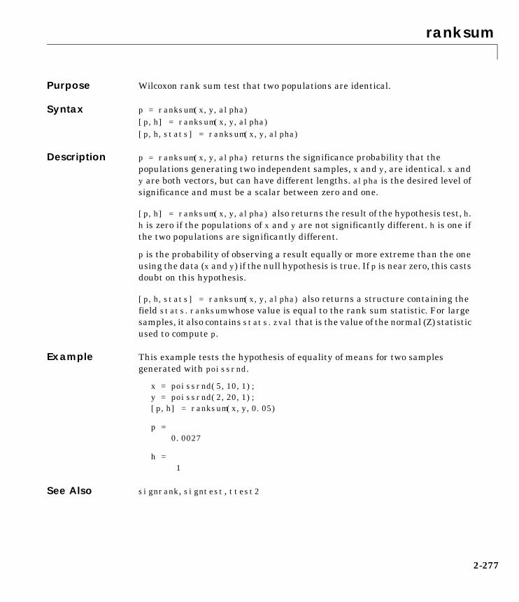
ranksum
2-277
2ranksumPurpose Wilcoxon rank sum test that two populations are identical.
Syntax p = ranksum(x,y,alpha)[p,h] = ranksum(x,y,alpha)[p,h,stats] = ranksum(x,y,alpha)
Description p = ranksum(x,y,alpha) returns the significance probability that thepopulations generating two independent samples, x and y, are identical. x andy are both vectors, but can have different lengths. alpha is the desired level ofsignificance and must be a scalar between zero and one.
[p,h] = ranksum(x,y,alpha) also returns the result of the hypothesis test, h.h is zero if the populations of x and y are not significantly different. h is one ifthe two populations are significantly different.
p is the probability of observing a result equally or more extreme than the oneusing the data (x and y) if the null hypothesis is true. If p is near zero, this castsdoubt on this hypothesis.
[p,h,stats] = ranksum(x,y,alpha) also returns a structure containing thefield stats.ranksum whose value is equal to the rank sum statistic. For largesamples, it also contains stats.zval that is the value of the normal (Z) statisticused to compute p.
Example This example tests the hypothesis of equality of means for two samplesgenerated with poissrnd.
x = poissrnd(5,10,1);y = poissrnd(2,20,1);[p,h] = ranksum(x,y,0.05)
p = 0.0027
h = 1
See Also signrank, signtest, ttest2

raylcdf
2-278
2raylcdfPurpose Rayleigh cumulative distribution function (cdf).
Syntax P = raylcdf(X,B)
Description P = raylcdf(X,B) computes the Rayleigh cdf at each of the values in X usingthe corresponding parameters in B. Vector or matrix inputs for X and B musthave the same size, which is also the size of P. A scalar input for X or B isexpanded to a constant matrix with the same dimensions as the other input.
The Rayleigh cdf is
Example x = 0:0.1:3;p = raylcdf(x,1);plot(x,p)
Reference Evans, M., N. Hastings, and B. Peacock, Statistical Distributions, SecondEdition, Wiley 1993. pp. 134–136.
See Also cdf, raylinv, raylpdf, raylrnd, raylstat
y F x b( ) t
b2------
0
x
� e
t2–
2b2---------� �� �
= = dt
0 0.5 1 1.5 2 2.5 30
0.2
0.4
0.6
0.8
1

raylinv
2-279
2raylinvPurpose Inverse of the Rayleigh cumulative distribution function.
Syntax X = raylinv(P,B)
Description X = raylinv(P,B) returns the inverse of the Rayleigh cumulative distributionfunction with parameter B at the corresponding probabilities in P. Vector ormatrix inputs for P and B must have the same size, which is also the size of X.A scalar input for P or B is expanded to a constant matrix with the samedimensions as the other input.
Example x = raylinv(0.9,1)
x = 2.1460
See Also icdf, raylcdf, raylpdf, raylrnd, raylstat

raylpdf
2-280
2raylpdfPurpose Rayleigh probability density function.
Syntax Y = raylpdf(X,B)
Description Y = raylpdf(X,B) computes the Rayleigh pdf at each of the values in X usingthe corresponding parameters in B. Vector or matrix inputs for X and B musthave the same size, which is also the size of Y. A scalar input for X or B isexpanded to a constant matrix with the same dimensions as the other input.
The Rayleigh pdf is
Example x = 0:0.1:3;p = raylpdf(x,1);plot(x,p)
See Also pdf, raylcdf, raylinv, raylrnd, raylstat
y f x b( ) x
b2------e
x2–
2b2---------� �� �
= =
0 0.5 1 1.5 2 2.5 30
0.2
0.4
0.6
0.8
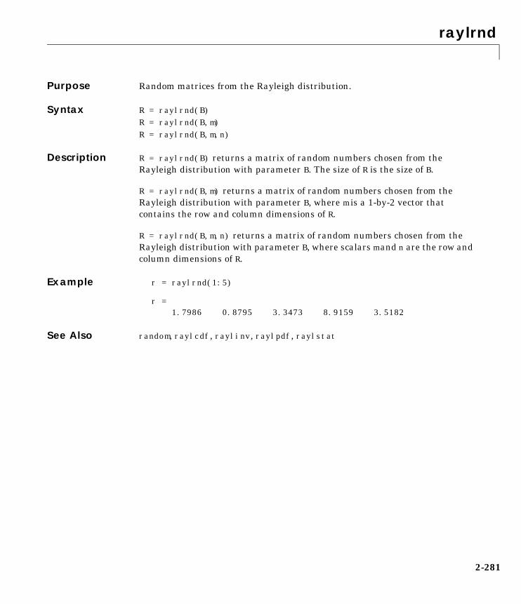
raylrnd
2-281
2raylrndPurpose Random matrices from the Rayleigh distribution.
Syntax R = raylrnd(B)R = raylrnd(B,m)R = raylrnd(B,m,n)
Description R = raylrnd(B) returns a matrix of random numbers chosen from theRayleigh distribution with parameter B. The size of R is the size of B.
R = raylrnd(B,m) returns a matrix of random numbers chosen from theRayleigh distribution with parameter B, where m is a 1-by-2 vector thatcontains the row and column dimensions of R.
R = raylrnd(B,m,n) returns a matrix of random numbers chosen from theRayleigh distribution with parameter B, where scalars m and n are the row andcolumn dimensions of R.
Example r = raylrnd(1:5)
r = 1.7986 0.8795 3.3473 8.9159 3.5182
See Also random, raylcdf, raylinv, raylpdf, raylstat

raylstat
2-282
2raylstatPurpose Mean and variance for the Rayleigh distribution.
Syntax M = raylstat(B)[M,V] = raylstat(B)
Description [M,V] = raylstat(B) returns the mean and variance of the Rayleighdistribution with parameter B.
The mean of the Rayleigh distribution with parameter b is and thevariance is
Example [mn,v] = raylstat(1)
mn = 1.2533
v = 0.4292
See Also raylcdf, raylinv, raylpdf, raylrnd
b π 2⁄
4 π–2
------------b2

rcoplot
2-283
2rcoplotPurpose Residual case order plot.
Syntax rcoplot(r,rint)
Description rcoplot(r,rint) displays an errorbar plot of the confidence intervals on theresiduals from a regression. The residuals appear in the plot in case order.Inputs r and rint are outputs from the regress function.
Example X = [ones(10,1) (1:10)'];y = X ∗ [10;1] + normrnd(0,0.1,10,1);[b,bint,r,rint] = regress(y,X,0.05);rcoplot(r,rint);
The figure shows a plot of the residuals with error bars showing 95% confidenceintervals on the residuals. All the error bars pass through the zero line,indicating that there are no outliers in the data.
See Also regress
0 2 4 6 8 10
-0.2
-0.1
0
0.1
0.2
Res
idua
ls
Case Number

refcurve
2-284
2refcurvePurpose Add a polynomial curve to the current plot.
Syntax h = refcurve(p)
Description refcurve adds a graph of the polynomial p to the current axes. The function fora polynomial of degree n is:
y = p1xn + p2x(n-1) + ... + pnx + pn+1
Note that p1 goes with the highest order term.
h = refcurve(p) returns the handle to the curve.
Example Plot data for the height of a rocket against time, and add a reference curveshowing the theoretical height (assuming no air friction). The initial velocity ofthe rocket is 100 m/sec.
h = [85 162 230 289 339 381 413 437 452 458 456 440 400 356];plot(h,'+')refcurve([-4.9 100 0])
See Also polyfit, polyval, refline
0 2 4 6 8 10 12 140
100
200
300
400
500

refline
2-285
2reflinePurpose Add a reference line to the current axes.
Syntax refline(slope,intercept)refline(slope)h = refline(slope,intercept)refline
Description refline(slope,intercept) adds a reference line with the given slope andintercept to the current axes.
refline(slope), where slope is a two-element vector, adds the line
y = slope(2) + slope(1)*x
to the figure.
h = refline(slope,intercept) returns the handle to the line.
refline with no input arguments superimposes the least squares line on eachline object in the current figure (except LineStyles '-','--','.-'). Thisbehavior is equivalent to lsline.
Example y = [3.2 2.6 3.1 3.4 2.4 2.9 3.0 3.3 3.2 2.1 2.6]';plot(y,'+')refline(0,3)
See Also lsline, polyfit, polyval, refcurve
0 2 4 6 8 10 122
2.5
3
3.5
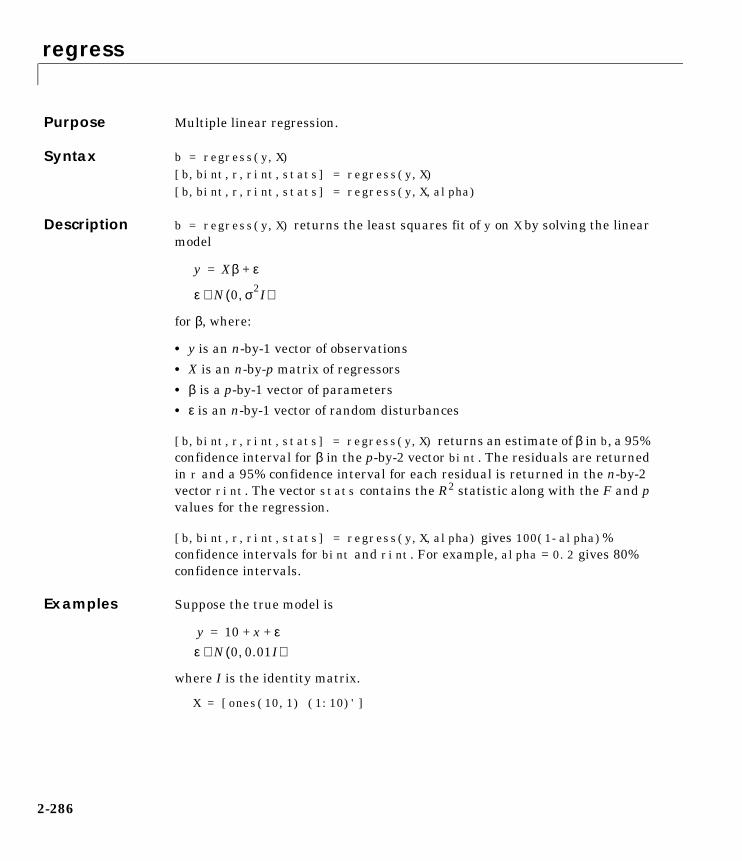
regress
2-286
2regressPurpose Multiple linear regression.
Syntax b = regress(y,X)[b,bint,r,rint,stats] = regress(y,X)[b,bint,r,rint,stats] = regress(y,X,alpha)
Description b = regress(y,X) returns the least squares fit of y on X by solving the linearmodel
for β, where:
• y is an n-by-1 vector of observations
• X is an n-by-p matrix of regressors
• β is a p-by-1 vector of parameters
• ε is an n-by-1 vector of random disturbances
[b,bint,r,rint,stats] = regress(y,X) returns an estimate of β in b, a 95%confidence interval for β in the p-by-2 vector bint. The residuals are returnedin r and a 95% confidence interval for each residual is returned in the n-by-2vector rint. The vector stats contains the R2 statistic along with the F and pvalues for the regression.
[b,bint,r,rint,stats] = regress(y,X,alpha) gives 100(1-alpha)%confidence intervals for bint and rint. For example, alpha = 0.2 gives 80%confidence intervals.
Examples Suppose the true model is
where I is the identity matrix.
X = [ones(10,1) (1:10)']
y Xβ ε+=
ε N 0 σ2I,( )∼
y 10 x ε+ +=
ε N 0 0.01I,( )∼
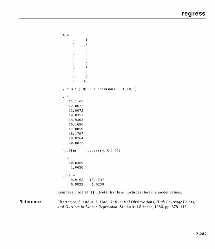
regress
2-287
X = 1 1 1 2 1 3 1 4 1 5 1 6 1 7 1 8 1 9 1 10
y = X ∗ [10;1] + normrnd(0,0.1,10,1)
y = 11.1165 12.0627 13.0075 14.0352 14.9303 16.1696 17.0059 18.1797 19.0264 20.0872
[b,bint] = regress(y,X,0.05)
b = 10.0456 1.0030
bint = 9.9165 10.1747 0.9822 1.0238
Compare b to [10 1]'. Note that bint includes the true model values.
Reference Chatterjee, S. and A. S. Hadi. Influential Observations, High Leverage Points,and Outliers in Linear Regression. Statistical Science, 1986. pp. 379–416.

regstats
2-288
2regstatsPurpose Regression diagnostics graphical user interface.
Syntax regstats(responses,DATA)regstats(responses,DATA,'model')
Description regstats(responses,DATA) generates regression diagnostics for a linearadditive model with a constant term. The dependent variable is the vectorresponses. Values of the independent variables are in the matrix DATA.
The function creates a figure with a group of check boxes that save diagnosticstatistics to the base workspace using variable names you can specify.
regstats(responses,data,'model') controls the order of the regressionmodel, where 'model' can be one of these strings:
• 'interaction' – includes constant, linear, and cross product terms
• 'quadratic' – includes interactions and squared terms
• 'purequadratic' – includes constant, linear, and squared terms
The literature suggests many diagnostic statistics for evaluating multiplelinear regression. regstats provides these diagnostics:
• Q from QR decomposition
• R from QR decomposition
• Regression coefficients
• Covariance of regression coefficients
• Fitted values of the response data
• Residuals
• Mean squared error
• Leverage
• “Hat” matrix
• Delete-1 variance
• Delete-1 coefficients
• Standardized residuals
• Studentized residuals
• Change in regression coefficients

regstats
2-289
• Change in fitted values
• Scaled change in fitted values
• Change in covariance
• Cook's distance
For more detail press the Help button in the regstats window. This providesformulae and interpretations for each of these regression diagnostics.
Algorithm The usual regression model is y = Xβ + ε, where:
• y is an n-by-1 vector of responses
• X is an n-by-p matrix of predictors
• β is an p-by-1 vector of parameters
• ε is an n-by-1 vector of random disturbances
Let X = Q*R where Q and R come from a QR Decomposition of X. Q is orthogonaland R is triangular. Both of these matrices are useful for calculating manyregression diagnostics (Goodall 1993).
The standard textbook equation for the least squares estimator of β is
However, this definition has poor numeric properties. Particularly dubious isthe computation of , which is both expensive and imprecise.
Numerically stable MATLAB code for β is
b = R\(Q'*y);
Reference Goodall, C. R. (1993). Computation using the QR decomposition. Handbook inStatistics, Volume 9. Statistical Computing (C. R. Rao, ed.). Amsterdam, NLElsevier/North-Holland.
See Also leverage, stepwise, regress
β b X'X( ) 1– X'y= =
X'X( ) 1–
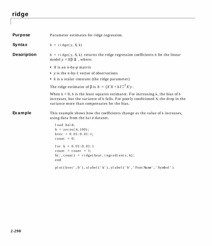
ridge
2-290
2ridgePurpose Parameter estimates for ridge regression.
Syntax b = ridge(y,X,k)
Description b = ridge(y,X,k) returns the ridge regression coefficients b for the linearmodel y = Xβ + ε, where:
• X is an n-by-p matrix
• y is the n-by-1 vector of observations
• k is a scalar constant (the ridge parameter)
The ridge estimator of β is .
When k = 0, b is the least squares estimator. For increasing k, the bias of bincreases, but the variance of b falls. For poorly conditioned X, the drop in thevariance more than compensates for the bias.
Example This example shows how the coefficients change as the value of k increases,using data from the hald dataset.
load hald;b = zeros(4,100);kvec = 0.01:0.01:1;count = 0;
for k = 0.01:0.01:1count = count + 1;b(:,count) = ridge(heat,ingredients,k);end
plot(kvec',b'),xlabel('k'),ylabel('b','FontName','Symbol')
b X'X kI+( ) 1– X'y=

ridge
2-291
See Also regress, stepwise
0 0.2 0.4 0.6 0.8 1-10
-5
0
5
10
k
β

robustdemo
2-292
2robustdemoPurpose Demo of robust regression.
Syntax robustdemorobustdemo(X,Y)
Description rsmdemo demonstrates robust regression and ordinary least squares regressionon a sample dataset. The function creates a figure window containing a scatterplot of sample data vectors X and Y, along with two fitted lines calculated usingleast squares and the robust bisquare method. The bottom of the figure showsthe equations of the lines and the estimated error standard deviations for eachfit. If you use the left mouse button to select an point and move it to a newlocation, both fits will update. If you hold down the right mouse button over anypoint, the point will be labeled with the leverage of that point on the leastsquares fit, and the weight of that point in the robust fit.
rsmdemo(X,Y) performs the same demonstration using the X and Y values thatyou specify.
Example See “The robustdemo Demo” on page 1-172.
See Also robustfit, leverage

robustfit
2-293
2robustfitPurpose Robust regression.
Syntax b = robustfit(X,Y)[b,stats] = robustfit(X,Y)[b,stats] = robustfit(X,Y,'wfun',tune,'const')
Description b = robustfit(X,Y) uses robust regression to fit Y as a function of thecolumns of X, and returns the vector b of coefficient estimates. The robustfitfunction uses an iteratively reweighted least squares algorithm, with theweights at each iteration calculated by applying the bisquare function to theresiduals from the previous iteration. This algorithm gives lower weight topoints that do not fit well. The results are less sensitive to outliers in the dataas compared with ordinary least squares regression.
[b,stats] = robustfit(X,Y) also returns a stats structure with thefollowing fields:
• stats.ols_s – sigma estimate (rmse) from least squares fit
• stats.robust_s – robust estimate of sigma
• stats.mad_s – estimate of sigma computed using the median absolutedeviation of the residuals from their median; used for scaling residualsduring the iterative fitting
• stats.s – final estimate of sigma, the larger of robust_s and a weightedaverage of ols_s and robust_s
• stats.se – standard error of coefficient estimates
• stats.t – ratio of b to stats.se
• stats.p – p-values for stats.t
• stats.coeffcorr – estimated correlation of coefficient estimates
• stats.w – vector of weights for robust fit
• stats.h – vector of leverage values for least squares fit
• stats.dfe – degrees of freedom for error
• stats.R – R factor in QR decomposition of X matrix
The robustfit function estimates the variance-covariance matrix of thecoefficient estimates as V = inv(X'*X)*stats.s^2. The standard errors andcorrelations are derived from V.

robustfit
2-294
[b,stats] = robustfit(X,Y,'wfun',tune,'const') specifies a weightfunction, a tuning constant, and the presence or absence of a constant term.The weight function 'wfun' can be any of the names listed in the followingtable.
The value r in the weight function expression is equal to
resid/(tune*s*sqrt(1-h))
where resid is the vector of residuals from the previous iteration, tune is thetuning constant, h is the vector of leverage values from a least squares fit, ands is an estimate of the standard deviation of the error term.
s = MAD/0.6745
The quantity MAD is the median absolute deviation of the residuals from theirmedian. The constant 0.6745 makes the estimate unbiased for the normaldistribution. If there are p columns in the X matrix (including the constantterm, if any), the smallest p-1 absolute deviations are excluded whencomputing their median.
In addition to the function names listed above, 'wfun' can be 'ols' to performunweighted ordinary least squares.
The argument tune overrides the default tuning constant from the table. Asmaller tuning constant tends to downweight large residuals more severely,
Weight function Meaning Tuning constant
'andrews' w = (abs(r)<pi) .* sin(r) ./ r 1.339
'bisquare' w = (abs(r)<1) .* (1 - r.^2).^2 4.685
'cauchy' w = 1 ./ (1 + r.^2) 2.385
'fair' w = 1 ./ (1 + abs(r)) 1.400
'huber' w = 1 ./ max(1, abs(r)) 1.345
'logistic' w = tanh(r) ./ r 1.205
'talwar' w = 1 * (abs(r)<1) 2.795
'welsch' w = exp(-(r.^2)) 2.985
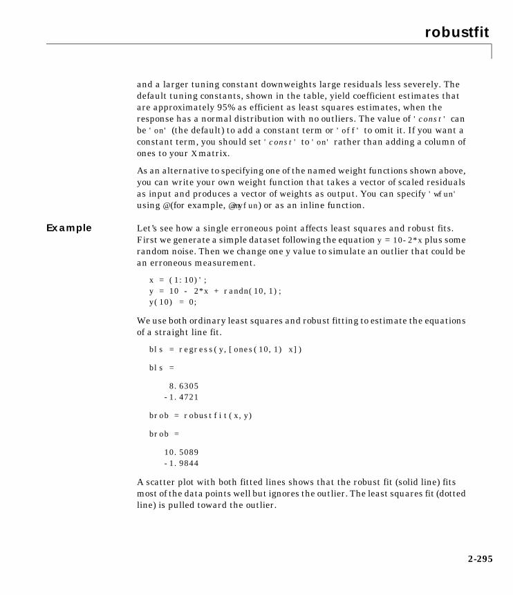
robustfit
2-295
and a larger tuning constant downweights large residuals less severely. Thedefault tuning constants, shown in the table, yield coefficient estimates thatare approximately 95% as efficient as least squares estimates, when theresponse has a normal distribution with no outliers. The value of 'const' canbe 'on' (the default) to add a constant term or 'off' to omit it. If you want aconstant term, you should set 'const' to 'on' rather than adding a column ofones to your X matrix.
As an alternative to specifying one of the named weight functions shown above,you can write your own weight function that takes a vector of scaled residualsas input and produces a vector of weights as output. You can specify 'wfun' using @ (for example, @myfun) or as an inline function.
Example Let’s see how a single erroneous point affects least squares and robust fits.First we generate a simple dataset following the equation y = 10-2*x plus somerandom noise. Then we change one y value to simulate an outlier that could bean erroneous measurement.
x = (1:10)';y = 10 - 2*x + randn(10,1);y(10) = 0;
We use both ordinary least squares and robust fitting to estimate the equationsof a straight line fit.
bls = regress(y,[ones(10,1) x])
bls =
8.6305 -1.4721
brob = robustfit(x,y)
brob =
10.5089 -1.9844
A scatter plot with both fitted lines shows that the robust fit (solid line) fitsmost of the data points well but ignores the outlier. The least squares fit (dottedline) is pulled toward the outlier.
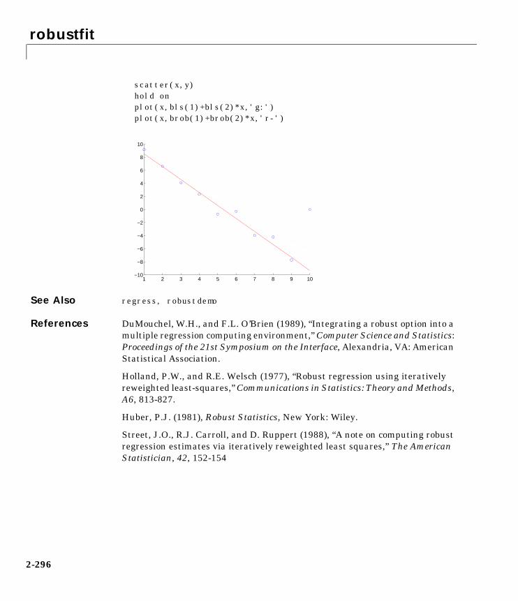
robustfit
2-296
scatter(x,y)hold onplot(x,bls(1)+bls(2)*x,'g:')plot(x,brob(1)+brob(2)*x,'r-')
See Also regress, robustdemo
References DuMouchel, W.H., and F.L. O’Brien (1989), “Integrating a robust option into amultiple regression computing environment,” Computer Science and Statistics:Proceedings of the 21st Symposium on the Interface, Alexandria, VA: AmericanStatistical Association.
Holland, P.W., and R.E. Welsch (1977), “Robust regression using iterativelyreweighted least-squares,” Communications in Statistics: Theory and Methods,A6, 813-827.
Huber, P.J. (1981), Robust Statistics, New York: Wiley.
Street, J.O., R.J. Carroll, and D. Ruppert (1988), “A note on computing robustregression estimates via iteratively reweighted least squares,” The AmericanStatistician, 42, 152-154
1 2 3 4 5 6 7 8 9 10−10
−8
−6
−4
−2
0
2
4
6
8
10

rowexch
2-297
2rowexchPurpose D-optimal design of experiments – row exchange algorithm.
Syntax settings = rowexch(nfactors,nruns)[settings,X] = rowexch(nfactors,nruns)[settings,X] = rowexch(nfactors,nruns,'model')
Description settings = rowexch(nfactors,nruns) generates the factor settings matrix,settings, for a D-Optimal design using a linear additive model with a constantterm. settings has nruns rows and nfactors columns.
[settings,X] = rowexch(nfactors,nruns) also generates the associateddesign matrix X.
[settings,X] = rowexch(nfactors,nruns,'model') produces a design forfitting a specified regression model. The input, 'model', can be one of thesestrings:
• 'interaction' – includes constant, linear, and cross product terms.
• 'quadratic' – interactions plus squared terms.
• 'purequadratic' – includes constant, linear and squared terms.
Example This example illustrates that the D-optimal design for three factors in eightruns, using an interactions model, is a two level full-factorial design.
s = rowexch(3,8,'interaction')
s = -1 -1 1 1 -1 -1 1 -1 1 -1 -1 -1 -1 1 1 1 1 1 -1 1 -1 1 1 -1
See Also cordexch, daugment, dcovary, fullfact, ff2n, hadamard

rsmdemo
2-298
2rsmdemoPurpose Demo of design of experiments and surface fitting.
Syntax rsmdemo
Description rsmdemo creates a GUI that simulates a chemical reaction. To start, you havea budget of 13 test reactions. Try to find out how changes in each reactant affectthe reaction rate. Determine the reactant settings that maximize the reactionrate. Estimate the run-to-run variability of the reaction. Now run a designedexperiment using the model pop-up. Compare your previous results with theoutput from response surface modeling or nonlinear modeling of the reaction.The GUI has the following elements:
• A Run button to perform one reactor run at the current settings
• An Export button to export the x and y data to the base workspace
• Three sliders with associated data entry boxes to control the partialpressures of the chemical reactants: Hydrogen, n-Pentane, and Isopentane
• A text box to report the reaction rate
• A text box to keep track of the number of test reactions you have left
Example See “The rsmdemo Demo” on page 1-170.
See Also rstool, nlintool, cordexch

rstool
2-299
2rstoolPurpose Interactive fitting and visualization of a response surface.
Syntax rstool(x,y)rstool(x,y,'model')rstool(x,y,'model',alpha,'xname','yname')
Description rstool(x,y) displays an interactive prediction plot with 95% global confidenceintervals. This plot results from a multiple regression of (x,y) data using alinear additive model.
rstool(x,y,'model') allows control over the initial regression model, where'model' can be one of the following strings:
• 'interaction' – includes constant, linear, and cross product terms
• 'quadratic' – includes interactions and squared terms
• 'purequadratic' – includes constant, linear and squared terms
rstool(x,y,'model',alpha) plots 100(1-alpha)% global confidence intervalfor predictions as two red curves. For example, alpha = 0.01 gives 99%confidence intervals.
rstool displays a “vector” of plots, one for each column of the matrix ofinputs x. The response variable, y, is a column vector that matches the numberof rows in x.
rstool(x,y,'model',alpha,'xname','yname') labels the graph using thestring matrix 'xname' for the labels to the x-axes and the string, 'yname', tolabel the y-axis common to all the plots.
Drag the dotted white reference line and watch the predicted values updatesimultaneously. Alternatively, you can get a specific prediction by typing thevalue of x into an editable text field. Use the pop-up menu labeled Model tointeractively change the model. Use the pop-up menu labeled Export to movespecified variables to the base workspace.
Example See “Quadratic Response Surface Models” on page 1-86.
See Also nlintool

schart
2-300
2schartPurpose Chart of standard deviation for Statistical Process Control.
Syntax schart(DATA,conf)schart(DATA,conf,specs)schart(DATA,conf,specs)[outliers,h] = schart(DATA,conf,specs)
Description schart(data) displays an S chart of the grouped responses in DATA. The rowsof DATA contain replicate observations taken at a given time. The rows must bein time order. The graph contains the sample standard deviation s for eachgroup, a center line at the average s value, and upper and lower control limits.The limits are placed at a three-sigma distance on either side of the center line,where sigma is an estimate of the standard deviation of s. If the process is incontrol, fewer than 3 out of 1000 observations would be expected to fall outsidethe control limits by random chance. So, if you observe points outside thelimits, you can take this as evidence that the process is not in control.
schart(DATA,conf) allows control of the confidence level of the upper andlower plotted control limits. The default conf = 0.9973 produces three-sigmalimits.
norminv(1 - (1-.9973)/2)ans = 3
To get k-sigma limits, use the expression 1-2*(1-normcdf(k)). For example,the correct conf value for 2-sigma limits is 0.9545, as shown below.
k = 2;1-2*(1-normcdf(k))ans = 0.9545
schart(DATA,conf,specs) plots the specification limits in the two elementvector specs.
[outliers,h] = schart(data,conf,specs) returns outliers, a vector ofindices to the rows where the mean of DATA is out of control, and h, a vector ofhandles to the plotted lines.

schart
2-301
Example This example plots an S chart of measurements on newly machined parts,taken at one hour intervals for 36 hours. Each row of the runout matrixcontains the measurements for 4 parts chosen at random. The values indicate,in thousandths of an inch, the amount the part radius differs from the targetradius.
load partsschart(runout)
All points are within the control limits, so the variability within subgroups isconsistent with what would be expected by random chance. There is noevidence that the process is out of control.
Reference Montgomery, D., Introduction to Statistical Quality Control, John Wiley andSons 1991. p. 235.
See Also capaplot, ewmaplot, histfit, xbarplot
0 5 10 15 20 25 30 35 400
0.05
0.1
0.15
0.2
0.25
0.3
0.35
UCL
LCL
CL
S Chart
Sample Number
Sta
ndar
d D
evia
tion

signrank
2-302
2signrankPurpose Wilcoxon signed rank test of equality of medians.
Syntax p = signrank(x,y,alpha)[p,h] = signrank(x,y,alpha)[p,h,stats] = signrank(x,y,alpha)
Description p = signrank(x,y,alpha) returns the significance probability that themedians of two matched samples, x and y, are equal. x and y must be vectorsof equal length. y may also be a scalar; in this case, signrank computes theprobability that the median of x is different from the constant y. alpha is thedesired level of significance, and must be a scalar between zero and one.
[p,h] = signrank(x,y,alpha) also returns the result of the hypothesistest, h. h is zero if the difference in medians of x and y is not significantlydifferent from zero. h is one if the two medians are significantly different.
p is the probability of observing a result equally or more extreme than the oneusing the data (x and y) if the null hypothesis is true. p is calculated using therank values for the differences between corresponding elements in x and y. If pis near zero, this casts doubt on this hypothesis.
[p,h,stats] = signrank(x,y,alpha) also returns a structure statscontaining the field stats.signedrank whose value is the signed rankstatistic. For large samples, it also contains stats.zval, the value of thenormal (Z) statistic used to compute p.
Example This example tests the hypothesis of equality of means for two samplesgenerated with normrnd. The samples have the same theoretical mean butdifferent standard deviations.
x = normrnd(0,1,20,1);y = normrnd(0,2,20,1);[p,h] = signrank(x,y,0.05)
p = 0.2959
h = 0

signrank
2-303
See Also ranksum, signtest, ttest

signtest
2-304
2signtestPurpose Sign test for paired samples.
Syntax p = signtest(x,y,alpha)[p,h] = signtest(x,y,alpha)[p,h,stats] = signtest(x,y,alpha)
Description p = signtest(x,y,alpha) returns the significance probability that themedians of two matched samples, x and y, are equal. x and y must be vectorsof equal length. y may also be a scalar; in this case, signtest computes theprobability that the median of x is different from the constant y. alpha is thedesired level of significance and must be a scalar between zero and one.
[p,h] = signtest(x,y,alpha) also returns the result of the hypothesis test,h. h is 0 if the difference in medians of x and y is not significantly different fromzero. h is 1 if the two medians are significantly different.
p is the probability of observing a result equally or more extreme than the oneusing the data (x and y) if the null hypothesis is true. p is calculated using thesigns (plus or minus) of the differences between corresponding elements in xand y. If p is near zero, this casts doubt on this hypothesis.
[p,h,stats] = signtest(x,y,alpha) also returns a structure statscontaining the field stats.sign whose value is the sign statistic. For largesamples, it also contains stats.zval, the value of the normal (Z) statistic usedto compute p.
Example This example tests the hypothesis of equality of medians for two samplesgenerated with normrnd. The samples have the same theoretical median butdifferent standard deviations. (For the normal distribution, the mean andmedian are the same.)
x = normrnd(0,1,20,1);y = normrnd(0,2,20,1);[p,h] = signtest(x,y,0.05)
p = 0.2632
h = 0

signtest
2-305
See Also ranksum, signrank, ttest

skewness
2-306
2skewnessPurpose Sample skewness.
Syntax y = skewness(X)y = skewness(X,flag)
Description y = skewness(X) returns the sample skewness of X. For vectors, skewness(x)is the skewness of the elements of x. For matrices, skewness(X) is a row vectorcontaining the sample skewness of each column.
Skewness is a measure of the asymmetry of the data around the sample mean.If skewness is negative, the data are spread out more to the left of the meanthan to the right. If skewness is positive, the data are spread out more to theright. The skewness of the normal distribution (or any perfectly symmetricdistribution) is zero.
The skewness of a distribution is defined as
where µ is the mean of x, σ is the standard deviation of x, and E(t) representsthe expected value of the quantity t.
y = skewness(X,flag) specifies whether to correct for bias (flag = 0) or not(flag = 1, the default). When X represents a sample from a population, theskewness of X is biased; that is, it will tend to differ from the populationskewness by a systematic amount that depends on the size of the sample. Youcan set flag = 0 to correct for this systematic bias.
Example X = randn([5 4])
X = 1.1650 1.6961 -1.4462 -0.3600 0.6268 0.0591 -0.7012 -0.1356 0.0751 1.7971 1.2460 -1.3493 0.3516 0.2641 -0.6390 -1.2704 -0.6965 0.8717 0.5774 0.9846
y E x µ–( )3
σ3------------------------=

skewness
2-307
y = skewness(X)
y = -0.2933 0.0482 0.2735 0.4641
See Also kurtosis, mean, moment, std, var

squareform
2-308
2squareform
Purpose Reformat the output of pdist into a square matrix.
Syntax S = squareform(Y)
Description S = squareform(Y) reformats the distance information returned by pdistfrom a vector into a square matrix. In this format, S(i,j) denotes the distancebetween the i and j observations in the original data.
See Also pdist

std
2-309
2stdPurpose Standard deviation of a sample.
Syntax y = std(X)
Description y = std(X) computes the sample standard deviation of the data in X. Forvectors, std(x) is the standard deviation of the elements in x. For matrices,std(X) is a row vector containing the standard deviation of each column of X.
std normalizes by n-1 where n is the sequence length. For normally distributeddata, the square of the standard deviation is the minimum variance unbiasedestimator of σ 2 (the second parameter).
The standard deviation is
where the sample average is .
The std function is part of the standard MATLAB language.
Examples In each column, the expected value of y is one.
x = normrnd(0,1,100,6);y = std(x)
y = 0.9536 1.0628 1.0860 0.9927 0.9605 1.0254
y = std(-1:2:1)
y = 1.4142
See Also cov, var
s 1n 1–------------- xi x–( )2
i 1=
n
�� �� �� �� �
12---
=
x 1n--- xi�=

stepwise
2-310
2stepwisePurpose Interactive environment for stepwise regression.
Syntax stepwise(X,y)stepwise(X,y,inmodel)stepwise(X,y,inmodel,alpha)
Description stepwise(X,y) fits a regression model of y on the columns of X. It displaysthree figure windows for interactively controlling the stepwise addition andremoval of model terms.
stepwise(X,y,inmodel) allows control of the terms in the original regressionmodel. The values of vector, inmodel, are the indices of the columns of thematrix X to include in the initial model.
stepwise(X,y,inmodel,alpha) allows control of the length confidenceintervals on the fitted coefficients. alpha is the significance for testing eachterm in the model. By default, alpha = 1 - (1 - 0.025)(1/p) where p is the numberof columns in X. This translates to plotted 95% simultaneous confidenceintervals (Bonferroni) for all the coefficients.
The least squares coefficient is plotted with a green filled circle. A coefficient isnot significantly different from zero if its confidence interval crosses the whitezero line. Significant model terms are plotted using solid lines. Terms notsignificantly different from zero are plotted with dotted lines.
Click on the confidence interval lines to toggle the state of the modelcoefficients. If the confidence interval line is green, the term is in the model. Ifthe confidence interval line is red, the term is not in the model.
Use the Export menu to move variables to the base workspace.
Example See “Stepwise Regression” on page 1-88.
Reference Draper, N. and H. Smith, Applied Regression Analysis, Second Edition, JohnWiley and Sons, Inc. 1981 pp. 307–312.
See Also regstats, regress, rstool

surfht
2-311
2surfhtPurpose Interactive contour plot.
Syntax surfht(Z)surfht(x,y,Z)
Description surfht(Z) is an interactive contour plot of the matrix Z treating the values inZ as height above the plane. The x-values are the column indices of Z while they-values are the row indices of Z.
surfht(x,y,Z) where x and y are vectors specify the x and y-axes on thecontour plot. The length of x must match the number of columns in Z, and thelength of y must match the number of rows in Z.
There are vertical and horizontal reference lines on the plot whose intersectiondefines the current x-value and y-value. You can drag these dotted whitereference lines and watch the interpolated z-value (at the top of the plot)update simultaneously. Alternatively, you can get a specific interpolatedz-value by typing the x-value and y-value into editable text fields on the x-axisand y-axis respectively.
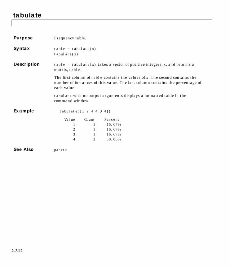
tabulate
2-312
2tabulatePurpose Frequency table.
Syntax table = tabulate(x)tabulate(x)
Description table = tabulate(x) takes a vector of positive integers, x, and returns amatrix, table.
The first column of table contains the values of x. The second contains thenumber of instances of this value. The last column contains the percentage ofeach value.
tabulate with no output arguments displays a formatted table in thecommand window.
Example tabulate([1 2 4 4 3 4])
Value Count Percent 1 1 16.67% 2 1 16.67% 3 1 16.67% 4 3 50.00%
See Also pareto
tblread
2-313
2tblreadPurpose Read tabular data from the file system.
Syntax [data,varnames,casenames] = tblread[data,varnames,casenames] = tblread('filename')[data,varnames,casenames] = tblread('filename','delimiter')
Description [data,varnames,casenames] = tblread displays the File Open dialog box forinteractive selection of the tabular data file. The file format has variable namesin the first row, case names in the first column and data starting in the (2,2)position.
[data,varnames,casenames] = tblread(filename) allows command linespecification of the name of a file in the current directory, or the completepathname of any file.
[data,varnames,casenames] = tblread(filename,'delimiter') allowsspecification of the field 'delimiter' in the file. Accepted values are 'tab','space', or 'comma'.
tblread returns the data read in three values.
Return Value Description
data Numeric matrix with a value for each variable-case pair.
varnames String matrix containing the variable names in the firstrow.
casenames String matrix containing the names of each case in thefirst column.
tblread
2-314
Example [data,varnames,casenames] = tblread('sat.dat')
data =
470 530 520 480
varnames =
Male Female
casenames =
Verbal Quantitative
See Also caseread, tblwrite, tdfread

tblwrite
2-315
2tblwritePurpose Writes tabular data to the file system.
Syntax tblwrite(data,'varnames','casenames')tblwrite(data,'varnames','casenames','filename')
Description tblwrite(data,'varnames','casenames') displays the File Open dialog boxfor interactive specification of the tabular data output file. The file format hasvariable names in the first row, case names in the first column and datastarting in the (2,2) position.
'varnames' is a string matrix containing the variable names. 'casenames' isa string matrix containing the names of each case in the first column. data isa numeric matrix with a value for each variable-case pair.
tblwrite(data,'varnames','casenames','filename') allows command linespecification of a file in the current directory, or the complete pathname of anyfile in the string 'filename'.
Example Continuing the example from tblread:
tblwrite(data,varnames,casenames,'sattest.dat')type sattest.dat
Male FemaleVerbal 470 530Quantitative 520 480
See Also casewrite, tblread

tcdf
2-316
2tcdfPurpose Student’s t cumulative distribution function (cdf).
Syntax P = tcdf(X,V)
Description P = tcdf(X,V) computes Student’s t cdf at each of the values in X using thecorresponding degrees of freedom in V. Vector or matrix inputs for X and V mustbe the same size. A scalar input is expanded to a constant matrix with the samedimensions as the other inputs. The parameters in V must be positive integers.
The t cdf is
The result, p, is the probability that a single observation from the t distributionwith ν degrees of freedom will fall in the interval (-∞ x].
Examples Suppose 10 samples of Guinness beer have a mean alcohol content of 5.5% byvolume and the standard deviation of these samples is 0.5%. What is theprobability that the true alcohol content of Guinness beer is less than 5%?
t = (5.0 - 5.5) / 0.5;probability = tcdf(t,10 - 1)
probability =
0.1717
See Also cdf, tinv, tpdf, trnd, tstat
p F x ν( )Γ ν 1+
2------------� �� �
Γ ν2---� �� �
----------------------1νπ
----------1
1 t2
ν-----+
� �� �
ν 1+2
------------------------------------------- td
∞–
x
�= =

tdfread
2-317
2tdfreadPurpose Read file containing tab-delimited numeric and text values.
Syntax tdfreadtdfread('filename')tdfread('filename','delimiter')
Description tdfread displays the File Open dialog box for interactive selection of the datafile. The file should consist of columns of values, separated by tabs, and withcolumn names in the first line of the file. Each column is read from the file andassigned to a variable with the specified name. If all values for a column arenumeric, the variable is converted to numbers; otherwise the variable is astring matrix. After all values are imported, tdfread displays informationabout the imported values using the format of the whos command.
tdfread('filename') allows command line specification of the name of a filein the current directory, or the complete pathname of any file.
tdfread('filename','delimiter') indicates that the character specified by'delimiter' separates columns in the file. Accepted values are:
• ' ' or 'space'
• '\t' or 'tab'
• ',' or 'comma'
• ';' or 'semi'
• '|' or 'bar'
The default delimiter is 'tab'.
Example type sat2.dat
Test,Gender,ScoreVerbal,Mail,470Verbal,Female,530Quantitative,Male,520Quantitative,Female,480tdfread('sat2.dat',',')

tdfread
2-318
Name Size Bytes Class
Gender 4x6 48 char array Score 4x1 32 double array Test 4x12 96 char array
Grand total is 76 elements using 176 bytes
See Also tblread

tinv
2-319
2tinvPurpose Inverse of the Student’s t cumulative distribution function (cdf).
Syntax X = tinv(P,V)
Description X = tinv(P,V) computes the inverse of Student’s t cdf with parameter V forthe corresponding probabilities in P. Vector or matrix inputs for P and V mustbe the same size. A scalar input is expanded to a constant matrix with the samedimensions as the other inputs. The degrees of freedom in V must be positiveintegers, and the values in P must lie on the interval [0 1].
The t inverse function in terms of the t cdf is
where
The result, x, is the solution of the cdf integral with parameter ν, where yousupply the desired probability p.
Examples What is the 99th percentile of the t distribution for one to six degrees offreedom?
percentile = tinv(0.99,1:6)
percentile =
31.8205 6.9646 4.5407 3.7469 3.3649 3.1427
See Also icdf, tcdf, tpdf, trnd, tstat
x F 1– p ν( ) x:F x ν( ) p={ }= =
p F x ν( )Γ ν 1+
2------------� �� �
Γ ν2---� �� �
----------------------1νπ
----------1
1 t2
ν-----+
� �� �
ν 1+2
------------------------------------------- td
∞–
x
�= =
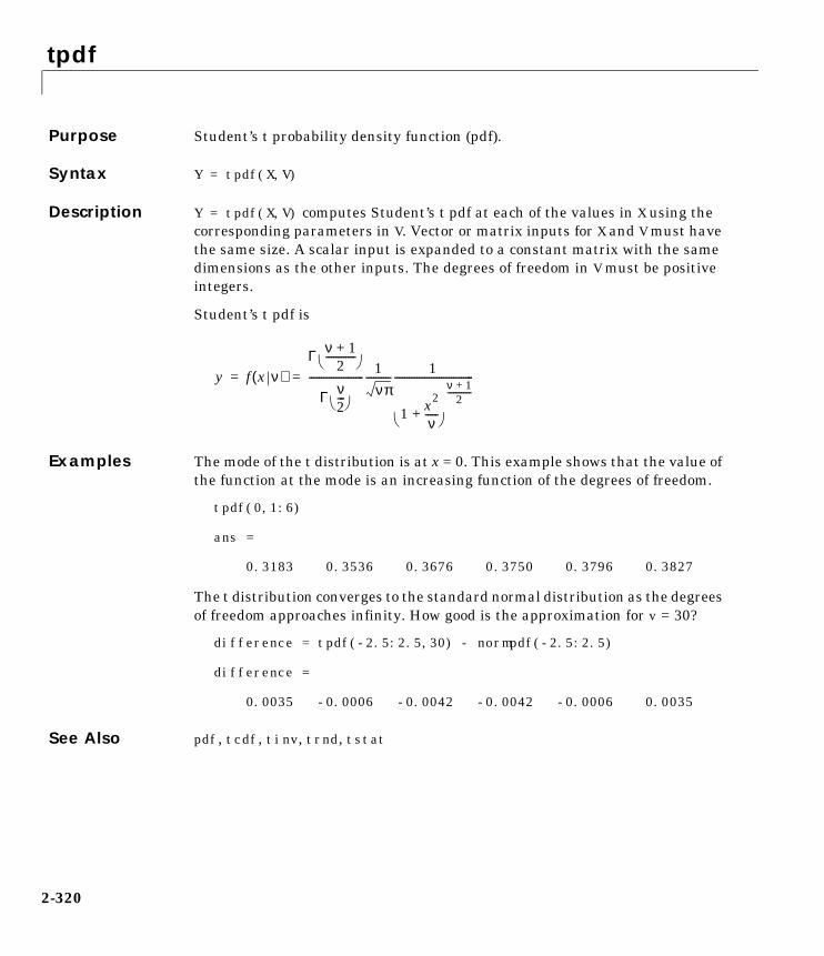
tpdf
2-320
2tpdfPurpose Student’s t probability density function (pdf).
Syntax Y = tpdf(X,V)
Description Y = tpdf(X,V) computes Student’s t pdf at each of the values in X using thecorresponding parameters in V. Vector or matrix inputs for X and V must havethe same size. A scalar input is expanded to a constant matrix with the samedimensions as the other inputs. The degrees of freedom in V must be positiveintegers.
Student’s t pdf is
Examples The mode of the t distribution is at x = 0. This example shows that the value ofthe function at the mode is an increasing function of the degrees of freedom.
tpdf(0,1:6)
ans =
0.3183 0.3536 0.3676 0.3750 0.3796 0.3827
The t distribution converges to the standard normal distribution as the degreesof freedom approaches infinity. How good is the approximation for v = 30?
difference = tpdf(-2.5:2.5,30) - normpdf(-2.5:2.5)
difference =
0.0035 -0.0006 -0.0042 -0.0042 -0.0006 0.0035
See Also pdf, tcdf, tinv, trnd, tstat
y f x ν( )Γ ν 1+
2------------� �� �
Γ ν2---� �� �
----------------------1νπ
----------1
1 x2
ν-----+
� �� �
ν 1+2
--------------------------------------------= =
trimmean
2-321
2trimmeanPurpose Mean of a sample of data excluding extreme values.
Syntax m = trimmean(X,percent)
Description m = trimmean(X,percent) calculates the mean of a sample X excluding thehighest and lowest percent/2 of the observations. The trimmed mean is arobust estimate of the location of a sample. If there are outliers in the data, thetrimmed mean is a more representative estimate of the center of the body of thedata. If the data is all from the same probability distribution, then the trimmedmean is less efficient than the sample average as an estimator of the locationof the data.
Examples This example shows a Monte Carlo simulation of the efficiency of the 10%trimmed mean relative to the sample average for normal data.
x = normrnd(0,1,100,100);m = mean(x);trim = trimmean(x,10);sm = std(m);strim = std(trim);efficiency = (sm/strim).^2
efficiency =
0.9702
See Also mean, median, geomean, harmmean
trnd
2-322
2trndPurpose Random numbers from Student’s t distribution.
Syntax R = trnd(V)R = trnd(V,m)R = trnd(V,m,n)
Description R = trnd(V) generates random numbers from Student’s t distribution with Vdegrees of freedom. The size of R is the size of V.
R = trnd(V,m) generates random numbers from Student’s t distribution withV degrees of freedom, where m is a 1-by-2 vector that contains the row andcolumn dimensions of R.
R = trnd(V,m,n) generates random numbers from Student’s t distributionwith V degrees of freedom, where scalars m and n are the row and columndimensions of R.
Examples noisy = trnd(ones(1,6))
noisy =
19.7250 0.3488 0.2843 0.4034 0.4816 -2.4190
numbers = trnd(1:6,[1 6])
numbers =
-1.9500 -0.9611 -0.9038 0.0754 0.9820 1.0115
numbers = trnd(3,2,6)
numbers =
-0.3177 -0.0812 -0.6627 0.1905 -1.5585 -0.0433 0.2536 0.5502 0.8646 0.8060 -0.5216 0.0891
See Also tcdf, tinv, tpdf, tstat

tstat
2-323
2tstatPurpose Mean and variance for the Student’s t distribution.
Syntax [M,V] = tstat(NU)
Description [M,V] = tstat(NU) returns the mean and variance for Student’s t distributionwith parameters specified by NU. M and V are the same size as NU.
The mean of the Student’s t distribution with parameter ν is zero for values of νgreater than 1. If ν is one, the mean does not exist. The variance for values of νgreater than 2 is .
Examples Find the mean and variance for 1 to 30 degrees of freedom.
[m,v] = tstat(reshape(1:30,6,5))
m = NaN 0 0 0 0 0 0 0 0 0 0 0 0 0 0 0 0 0 0 0 0 0 0 0 0 0 0 0 0 0
v = NaN 1.4000 1.1818 1.1176 1.0870 NaN 1.3333 1.1667 1.1111 1.0833 3.0000 1.2857 1.1538 1.1053 1.0800 2.0000 1.2500 1.1429 1.1000 1.0769 1.6667 1.2222 1.1333 1.0952 1.0741 1.5000 1.2000 1.1250 1.0909 1.0714
Note that the variance does not exist for one and two degrees of freedom.
See Also tcdf, tinv, tpdf, trnd
ν ν 2–( )⁄

ttest
2-324
2ttestPurpose Hypothesis testing for a single sample mean.
Syntax h = ttest(x,m)h = ttest(x,m,alpha)[h,sig,ci] = ttest(x,m,alpha,tail)
Description h = ttest(x,m) performs a t-test at significance level 0.05 to determinewhether a sample from a normal distribution (in x) could have mean m whenthe standard deviation is unknown.
h = ttest(x,m,alpha) gives control of the significance level, alpha. Forexample if alpha = 0.01, and the result, h, is 1 you can reject the nullhypothesis at the significance level 0.01. If h is 0, you cannot reject the nullhypothesis at the alpha level of significance.
[h,sig,ci] = ttest(x,m,alpha,tail) allows specification of one- ortwo-tailed tests. tail is a flag that specifies one of three alternativehypotheses:
• tail = 0 specifies the alternative (default)
• tail = 1 specifies the alternative
• tail = -1 specifies the alternative
Output sig is the p-value associated with the T-statistic
where is the sample standard deviation and is the number of observationsin the sample. sig is the probability that the observed value of T could be aslarge or larger by chance under the null hypothesis that the mean of x is equalto m.
ci is a 1-alpha confidence interval for the true mean.
Example This example generates 100 normal random numbers with theoretical meanzero and standard deviation one. The observed mean and standard deviationare different from their theoretical values, of course. We test the hypothesisthat there is no true difference.
x m≠x m>x m<
T x m–
s n⁄--------------=
s n

ttest
2-325
Normal random number generator test.
x = normrnd(0,1,1,100);[h,sig,ci] = ttest(x,0)
h = 0
sig = 0.4474
ci = -0.1165 0.2620
The result h = 0 means that we cannot reject the null hypothesis. Thesignificance level is 0.4474, which means that by chance we would haveobserved values of T more extreme than the one in this example in 45 of 100similar experiments. A 95% confidence interval on the mean is[-0.1165 0.2620], which includes the theoretical (and hypothesized) mean ofzero.
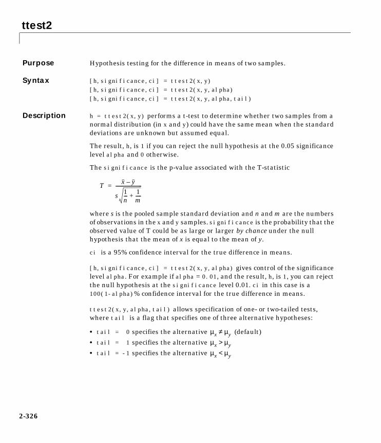
ttest2
2-326
2ttest2Purpose Hypothesis testing for the difference in means of two samples.
Syntax [h,significance,ci] = ttest2(x,y)[h,significance,ci] = ttest2(x,y,alpha)[h,significance,ci] = ttest2(x,y,alpha,tail)
Description h = ttest2(x,y) performs a t-test to determine whether two samples from anormal distribution (in x and y) could have the same mean when the standarddeviations are unknown but assumed equal.
The result, h, is 1 if you can reject the null hypothesis at the 0.05 significancelevel alpha and 0 otherwise.
The significance is the p-value associated with the T-statistic
where s is the pooled sample standard deviation and n and m are the numbersof observations in the x and y samples. significance is the probability that theobserved value of T could be as large or larger by chance under the nullhypothesis that the mean of x is equal to the mean of y.
ci is a 95% confidence interval for the true difference in means.
[h,significance,ci] = ttest2(x,y,alpha) gives control of the significancelevel alpha. For example if alpha = 0.01, and the result, h, is 1, you can rejectthe null hypothesis at the significance level 0.01. ci in this case is a100(1-alpha)% confidence interval for the true difference in means.
ttest2(x,y,alpha,tail) allows specification of one- or two-tailed tests,where tail is a flag that specifies one of three alternative hypotheses:
• tail = 0 specifies the alternative (default)
• tail = 1 specifies the alternative
• tail = -1 specifies the alternative
T x y–
s 1n---
1m-----+
-----------------------=
µx µy≠µx µy>µx µy<

ttest2
2-327
Examples This example generates 100 normal random numbers with theoretical mean 0and standard deviation 1. We then generate 100 more normal random numberswith theoretical mean 1/2 and standard deviation 1. The observed means andstandard deviations are different from their theoretical values, of course. Wetest the hypothesis that there is no true difference between the two means.Notice that the true difference is only one half of the standard deviation of theindividual observations, so we are trying to detect a signal that is only one halfthe size of the inherent noise in the process.
x = normrnd(0,1,100,1);y = normrnd(0.5,1,100,1);
[h,significance,ci] = ttest2(x,y)
h =1
significance =
0.0017
ci = -0.7352 -0.1720
The result h = 1 means that we can reject the null hypothesis. Thesignificance is 0.0017, which means that by chance we would have observedvalues of t more extreme than the one in this example in only 17 of 10,000similar experiments! A 95% confidence interval on the mean is[-0.7352 -0.1720], which includes the theoretical (and hypothesized) differenceof -0.5.

unidcdf
2-328
2unidcdfPurpose Discrete uniform cumulative distribution (cdf) function.
Syntax P = unidcdf(X,N)
Description P = unidcdf(X,N) computes the discrete uniform cdf at each of the values in Xusing the corresponding parameters in N. Vector or matrix inputs for X and Nmust have the same size. A scalar input is expanded to a constant matrix withthe same dimensions as the other inputs. The maximum observable values inN must be positive integers.
The discrete uniform cdf is
The result, p, is the probability that a single observation from the discreteuniform distribution with maximum N will be a positive integer less than orequal to x. The values x do not need to be integers.
Examples What is the probability of drawing a number 20 or less from a hat with thenumbers from 1 to 50 inside?
probability = unidcdf(20,50)
probability =
0.4000
See Also cdf, unidinv, unidpdf, unidrnd, unidstat
p F x N( ) floor x( )N
----------------------I 1 … N, ,( ) x( )= =

unidinv
2-329
2unidinvPurpose Inverse of the discrete uniform cumulative distribution function.
Syntax X = unidinv(P,N)
Description X = unidinv(P,N) returns the smallest positive integer X such that thediscrete uniform cdf evaluated at X is equal to or exceeds P. You can think of Pas the probability of drawing a number as large as X out of a hat with thenumbers 1 through N inside.
Vector or matrix inputs for N and P must have the same size, which is also thesize of X. A scalar input for N or P is expanded to a constant matrix with thesame dimensions as the other input. The values in P must lie on the interval[0 1] and the values in N must be positive integers.
Examples x = unidinv(0.7,20)
x =14
y = unidinv(0.7 + eps,20)
y =15
A small change in the first parameter produces a large jump in output. The cdfand its inverse are both step functions. The example shows what happens at astep.
See Also icdf, unidcdf, unidpdf, unidrnd, unidstat

unidpdf
2-330
2unidpdfPurpose Discrete uniform probability density function (pdf).
Syntax Y = unidpdf(X,N)
Description unidpdf(X,N) computes the discrete uniform pdf at each of the values in Xusing the corresponding parameters in N. Vector or matrix inputs for X and N must have the same size. A scalar input is expanded to a constant matrix withthe same dimensions as the other inputs. The parameters in N must be positiveintegers.
The discrete uniform pdf is
You can think of y as the probability of observing any one number between 1and n.
Examples For fixed n, the uniform discrete pdf is a constant.
y = unidpdf(1:6,10)
y = 0.1000 0.1000 0.1000 0.1000 0.1000 0.1000
Now fix x, and vary n.
likelihood = unidpdf(5,4:9)
likelihood =
0 0.2000 0.1667 0.1429 0.1250 0.1111
See Also pdf, unidcdf, unidinv, unidrnd, unidstat
y f x N( ) 1N----I 1 … N, ,( ) x( )= =

unidrnd
2-331
2unidrndPurpose Random numbers from the discrete uniform distribution.
Syntax R = unidrnd(N)R = unidrnd(N,mm)R = unidrnd(N,mm,nn)
Description The discrete uniform distribution arises from experiments equivalent todrawing a number from one to N out of a hat.
R = unidrnd(N) generates discrete uniform random numbers withmaximum N. The parameters in N must be positive integers. The size of R is thesize of N.
R = unidrnd(N,mm) generates discrete uniform random numbers withmaximum N, where mm is a 1-by-2 vector that contains the row and columndimensions of R.
R = unidrnd(N,mm,nn) generates discrete uniform random numbers withmaximum N, where scalars mm and nn are the row and column dimensions of R.
Examples In the Massachusetts lottery, a player chooses a four digit number. Generaterandom numbers for Monday through Saturday.
numbers = unidrnd(10000,1,6) - 1
numbers =
2189 470 6788 6792 9346
See Also unidcdf, unidinv, unidpdf, unidstat

unidstat
2-332
2unidstatPurpose Mean and variance for the discrete uniform distribution.
Syntax [M,V] = unidstat(N)
Description [M,V] = unidstat(N) returns the mean and variance for the discrete uniformdistribution with parameter N.
The mean of the discrete uniform distribution with parameter N is .The variance is .
Examples [m,v] = unidstat(1:6)
m = 1.0000 1.5000 2.0000 2.5000 3.0000 3.5000
v = 0 0.2500 0.6667 1.2500 2.0000 2.9167
See Also unidcdf, unidinv, unidpdf, unidrnd
N 1+( ) 2⁄N2 1–( ) 12⁄

unifcdf
2-333
2unifcdfPurpose Continuous uniform cumulative distribution function (cdf).
Syntax P = unifcdf(X,A,B)
Description P = unifcdf(X,A,B) computes the uniform cdf at each of the values in X usingthe corresponding parameters in A and B (the minimum and maximum values,respectively). Vector or matrix inputs for X, A, and B must all have the samesize. A scalar input is expanded to a constant matrix with the same dimensionsas the other inputs.
The uniform cdf is
The standard uniform distribution has A = 0 and B = 1.
Examples What is the probability that an observation from a standard uniformdistribution will be less than 0.75?
probability = unifcdf(0.75)
probability =
0.7500
What is the probability that an observation from a uniform distribution witha = -1 and b = 1 will be less than 0.75?
probability = unifcdf(0.75,-1,1)
probability =
0.8750
See Also cdf, unifinv, unifit, unifpdf, unifrnd, unifstat
p F x a b,( ) x a–b a–------------I a b,[ ] x( )= =

unifinv
2-334
2unifinvPurpose Inverse continuous uniform cumulative distribution function (cdf).
Syntax X = unifinv(P,A,B)
Description X = unifinv(P,A,B) computes the inverse of the uniform cdf with parametersA and B (the minimum and maximum values, respectively) at the correspondingprobabilities in P. Vector or matrix inputs for P, A, and Bmust all have the samesize. A scalar input is expanded to a constant matrix with the same dimensionsas the other inputs.
The inverse of the uniform cdf is
The standard uniform distribution has A = 0 and B = 1.
Examples What is the median of the standard uniform distribution?
median_value = unifinv(0.5)
median_value =
0.5000
What is the 99th percentile of the uniform distribution between -1 and 1?
percentile = unifinv(0.99,-1,1)
percentile =
0.9800
See Also icdf, unifcdf, unifit, unifpdf, unifrnd, unifstat
x F 1– p a b,( ) a p a b–( )I 0 1,[ ] p( )+= =

unifit
2-335
2unifitPurpose Parameter estimates for uniformly distributed data.
Syntax [ahat,bhat] = unifit(X)[ahat,bhat,ACI,BCI] = unifit(X)[ahat,bhat,ACI,BCI] = unifit(X,alpha)
Description [ahat,bhat] = unifit(X) returns the maximum likelihood estimates (MLEs)of the parameters of the uniform distribution given the data in X.
[ahat,bhat,ACI,BCI] = unifit(X) also returns 95% confidence intervals,ACI and BCI, which are matrices with two rows. The first row contains thelower bound of the interval for each column of the matrix X. The second rowcontains the upper bound of the interval.
[ahat,bhat,ACI,BCI] = unifit(X,alpha) allows control of the confidencelevel alpha. For example, if alpha = 0.01 then ACI and BCI are 99% confidenceintervals.
Example r = unifrnd(10,12,100,2);[ahat,bhat,aci,bci] = unifit(r)
ahat =
10.0154 10.0060
bhat =
11.9989 11.9743
aci =
9.9551 9.9461 10.0154 10.0060
bci =
11.9989 11.9743 12.0592 12.0341
See Also betafit, binofit, expfit, gamfit, normfit, poissfit, unifcdf, unifinv,unifpdf, unifrnd, unifstat, weibfit

unifpdf
2-336
2unifpdfPurpose Continuous uniform probability density function (pdf).
Syntax Y = unifpdf(X,A,B)
Description Y = unifpdf(X,A,B) computes the continuous uniform pdf at each of thevalues in X using the corresponding parameters in A and B. Vector or matrixinputs for X, A, and B must all have the same size. A scalar input is expandedto a constant matrix with the same dimensions as the other inputs. Theparameters in B must be greater than those in A.
The continuous uniform distribution pdf is
The standard uniform distribution has A = 0 and B = 1.
Examples For fixed a and b, the uniform pdf is constant.
x = 0.1:0.1:0.6;y = unifpdf(x)
y = 1 1 1 1 1 1
What if x is not between a and b?
y = unifpdf(-1,0,1)
y = 0
See Also pdf, unifcdf, unifinv, unifrnd, unifstat
y f x a b,( ) 1b a–------------I a b,[ ] x( )= =

unifrnd
2-337
2unifrndPurpose Random numbers from the continuous uniform distribution.
Syntax R = unifrnd(A,B)R = unifrnd(A,B,m)R = unifrnd(A,B,m,n)
Description R = unifrnd(A,B) generates uniform random numbers with parameters Aand B. Vector or matrix inputs for A and B must have the same size, which isalso the size of R. A scalar input for A or B is expanded to a constant matrix withthe same dimensions as the other input.
R = unifrnd(A,B,m) generates uniform random numbers with parameters Aand B, where m is a 1-by-2 vector that contains the row and column dimensionsof R.
R = unifrnd(A,B,m,n) generates uniform random numbers with parametersA and B, where scalars m and n are the row and column dimensions of R.
Examples random = unifrnd(0,1:6)
random =
0.2190 0.0941 2.0366 2.7172 4.6735 2.3010
random = unifrnd(0,1:6,[1 6])
random =
0.5194 1.6619 0.1037 0.2138 2.6485 4.0269
random = unifrnd(0,1,2,3)
random =
0.0077 0.0668 0.6868 0.3834 0.4175 0.5890
See Also unifcdf, unifinv, unifpdf, unifstat
unifstat
2-338
2unifstatPurpose Mean and variance for the continuous uniform distribution.
Syntax [M,V] = unifstat(A,B)
Description [M,V] = unifstat(A,B) returns the mean and variance for the continuousuniform distribution with parameters specified by A and B. Vector or matrixinputs for A and B must have the same size, which is also the size of M and V. Ascalar input for A or B is expanded to a constant matrix with the samedimensions as the other input.
The mean of the continuous uniform distribution with parameters a and b is, and the variance is .
Examples a = 1:6;b = 2.∗a;[m,v] = unifstat(a,b)
m = 1.5000 3.0000 4.5000 6.0000 7.5000 9.0000
v = 0.0833 0.3333 0.7500 1.3333 2.0833 3.0000
See Also unifcdf, unifinv, unifpdf, unifrnd
a b+( ) 2⁄ b a–( )2 12⁄
var
2-339
2varPurpose Variance of a sample.
Syntax y = var(X)y = var(X,1)y = var(X,w)
Description y = var(X) computes the variance of the data in X. For vectors, var(x) is thevariance of the elements in x. For matrices, var(X) is a row vector containingthe variance of each column of X.
y = var(x) normalizes by n-1 where n is the sequence length. For normallydistributed data, this makes var(x) the minimum variance unbiased estimatorMVUE of σ 2(the second parameter).
y = var(x,1) normalizes by n and yields the second moment of the sampledata about its mean (moment of inertia).
y = var(X,w) computes the variance using the vector of positive weights w.The number of elements in w must equal the number of rows in the matrix X.For vector x, w and x must match in length.
var supports both common definitions of variance. Let SS be the sum ofthe squared deviations of the elements of a vector x from their mean. Then,var(x) = SS/(n-1) is the MVUE, and var(x,1) = SS/n is the maximumlikelihood estimator (MLE) of σ 2.
var
2-340
Examples x = [-1 1];w = [1 3];v1 = var(x)
v1 = 2
v2 = var(x,1)
v2 = 1
v3 = var(x,w)
v3 = 0.7500
See Also cov, std

weibcdf
2-341
2weibcdfPurpose Weibull cumulative distribution function (cdf).
Syntax P = weibcdf(X,A,B)
Description P = weibcdf(X,A,B) computes the Weibull cdf at each of the values in X usingthe corresponding parameters in A and B. Vector or matrix inputs for X, A, andB must all have the same size. A scalar input is expanded to a constant matrixwith the same dimensions as the other inputs. The parameters in A and B mustbe positive.
The Weibull cdf is
Examples What is the probability that a value from a Weibull distribution withparameters a = 0.15 and b = 0.24 is less than 500?
probability = weibcdf(500,0.15,0.24)
probability =
0.4865
How sensitive is this result to small changes in the parameters?
[A,B] = meshgrid(0.1:0.05:0.2,0.2:0.05:0.3);probability = weibcdf(500,A,B)
probability =
0.2929 0.4054 0.5000 0.3768 0.5080 0.6116 0.4754 0.6201 0.7248
See Also cdf, weibfit, weibinv, weiblike, weibpdf, weibplot, weibrnd, weibstat
p F x a b,( ) abtb 1– e atb– td0
x
� 1 e axb– I 0 ∞,( ) x( )–= = =

weibfit
2-342
2weibfitPurpose Parameter estimates and confidence intervals for Weibull data.
Syntax phat = weibfit(x)[phat,pci] = weibfit(x)[phat,pci] = weibfit(x,alpha)
Description phat = weibfit(x) returns the maximum likelihood estimates, phat, of theparameters of the Weibull distribution given the values in vector x, which mustbe positive. phat is a two-element row vector: phat(1) estimates the Weibullparameter a, and phat(2) estimates the Weibull parameter b in the pdf
[phat,pci] = weibfit(x) also returns 95% confidence intervals in thetwo-row matrix pci. The first row contains the lower bound of the confidenceinterval, and the second row contains the upper bound. The columns of pcicorrespond to the columns of phat.
[phat,pci] = weibfit(x,alpha) allows control over the confidence intervalreturned, 100(1-alpha)%.
Example r = weibrnd(0.5,0.8,100,1);[phat,pci] = weibfit(r)
phat =
0.4746 0.7832
pci =
0.3851 0.6367 0.5641 0.9298
See Also betafit, binofit, expfit, gamfit, normfit, poissfit, unifit, weibcdf,weibinv, weiblike, weibpdf, weibplot, weibrnd, weibstat
y f x a b,( ) abxb 1– e axb– I 0 ∞,( ) x( )= =

weibinv
2-343
2weibinvPurpose Inverse of the Weibull cumulative distribution function.
Syntax X = weibinv(P,A,B)
Description X = weibinv(P,A,B) computes the inverse of the Weibull cdf with parametersA and B for the corresponding probabilities in P. Vector or matrix inputs for P,A, and B must all have the same size. A scalar input is expanded to a constantmatrix with the same dimensions as the other inputs. The parameters in A andB must be positive.
The inverse of the Weibull cdf is
Examples A batch of light bulbs have lifetimes (in hours) distributed Weibull withparameters a = 0.15 and b = 0.24. What is the median lifetime of the bulbs?
life = weibinv(0.5,0.15,0.24)
life =
588.4721
What is the 90th percentile?
life = weibinv(0.9,0.15,0.24)
life =
8.7536e+04
See Also icdf, weibcdf, weibfit, weiblike, weibpdf, weibplot, weibrnd, weibstat
x F 1– p a b,( ) 1a---
11 p–------------� �� �ln
1b---
I 0 1,[ ] p( )= =

weiblike
2-344
2weiblikePurpose Weibull negative log-likelihood function.
Syntax logL = weiblike(params,data)[logL,avar] = weiblike(params,data)
Description logL = weiblike(params,data) returns the Weibull log-likelihood withparameters params(1) = a and params(2) = b given the data xi.
[logL,avar] = weiblike(params,data) also returns avar, which is theasymptotic variance-covariance matrix of the parameter estimates if thevalues in params are the maximum likelihood estimates. avar is the inverse ofFisher's information matrix. The diagonal elements of avar are the asymptoticvariances of their respective parameters.
The Weibull negative log-likelihood is
weiblike is a utility function for maximum likelihood estimation.
Example This example continues the example from weibfit.
r = weibrnd(0.5,0.8,100,1);[logL,info] = weiblike([0.4746 0.7832],r)
logL =
203.8216
info =
0.0021 0.0022 0.0022 0.0056
Reference Patel, J. K., C. H. Kapadia, and D. B. Owen, Handbook of StatisticalDistributions, Marcel-Dekker, 1976.
See Also betalike, gamlike, mle, weibcdf, weibfit, weibinv, weibpdf, weibplot,weibrnd, weibstat
Llog– f a b, xi( )i 1=∏log– f a b, xi( )log
i 1=
n
�–= =

weibpdf
2-345
2weibpdfPurpose Weibull probability density function (pdf).
Syntax Y = weibpdf(X,A,B)
Description Y = weibpdf(X,A,B) computes the Weibull pdf at each of the values in X usingthe corresponding parameters in A and B. Vector or matrix inputs for X, A, andB must all have the same size. A scalar input is expanded to a constant matrixwith the same dimensions as the other input. The parameters in A and B mustall be positive.
The Weibull pdf is
Some references refer to the Weibull distribution with a single parameter. Thiscorresponds to weibpdf with A = 1.
Examples The exponential distribution is a special case of the Weibull distribution.
lambda = 1:6;y = weibpdf(0.1:0.1:0.6,lambda,1)
y =
0.9048 1.3406 1.2197 0.8076 0.4104 0.1639
y1 = exppdf(0.1:0.1:0.6,1./lambda)
y1 =
0.9048 1.3406 1.2197 0.8076 0.4104 0.1639
Reference Devroye, L., Non-Uniform Random Variate Generation. Springer-Verlag. NewYork, 1986.
See Also pdf, weibcdf, weibfit, weibinv, weiblike, weibplot, weibrnd, weibstat
y f x a b,( ) abxb 1– e axb– I 0 ∞,( ) x( )= =
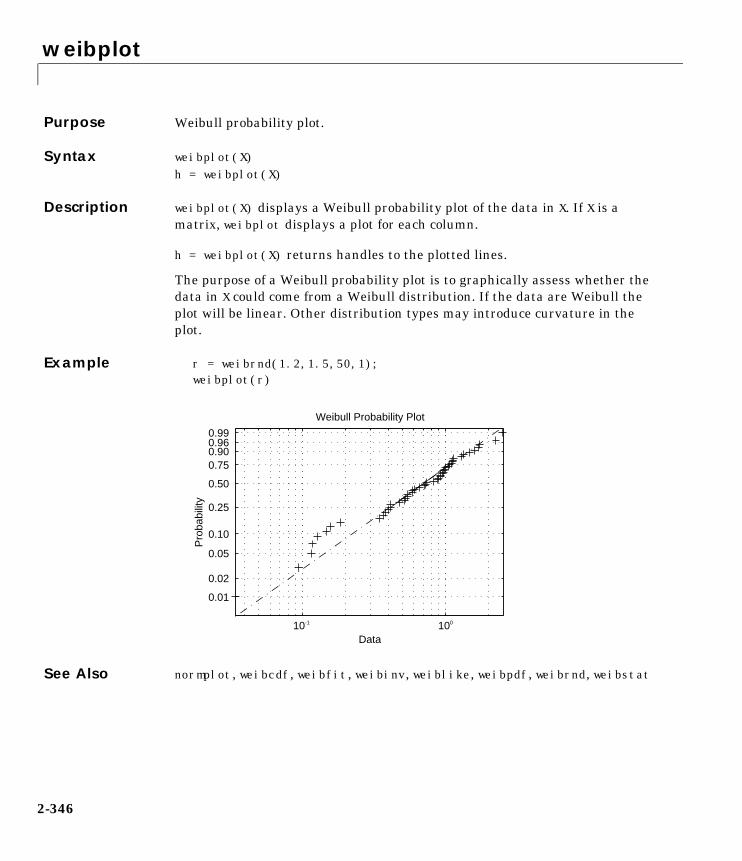
weibplot
2-346
2weibplotPurpose Weibull probability plot.
Syntax weibplot(X)h = weibplot(X)
Description weibplot(X) displays a Weibull probability plot of the data in X. If X is amatrix, weibplot displays a plot for each column.
h = weibplot(X) returns handles to the plotted lines.
The purpose of a Weibull probability plot is to graphically assess whether thedata in X could come from a Weibull distribution. If the data are Weibull theplot will be linear. Other distribution types may introduce curvature in theplot.
Example r = weibrnd(1.2,1.5,50,1);weibplot(r)
See Also normplot, weibcdf, weibfit, weibinv, weiblike, weibpdf, weibrnd, weibstat
10-1 100
0.01
0.02
0.05
0.10
0.25
0.50
0.75 0.90 0.96 0.99
Data
Pro
babi
lity
Weibull Probability Plot

weibrnd
2-347
2weibrndPurpose Random numbers from the Weibull distribution.
Syntax R = weibrnd(A,B)R = weibrnd(A,B,m)R = weibrnd(A,B,m,n)
Description R = weibrnd(A,B) generates Weibull random numbers with parameters Aand B. Vector or matrix inputs for A and B must have the same size, which isalso the size of R. A scalar input for A or B is expanded to a constant matrix withthe same dimensions as the other input.
R = weibrnd(A,B,m) generates Weibull random numbers with parameters Aand B, where m is a 1-by-2 vector that contains the row and column dimensionsof R.
R = weibrnd(A,B,m,n) generates Weibull random numbers with parametersA and B, where scalars m and n are the row and column dimensions of R.
Devroye refers to the Weibull distribution with a single parameter; this isweibrnd with A = 1.
Examples n1 = weibrnd(0.5:0.5:2,0.5:0.5:2)
n1 = 0.0093 1.5189 0.8308 0.7541
n2 = weibrnd(1/2,1/2,[1 6])
n2 = 29.7822 0.9359 2.1477 12.6402 0.0050 0.0121
Reference Devroye, L., Non-Uniform Random Variate Generation. Springer-Verlag. NewYork, 1986.
See Also weibcdf, weibfit, weibinv, weiblike, weibpdf, weibplot, weibstat

weibstat
2-348
2weibstatPurpose Mean and variance for the Weibull distribution.
Syntax [M,V] = weibstat(A,B)
Description [M,V] = weibstat(A,B) returns the mean and variance for the Weibulldistribution with parameters specified by A and B. Vector or matrix inputs forA and Bmust have the same size, which is also the size of M and V. A scalar inputfor A or B is expanded to a constant matrix with the same dimensions as theother input.
The mean of the Weibull distribution with parameters a and b is
and the variance is
Examples [m,v] = weibstat(1:4,1:4)
m = 1.0000 0.6267 0.6192 0.6409
v = 1.0000 0.1073 0.0506 0.0323
weibstat(0.5,0.7)
ans =
3.4073
See Also weibcdf, weibfit, weibinv, weiblike, weibpdf, weibplot, weibrnd
a
1b---–
Γ 1 b 1–+( )
a
2b---–
Γ 1 2b 1–+( ) Γ2 1 b 1–
+( )–

x2fx
2-349
2x2fxPurpose Transform a factor settings matrix to a design matrix.
Syntax D = x2fx(X)D = x2fx(X,'model')
Description D = x2fx(X) transforms a matrix of system inputs, X, to a design matrix for alinear additive model with a constant term.
D = x2fx(X,'model') allows control of the order of the regressionmodel.'model' can be one of these strings:
• 'interaction' – includes constant, linear, and cross product terms
• 'quadratic' – includes interactions and squared terms
• 'purequadratic' – includes constant, linear, and squared terms
Alternatively model can be a matrix of terms. In this case, each row of modelrepresents one term. The value in a column is the exponent to which the samecolumn in X for that term should be raised. This allows for models withpolynomial terms of arbitrary order.
x2fx is a utility function for rstool, regstats, and cordexch.
Example x = [1 2 3;4 5 6]'; model = 'quadratic';D = x2fx(x,model)
D =
1 1 4 4 1 16 1 2 5 10 4 25 1 3 6 18 9 36
Let x1 be the first column of x and x2 be the second. Then the first column of Dis the constant term, the second column is x1, the third column is x2, the fourthcolumn is x1x2, the fifth column is x1
2, and the last columns is x22.
See Also rstool, cordexch, rowexch, regstats

xbarplot
2-350
2xbarplotPurpose X-bar chart for Statistical Process Control.
Syntax xbarplot(DATA)xbarplot(DATA,conf)xbarplot(DATA,conf,specs,'sigmaest')[outlier,h] = xbarplot(...)
Description xbarplot(DATA) displays an x-bar chart of the grouped responses in DATA. Therows of DATA contain replicate observations taken at a given time, and must bein time order. The graph contains the sample mean for each group, a centerline at the average value, and upper and lower control limits. The limits areplaced at a three-sigma distance on either side of the center line, where sigmais an estimate of the standard deviation of . If the process is in control, fewerthan 3 out of 1000 observations would be expected to fall outside the controllimits by random chance. So if you observe points outside the limits, you cantake this as evidence that the process is not in control.
xbarplot(DATA,conf) allows control of the confidence level of the upper andlower plotted confidence limits. The default conf = 0.9973 producesthree-sigma limits.
norminv(1 - (1-.9973)/2)
ans = 3
To get k-sigma limits, use the expression 1-2*(1-normcdf(k)). For example,the correct conf value for 2-sigma limits is 0.9545, as shown below.
k = 2;1-2*(1-normcdf(k))
ans = 0.9545
xbarplot(DATA,conf,specs) plots the specification limits in the two elementvector specs.
xx
x

xbarplot
2-351
xbarplot(DATA,conf,specs,'sigmaest') specifies how xbarplot shouldestimate the standard deviation. Acceptable values are:
• 's' – use the average of the group standard deviations (default)
• 'v' – use the square root of a pooled variance estimate
• 'r' – use the average range with each group; requires 25 or fewerobservations per group
[outlier,h] = xbarplot(DATA,conf,specs) returns outlier, a vector ofindices to the rows where the mean of DATA is out of control, and h, a vector ofhandles to the plotted lines.
Example Plot an x-bar chart of measurements on newly machined parts, taken at onehour intervals for 36 hours. Each row of the runout matrix contains themeasurements for four parts chosen at random. The values indicate, inthousandths of an inch, the amount the part radius differs from the targetradius.
load partsxbarplot(runout,0.999,[-0.5 0.5])
The points in groups 21 and 25 are out of control, so the mean in those groupswas higher than would be expected by random chance alone. There is evidencethat the process was not in control when those measurements were collected.
0 5 10 15 20 25 30 35 40−0.5
−0.4
−0.3
−0.2
−0.1
0
0.1
0.2
0.3
0.4
0.5
21 25
UCL
LCL
CL
Xbar ChartUSL
LSL
Samples
Mea
sure
men
ts

xbarplot
2-352
See Also capaplot, histfit, ewmaplot, schart

zscore
2-353
2zscorePurpose Standardized Z score.
Syntax Z = zscore(D)
Description Z = zscore(D) returns the deviation of each column of D from its mean,normalized by its standard deviation. This is known as the Z score of D.
For column vector V, the Z score is Z = (V-mean(V))./std(V).
ztest
2-354
2ztestPurpose Hypothesis testing for the mean of one sample with known variance.
Syntax h = ztest(x,m,sigma)h = ztest(x,m,sigma,alpha)[h,sig,ci,zval] = ztest(x,m,sigma,alpha,tail)
Description h = ztest(x,m,sigma) performs a Z test at significance level 0.05 todetermine whether a sample x from a normal distribution with standarddeviation sigma could have mean m.
h = ztest(x,m,sigma,alpha) gives control of the significance level alpha. Forexample, if alpha = 0.01 and the result is h = 1, you can reject the nullhypothesis at the significance level 0.01. If h = 0, you cannot reject the nullhypothesis at the alpha level of significance.
[h,sig,ci] = ztest(x,m,sigma,alpha,tail) allows specification of one- ortwo-tailed tests, where tail is a flag that specifies one of three alternativehypotheses:
• tail = 0 specifies the alternative (default)
• tail = 1 specifies the alternative
• tail = -1 specifies the alternative
zval is the value of the Z statistic
where is the number of observations in the sample.
sig is the probability that the observed value of Z could be as large or larger bychance under the null hypothesis that the mean of x is equal to m.
ci is a 1-alpha confidence interval for the true mean.
x m≠x m>x m<
z x m–
σ n⁄---------------=
n

ztest
2-355
Example This example generates 100 normal random numbers with theoretical meanzero and standard deviation one. The observed mean and standard deviationare different from their theoretical values, of course. We test the hypothesisthat there is no true difference.
x = normrnd(0,1,100,1);m = mean(x)m = 0.0727
[h,sig,ci] = ztest(x,0,1)
h = 0
sig = 0.4669
ci = -0.1232 0.2687
The result, h = 0, means that we cannot reject the null hypothesis. Thesignificance level is 0.4669, which means that by chance we would haveobserved values of Z more extreme than the one in this example in 47 of 100similar experiments. A 95% confidence interval on the mean is[-0.1232 0.2687], which includes the theoretical (and hypothesized) mean ofzero.

ztest
2-356

I-1
Index
Aabsolute deviation 1-45additive effects 1-73alternative hypothesis 1-105analysis of variance 1-23ANOVA 1-68anova1 2-12, 2-17, 2-160, 2-190anova2 2-12, 2-23, 2-27, 2-102, 2-106aoctool 1-153average linkage 2-179
Bbacteria counts 1-69barttest 2-14baseball odds 2-45, 2-47Bernoulli random variables 2-49beta distribution 1-12, 1-13betacdf 2-4, 2-37betafit 2-4, 2-38betainv 2-6, 2-40betalike 2-4, 2-41betapdf 2-5, 2-42betarnd 2-7, 2-43betastat 2-9, 2-44binocdf 2-4, 2-45binofit 2-4, 2-46binoinv 2-6, 2-47binomial distribution 1-12, 1-15binopdf 2-5, 2-48binornd 2-7, 2-49binostat 2-9, 2-50bootstrap 2-51bootstrap sampling 1-50box plots 1-128boxplot 2-11, 2-54
Ccapability studies 1-141capable 2-11, 2-56capaplot 2-11caseread 2-14, 2-60casewrite 2-14, 2-61cdf 1-6, 1-7cdf 2-4, 2-62census 2-15Central Limit Theorem 1-32centroid linkage 2-179Chatterjee and Hadi example 1-85chi2cdf 2-4, 2-65chi2inv 2-6, 2-66chi2pdf 2-5, 2-67chi2rnd 2-8, 2-68chi2stat 2-9, 2-69chi-square distribution 1-12, 1-17circuit boards 2-48cities 2-15City Block metric
in cluster analysis 2-256classify 2-70cluster 2-12, 2-71cluster analysis 1-53
computing inconsistency coefficient 1-60,2-155
creating clusters from data 2-73creating clusters from linkage output 1-64,
2-71creating the cluster tree 1-56, 2-178determining proximity 1-54, 2-255evaluating cluster formation 1-59, 2-76formatting distance information 1-56, 2-308overview 1-53plotting the cluster tree 1-58, 2-85

Index
I-2
clusterdata 2-12, 2-73coin 2-122combnk 2-75complete linkage 2-179confidence intervals
hypothesis tests 1-106nonlinear regression 1-103
control charts 1-138EWMA charts 1-140S charts 1-139Xbar charts 1-138
conventions in our documentation (table) xviiicophenet 2-12, 2-76
using 1-59cophenetic correlation coefficient 2-76
defined 1-59cordexch 2-13, 2-78corrcoef 2-79cov 2-80Cp index 1-142, 2-56Cpk index 1-142, 2-56crosstab 2-81cumulative distribution function (cdf) 1-6
Ddata 2-3daugment 2-13, 2-83dcovary 2-13, 2-84demos 1-153, 2-3
design of experiments 1-170polynomial curve fitting 1-156probability distributions 1-154random number generation 1-169
dendrogram 2-12, 2-85, 2-194using 1-58
depthin cluster analysis 1-61
descriptive statistics 1-43, 2-3Design of Experiments 1-143
D-optimal designs 1-147fractional factorial designs 1-145full factorial designs 1-144
discrete uniform distribution 1-12, 1-20discrim 2-15dissimilarity matrix
creating 1-54distributions 1-2, 1-5disttool 1-153, 2-15, 2-87DOE. See Design of ExperimentsD-optimal designs 1-147dummyvar 2-88
Eerf 1-32error function 1-32errorbar 2-11, 2-89estimate 1-157Euclidean distance
in cluster analysis 2-256EWMA charts 1-140ewmaplot 2-11, 2-90expcdf 2-4, 2-92expfit 2-4, 2-93expinv 2-7, 2-94exponential distribution 1-12, 1-21exppdf 2-5, 2-95exprnd 2-8, 2-96expstat 2-9, 2-97extrapolated 2-272

Index
I-3
FF distribution 1-12, 1-23F statistic 1-85fcdf 2-5, 2-98ff2n 2-13, 2-99file I/O 2-3finv 2-7, 2-100floppy disks 2-149fpdf 2-6, 2-101fractional factorial designs 1-145frnd 2-8, 2-110fstat 2-9, 2-111fsurfht 2-11, 2-112full factorial designs 1-144fullfact 2-13, 2-114furthest neighbor linkage 2-179
Ggamcdf 2-5, 2-115gamfit 2-4, 2-116gaminv 2-7, 2-117gamlike 2-4, 2-118gamma distribution 1-12, 1-25gampdf 2-6, 2-119gamrnd 2-8, 2-120gamstat 2-9, 2-121gas 2-15Gaussian 2-146geocdf 2-5, 2-122geoinv 2-7, 2-123geomean 2-10, 2-124geometric distribution 1-12, 1-27geopdf 2-6, 2-125geornd 2-8, 2-126geostat 2-9, 2-127gline 2-11, 2-128
gname 2-11, 2-135, 2-137grouped scatter plot 1-122grpstats 2-139, 2-142, 2-143Guinness beer 1-37, 2-316
Hhadamard 2-14hald 2-15harmmean 2-10, 2-145hat matrix 1-83hist 2-146histfit 2-11, 2-147histogram 1-169hogg 2-15Hotelling’s T squared 1-121hougen 2-148Hougen-Watson model 1-100hygecdf 2-5, 2-149hygeinv 2-7, 2-150hygepdf 2-6, 2-151hygernd 2-8, 2-152hygestat 2-9, 2-153hypergeometric distribution 1-12, 1-28hypotheses 1-23, 2-3hypothesis tests 1-105
Iicdf 2-154incomplete beta function 1-13incomplete gamma function 1-25inconsistency coefficient 1-61inconsistent 2-12, 2-155
using 1-61inspector 2-259interaction 1-74

Index
I-4
interpolated 2-311interquartile range (iqr) 1-45inverse cdf 1-6, 1-8iqr 2-10, 2-157
Kkurtosis 2-10, 2-172
Llawdata 2-15least squares 2-267leverage 2-174light bulbs, life of 2-94likelihood function 2-42linear 2-3linear models 1-68linkage 2-12, 2-175, 2-178
using 1-56logncdf 2-5, 2-181logninv 2-7, 2-182lognormal distribution 1-12, 1-30lognpdf 2-6, 2-184lognrnd 2-8, 2-185lognstat 2-9, 2-186lottery 2-331lsline 2-11, 2-187LU factorizations 2-266
Mmad 2-10, 2-188mahal 2-189Mahalanobis distance 2-189
in cluster analysis 2-256mean 1-6, 1-11
mean 2-10, 2-196Mean Squares (MS) 2-17measures of central tendency 1-43measures of dispersion 1-45median 2-10, 2-197mileage 2-15Minkowski metric
in cluster analysis 2-256mle 2-4, 2-198models
linear 1-68nonlinear 1-100
moment 2-10, 2-199Monte Carlo simulation 2-157moore 2-15multiple linear regression 1-82multivariate statistics 1-112mvnrnd 2-130, 2-200, 2-207, 2-293
Nnanmax 2-10, 2-209nanmean 2-10, 2-210nanmedian 2-10, 2-211nanmin 2-10, 2-212NaNs 1-46nanstd 2-10, 2-213nansum 2-10, 2-214nbincdf 2-5, 2-215nbininv 2-7, 2-216nbinpdf 2-6, 2-217nbinrnd 2-8, 2-218nbinstat 2-9, 2-219ncfcdf 2-5, 2-220ncfinv 2-7, 2-222ncfpdf 2-6, 2-223ncfrnd 2-8, 2-224

Index
I-5
ncfstat 2-9, 2-225nctcdf 2-5, 2-226nctinv 2-7, 2-227nctpdf 2-6, 2-228nctrnd 2-8, 2-229nctstat 2-9, 2-230ncx2cdf 2-5, 2-231ncx2inv 2-7, 2-233ncx2pdf 2-6, 2-234ncx2rnd 2-8, 2-235ncx2stat 2-9, 2-236nearest neighbor linkage 2-179negative binomial distribution 1-12, 1-31Newton’s method 2-117nlinfit 2-13, 2-237nlintool 1-153, 2-13, 2-238nlparci 2-13, 2-239nlpredci 2-13, 2-240noncentral chi-square distribution 1-12noncentral F distribution 1-12, 1-24noncentral t distribution 1-12, 1-38nonlinear 2-3nonlinear regression models 1-100normal distribution 1-12, 1-32normal probability plots 1-128, 1-129normalizing a dataset 1-55
using zscore 2-353normcdf 2-5, 2-242normdemo 2-11, 2-249normfit 2-4, 2-243norminv 2-7, 2-244normlike 2-4normpdf 2-6, 2-245normplot 2-11, 2-246normrnd 2-8, 2-248normstat 2-9, 2-250notches 2-54
null 1-105null hypothesis 1-105
Oone-way analysis of variance (ANOVA) 1-68outliers 1-44
Ppareto 2-11, 2-251parts 2-15Pascal, Blaise 1-15PCA. See Principal Components Analysispcacov 2-14, 2-252pcares 2-14, 2-253pdf 1-6pdf 2-254pdist 2-12, 2-255
using 1-54percentiles 1-49perms 2-258plots 1-49, 2-3poisscdf 2-5, 2-259poissfit 2-4, 2-261poissinv 2-7, 2-262Poisson distribution 1-12, 1-34poisspdf 2-6, 2-263poissrnd 2-8, 2-264poisstat 2-9, 2-265polyconf 2-13, 2-266polydata 2-16polyfit 2-13, 2-267polynomial 1-156polytool 1-153, 2-15, 2-33, 2-268polyval 2-13, 2-269popcorn 2-25, 2-108

Index
I-6
popcorn 2-15prctile 2-10, 2-270Principal Components Analysis 1-112
component scores 1-117component variances 1-120Hotelling’s T squared 1-121Scree plot 1-120
princomp 2-14, 2-271probability 2-3probability density function (pdf) 1-6probability distributions 1-5p-value 1-75, 1-106
Qqqplot 2-11, 2-272QR decomposition 1-83quality assurance 2-48quantile-quantile plots 1-128, 1-131
Rrandom 2-274random number generator 1-6random numbers 1-9randtool 1-153, 2-15, 2-87, 2-275range 2-10, 2-276ranksum 2-14, 2-277raylcdf 2-5, 2-278Rayleigh distribution 1-12raylinv 2-7, 2-279raylpdf 2-6, 2-280raylrnd 2-8, 2-281raylstat 2-9, 2-282rcoplot 2-11, 2-283reaction 2-16refcurve 2-11, 2-284
reference lines 1-154references 1-175refline 2-11, 2-285regress 2-13, 2-286regression 1-23
nonlinear 1-100stepwise 1-88
regstats 2-288relative efficiency 2-157residuals 1-86Response Surface Methodology (RSM) 1-86ridge 2-13, 2-290robust 1-44robust linear fit 2-272rowexch 2-14, 2-297rsmdemo 1-170rsmdemo 1-153, 2-15, 2-129, 2-292, 2-298R-square 1-85rstool 1-153, 2-13, 2-299
SS charts 1-139sat 2-16schart 2-12, 2-300Scree plot 1-120segmentation analysis 1-53significance level 1-105signrank 2-14, 2-302signtest 2-14, 2-304similarity matrix
creating 1-54simulation 2-157single linkage 2-179skewness 1-129skewness 2-10, 2-306SPC. See Statistical Process Control
Index
I-7
squareform 2-12, 2-308standard normal 2-245Standardized Euclidean distance
in cluster analysis 2-256statistical plots 1-128Statistical Process Control
capability studies 1-141control charts 1-138
statistical references 1-175statistically significant 2-17, 2-160, 2-190std 2-10stepwise 1-153, 2-13, 2-310stepwise regression 1-88Sum of Squares (SS) 2-17surfht 2-11, 2-311symmetric 2-115
Tt distribution 1-12, 1-37tabulate 2-312taxonomy analysis 1-53tblread 2-15, 2-313tblwrite 2-15, 2-315tcdf 2-5, 2-316tinv 2-7, 2-319tpdf 2-6, 2-320trimmean 2-10, 2-321trnd 2-8, 2-322tstat 2-9, 2-323ttest 2-14, 2-324ttest2 2-14, 2-326two-way ANOVA 1-73
Uunbiased 2-309, 2-339unidcdf 2-5, 2-328unidinv 2-7, 2-329unidpdf 2-6, 2-330unidrnd 2-8, 2-331unidstat 2-9, 2-332unifcdf 2-5, 2-333unifinv 2-7, 2-334unifit 2-4, 2-335uniform distribution 1-12, 1-39unifpdf 2-6, 2-336unifrnd 2-8, 2-337unifstat 2-9, 2-338
Vvar 2-10, 2-339variance 1-6, 1-11
Wward linkage 2-180weibcdf 2-5, 2-341weibfit 2-342weibinv 2-7, 2-343weiblike 2-344weibpdf 2-6, 2-345weibplot 2-11, 2-346weibrnd 2-8, 2-347weibstat 2-9, 2-348Weibull distribution 1-12, 1-40Weibull probability plots 1-133Weibull, Waloddi 1-40whiskers 1-129, 2-54

Index
I-8
Xx2fx 2-349Xbar charts 1-138xbarplot 2-12, 2-350
Zzscore 2-353ztest 2-14, 2-354