Statistics Review

Social Research MethodsDr Eric Jensen (e.jensen@warwick.ac.uk)

http://warwick.academia.edu/EricJensen

1

Introduction to Statistics – Overview of Week’s Content

• Assumptions of Statistical Theory and Inference

• Basic Concepts in Statistics

• Introducing Descriptive Statistics and Measures of Central Tendency

• Introducing SPSS

Statistics in Theory

• Achieve description and ‘reduction’ (summarising) using standardised data sets and statistics.

• Statistical inference: based on testing hypotheses, models and predictions

• Inferential statistical analysis is mediated through probability theory

Underlying assumptions• Fundamental premise for mainline quantitative social

science: there are truths that exist (independently of human opinions about them) to be discovered through empirical observation / measurement

• Research approaches in this paradigm require evidence gathered through observation and standardised, transparent measurement systems that could be replicated by others.

• Emphasis on objectivity (although researchers’ interests, opinions and theoretical commitments may influence interpretations of results!)

Model building and testing• To establish generalizable knowledge about a social

phenomenon, deductive reasoning is often necessary.

• This can involve deriving ‘hypotheses’ based on theory or prior research, etc. (or initial inductive observations)

• Once we have a hypothesis, we can develop models of what we would expect to find from particular dependent variables if the hypothesis is correct.

• We then collect ‘observed data’ to test ‘fit’ with model.

• Inferring significance from this comparison of observed to hypothesised values depends on quality of ‘fit’.

Variable Types:

• Nominal – gender (male/female); place of birth (native-born/immigrant); marital status (married/single)

• Ordinal – political conservatism (conservative/moderate/liberal)

• Interval – temperature, IQ, age, income

Introducing SPSS and Data Management:

Conceptual Issues

Number of variables.

• Univariate - simplest form, describe a case in terms of a single variable.

• Bivariate - subgroup comparisons, describe a case in terms of two variables simultaneously.

• Multivariate - analysis of three or more variables simultaneously.

Univariate Analysis• Describing a case in terms of the distribution of

attributes that comprise it. Examples:

• Gender – number of women, number of men, proportion of women.

• Religiosity – how many people go to church once a week, never, monthly… etc. What’s the modal response…

• Age – what’s the oldest/youngest person you talked to. What’s the average age of people…

Univariate analysis: Central Tendency

• Mean (AKA ‘average’) Result of dividing the sum of the values by the total number of cases

• Median Middle attribute in the ranked distribution of observed attributes

Dealing with “Don’t Knows”

• You may want to get rid (temporarily) of ‘don’t know’ responses as they cannot be coded or included in analysis

• If you omit ‘don’t knows’ you must say that you’ve done this.

Key Concepts in Statistics and Cross-

tabular Analysis

Social Research MethodsDr Eric Jensen (e.jensen@warwick.ac.uk)

12

Overview of this week’s content

• Review

• Introducing new statistical concepts (e.g. Standard Deviation)

• Introducing the ‘chi-square’

• Hands-on practice using SPSS

Populations and Samples

• Population– The collection of units (be they people,

animals, plants, nations, etc.) to which we want to generalize a set of findings or a statistical model.

• Sample– A smaller (but hopefully representative)

collection of units from a population used to determine truths about that population

Basic Stats Concepts• Hypothesis:

– Money is the root (cause) of all evil

• Independent Variable– A proposed cause– A predictor variable– Money in the hypothesis above

• Dependent Variable– A proposed effect– An outcome variable– Evil in the hypothesis above

Types of Hypotheses

• Null hypothesis, H0

– There is no effect.– E.g. Big Brother contestants and members of

the public will not differ in their scores on personality disorder questionnaires

• The alternative hypothesis, H1

– AKA the experimental hypothesis– E.g. Big Brother contestants will score higher

on personality disorder questionnaires than members of the public

Slide 17

Calculating Deviation

Slide 18

Variance

• A key statistic is the average variability in a sample. This value is called the variance (s2).

• This statistic is important because it is used in statistical tests.

Slide 19

Standard Deviation• The variance has one problem: it is

measured in units squared.

• This isn’t a very meaningful metric so we take the square root value.

• This is the Standard Deviation(s).

Slide 20

Important Things to Remember

• Variance and Standard Deviation represent the same thing:– The level of‘Fit’ of the mean to the data– The variability in the data– How well the mean represents the observed

data

Slide 21

Same Mean, Different SD

Sampling Variation (principles of generalisation from sample to pop.)

25X 33X 30X 29X

30X

= 10

M = 8

M = 10

M = 9

M = 11

M = 12

M = 11

M = 9

M = 10

M = 10

Sampling Variation (principles of generalisation from sample to pop.)

More Statistics Concepts

Test Statistics

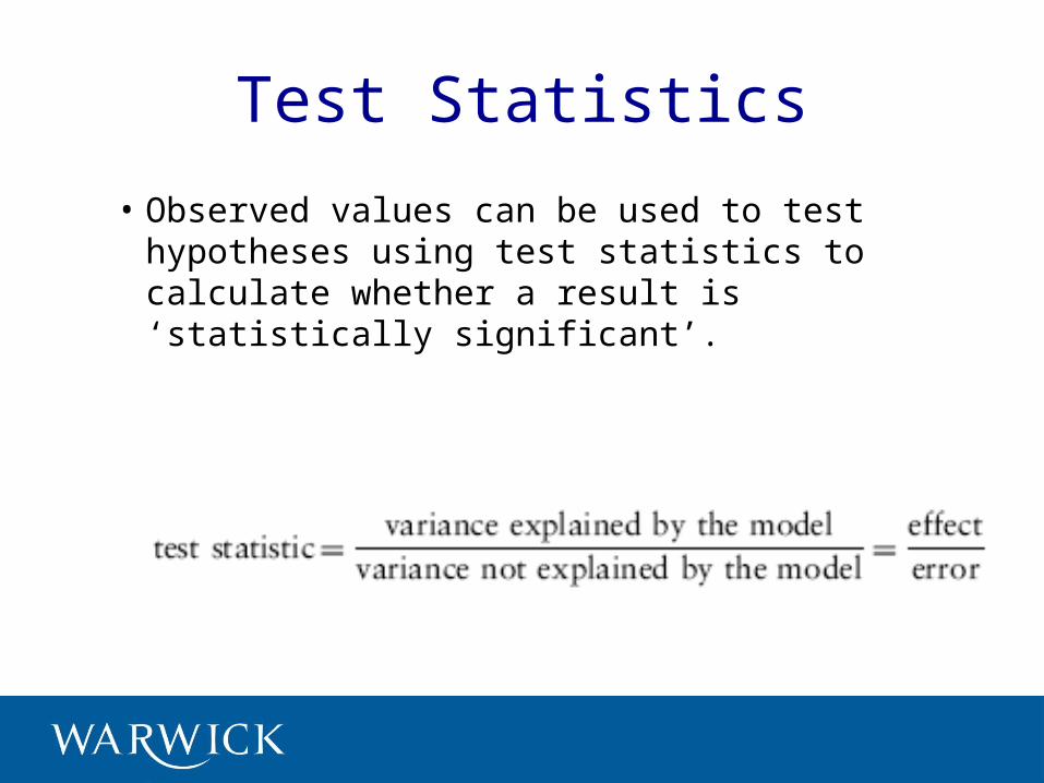
• Observed values can be used to test hypotheses using test statistics to calculate whether a result is ‘statistically significant’.

Normality (in statistics)• ‘Normality’ assumption = important.

• Underpins ‘parametric’ statistical tests.

• This is most commonly recognised from the bell shape of normal distribution.

Normal distribution• In general, the bell shape distribution has

the following characteristics

– The mean is located in the center of the distribution.

– The greater the distance from the mean, the lower the frequency of occurrence.

The assumed distribution of variables in the population

Normal distribution (approximately ‘bell-shaped’- underpinning assumption for parametric statistical tests)

No assumed distribution (as in non-parametric tests, which don't make the same assumptions about parameters but are consequently less effective at identifying underlying relationships than tests that do).

Type I and Type II Errors• Type I error

– occurs when we believe that there is a genuine effect in our population, when in fact there is not.

– The probability is the α-level (usually .05)

• Type II error– occurs when we believe that there is no effect

in the population when, in reality, there is.– The probability is the β-level (often .2)

Introducing Chi-square

Test

Categorical Data analysis• Today we are going to look at relationships between

categorical variables (i.e. gender, race, religion).• When both variables are categorical we cannot produce

means. • But we can construct contingency tables that show the

frequency with which cases fall into each combination of categories – i.e. ‘man’ and ‘Christian’– (we cannot do this with continuous variables such as age as

most people would fall into different categories and so the tables would be enormous and unmanageable).

Categorical Data analysis

• When we conduct statistical analysis of tabular data we are trying to work out whether there is any systematic relationship between the different variables being analyzed or whether cases are randomly distributed across the cells.

• Therefore the tests that we do compare what we find with what might be expected if there were no relationship – this is the null hypothesis.

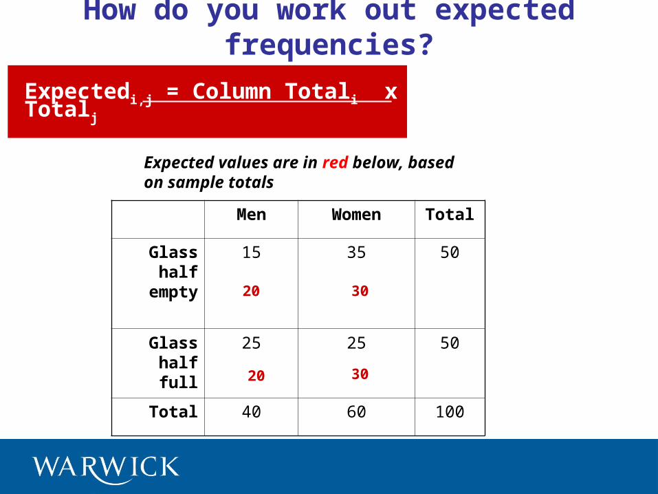
How do you work out expected frequencies?

Expectedi,j = Column Totali x Row Totalj

n

Men Women Total

Glass half empty

15 35 50

Glass half full

25 25 50

Total 40 60 100

20

20

30

30

Expected values are in red below, based on sample totals

Working out Chi-squareχ2 = (Observedij – Expectedij)2

Expectedij

= (15-20)2 + (25-20)2 + (35-30)2 + (25-30)2

20 20 30 30= (-5)2 + (5)2 + (5)2 + (-5)2

20 20 30 30= 1.25 + 1.25 + .833 + .833= 4.166

Men Women Total

Glass half empty

O: 15E: 20

O: 35E: 30

50

Glass half full

O: 25E: 20

O: 25E: 30

50

Total 40 60 100

Observed and Expected by cell:

This statistic can be checked against a distribution with known properties in a table (similarly to how you looked up z-scores).

However to look up a chi-square value we need to know the degrees of freedom (df).

Degrees of freedom in crosstabulations are calculated by (r-1)(c-1), where r is the number of rows and c is the number of columns. (i.e. the number of categories in each variable minus one and multiplied).

So here we have (2-1) (2-1) = 1 df.

A note on using Chi-square

• You can only use chi-square tests where each cell in the table has an expected value of at least 5. (Although where samples are larger it may be acceptable to have one cell with an expected frequency under 5). – If you violate this assumption the test loses power and may

not detect a genuine effect.• The categories must be discreet. No case should fall

into more than one category (i.e. you cannot think that the glass is half empty and half full).

And a note on presenting tables:1. When presenting tables you should always present percentages

(within the independent variable) – not frequencies (as these can be affected by the numbers of people in each independent category).

1. Percentages ‘tell the story’ more clearly. You do not need to give these to a million decimal places; 1 decimal place is usually adequate (and simpler to read).

Men Women

Glass Half Empty 37.5% 58.0%

Glass Half Full 62.5 42.0

Total (N)

100(40)

100(60)

Table 1: Outlook on life, by Gender

Thinking about Strength of Association

• Chi-square tells us whether there is a ‘significant’ association between two variables (or whether there exists an association that would be unlikely to be found by chance).

• However it does not tell us in a clear way how strong this association is since the size of chi-square depends in part on the sample size.

• We will look at two a different statistic that tells us about the strength of association: Namely, Cramer’s V.

Introducing Cramér’s V

– This is a Proportional Reduction in Error. (PRE) statistic that tells us the strength of associations in contingency tables.

– It also enables us to compare different associations and decide which is stronger.

– Another way of describing PRE is, how much better our prediction of the dependent variable will be if we know something about the independent variable.

PRE• PRE statistics range from 0 to ±1. Where (roughly

speaking):– values between 0 to ± 0.25 indicate a non-existent to weak

association

– values between ± 0.26 and ± 0.50 indicate moderate association;

– values between ± 0.51 and ± 0.75 indicate a moderate to strong association

– values between ± 0.76 and ± 1 indicate strong to perfect association.

• Note: the correlation coefficient also measures the strength of association between two variables on a scale between 0 and ± 1.

PG Stats Andy Field

Effect Sizes• An effect size is a standardized measure

of the size of an effect:– Standardized = comparable across studies– Not (as) reliant on the sample size– Allows people to objectively evaluate the

size of observed effect.

PG Stats Andy Field

Effect Size Measures

• r = .1, d = .2 (small effect):– the effect explains 1% of the total variance.

• r = .3, d = .5 (medium effect):– the effect accounts for 9% of the total variance.

• r = .5, d = .8 (large effect):– the effect accounts for 25% of the variance.

• Beware of these summaries of effect sizes’ meanings though:– The size of effect should be placed within the

research context.

Effect Size Measures

• There are several effect size measures that can be used:– Cohen’s d– Pearson’s r– Glass’ Δ– Hedges’ g– Odds Ratio/Risk rates

• Pearson’s r is a good intuitive measure– EXCEPT when group sizes are different …

Inferential Statistics: Correlation

Social Research Methods Dr Eric Jensen

43

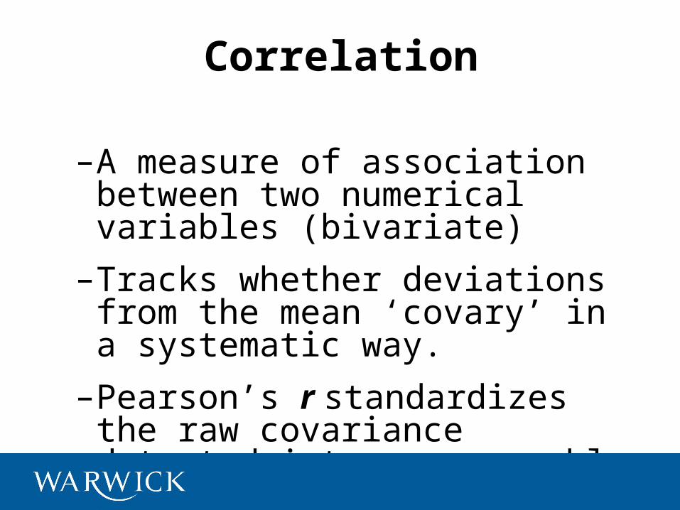
Correlation

–A measure of association between two numerical variables (bivariate)

–Tracks whether deviations from the mean ‘covary’ in a systematic way.

–Pearson’s r standardizes the raw covariance detected into a comparable correlation coefficient

–Only use with interval data!

Correlation– Note that correlation does not prove causality, but

merely covariance

– It is possible to have specious correlations, which do not actually tell us anything important

Correlation

Examples of correlation statements:

• “The more books that children read, the better their spelling”

- Consider the two numerical variables: ‘number of books’ and ‘spelling accuracy’scores the higher the number of books, the better the spelling therefore they are positively correlated

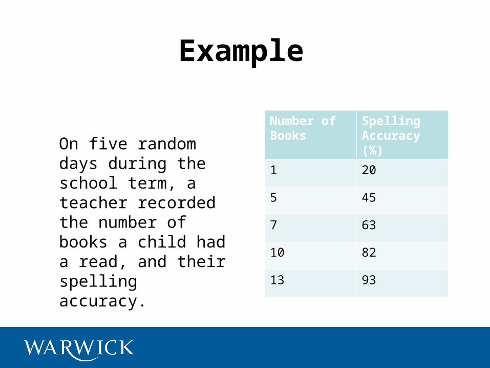
Example

Number of Books

Spelling Accuracy (%)

1 20

5 45

7 63

10 82

13 93

On five random days during the school term, a teacher recorded the number of books a child had a read, and their spelling accuracy.

Visual Representation

This shows there to be a somewhat linear relationship between the number of books read, and spelling accuracy

No. of Books

Measuring the relationship

• To measure the direction and the strength of the linear association between two numerical paired variables we use:

Pearson’s Sample Correlation Coefficient: r

– Note: When reporting results, use both r value and p value

Direction of Correlation• Can be either positive or negative

PositiveNegative

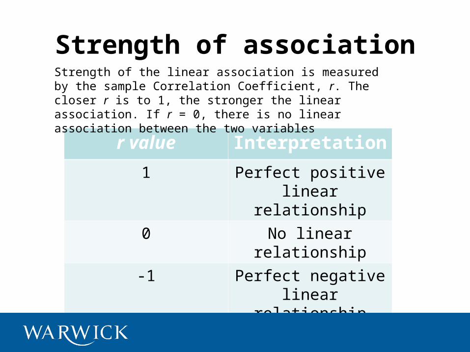
Strength of association

r value Interpretation

1 Perfect positive linear relationship

0 No linear relationship

-1 Perfect negative linear relationship

Strength of the linear association is measured by the sample Correlation Coefficient, r. The closer r is to 1, the stronger the linear association. If r = 0, there is no linear association between the two variables

Strength of association

Other Strengths of Associationr value Interpretation

0.9 Strong association

0.5 Moderate association

0.25 Weak association

Note: The same strength interpretations hold for negative values of r, only the direction of the association would change

Other Examples of Strengths of Association

Strength of the Association: r2

Coefficient of Determination: r2

• General Interpretation: The coefficient of determination tells the percent of the variation in the response variable that is explained by the model and the explanatory variable

• Around 0.1 = small effect• Around 0.3 = medium effect• Around 0.5 = large effect

Strength of the Association: r2

Interpretation of r2

Example: r2 = 0.36

• Interpretation: 36% of the variability in the accuracy of spelling is explained by the number of books read

Note: This means that 64% of the variation in the accuracy of spelling is not explained by this model using number of books

58

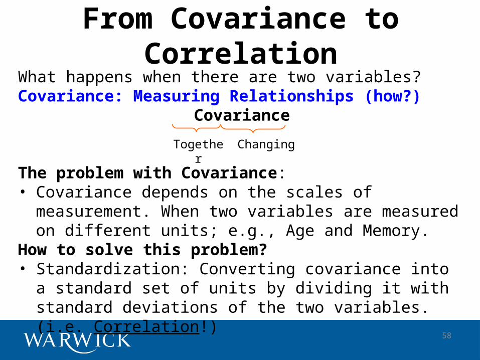
What happens when there are two variables? Covariance: Measuring Relationships (how?)

Covariance

The problem with Covariance:• Covariance depends on the scales of measurement.

When two variables are measured on different units; e.g., Age and Memory.

How to solve this problem?• Standardization: Converting covariance into a

standard set of units by dividing it with standard deviations of the two variables. (i.e. Correlation!)

Together Changing

From Covariance to Correlation

59

Correlation: Standardized covariance;What is the relationship between two (or

more) variables.

A measure of Linear relationship between variables.

Where r=Pearson’s Correlation Coefficient.

The value of r varies between -1 to +1 through 0.

Correlation

• Correlation matrix – correlates each variable against each variable including itself

Interpreting the output