Statistics of Extreme Events with Application to Climate

H. Abarbane1 S. Koonin H. Levine

G. MacDonald O. Rothaus

Accesion For

NTIS CRA&I OTIC T .. '\8 U, ,all:;o;l! • .:~d

JustiticOltion

o o

.. _--_ ..... -._ .......... --...... . ~--------, ...... -.--

By. --........................... ------.--........ -..

Availat)i'ily Code~

January 1992 ~--, AVdil ;j ,J 10;--

Sp~cjJI Dist

JSR-90-30S

Approved for public release; distribution WlIimIted.

This report was prtpIUed as an account of work sponsored by an agency of the United Slates Government. Neither the United Slates Government nor any agency thereof. nor any of their employees. makes any warranty. express or implied. or assumes any legal liability or raponsibility for the accuracy. completeness. or usefulness of any infonnalion. apparatus. product. or process disclosed. or represents that 115 use would notinfrtnge prtvately owned rights. Reference herein to any sped&c c:ornrnerdaI product. process. or service by trade name. trademark. manufacturer. or otherwise. does not necessartIy consIiIute or bTIp1y 115 endorsement. recornrnendalion. or favoring by the United Slates Government or any agency thereof. The views and opinions of authors expressed herein do not necasarily state or re8ect those of the United States Govanment or any agency thereof.

JASON The MITRE Corporation

7525 Coishire Drive Mclean, Vaginia 22102-3481

(703) 883-6997

REPORT DOCUMENTATION PAGE Fomt~

OM' No. 01Of.Q,U _.--. ........... ----01""-.. -10-... ' __ ,_._ ...... __ for--.....--...-cIIfftt-... ... _ ,-.... ... _ •• __ ........... COIIIIIfftIIt_--...._COll«ttOftof .......... -. - -~- ........ __ or..., __ of _ ___ of ... too_ ......... ~ .......... _ ......... IOW_ ........ ~ ___ ~ ~a..- ... ---. ms,...... o-........ IoIIteI ... a......-. V UlOl~JOI .... IO_OtItQof~......-' ..... IuCIOJet.'_~I'raIeftI1lJO&.GI •• W ........... DClOtCIJ.

1. AGINCY USI ONLY (L.a" tIIa") I Z. ll~lT DATE I I. lI~lT TV" AND DATES COVlllD January 10, 1992

4. TITLE AND SUlmu S. FUNDING NUMlIIlS

Statistics of Extreme Events with Application to Climate

PR - 8503Z 6. AUTHOl(S)

G. MacDonald, et al

7. ,.lPOlMING OlGANIZAnON NAME(S) AND ADDlESSeES) I. PElFOlMING DRGANIZA nON

The MITRE Corporation ll~lT NUMIEl

JASON Program Office A10 JSR-90-305 7525 Colshire Drive

McLean, VA 22102 t. SPONSDlING / MONITOllNG AGINCY NAME(S) AND ADDAESS(ES) 10. SPONSOllNG / MONITOllNG

AGINCY llflOaT NUMII.

Department of Energy JSR-90-305 Washington, DC 20585

11. SUPPLEMENTAl' NOTES

12 •• DlSTAIIUTIDN/AVAILAIlUT, STATEMENT 1 lb. DISTRIIUTION COOl

Distribution unlimited; open for public release.

11. AISTRACT (1IM.,mumlOOwonlll.l

The statistical theory of extreme events is applied to observed global average temperature records and to simplified models of climate. Both hands of records exhibit behavior in the tails of the distribution that would be expected from a random variable having a normal distribution. A simple nonlinear model of climate due to Lorenz is used to demonstrate that the physical dimensions of the underlying attractor, determined by applicable conservation laws, limits the range of extremes. These limits are not reached in either observed series or in more complex models of climate. The effect of a shift in mean on the frequency of extremes is discussed with special reference to possible thresholds for damage to climate variability.

14. SU.,ECT TEAMS

bernoulli trials, non-parametric order statistics, asymptotic distribution, lorenz 27-variable

17. SICUInY CLASWICAT10III ,a. SICUIllTY CLASSIfICATION 11. SlCUIUTY CLASS.ICATIOfII OF llPOllT OF THIS PAGE OF AlSTUCT

UNCLASSIFIED UNCLASSIFIED UNCLASSIFIED

1 S. NUMlll OF PAGIS

11. PRlCI CDOI

ZO. UMlTATIOfII Of AISTUCT

SAR Standard Form 198 (R.". l-l" __ ., ...... 'to '"""

Contents

1 INTRODUCTION 1

2 RETURN PERIOD 5

3 FREQUENCY OF EXCEEDANCES 9 3.1 Bernoulli Trials . . . . . . . . . . . . . . . . . . . . . . . . . . 9

4 NON-PARAMETRIC ORDER STATISTICS 11

5 APPLICATIONS OF ORDER STATISTICS TO GLOBAL AVERAGE TEMPERATURE 15

6 DISTRIBUTION OF EXTREMES 19

7 ASYMPTOTIC DISTRIBUTION OF EXTREMES FOR A NORMAL PROCESS 23 7.1 Applications of Asymptotic Theory of Extremes to a Climate

Model. . . . . . . . . . . . . . . . . . . . . . . . . . . . . .. 26 7.2 Physical Dimensions of an Attractor .............. 29 7.3 Extremes for a Climate Model with a Linear Increase in Tem-

perature . . . . . . . . . . . . . . . . . . . . . . . . . . . . .. 48 7.4 Distribution of Extremes for Global Average Temperature Record 50

8 EFFECT OF A SHIFT OF THE MEAN ON THE FRE-QUENCY OF EXTREMES 63

9 SUMMARY 69

III

1 INTRODUCTION

The social and economic costs associated with global warming will be

measured in terms of changes in the frequency and intensity of extreme events

such as droughts, floods, hurricanes, tidal surges, etc. Small changes in the

mean temperature are easily adjusted to, but successive years of drought or

a sequence of storms are much less easily handled even by advanced societies.

The capability to forecast the frequency and intensity of extreme events in

an altered atmosphere poses a great challenge.

In the statistical literature the large or small values assumed by a ran­

dom variable from a finite set of measurements are termed extreme values.

The variable of interest could be sea level, atmospheric temperature, pre­

cipitation, stream flow, etc. The largest and smallest value of the extremes

are often of most interest. However, other extremes such as the second or

third largest or smallest may be of interest. The extreme values are random

variables. For example, the minimum temperature in January in Bismarck,

North Dakota, exhibits random variations that are best described in terms

of probabilities.

The application of extreme value statistics is uncommon in the envi­

ronmental sciences except in the field of hydrology, where the concepts have

been used in designing dams. As noted in Levine et al. (1990), extreme value

theory has not received much attention in climate studies or in discussions of

greenhouse warming despite the obvious importance of large deviations from

1

the mean. The theory and applications are rarely treated in books on prob­

ability and statistics and almost never covered in university courses. If there

are references to the subject, it is generally to Gumbel's (1958) book which

has long been out of print. Cramer and Leadbetter (1967) and Leadbetter,

Lindgren and Rootzen (1982) provide an extensive treatment of extremes in

stationary sequences but focus primarily on certain of the difficult mathe­

matical issues related to extreme values. The statistics of extremes is closely

connected to order statistics which provides an approach to distribution free

or robust statistics (David, 1981). The present paper provides a review of

the theory with a number of applications that are related to climate change

ISSUes.

The applications are both to real data - time series of temperature

derived from various sources - and to results obtained from much simplified

computer models of climate. The latter application is primarily to provide an

illustration of how the problem of extremes can be approached, rather than

to give definite answers. Some of the examples could be extended to data

derived from large scale global circulation models (GCMs) of the atmosphere,

but since we do not have access to GCMs we have not done so.

Sections 2, 3 and 4 serve to introduce the nomenclature of order statis­

tics with a few elementary examples of the calculation of the probability of

extreme climatic events. In Section 5, results from order statistics are applied

to calculate the probability that the observed global average surface air tem­

perature records contain a trend. Unlike a previous analysis (Levine et aI.,

1990), no assumption is made as to the underlying statistical distribution.

2

Since 'extremes are rare events they can be approximated as independent

with negligible correlation. In accord with the earlier analysis (Levine et al.,

1990), order statistics indicate very high odds (l05 -106 to 1) in favor of the

hypothesis that the data records contain a linearly increasing trend in global

average surface air temperature.

Section 6 presents an introductory discussion of the distribution of ex­

tremes with no restricting assumptions as to the distribution of the parent

population. While general results can be obtained, detailed applications

require assumptions as to the underlying distribution. The theory is spe­

cialized in Section 7 to normal distributions. An application to the Lorenz

27-variable model of climate shows that the temperature values calculated

for the Lorenz model closely approximate normally distributed variates both

about the mean and in the tails (extremes) of the distribution for a rUll of

1000 years.

For a normally distributed random variable, the range (maximum mi­

nus minimum) increases without limit as the number, n, of variates selected

increases (as (In n)1/2). Section 7.2 provides an example where the phys­

ical dimension of the underlying attractor limits the growth in range with

time. This limit is not observed in model runs or in observed temperature

records (see Sections 7.3 and 7.4). Both model runs and observed tempera­

ture records from which a trend has been removed closely approximate nor­

mally distributed variates about the mean and in the tails of the distribution.

These results raise questions as to the predictability of climate.

The effect of a shift in mean on the frequency of extremes is discussed

3

in Section 8 with special reference to possible thresholds for damage due to

climate variability. Section 9 provides a brief summary of the major findings

of the report.

4

2 RETURN PERIOD

Engineers who design dams are interested in the time interval between

two discharges of a river, each of which is greater than or equal to a given

discharge. The probability p of a random variate X having a value greater

than x is

p = 1 - F(x) - 1 - i~ f(y) dy

F(x) - Pr(X ~ x)

where F(x) is the cumulative probability function and f(x) is the probability

density function. We are interested in the number of independent trials k

before the value x is exceeded. The variable k is an integer limited on the

left but not on the right, since the value of x may never be surpassed. The

probability that x is first exceeded at trial k is

since the event failed for the first k-l trials (Bernoulli trials). The mean for

k is simply

E [k] = IIp 1

- 1 - F(x) > 1.

The return period is defined by

1 T(x) == 1 - F(x)'

If an event has probability p, on the a.verage we have to make 1 I p trials in

order for the event to happen once.

5

The standard deviation for k is

which for a long return period becomes

1 0' '::!. v'2 (T - -).

2

The smaller the probability of an event, the larger the spread of the distribu-

tion. This general property lessens the usefulness of extremes in numerous

situations.

The cumulative probability W (k) that the event happens before or at

the kth trial is

W (k) = 1 - (1 _ p)k.

The probability that the event will happen before its return period T is

W(T) _ 1 - (1 _ .!.)T T

~ 1 - ~ = 0.6231. e

H the value to be exceeded, x, is large and the return period long, say

greater than 10, then the cumulative probability W(k) can be approximated

by k

W(k) '::!. 1 - exp( - T).

In hydrology the return period is usually measured in years. For exam­

ple, a design engineer may wish to have a high probability (0.95) that an

event does not happen in N years. The return period T for the design is then

6

approximately N

T= l-W

80 that in order to have a probability of 1 in 20 that the event does not

happen in 10 years requires the design to have a much larger return period

of 200 years.

These simple considerations illustrate certain features of the statistics of

extremes. Under the assumption that the events are independent, results can

be obtained that are free of any assumption with respect to the underlying

distribution. The assumption of independence might appear to be highly

restrictive. For dependent variables, their correlation as a function of time

difference or lag is a partial measure of their dependence. Many of the results

derived for independent variables apply to dependent variables provided that

the correlation decreases rapidly enough with lag (Leadbetter, Lindgren and

Rootzen, 1983). The basic reason for applicability of results obtained from

the theory of independent events to correlated series is that extreme events

are rare. Rare events are expected to be separated by long time intervals

80 that the effects of correlation are negligible. If the correlation function

decays at least as fast as 1/ In n where n is the time, then the effects of

the correlation can be neglected as is discussed by Leadbetter, Lindgren and

Rootzen (1983).

7

3 FREQUENCY OF EXCEEDANCES

3.1 Bernoulli Trials

The statistics of Bernoulli trials can easily be applied to extreme events.

The probability that during the next n years the maximum July temperature

in Washington, D.C., will exceed 105°F exactly k times is

where p, estimated on past observations, is the probability that the maximum

July temperature will not exceed 105°F and where

n n! ( k ) = (n - k)! k!

is the binomial coefficient. The probability of exceeding 105°F in Washington

is about a 1 in 20- year event, p = 0.95. In the next decade, provided that

there is no upward or downward trend in temperatures, the probability that

the maximum July temperature will not exceed 105°F is

or there is a 40 percent chance that the maximum July temperature will

exceed 105°F in the period 1990-1999.

The probability that during the next ten years there will be fewer than

three years for which the maximum temperature for July exceeds 105°F can

9

also be calculated. There are only three ways that the number of exceedances

of 105°F cannot be greater than two - namely when the number is zero, one

or two. The probability of these mutually exclusive events is the sum of the

probabilities of each

Po + PI + P2 = (1~) (0.95)10 (0.05)0 + ( 110

) (0.95)9 (0.05)

+ (1:) (0.95)8 (0.05)2 = 0.9885.

The probability of the maximum July temperature in Washington in the

next decade exceeding 105°F three or more times is only 1 in a 100. H in the

next decade the temperature does exceed 105°F in July three or more times,

the hypothesis that there is no upward trend in the temperature should be

reexamined.

The number of exceedances depends on the interval over which the ob­

servations are made. From the results of the above example we can calculate

the probability that over the next century every decade will have no more

than two Julys in which the maximum temperature exceeds 105°F. With a

shift in time scale the probability is

P = ( 100 ) (0.9885)10 (1 - 0.9885)0 - 0.89.

10

4 NON-PARAMETRIC ORDER STATIS­TICS

The need to estimate the probability Pm of the mth ranked observation

can be avoided by using past observations to determine the exceedances in

future trials. Let n denote the number of past observations, N the number

of future observations, m the rank of the ordered past observation and k

the number of exceedances of the mth ranked observation in N future trials.

The probability of observing in N trials, k exceedances of the mth ranked

observation seen in n trials is:

P(k;n,m,N) ( N )( n )m fl pN-k (1 _ p)k pn-m (1 _ p)m-ldp k m Jo

( : )( ~ )m

(N + n) ( N + n - 1 ) m+k-l

since the integral is a special case of the Beta integral

For the largest value, m = 1, the probability of k exceedances is

nN!(N + n - k -I)! P(kj n, I,N) = (N _ k)! (N + n) (N + n - 1)'"

The probability that the maximum value observed in n trials is not exceeded

in N future trials is n

P(O;n,I,N) = N ' +n

11

and there is 0.5 probability that the maximum is not exceeded in an equal

number, N = n, of future trials. The calculation of the probabilities for the

exceedance of the largest value is aided by the recursion relation

(N + 1 - k) P(k+l;n,I,N)= (N+n-k) P(k;n,I,N).

The probability that all values in N future trials will exceed the largest

value observed in the first n trials is small. For the case N = n, this proba­

bility is (N!)2

P(N; N, 1, n) = (2N)!

which for N = 6 is 0.00108.

The various moments of the distribution function can be obtained from

properties of the hypergeometric function (Gumbel, 1954). The mean number

of exceedances is

N

E (n,m,N) - L k P(k;n,m,N) k=l

- mN/(n + 1).

Similarly, the variance of the estimate of the number of exceedances is

2( N)_m(n-m+l)N(N+n+l) u n,m, - (n+l)2(n+2) .

The variance increases with the number, N, of future trials and decreases

with the number of past observations used to set up the statistics. The

variance for the number of exceedances of the maximum is

2 nN(N+n+l) u (n,l,N) = (n+ 1)2 (n+2)"

12

The variance of the estimate for the median, m = nil, n odd, is

2( n+l N)=N(N+n+l) u n, 2 ' 4{n + 2)

so that the ratio of the variance of the estimated number of exceedances of

the maximum to the number of exceedances of the median is

u2(n, 1, N) _ 4n u2(N, nr,N) - (n + 1)2·

In one sense, the extremes are more reliable than the median since the vari­

ance of the number of exceedances of the median is about ~n as large as the

variance for the maximum. In the limit of large N with N = m the mean

and the variance take on simple forms

E[k] ~ m

and

The mean number of exceedances over the mth largest value is equal to

the rank m itself. The distribution is then similar to a Poisson distribution

for integers. However, the variance is twice that of a Poisson distribution.

The probability distribution of exceedances in this case is independent of the

distribution of the random variable X. It does depend on the assumption that

the observations are independent. The lack of dependence on the distribution

is an a.ttractive feature of the theory, since the distribution may be known

in the vicinity of the median but there will, in most cases, be very few

observations with regard to extreme values.

13

5 APPLICATIONS OF ORDER STATIS­TICS TO GLOBAL AVERAGE TEMPER­ATURE

A 109-year record of the annual global average temperature of the at­

mosphere has been determined by Hansen and Lebedetf (1987, 1988) (see

Figure 1). The data have been normalized to zero mean. The maximum

temperature for the 100-year period 1880-1979 is 0.2°C, observed in 1954.

The probability of one or more exceedances of the maximum of this 100-year

record in the nine-year period 1980-1988 is

100 P (> 1; 100,1,9) = 1 - 109 = 0.083

if the average temperature can be taken as an independent trial and there

is no trend. The expected number of exceedances is E(100, 1,9) = 9/100 =

0.089 with a variance of (7'2(100,1,9) = 0.095. In fact there were five ex­

ceedances: 1988, 1981, 1987, 1983 and 1980. The probability under the

independence assumption of five exceedances is

P (5;100,1,9) = 1.03 x 10-6•

The observed five exceedances strongly contradict the assumption of inde­

pendence and provide support for the hypothesis that there is an increasing

trend in the annual global average surface temperature.

H a linear trend with a least square slopes of 0.55° per century is removed

the maximum residual in the first 100 years is 0.28°C in 1926. There are no

exceedances for the years 1980-1988 in the residual as would be expected from

15

0.60 r-----------------------------..

-0.80 &.... ____ ..... ____ -'-____ ...L. ____ -'-____ --'_---I 1880 1900 1920 1940 1960

Date

Figure 1. Variations of global average temperature. The solid curve is a filtered version corresponding to a five-year running average (after Hansen and Lebedeff, 1987; 1988).

16

1980

Table 1

Expected Number of Exceedances in Six-Year Runs of Global Annual Average Temperature and Observed Exceedances in 17

Six-Year Runs

Observed Number of Exceedances

Number of in Residual Exceedances k Expected after Removal of Maximum Probability Number of Observed Number of Linear

Value of k Exceedances of Exceedances Trend

0 0.5 8.5 0 2 1 0.273 4.64 1 3 2 0.136 2.31 1 3 3 0.061 1.03 0 4 4 0.027 0.46 2 2 5 0.006 0.11 1 1 6 0.001 0.02 12 2

the probability distribution for the maximum. In terms of odds, the ratio of

the probability of the observations containing a trend to the probability that

the temperatures are independent, identically distributed random variables

IS

0.917 =8.9xI05 •

1.03 x 10-6

As a further example of the use of the probability distribution, the 108-

year record, 1980-1987, is divided into 18 consecutive six-year segments. The

maximum value in the first six-year period, 1880-1885 is - 0.37°C. The num­

ber of exceedances in each of the subsequent six-year segments is tabulated

in Table 1 along with the number obtained for the probability distribution.

17

The expected number of exceedances in any six-year period is

E (6,1,6) = 6/7 = 0.86

with a standard deviation of

iT = 1.09.

Clearly the number of six-year runs with all six values in excess of the maxi­

mum for the first six-year segmeut is much larger, 16, than would be expected

from a sequence of independent trials. The probability of obtaining 12 seg­

ments out of 17 in which all the values are in excess is

17! (12 5 -32 12! 5! 0.00108) (1 - 0.00108) = 1.5 x 10 .

Table 1 also tabulates the observed distribution of exceedance for the resid-

uals after a linear trend has been removed. The observed distribution still

differs from the calculated one. However, the probability of obtaining two

segments in which all six values are greater than the maximum observed in

the first six-years while small, 1.5 x 10\ is much larger than the probability

of obtaining 12 such sequences.

Levine et. al (1990) calculated that the odds for a linear trend in the

data were 1.7 x 105 to one. In that analysis, the correlation between annual

temperature was explicitly taken into account through the use of the full

covariance matrix in the least squares analysis but the analysis was based

on the assumption that the global average temperatures were normally dis­

tributed. The analysis presented above supports the hypothesis of a trend by

similar odds, but is based on the assumption of independent trials without

any assumption on the underlying statistical distribution.

18

6 DISTRIBUTION OF EXTREMES

The above analysis provides information with respect to the number of

observations that would exceed the mth largest value of n initial observations.

The analysis provides no information on the value that would exceed the

observed extremes. Such information requires that the underlying probability

distribution, F(x), be known. As illustrated above, some of the analysis of

the frequency of exceedances can be carried out without assumptions with

respect to the underlying distribution of the random variable. The exact

form of the distribution is generally not known, but an asymptotic theory

that covers a wide variety of initial distribution has been developed (Cramer,

1946, Gumbel, 1958).

As before, let k denote the kth value from the top of a sample of n

observations. The probability density g(Xj n, k) for the kth value is equal to

the probability that among n samples n - k are less than x, and k - 1 are

greater than x while the remaining value falls between x and x + dx

g(Xj n, k) = n( ~ = ~ )[F(x),,-k (1 - F(x))k-l]f(x)dx

where F(x) is the probability distribution function and f(x) is the density

distribution function. For the maximum value k = 1 and

g(xjn, 1) = [F(x)]" dx.

For a population having a normal distribution with zero mean and unit vari-

ance

F(x) = ~1% e- t '/2 dt. v211' -00

19

The dependence of the maximum value on the number of observations from

a series of independent trials drawn from a normal population is illustrated

in Figure 2. For a sample of ten, the maximum has a 0.05 probability of

exceeding 2.57 standard deviations; for a sample of 1000, the maximum will

exceed 3.89 standard deviations one in twenty times.

20

••••• , ,. •• ~

~ . •• •

0.9 •• , , • •• I • • ,

• I • • • I 0.8 • I • • • • I I • • I • 0.7 • I • I • • • ,

• , • •

0.6 • I ,

• • • ~ • , , i • • • , ,

0.5 • • • £ • , • , • , •

0.4 n - 10'- n - 1000, ! n - 10.000 • • , I • • • 0.3 • , ,

• , • • I • • , • • , 0.2 • , • • • , • I • • • I • , • 0.1 •• I •

•• I I •• • •• ~ , 0 •••

0 2 3 4 5

X Measured In Sid.

Figure 2. Variations of the probability of the maximum of n independent trials with n. The distribution has zero mean and unit variance.

21

7 ASYMPTOTIC DISTRIBUTION OF EX­TREMES FOR A NORMAL PROCESS

The general asymptotic theory of the distribution of extremes deals with

the conditions under which

approaches a limiting distribution G(x) where a" and b" are suitable normal­

izing constants and

The theory states that every distribution G, has, up to scale and location

changes, one of the following parametric forms commonly called the Three

Extreme Value distributions:

Type I: oo<x<oo G(x) = exp( _e-r )

Type II: x>O G(x) = exp( _x-a); Q > 0 x~O G(x) = 0

Type III: x <0 G(x) = exp( -( _x)O); Q > 0 x>O =1

(Leadbetter, Lindgren and Rootzen, 1983). The normal distribution, unlim­

ited on the left and right, falls into the Type I domain of attraction. The

density distribution for the kth ordered value becomes

which is illustrated in Figure 3 for k = 1, 2, 3.

For a normal distribution with zero mean and unit variance, if x is the

23

1.4

, .. , , , \ 3

1.2 , , , , , • , • , , , • , • , • , • ,

i • , , , ~ 0.8 • • ,

I • • • •

0.6 I ci: • • • • •

0.4 •

figure 3. The probability density function for the double exponential.

24

kth value from the top, then { is

The normalizing constants can be obtained by a complex calculation.

The solution for x when n is large can be obtained by partial integration

leading to

With bounded {, x is given by

1/2 In In n + In 411" In { 1 x = (2 In n) - 2(2 In n)1/2 - (2 in n)1/2 + O( in n)·

For the general form of the normal distribution with arbitrary mean m and

variance (T2, the form for Mn = x is asymptotically

_ 112 In In n + In 411" (T v X - m + 0'(2 In n) - 0' 2(2 in n)1/2 + (2 In n)1/2

where v is a random variable having the frequency function

The expression for the kth value from the bottom is given by a similar ex-

pression with opposite sign for all terms but the mean, m.

The expected value Cor the kth value from the top is

E[ . k] = (2 I )1/2 _ In In n + In 411" + 2(81 - C) 0(_1_)) x,n, m+O' nn (2/nn)1/2 + Inn

with variance D2

0'2 D2(x· n k) = --:---

" 2 In n (n-2 _ 82) + 0 (_1 ) 6 In2 n

25

---------------------------- ._----_.> .. > ......... > ......... .

where C is Euler's constant, C=0.57722 ... ,

1 +k-1

1 + (k -1)2'

Similar expressions can be calculated for the difference between the kth max­

imum and kth minimum values of the n independent trials drawn from a

normal population.

E[ _ . k] = (4 In n -In In n -In 411" - 2(51 - C) 0(_1_»)" x 1/,n, (1 {2 In n)1/2 + Inn

(12 11"2 1 D2[x -1/; n, k] = -(- - 52) + 0(-).

In n 6 In2 n

The dependence of the range on the number of observations is indicated

in Figure 4. The three standard deviation bounds are also shown. For a

normal population of a 1000 variables there is about 1 in a 100 probability

that the maximum range will exceed eight standard deviations. The expected

value for the maximum of normal population is shown in Figure 5.

7.1 Applications of Asymptotic Theory of Extremes to a Climate Model

The variation of global average annual temperature depicted in Figure 1

shows irregular behavior with a non-vanishing correlation function for lags

up to the length of the record and continuous power spectrum with abun­

dant energy at low frequencies (Levine et.al, 1990). The irregular behavior,

characteristic of chaotic systems, also shows clearly in complex models of the

26

10~----------~-----------r----------~----------~~--------~

6

-2

-4

-------_._----------------------­.. -------

-- -----------­...... -----

-6 ~----------~----------~--------~~--------~----------~ o 200 400 600 800

Number of Observations

Figure 4. Variations of the maximum expected range for a random variate drawn from a normal population as a function of the number of observations. The distribution has zero mean and unit variance. The three standard deviations from the expected value are also shown.

27

1000

3£" ;:

4 r----------,----------~----------~----------~--------~

----------------- --------------, 3.5

------ .-------_ .. -­-----.---.-----.-_ . . -,. ,,"

" " " , , , , , , , , , • ,

'.5 I , , I I , u-__________ ~ ____________ ~ __________ ~ ____________ ~ __________ ~

o 200 400 600 800

Number of Observations

Figure 5. Variation in expected maximum value of an observation drawn from a normal population with zero mean and unit variance as a function of the number of observations. The three standard deviations from the expected value are also shown.

28

'000

atmosphere such as General Circulation Models, which contain about 100,000

coupled nonlinear equations, and also in the simplest models. Lorenz (1984a)

has developed a low-order model in 27 variables that has been analyzed in

some detail by Levine et a1.,(1990). The physical variables include the mix­

ing ratios of water vapor and liquid water as well as temperature, pressure

and the usual dynamic variables. In the Lorenz model, the atmosphere and

ocean exchange heat and water through evaporation and precipitation. The

model also produces clouds, which reflect incoming solar radiation, while

both phases of water absorb and re-emit infrared radiation.

For a WOO-year run for the global average annual temperature, the ob­

served standard deviation was 0.3583°C. The data scaled to unit variance and

zero mean are shown in Figure 6. The observed maximum value is 3.407. The

probability of obtaining this value with 1000 values is 0.712, or a probability

of 0.29 that 3.4 would be exceeded in a WOO-year run of independent trials

drawn from a normal population. The distribution of temperature deviations

about the mean approximate a normal distribution as illustrated in Figure 7.

The variation of range with the number of observations is shown in Figure 8.

The variation closely follows the expected value of the range drawn from a

normal population.

7.2 Physical Dimensions of an Attractor

For a truly random, non-deterministic process, such as a variate drawn

from a distribution unlimited on the left and right, the range will grow with

29

4

3

2

0 0

~ 0 11

~ E ~

-1

-2

-3

-4 0 200 400 600 800 1000

Time (Years)

Figure 6. Variation of global-mean. annual-mean. sea-level air temperature for 1000 years in a numerical solution to the Lorenz 27-variable model of the atmosphere. Data are rated to unit variance and zero mean.

30

140r--------------------------------------------------------,

! § Z

120

100

80

60

40

20

oL-__ ~ .. ~_L~~~~_L~~~~_L~~~~_L~~~ __ ~

-4 -3 -2 -1 o 2 3

Deviations (Unit Variance)

Figure 1. Distribution of global-mean, annual average temperatures for 1000 years of the Lorenz model.

31

4

• ,4 ; Q 0,

7

- -f----6 - ---1-.'- ....

,,~

5 - ~ I -Q) I u

.Iii 4 J ~ I ~ I 2-

~ GI 3 c:a

~

2

1 ~

0 I I I I 0 200 400 600 800 1000

Time (Years)

Figure 8. The variation with time of the range of global-mean, annual average temperature for the Lorenz model. The dotted curve gives the expected value for the range for samples drawn from a normal population.

32

the number of variates selected at a rate approximately

For a time series n, the number of variates equals the number of time units.

In a deterministic system governed by a set of coupled nonlinear differen­

tial equations, one would expect that the embodied conservation equations

would set limits to the maximum growth of any state variable. In terms of the

language of nonlinear dynamical systems, the -governing attractor has finite

physical dimensions. In this context we are speaking of the physical dimen­

sions of the attractor as contrasted to the usual embedding dimensions which

constitute a measure of the denseness of the set making up the attractor.

In the limit of large times, the range of random variables grows without

bound but very slowly as (In n )1/2. For deterministic systems, the growth, as

noted above, should be limited at a large enough n. For the Lorenz system,

it is apparent that the limit has not been reached in 1000 years (see Figure 8).

A general problem is that of determining the limits to the range of a

particular variable and the time required to explore the far reaches of the

attractor. It would appear that these are difficult issues, particularly for a

system as complex as the 27-variable Lorenz system.

In order to further examine the time required for the Lorenz 27-variable

model to explore the outer regions of the attractor, the model was run for

10,000 years. The results are shown in Figure 9. It would appear that

the times to attain the outer reaches of the attractor are on the order of

5,000 years. To distinguish between a random process with the events drawn

from a normal population and a deterministic Lorenz system by examining

33

Range for Gaussian Distribution 1.60

Dew Point Temperature 7.00 .... -_._------­

-~-~-~¥~-~-~-~.~ - - - - -:-,:-:::-:::-.:;-.:;4 Sea Surface Temperature

6.40 ~:""-----'"1

5.80

:1 5.20

4.60 :I j

1 4.00

! 3.40

2.80

2.20

1.60

1.00 0 2000 4000 6000 8000

itme in Years

Figure 9. The variation with time of the range of the globally averaged values of surface atmosphere temperature. sea surface temperatures and dew point temperature. The values are averaged owr a month and reported each year. The model is the Lorenz 27 -variable model. The data are normalized to zero mean and unit variance. The heavy curve is the expected value of the range for a sample drawn from a normal population.

34

100000

------------------------------------------------------------------------------------- -

the tails of the distribution one would need to select on the order of 104

values. This observation suggests that before asymptotic behavior is reached

by a dynamical system, transients of considerable duration can occur. Also

shown in Figure 9 is the variation of the range of sea surface temperature

and dew point temperature as calculated in the model. The tails of trails of

the distribution of the parameters differ from that of a normal population,

but very long times, on the order of 104 years, are required to reach the

outer edges of the attractor. There is, of course, no guarantee that in any

single integration the system will reach the boundary of the attractor. A

further consideration is the random roundoff noise generated in the computer

integration. This noise will cause the calculated range to mimic a random

variable.

In a simple system, again one proposed by Lorenz (1984b), it does ap­

pear possible to obtain bounds on the maximum dimensions of the attractor.

Lorenz (1984b) labels the following set of three coupled nonlinear equations

as the simplest possible general circulation model:

dX - y2 _ Z2 - aX + aF dt -dY

XY -bXZ - Y +G dt -dZ

bXY +XZ -Z. dt

-

The variable X represents the strength of the large-scale westerly-wind cur­

rent or the geostrophically equivalent equatorial-pole temperature gradient,

while Y and Z are the strengths of the cosine and sine phases of a chain of

superposed waves (Lorenz, 1984b). The quadratic terms containing b rep­

resent the translation of the waves by the western current. The remaining

35

quadratic terms represent a continual transfer of energy, except when X is

negative, from the westerly flow to the waves.

The principal external driving force, the contrast between equatorial

and pole heating, acts directly on the zonal flow X and is represented by a

F. A secondary driving force, dependent on the difference between oceans

and continents, enters the equations through G.

A section of the attractor for the Lorenz 84 model is displayed in Figure 10,

which shows the range for the Z variable projected onto a plane including

the Z axis and at an angle 8 to the X axis. The motion is centered about

Z = 0 but otherwise offset in X and Y.

We treat X, Y and Z, as coordinates in three-dimensional phase space.

A rate of change of energy equation follows from the governing set by multi­

plying.each by 2X,2Y, and 2Z, respectively and summing

where R2 = X 2 + y2 + Z2 can be interpreted as the total energy - the sum

of the kinetic, potential and internal energies. The right-hand side of the

equation for Ii:" vanishes on an ellipsoid

a(X _ F/2)'l + (Y _ G/2)'l + Z2 = aF'l: G2

•

The rate of change of energy outside the ellipsoid is negative. This implies

that for any sphere centered on the origin in state space enclosing the el­

lipsoid, orbits passing through points outside the sphere will eventually pass

through the sphere and remain inside. The ellipsoid is centered at (F /2, G /2,

36

2.1

1.8

1.5

1.2

0.9

0.6

0.3

c- 0.0 N

-0.3

-0.6

-0.9

-1.2

-1.5

-1.8

-2.1~--~ ____ ~ __ ~L-__ -L ____ ~ __ ~~ __ ~ ____ ~ ____ L-__ ~ ____ -I

-3.5 -3.0 -2.5 -2.0 -1.5 -1.0 -0.5 -0.0 0.5 1.0 1.5

x(n) c~s(t'J) + YIn) ::;:n(t'J)

Figure 10. A section of the attractor for the Lorenz 3-variable model at a plane containing the z axis and at an angle of 1170 to the x axis. The parameters for the model are given in Table 2.

37

2.0

Table 2

Maxima and Range for Variables Defined in Lorenz Lowest Order Central Circulation Model

(F=8.0, G=1.0, a=0.25, b=4)

Variable Maximum Minimum

X 12.24 -0.12 Y 3.06 -1.06 Z 2.06 -2.06

0) with the corresponding major axes (( aF:!G2 )1/2, (aF2tG2 )1/2, ( aF2t

G2 )1/2).

The maxima and minima for the state variables are given in Table 2 for

initial conditions lying within the ellipsoid and for specific values of the con­

stants F, G and a. For initial conditions lying within the ellipsoid defined by

d:'2 = 0, aU orbits would be expected to remain within the ellipsoid, except

for small inertial excursions, in the absence of noise. The ellipsoid provides

the limits for values that can be taken on by the state variables. The con­

stant b does not enter into the equation for the critical energy surface since

b defines the strength by which the waves are carried by the zonal westerly

current and does not alter the energy of the system.

The above analysis provides bounds on the maxima, minima and range

attained by the state variables but provides no estimate of the average time

required for a state variable to reach the boundary of the attractor. The only

time scale within the systems of equations is determined by the constant a,

the inverse of the decay time for the zonal current. Lorenz (1984b) assumes

38

a decay time for the zonal current of 20 days by selecting a=0.25 and taking

5 days as the unit time.

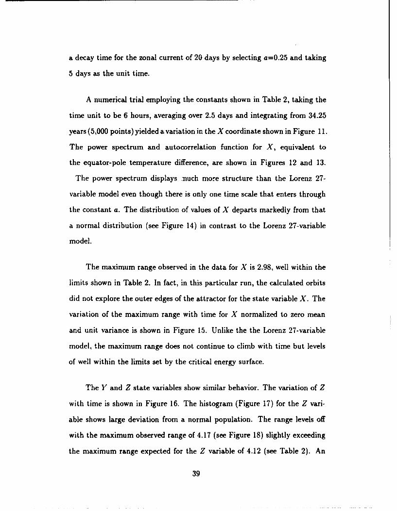
A numerical trial employing the constants shown in Table 2, taking the

time unit to be 6 hours, averaging over 2.5 days and integrating from 34.25

years (5,000 points) yielded a variation in the X coordinate shown in Figure 11.

The power spectrum and autocorrelation function for X, equivalent to

the equator-pole temperature difference, are shown in Figures 12 and 13.

The power spectrum displays .nuch mo!"e structure than the Lorenz 27-

variable model even though there is only one time scale that enters through

the constant a. The distribution of values of X departs markedly from that

a normal distribution (see Figure 14) in contrast to the Lorenz 27-variable

model.

The maximum range observed in the data for X is 2.98, well within the

limits shown in Table 2. In fact, in this particular run, the calculated orbits

did not explore the outer edges of the attractor for the state variable X. The

variation of the maximum range with time for X normalized to zero mean

and unit variance is shown in Figure 15. Unlike the the Lorenz 27-variable

model, the maximum range does not continue to climb with time but levels

of well within the limits set by the critical energy surface.

The Y and Z state variables show similar behavior. The variation of Z

with time is shown in Figure 16. The histogram (Figure 17) for the Z vari­

able shows large deviation from a normal population. The range levels off

with the maximum observed range of 4.17 (see Figure 18) slightly exceeding

the maximum range expected for the Z variable of 4.12 (see Table 2). An

39

2.5~---------------------------------------------------------,

2

1.5

x

0.5

o

-0.5

-lLo-----------1-oLoo-----------2~00~0----------3-0~0-0----------4-0~0-O--------~5~000

Time (unit = 2.5 days)

figure 11. Variation of the Lorenz 3-variable model X coordinate (X is the equatorial-pole temperature gradient) with time for 12.500 days.

40

10'r-------------------------------------------------------------__

10-·~-------4--------~------~--------~------~--------~------~ o 0.2 0.4 0.6 0.8 1.2

FreQuency (Cycles Per Day)

figure 12. Power spectrum for state variable X in Lorenz 3-variable model. The data are normalized to zero mean and unit variance.

41

1.4

0.8

0.6

0.4

0.2

a

-0.2

-0.4

-0.6~----------~----------~----------~----------~----------~ o 50 100 150 200 250

Figure 13. Autocorrelation junction for state variable X in Lorenz 3-variable model. The data are normalized to zero mean and unit variance.

42

500

450 ~

400 ~

350 ~

300 --250 -200 -150 -100 -50 -o -3

-

r-

r--

---r

-2 -1

r-r--

r-

r--~ -

--

-.....-

-r--

I In o 2

Figure 14. The distribution of value for the X state variable in the Lorenz 3-variable model. The data have been normalized to zero mean and unit variance.

43

3

8~----------~----------~----------~----------~----------_

7

6

5

& .! 4

3

2

o~----------~----------~----------~----------~----------~ o 1000 2000 3000 4000

TIn1e (Unit - 2.5 days)

figure 15. Variation of the range of the state variable X in the Lorenz 3-variable model. The data are nonnaJized to zero mean and unit variance. The dotted line is the range expected for values chosen from a normal population with unit variance and zero mean.

44

5000

3~----------~----------~----------~-----------r----------~

2

z

-3~----------~--------~~--------~----------~----------~ o 1000 2000 3000 4000 5000

Tune (Unit - 2.5 Days)

Figure 16. Variation of the Z state variable with time for the Lorenz 3-variable model. The unit of time is 2.5 days.

45

· ;

500

450 "'""

400 -350 ~

300 --250 --200 -150 -100 -

50 -o -3

iA

I

.--

m--2

I I T .--

I-

r-- -:-- I--

.--

.--

'-

.--

I -1 o

Figure 17. Histogram for the Z state variable in the Lorenz 1984 model.

46

T

-------

I- --

'-

-I 2 3

8r-----------T-----------,-----------~----------~----------~

7

6

5

3

2

o~----------~----------~----------~----------~----------~ o 1000 2000 3000 4000

Time (Unit - 2.5 Days)

Figure 18. Range for the Z state variable in the Lorenz 1984 model. Data have been normalized to unit variance and ZE!"O mean. The curve represents expected range for a normaJly distributed var:able.

47

5000

Ai «-' 0;

observation of a value for the range slightly in excess of the ma.ximum pre­

dicted range is not unexpected, since inertia will carry the the orbit outward

before the- inward pull of the attractor brings the orbit back within the limits

of the critical energy surface.

The above example illustrates that it is possible to predict the maximum

range of variables in a complex nonlinear system provided the equations are

known. The limitation to the range of values which variables can assume

likely comes from the conservation equations governing the motion. The

time scale over which the maximum value may be attained is not determined

by the above analysis.

7.3 Extremes for a Climate Model with a Linear In­crease in Temperat ure

Levine etal., (1990) describe a version of the Lorenz 27~variable model

in which the solar insolation is increased linearly with time leading to an

increase of global temperature of 10° over a 1000~year period. The resulting

temperature record is shown in Figure 19. The calculated variance is 9.24,

which can be broken down into the part due to the linear increase and (72,

the variance about the linearly increasing mean.

N 2b2 Var ~ __ +(72

12 (72 _ 0.235

where N is the number of years and b is the rate of temperature increase.

48

8

6

4

0 2 0

S i 0

~ -2

-4

-6

-8 0 200 400 600 800

Tme (Years)

Figure 19. Global average temperature for Lorenz 27-variable model of the atmosphere in which the parameter corresponding to the insolation is increased linearly in time to provide an approximately tOO( increase in temperature over 1000 years.

49

1000

The residual temperature curve after removing a trend by least squares

is shown in Figure 20 with a distribution of the residuals approximating a

norm"'} distribution (see Figure 21). The maximum range after 1000 years

for the residuals approximates the range expected by drawing variates from a

normal population (see Figure 22). The removal of a trend before analyzing

for extremes is a useful way of examining records of global average, surface air

temperature records. There is a high probability that these records contain

a linear trend (Levine et a1. 1990).

7.4 Distribution of Extremes for Global Average Tem­perature Record

Our final example of an application of extreme value theory is to an an-

nual average, global surface air temperature record. Three research groups

(Jones, 1988; Hansen and Lebedeff, 1987, 1988; and Vinnikow et aI., 1990)

Ita\,(' produced similar analyses of hemispheric surface temperature variations

from somewhat differing initial data sets. The longest of the data sets is that

of Jones (1988) and we will use it in the analysis. An analysis of the Hansen­

Lebedeff (1987,1988) series (see Figure 1) produced results similar to those

obtained from the Jones record. The Jones global average temperature vari­

ation is shown in Figure 23, which can be compared with Figure 1. Both

figures show a relatively cool late 19th century followed by warming inter­

rupted by cooling in the 1940-70 period (see Levine et aI., 1990). The power

spectrum for the Jones (1988) surface air temperature records is shown in

Figure 24. The distribution of values for the Jones record is shown in Figure 25.

50

2r---------~~--------_,----------~----------_r----------~

1.5

(3 0

GI 0.5

~ ~ E

0 ~

-0.5

-1

-1.5~----------~----------~------------~----------~----------~ o 200 400 600 800 1000

TIme (Years)

Figure 20. Residual temperatures after removing the trend by a least squares fit from Figure 17.

51

160

140

120

100

j 80 i 60

40

20

\) -1.5 -1 -0.5 0 0.5 1.5 2

Temperature (Oel

Figure 21. Distribution of values of the temperature for record shown in Figure 18.

52

.................. ~~ ....... -.--------------------------------..I

6 . CD

~ ~ E {l! .S CD at

~

7 r-----------~----------~----------~----------_r----------~

6

5

4

3

2

I I

/",---'" //'

--------------------~--,.,,-----

OL---________ L-__________ ~ __________ ~ __________ ~ __________ ~

1000 o 200 400 600 800

Time (Years)

Figure 22. Range for the residuals for the Lorenz 27-variable system shown in Figure 20. The data have been normalized to zero mean and unit variance. The curve is the expected range for a normal population.

53

0.3~---------------------------------------------------¥~

o I!!

0.2

0.1

0.0

~ -0.1

& Iii F -0.2

-0.3

-0.4

-0.5~------~------~------~------~------~------~----~ 1850 1870 1890 1910 1930 1950 1970

\

Date

Figure 23. The variation of annual average global surface air temperature according to Jones (1988).

54

1990

5~--------------------------------------------------------

o

-5

-10

-15

-20~--------~----------~----------~----------~--------~ 0.0 0.1 0.2 0.3 0.4

Frequency (cpyr)

Figure 24. Power spectrum for the global annual average surface air temperature record shown in Figure 23. The data have been normalized to zero mean and unit variance.

55

0.5

The distribution differs from a normal distribution by being Hatter. This

is consistent with the observed trend of increasing temperature displayed in

Figure 23 (a straight line would exhibit a uniform distribution of values).

The range for the Jones record (see Figure 23) is shown in Figure 26. The

deviations again are in the direction expected by a record containing a linear

trend.

If a trend determined by least squares (slope = 0.28°C/century) is re­

moved from the record, the resulting temperature residuals exhibit a his­

togram that closely approximates a normal distribution (see Figure 27). The

tails of the distribution also approximate those of a normal variate, as is illus­

trated in Figure 28, which shows the variation of the range with time for the

record exhibited in Figure 23 from which a linear trend has been removed.

The above analysis leads to the conclusion that once the linear trend

is removed from the observed record, the distribution of the residuals both

about the mean and in the tails approximates a normal distribution. In the

Lorenz 27 -variable system we observed chaotic behavior which led to a ran­

dom (normally distributed) variation even over time scales of thousands of

years. The observed data, even when temporally and spatially averaged, ex­

hibit similar behavior. These observations suggest the possibility of chaotic

noise at low frequency with important implications for predictability. In par­

ticular, records of less than 1000 years may show statistics indistinguishable

from a random series (once trends assumed to be deterministic have been

removed). Prediction, outside of the trend, may thus be impossible except in

56

25

20 ~

~

! !5 10 ~ z

5 ~

.. o

-0.5 I

-0.4

.

I I J I I -0.3 -0.2 -0.1 o 0.1 ·0.2 0.3

Temperature Deviations in °C

Figure 25. Histogram for global annual average surface air temperature record shown in Figure 23.

57

0.4

6r-----------------------------------------------------__

5~

u o

/ I

/ /

Q) 3 ~ I I I

I I J 2H .---" ,

'pol

1 -

--.,,'" ","~

---- ... -----­----

O~----~I------~I----~~~----~I------L-I----~~----~ o 20 40 60 80 100 120

Time (Years)

Figure 26. Variation of range for the global annual awrage surface air temperature record shown in Figure 23. The data have been normalized to zero mean and unit variance. The dotted line gives the expected value of the range for a normal variate.

58

140

30 . -,

- / ~ I \. ~.

25

/ \ \ - i I'

/ \ \

20

!- 'I' \ \

l , ~\ - •

I \ I \

10

\ 5 - /

10'1' ,

~.; '"" , .... -"" o

-3 I I I I I ,..-

-2 -1 o 1 2

Temperature Deviations in °C

figure 27. Histogram for the global annual average surface air temperature record after removal of a trend determined by a least squares fit. The residuals have been normalized to unit variance. The dotted line is the expected distribution of a normal variate.

59

3

6~---------------------------------------------------'

O~---L~----~----~~----~----~----~~----~----~ 1840 1860 1880 1900 1920 Time (Date)

1940 1960 1980 2000

- figure 28. Variation of the range of the residual temperature obtained by removing the trend from the data displayed in figure 23. The curve represents the expected range for a normally distributed variate.

60

a statistical sense. Similar considerations hold for models. The models may

generate series that for time scales of a 1000 years have statistics identical

to those of a random series. Using the models for deterministic prediction

would in this case not be possible.

61

8 EFFECT OF A SHIFT OF THE MEAN ON THE FREQUENCY OF EXTREMES

The consensus view is that the greenhouse effect will bring about an

overall warming of the planet, together with increased precipitation. But it

is also anticipated that there will be strong regional variations with some

regions cooling and others receiving less precipitation. The primary effect of

these changes will be to shift the mean although there may also be changes

in the variance other than those resulting from trends. The shift in mean can

cause a large change in the probability of extreme events, as is evident from

Figure 2. If over 100 years a particular climate parameter shifts by one-half

a standard deviation toward lower or higher values, the initial probability

of 0.5 becomes 0.05 or 0.95, respectively. The large-scale wind, temperature

and moisture patterns in the atmosphere and the land and ocean changes

associated with them undergo variations at all time scales from hours to bil­

lions of years. Some long-term changes have their origin in events that are

external to the atmosphere-ocean system, such as variation in the earth's

orbital parameters, volcanic explosions and changes in atmospheric compo­

sition. These long-term changes can accentuate or ameliorate the impact of

shorter-term fluctuations which have their origin in chaotic noise. Alterna­

tively, long-period chaotic noise might alter the local mean and carrys the

short term fluctuations so that extreme values are reached. In this section we

briefly consider the effect of shifts of the mean on the frequency of extremes.

The events of the Little Ice Age illustrate the impact of shifts in the

63

----------~-------------------------------

mean on extreme events. Parry and Carter (1985) have examined in detail

the effect of short-term cool spells during the Little Ice Age on marginal

agriculture in southwestern Scotland. In particular, they showed that small

changes in the mean temperature associ::..ted with the Little Ice Age increased

the frequency of damaging weather. Further, the probability of two successive

bad years is even more sensitive to changes in the mean. The importance

of successive extremes lies in their cumulative impact: a.n agricultural region

may be able to understand a single shock, but if buffer stores are depleted

by one bad season, a second one in succession may be far more devastating.

The longest available temperature record available to us is the one com­

piled by Manley (1974) for Central England from several discontinuous series.

The record shows a number of isolated cool years (1740, 1782, 1860, 1979,

1922) and a clustering of two, three, or even more extremes in successive

years (1673-75, 1688-98,1838-40, 1887-88, 1891-92) as indicated in Figure 29.

During the clustering of several cool summers in a row, when the tem­

perature was marginal for the growth of oats, the farms at higher elevations

in Scotland suffered greatly. One cool period, which persisted from 1688 to

1698, led to the abandonment of most of the farms above 300 m (Parry and

Carter, 1985). Indeed, the "Seven Ice Years" of the 1690s caused catastrophe

among rural populations in all of Northern Europe.

The effect of a change in the mean on the probability of an extreme event

can be understood from a simple statistical model. The probability that

some climate parameter (e.g., summer temperature, spring precipitation)

falls above or below some threshold value for damage is PI' In a stable climate

64

a:q:rpc $iUCfLZfS e qa:; ;. ~ ¥ : > au. (.

10.5 ,..... _______ ~-------------------I----

10.0

9.5

§ 9.0

~

I 8.5 ~

8.0

7.5

7.0

6.5~--------------~--------------~~--------------~--~ 1650 1750 1850 1950

Date

Figure 29. Variations in yearly awrage temperature in Central England. After Manley (1973).

65

regime the return period for the damaging event is PiJ years. Suppose that

the climate shifts in such a way that the mean of the climate parameter

shifts by X standard deviations toward the threshold value and that the

climate parameter is normally distributed. The ratio of the probability in

the shifted regime to that in the original regime, PsI PI, is a highly non­

linear function of the shift of the mean, as is shown in Figures 30 and 31.

If the initial probability is PI = 0.05 (a return period of 20 years) and the

mean is shifted by one standard deviation toward the threshold, then the

subsequent probability is Ps ~ 0.25, or a return period of four years. The

probability of two successive years 0; an event with a return period of 20

years is only 1 in 400 in the initial state but moves to 1 in 16 in the shifted

state. For example, the standard deviation for the temperature record of

central England is 0.58°C, with a mean for the 1659-1977 period of 9.1°C.

A decrease in the mean to 8.5°C would alter the probability of a once-in-

100 years cool year to a once-in-12-years event. The long~period fluctuation

in climate that comprised the Little Ice Age increased the probability of a

short-term cool summer, making a sequence of successive cool summers much

more likely than in the preceding or subsequent years.

Changes in the frequency of extreme high or low temperature, or of

high or low precipitation, can be expected as climate shifts in response to

greenhouse warming. The observed change in global average temperature of

about 0.5° over the last century represents a shift of 2.3 standard deviations,

making the probability of extremely warm global average years significantly

higher.

66

40

35 ~

30 ~

25 ~

cL -.. 20 ~ '" ~

15 ~

10 ~

5~

o

Ratio of Probability for Mean Shifted by Xa Units P,/P1

. I .

I i

o

I P, = 0.005

0

i .... .. . 1 .. -

. . . . . . . . .

01 ..... I ... P," 0.01

/. ..-o •

/ ... . / .

/0 ••••••• /- ....

/0 •••• P, = 0.05 ___ . .- ---., " ... ..",.---/. .... fIIIIII'*---. .- ~---" .. ~ . ..- ~."... . /.... ----- P, = 0.1

---........... ...~ ............. ---.,..,. ~ ~: ... -- .... _dIU1--

I

0.5 I

Shift in Mean

I 1.5 2

Figure 30. Ratio of probability of an extreme event to the probability of the event in the original, stable climate. Shift in mean measure is in terms of standard deviation. A :lormal population is assumed.

67

103~----------------------------------------------------------~

PI = Initial Probability

PI = Probability after Shift in Mean

•• •••• ••

10'

•• •• •• P, .. 0.0001 •••• •• .. " .... " .... ,-" .. " .. " •... ,'P, = 0.001 .. " ....... ~",' , .. -.. ".' .. , ... " . ". .. , ... ,,' .. , .. :"" .. " ... ,

.;,.' ."e>

-"! 100~ ____________ ~ ____________ ~ ______________ L-____________ ~

o 0.5 1 1.5 2

Shift in Mean

Figure 31. Shift in probability from a change in mean for initially rare events. Shift in mean is measured in terms of standard deviations, and a normal population is assumed.

68

9 SUMMARY

The statistical theory of extreme events can be applied in numerous

ways to problems in climate change. Calculation of the range as a function

of time can be used to detect the presence of a trend. The value of using

extreme events in this application is that since they are rare, extreme events

can be treated as independent without any assumption with respect to the

underlying distribution. Analysis of the global annual average temperature

record using extreme events and analysis based on an assumptions of an

underlying normal distribution both confirm the existence of a trend with

high odds (l05 - 106 ) in favor of the trend hypothesis.

Analysis of observed long-term global annual average surface air tem­

perature records and of model results show that both kinds of records are

indistinguishable from a series of normally distributed variates once a trend is

removed. For both kinds of records, the statistics approach those of normally

distributed variates about the mean and in the tails of the distribution. For

model results, this conclusion holds even for series that are several thousand

years long. These observations cast doubt on the use of General Circulation

Models to predict future climate deterministically .

The behavior of extreme values in nonlinear systems can be understood

in terms of the physical dimensions of the underlying attractor. If the govern­

ing equations contain conservation laws, the outer boundary of the attractor

lies within a manifold. The dimensions of the manifold define the limits to

69

~ ... ~------. -------------------------------------

the extreme values.

70

References

1. Cramer, H. (1946) Mathematical Methods of Statistics Princeton Univ.

Press, Princeton, N.J.

2. Cramer, H. and M. Leadbetter (1967) Stationary and Related Processes,

John Wiley, New York

3. David, H. (1981) Order Statistics, John Wiley, New York

4. Gumbel, E. J. (1958) Statistics of Extremes, Columbia Univ. Press,

New York

5. Hansen, J. and S. Lebedeff {1987} Global trends of measured surface

air temperature, J. Geophys. Res., 92, 13345-13372

6. Hansen, J. and S. Lebedeff (1988) Global surface air temperature: Up­

date through 1987, Geophys. Res. Letters, 15, 323-326

7. Jones, P. (1988) Hemispheric surface air temperature variations: recent

trends and an update to 1987, J. Clim. 1, 654-660

8. Levine, H., G. MacDonald, O. Rothaus and F. Zachariasen (1990),

Detecting Greenhouse Warming JASON Report JSR-89-330, MITRE

Corp., McLean, Virginia

9. Leadbetter, M., C. Lindgren and H. Rootzen (1980) Extreme and Related

Properties of Random Sequences and Processes, Springer-Verlag, New

York

10. Lorenz, E. (1984a) Formulation of a low-order model of a moist general

circulation model, J. Atmos. Sci. 41, 1933-1945

11. Lorenz E. (1984b) Irregularity. A fundamental property of the elderly,

Tellus, 30A, 98-110

12. Manley, G. (1974) Central England temperatures: Monthly Means

1659-1973, Quart. J. Roy. Meteor. Soc., 100, 389-405

71

13. Parry, M. and T. Carter (1985) The effects of climatic variations on

agricultural risks, Climatic Change, 7, 95-110

14. Vinnikov, K., Groisman and K. Lugina (1990) The empirial data on

modern global climate change (temperature and precipitation), J. Clim.,

3,622-677

72

DISfRlBUI'ION USf

Dr Henry D I Abarbanel Institute for Nonlinear Science Mail Code ROO2/Building CMRR/Room 115 University of California/San Diego La Jolla, CA 92093-0402

Director Ames Laboratory [2] Iowa State University Ames, IA 50011

Mr John M Bachkosky Deputy DDR&E The Pentagon Room 3E114 Washington, DC 20301

Dr Joseph Ball Central Intelligence Agency Washington, DC 20505

Dr Anhur E Bisson DASWD (OASNIRD&A) The Pentagon Room5C675 Washington, DC 20350-1000

Dr Alben Brandenstein Chief Scientist Office of Natl Drug Control Policy Executive Office of the President Washington, DC 20500

73

Mr Edward Brown Assistant Director Nuclear Monitoring Research Office DARPA 3701 North Fairfax Drive Arlington, VA 22203

Dr Herben L Buchanan III Director DARPA/DSO 3701 North Fairfax Drive Arlington, VA 22203

Dr Cunis G Callan Jr Physics Department PO Box 708 Princeton University Princeton, NJ 08544

Dr Ferdinand N Cirillo Jr Central Intelligence Agency Washington, DC 20505

Mr Phillip Colella Dept of Mechanical Engineering University of Califomia/Berkeley Berkeley, CA 94720

Brig Gen Stephen P Condon Deputy Assistant Secretary Management Policy & Program Integration The Pentagon Room 4E969 Washington, DC 20330-1000

DISTRIBUTION UST

Ambassador Henry F Cooper DirectorISDIO-D Room lEI081 The Pentagon Washington, DC 20301-7100

DARPA RMO/Library 3701 North Fairfax Drive Arlington, VA 22209-2308

Mr John Darrah Senior Sciennst and Technical Advisor HQAF SPACOM/CN Peterson AFB, CO 80914-5001

Dr Alvin M Despain Electrical Engineering Systems SAL-318 University of Southern California Los Angeles, CA 90089-0781

Col Doc Dougherty DARPAIDIRO 3701 North Fairfax Drive Arlington. VA 22203

OTIC [2] Defense Technical Infonnation Center Cameron Station Alexandria, VA 22314

74

Mr John N Entzminger Director DARPA/ITO 3701 Nonh Fairfax Drive Arlington, VA 22203

CAPT Kirk Evans Director Undersea Warfare Space & Naval Warfare Sys Cmd Code PD-80 Department of the Navy Washington, DC 20363-5100

Mr F Don Freeburn US Depattment of Energy CodeER-33 Mail Stop G-236 Washington, DC 20585

Dr Dave Galas Associate Director for Health & Environmental Research ER-70/GTN US Department of Energy Washington, DC 20585

Dr S William Gouse Sr Vice President and General Manager The MITRE Corporation Mail Stop Z605 7525 Col shire Drive McLean, VA 22102

L TGEN Robert 0 Hammond CMDR & Program Executive Officer US Anny/CSSD-ZA Strategic Defense Command PO Box 15280 Arlington, VA 22215-0150

DISTRIBUTION UST

Mr Thomas H Handel Office of Naval Intelligence The Pentagon Room 50660 Washington, DC 20350-2000

Maj Gen Donald G Hard Director of Space and SOl Programs Code SAF/AQS The Pentagon Washington, DC 20330-1000

Dr Roben G Henderson Director JASON Program Office The MITRE Corporation 7525 Colshire Drive Z561 McLean, VA 22102

Dr Barry Horowitz President and Chief Executive Officer The MITRE Corporation Burlington Road Bedford, MA 01730

Dr William E Howard III [2] Director For Space and Strategic Technology Officel Assistant Secretary of the Army The Pentagon Room 3E474 Washington, DC 20310-0103

Dr Gerald J Iafrate US Anny Research Office PO Box 12211 4300 South Miami Boulevard Research Triangle Park, NC 27709-2211

75

Technical Information Center [2] US Department of Energy PO Box 62 Oak Ridge, TN 37830

JASON Library [5] The MITRE Corporation Mail Stop W002 7525 Colshire Drive McLean, VA 22102

Dr George Jordy [25] Director for Program Analysis US Department of Energy MS ER30 Germantown OER Washington, DC 20585

Dr O'Dean P Judd Los Alamos National Lab Mail Stop A-I 10 Los Alamos, NM 87545

Dr Steven E Koonin Kellogg Radiation Laboratory 106-38 California Institute of Technology Pasadena, CA 91125

Dr Chuck Leith LLNL L-16 PO Box 808 Livennore, CA 94550

~-.-.- -------.--- ------------------------------

DISfRlBUTION USf

Dr Herben Levine Department of Physics Mayer HalVBO 19 University of California/San Diego La Jolla, CA 92093

Technical Librarian [2] Argonne National Laboratory 9700 South Cass Avenue Chicago, n.. 60439

Research Librarian [2] Brookhaven National Laboratory Upton, NY 11973

Technical Librarian [2] Los Alamos National Laboratory POBox 1663 Los Alamos, NM 87545

Technical Librarian [2] Pacific Nonhwest Laboratory PO Box 999 Banelle Boulevard Richland, WA 99352

Technical Librarian [2] Sandia National Laboratories POBox 5800 Albuquerque, NM 87185

76

Technical Librarian [2] Sandia National Laboratories PO Box 969 Livermore, CA 94550

Technical Librarian [2] Lawrence Berkeley Laboratory One Cyclotron Road Berkeley, CA 94720

Technical Librarian [2] Lawrence Livermore Nat'} Lab PO Box 808 Livermore, CA 94550

Technical Librarian [2] Oak Ridge National Laboratory Box X Oak Ridge, TN 37831

Chief Library Branch [2] AD-234.2 FORS US Department of Energy Washington, DC 20585

Dr Gordon I MacDonald Institute on Global Conflict & Cooperation UCSD/0518 9500 Gilman Drive La Jolla, CA 92093-0518

DISTRlBlnlON UST

Mr Roben Madden [2] Deparunent of Defense National Security Agency Attn R-9 (Mr Madden) Ft George G Meade. MD 20755-6000

Dr Anhur F Manfredi Jr [10] OSWR Central Intelligence Agency Washington. DC 20505

Mr Joe Martin Director OUSD(A)(IWPINW&M Room 3D 1 048 The Pentagon Washington. DC 20301

Dr Nicholes Metropolis Los Alamos National Laboratory MIS B210 Los Alamos. NM 87545

Dr Julian C Nall Institute for Defense Analyses 1801 North Beauregard Street Alexandria. VA 22311

Dr William A Nierenberg Director Emeritus Scripps Institution of Oceanography 0221 University of California/San Diego La Jolla. CA 92093

77

Dr Jerry North College of Geosciences Dept of Meteorology Texas A&M University College Station. TX 77843-3146

Dr Gordon C Oehler Central Intelligence Agency Washington, DC 20505

Oak Ridge Operations Office Procurement and Contracts Division US Department of Energy (DOE IA No DE-AI05-90ER3017 4) POBox 2001 Oak Ridge, TN 37831-8757

Dr Peter G Pappas Chief Scientist US Army Strategic Defense Command PO Box 15280 Arlington, VA 22215-0280

Dr Aristedes Patrinos [20] Director of Atmospheric & Oimate Research ER-74/GTN US Department of Energy Washington. DC 20585

Dr Bruce Pierce USD(A)/D S Room3D136 The Pentagon Washington. DC 20301-3090

DISTRIBUTION UST

Mr John Rausch [2] Division Head 06 Depanment NAVOPINTCEN 4301 Suitland Road Washington, DC 20390

Records Resources The MITRE Corporation Mailstop W115 7525 Col shire Drive Mclean, VA 22102

Dr Oscar S Rothaus Math Deparunent Cornell University Ithaca, NY 14853

Dr Fred E Saalfeld Director Office of Naval Research 800 Nonh Quincy Street Arlington, VA 22217-5000

Dr John Schuster Technical Director of Submarine and SSBN Security Program Department of the Navy OP-02T The Pentagon Room 4D534 Washington, DC 20350-2000

Dr Barbara Seiders Chief of Research Office of Chief Science Advisor Anns Control & Disarmament Agency 320 21st Street NW Washington, DC 20451

78

Dr Philip A Selwyn [2] Director Office of Naval Technology Room 907 800 North Quincy Street Arlington, VA 22217-5000

Dr Alben Semtner Department of Oceanography Naval Post Grad School Code 68 Monterey, CA 93949

Superintendent CODE 1424 Attn Documents Librarian Naval Postgraduate School Monterey, CA 93943

Dr George W Ullrich [3] Deputy Director Defense Nuclear Agency 6801 Telegraph Road Alexandria, VA 22310

Ms Michelle Van Cleave Asst Dir/National Security Affairs Office/Science and Technology Policy New Executive Office Building 17th and Pennsylvania Avenue Washington, DC 20506

Dr John Fenwick Vesecky Dir Space Physics Res Lab University of Michigan 1424A Space Research Bldg Ann Arbor, MI 48109-2143

"" ............. _-----------------------------_ ....

DISTRIBUTION UST

Mr Richard Vitali Director of Corporate Laboratory US Army Laboratory Command 2800 Powder Mill Road Adelphi. MD 20783-1145

Dr Edward C Whitman Dep Assistant Secretary of the Navy C31 Electronic Warfare & Space Department of the Navy The Pentagon 40745 WashingtOn. DC 20350-5000

Mr Donald J. Yockey U/Secretary of Defense For Acquisition The Pentagon Room 3E933 Washington, DC 2030 1-3000

Dr Linda Zall Central Intelligence Agency Washington, DC 20505

Mr Charles A Zraket Trustee The MITRE Corporation Mail Stop AI30 Burlington Road Bedford. MA 01730

79