Statistics for Business and Economics - Faculty and...

Chapter 4

Discrete Random Variables and Probability Distributions

Statistics for Business and Economics

Copyright © 2010 Pearson Education, Inc. Publishing as Prentice Hall Ch. 4-1

Introduction to Probability Distributions

n  Random Variable n  Represents a possible numerical value from a

random experiment Random

Variables

Discrete Random Variable

Continuous Random Variable

Ch. 4 Ch. 5


4.1

Discrete Random Variables

n  Can only take on a countable number of values

Examples:

n  Roll a die twice Let X be the number of times 4 comes up (then X could be 0, 1, or 2 times)

n  Toss a coin 3 times. Let X be the number of heads

(then X = 0, 1, 2, or 3)


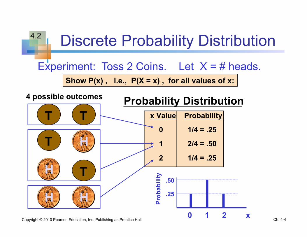
Discrete Probability Distribution

x Value Probability

0 1/4 = .25

1 2/4 = .50

2 1/4 = .25

Experiment: Toss 2 Coins. Let X = # heads.

T

T 4 possible outcomes

T

T

H

H

H H

Probability Distribution

0 1 2 x

.50

.25

Prob

abili

ty

Show P(x) , i.e., P(X = x) , for all values of x:


4.2

Probability Distribution Required Properties

∑ =x

1P(x)

§  P(x) ≥ 0 for any value of x

§  The individual probabilities sum to 1;

(The notation indicates summation over all possible x values)


4.3

Cumulative Probability Function

n  The cumulative probability function, denoted F(x0), shows the probability that X is less than or equal to x0

n  In other words,

)xP(X)F(x 00 ≤=

∑≤

=0xx

0 P(x))F(x


Expected Value

n  Expected Value (or mean) of a discrete distribution (Weighted Average)

n  Example: Toss 2 coins, x = # of heads, compute expected value of X:

E(X) = (0 x .25) + (1 x .50) + (2 x .25) = 1.0

x P(x)

0 .25

1 .50

2 .25

∑==x

P(x)x E(X) µ


Variance and Standard Deviation

n  Variance of a discrete random variable X

n  Standard Deviation of a discrete random variable X

∑ −=−=x

222 P(x)µ)(xµ)E(Xσ

∑ −==x

22 P(x)µ)(xσσ


Standard Deviation Example

n  Example: Toss 2 coins, X = # heads, compute standard deviation (recall E(x) = 1)

∑ −=x

2P(x)µ)(xσ

.707.50(.25)1)(2(.50)1)(1(.25)1)(0σ 222 ==−+−+−=

Possible number of heads = 0, 1, or 2


Functions of Random Variables

n  If P(x) is the probability function of a discrete random variable X , and g(X) is some function of X , then the expected value of function g is

∑=xg(x)P(x)E[g(X)]


Linear Functions of Random Variables

n  Let a and b be any constants.

n  a)

i.e., if a random variable always takes the value a, it will have mean a and variance 0

n  b)

i.e., the expected value of b·X is b·E(X)

0Var(a)andaE(a) ==

E(bX) = bE(X) and Var(bX) = b2Var(X)


Linear Functions of Random Variables

n  Let random variable X have mean µx and variance σ2x

n  Let a and b be any constants. n  Let Y = a + bX n  Then the mean and variance of Y are

n  so that the standard deviation of Y is

E(Y) = E(a + bX) = a + bE(X)

Var(Y ) = Var(a + bX) = b2Var(X)

XY σbσ =

(continued)


Probability Distributions

Continuous Probability Distributions

Binomial

Probability Distributions

Discrete Probability Distributions

Uniform

Normal

Ch. 4 Ch. 5


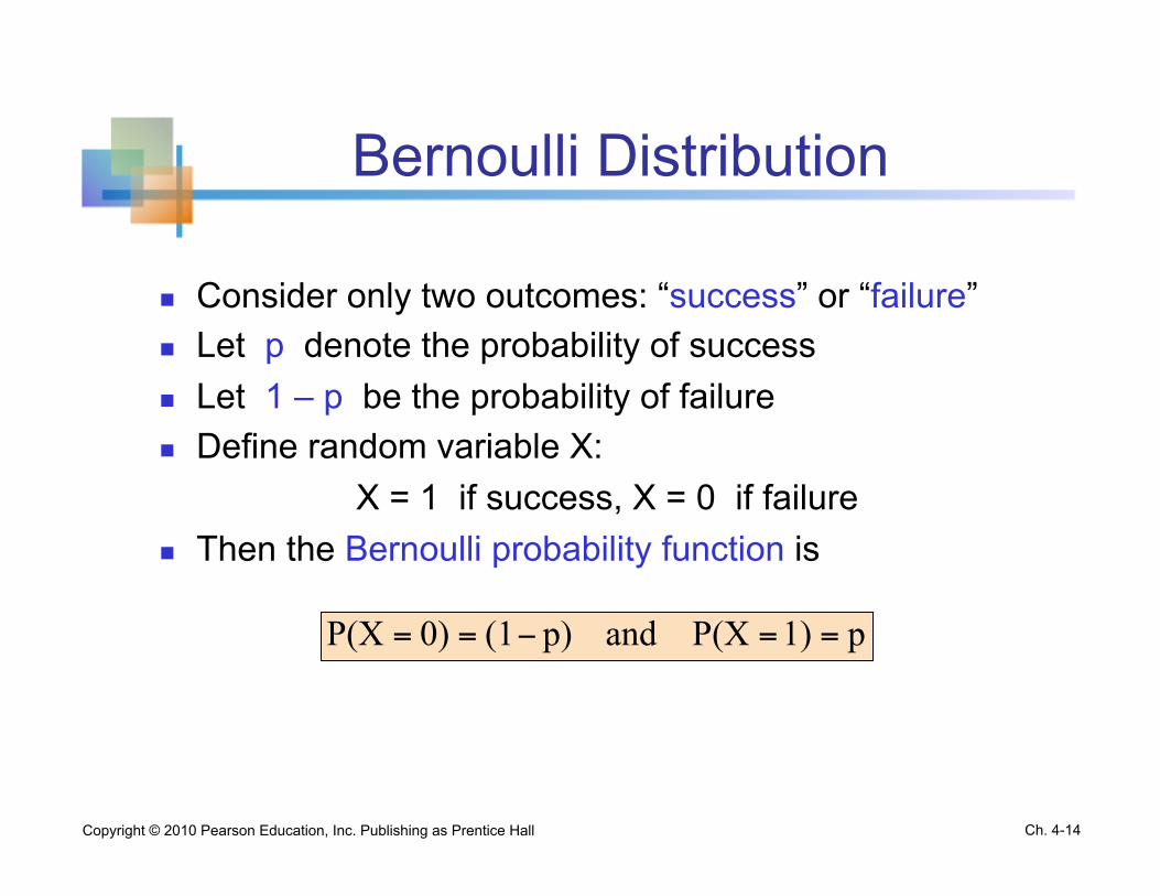
Bernoulli Distribution

n  Consider only two outcomes: “success” or “failure” n  Let p denote the probability of success n  Let 1 – p be the probability of failure n  Define random variable X:

X = 1 if success, X = 0 if failure n  Then the Bernoulli probability function is

p1)P(X andp)(10)P(X ==−==


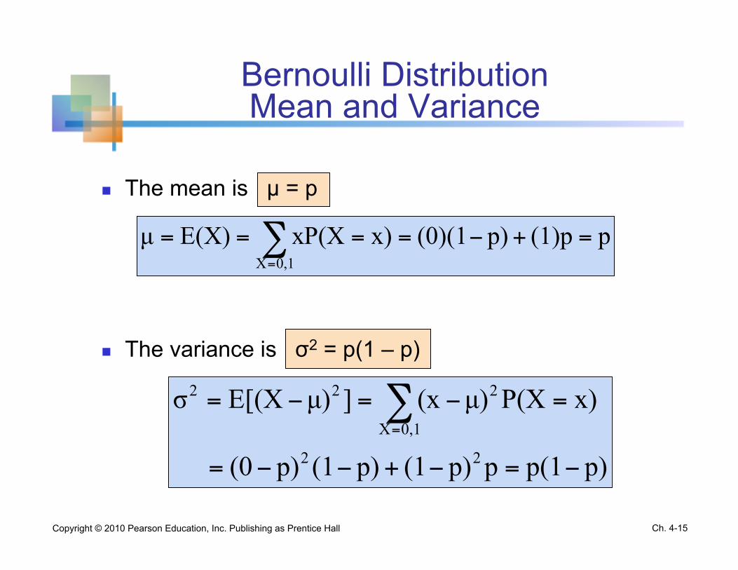
Bernoulli Distribution Mean and Variance

n  The mean is µ = p

n  The variance is σ2 = p(1 – p)

p(1)pp)(0)(1x)P(XxE(X)µ0,1X

=+−==== ∑=

p)p(1pp)(1p)(1p)(0

x)P(Xµ)(x]µ)E[(Xσ

22

0,1X

222

−=−+−−=

=−=−= ∑=


Sequences of x Successes in n Trials

n  The number of sequences with x successes in n independent trials is:

Where n! = n·(n – 1)·(n – 2)· . . . ·1 and 0! = 1

n  These sequences are mutually exclusive, since no two can occur at the same time

x)!(nx!n!Cnx −

=


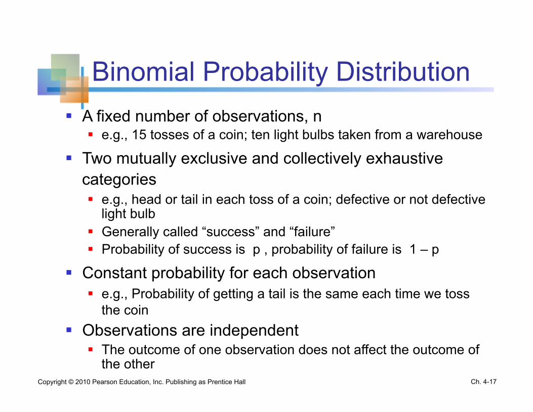
Binomial Probability Distribution §  A fixed number of observations, n

§  e.g., 15 tosses of a coin; ten light bulbs taken from a warehouse

§  Two mutually exclusive and collectively exhaustive categories §  e.g., head or tail in each toss of a coin; defective or not defective

light bulb §  Generally called “success” and “failure” §  Probability of success is p , probability of failure is 1 – p

§  Constant probability for each observation §  e.g., Probability of getting a tail is the same each time we toss

the coin §  Observations are independent

§  The outcome of one observation does not affect the outcome of the other


Possible Binomial Distribution Settings

n  A manufacturing plant labels items as either defective or acceptable

n  A firm bidding for contracts will either get a contract or not

n  A marketing research firm receives survey responses of “yes I will buy” or “no I will not”

n  New job applicants either accept the offer or reject it


Binomial Distribution Formula

P(x) = probability of x successes in n trials, with probability of success p on each trial

x = number of ‘successes’ in sample, (x = 0, 1, 2, ..., n)

n = sample size (number of trials or observations)

p = probability of “success”

P(X=x) n

x ! n x p (1- p) X n X !

( ) ! =

-

-

Example: Flip a coin four times, let x = # heads:

n = 4

p = 0.5

1 - p = (1 - 0.5) = 0.5

x = 0, 1, 2, 3, 4


Example: Calculating a Binomial Probability

What is the probability of one success in five observations if the probability of success is 0.1?

X = 1, n = 5, and p = 0.1

.32805.9)(5)(0.1)(0

0.1)(1(0.1)1)!(51!

5!

p)(1px)!(nx!

n!1)P(X

4

151

XnX

=

=

−−

=

−−

==

−

−


Binomial Distribution

n  The shape of the binomial distribution depends on the values of P and n

n = 5 P = 0.1

n = 5 P = 0.5

Mean

0 .2 .4 .6

0 1 2 3 4 5 x

P(x)

.2

.4

.6

0 1 2 3 4 5 x

P(x)

0

§  Here, n = 5 and P = 0.1

§  Here, n = 5 and P = 0.5


Binomial Distribution Mean and Variance

n  Mean

§  Variance and Standard Deviation

npE(X)µ ==

p)-np(1σ2 =

p)-np(1σ =Where n = sample size

p = probability of success (1 – p) = probability of failure


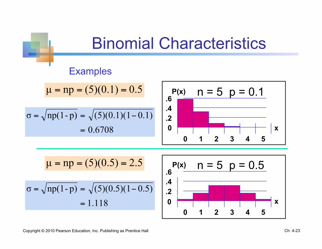
Binomial Characteristics

n = 5 p = 0.1

n = 5 p = 0.5

Mean

0 .2 .4 .6

0 1 2 3 4 5 x

P(x)

.2

.4

.6

0 1 2 3 4 5 x

P(x)

0

0.5(5)(0.1)npµ ===

0.67080.1)(5)(0.1)(1p)-np(1σ

=

−==

2.5(5)(0.5)npµ ===

1.1180.5)(5)(0.5)(1p)-np(1σ

=

−==

Examples


Using Binomial Tables

N x … p=.20 p=.25 p=.30 p=.35 p=.40 p=.45 p=.50

10 0 1 2 3 4 5 6 7 8 9

10

… … … … … … … … … … …

0.1074 0.2684 0.3020 0.2013 0.0881 0.0264 0.0055 0.0008 0.0001 0.0000 0.0000

0.0563 0.1877 0.2816 0.2503 0.1460 0.0584 0.0162 0.0031 0.0004 0.0000 0.0000

0.0282 0.1211 0.2335 0.2668 0.2001 0.1029 0.0368 0.0090 0.0014 0.0001 0.0000

0.0135 0.0725 0.1757 0.2522 0.2377 0.1536 0.0689 0.0212 0.0043 0.0005 0.0000

0.0060 0.0403 0.1209 0.2150 0.2508 0.2007 0.1115 0.0425 0.0106 0.0016 0.0001

0.0025 0.0207 0.0763 0.1665 0.2384 0.2340 0.1596 0.0746 0.0229 0.0042 0.0003

0.0010 0.0098 0.0439 0.1172 0.2051 0.2461 0.2051 0.1172 0.0439 0.0098 0.0010

Examples: n = 10, X = 3, p = 0.35: P(X = 3|n =10, p = 0.35) = .2522

n = 10, X = 8, p = 0.45: P(X = 8|n =10, p = 0.45) = .0229


Joint Probability Functions

n  A joint probability function is used to express the probability that X takes the specific value x and simultaneously Y takes the value y, as a function of x and y

n  The marginal probabilities are

y)YxP(Xy)P(x, =∩==

∑=y

y)P(x,P(x) ∑=x

y)P(x,P(y)


4.7

Conditional Probability Functions

n  The conditional probability function of the random variable Y expresses the probability that Y takes the value y when the value x is specified for X.

n  Similarly, the conditional probability function of X, given Y = y is:

P(x)y)P(x,x)|P(y =

P(y)y)P(x,y)|P(x =


Independence

n  The jointly distributed random variables X and Y are said to be independent if and only if their joint probability function is the product of their marginal probability functions:

for all possible pairs of values x and y

n  A set of k random variables are independent if and only

if

P(x)P(y)y)P(x, =

)P(x))P(xP(x)x,,x,P(x k21k21 !! =


Covariance

n  Let X and Y be discrete random variables with means µX and µY

n  The expected value of (X - µX)(Y - µY) is called the covariance between X and Y

n  For discrete random variables

n  An equivalent expression is

∑∑ −−=−−=x y

YXYX y))P(x,µ)(yµ(x)]µ)(YµE[(XY)Cov(X,

∑∑ −=−=x y

YXYX µµy)xyP(x,µµE(XY)Y)Cov(X,


Covariance and Independence

n  The covariance measures the strength of the linear relationship between two variables

n  If two random variables are statistically independent, the covariance between them is 0 n  The converse is not necessarily true


Correlation

n  The correlation between X and Y is:

n  ρ = 0 : no linear relationship between X and Y n  ρ > 0 : positive linear relationship between X and Y

n  when X is high (low) then Y is likely to be high (low) n  ρ = +1 : perfect positive linear dependency

n  ρ < 0 : negative linear relationship between X and Y n  when X is high (low) then Y is likely to be low (high) n  ρ = -1 : perfect negative linear dependency

YXσσY)Cov(X,Y)Corr(X,ρ ==


Portfolio Analysis

n  Let random variable X be the share price for stock A n  Let random variable Y be the share price for stock B

n  The market value, W, for the portfolio is given by the linear function

n  ``a’’ and ``b’’ are the numbers of shares of stock A and B,

respectively.

n  The return from holding the portfolio W:

bYaXW +=


YbXaW Δ+Δ=Δ

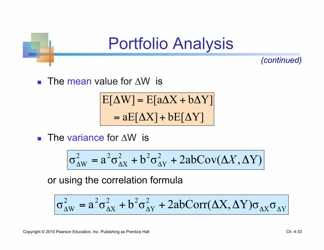
Portfolio Analysis

n  The mean value for ∆W is

n  The variance for ∆W is

or using the correlation formula

(continued)

Y]bE[X]aE[Y]bXE[aW]E[

Δ+Δ=

Δ+Δ=Δ

Y),2abCov(σbσaσ 2Y

22X

22W ΔΔ++= ΔΔΔ X

YX2Y

22X

22W σY)σX,2abCorr(σbσaσ ΔΔΔΔΔ ΔΔ++=


Example: Investment Returns

Return per $100 for two types of investments

P(∆X,∆Y) Economic condition Bond Fund X Aggressive Fund Y

0.2 Recession + $ 7 - $20

0.5 Stable Economy + 4 + 6

0.3 Expanding Economy + 2 + 35

Investment

E(∆X) = (7)(.2) +(4)(.5) + (2)(.3) = 4

E(∆Y) = (-20)(.2) +(6)(.5) + (35)(.3) = 9.5


Computing the Standard Deviation for Investment Returns


0.2 Recession + $ 7 - $20



Investment

731.(0.3)4)(2(0.5)4)(4(0.2)4)(7X)Var( 222

X

=

−+−+−=Δ=Δσ

19.37(0.3)9.5)(35(0.5)9.5)(6(0.2)9.5)(-20Y)Var( 222

Y

=

−+−+−=Δ=Δσ


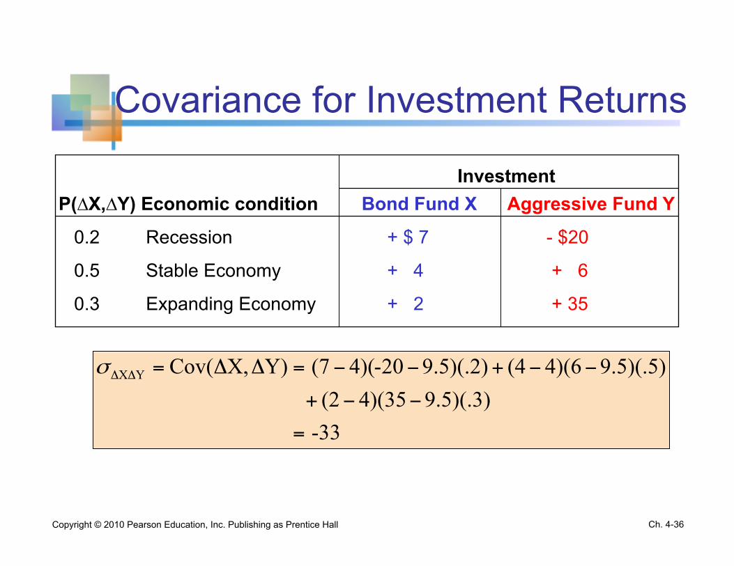
Covariance for Investment Returns


0.2 Recession + $ 7 - $20



Investment

-339.5)(.3)4)(35(2

9.5)(.5)4)(6(49.5)(.2)20-4)((7Y)X,Cov(YX

=

−−+

−−+−−=ΔΔ=ΔΔσ


Portfolio Example

Investment X: E(∆X)= 4 σ∆X = 1.73 Investment Y: E(∆Y)= 9.5 σ∆Y = 19.32 σ∆X∆Y = -33

Suppose 40% of the portfolio (W) is in Investment X

and 60% is in Investment Y: The portfolio return and portfolio variability are between the values

for investments X and Y considered individually

3.7)5.9()6(.)4(4.W)E( =+=Δ

91.10

-33)2(.4)(.6)((19.32))6(.(1.73)(.4)W)Var( 2222

=

++=Δ


Interpreting the Results for Investment Returns

n  The aggressive fund has a higher expected return, but much more risk

E(∆Y)= 9.5 > E(∆X) = 4 but σ∆Y = 19.32 > σ∆X = 1.73

n  The Covariance of -33 indicates that the two investments are negatively related and will vary in the opposite direction


Statistics for Business and Economics - Faculty and...

Documents

Transcript of Statistics for Business and Economics - Faculty and...