Statistics assignment and homework help service
12
Statistics Assignment and Homework Help Service Tutorhelpdesk David Luke Contact Us: Phone: (617) 807 0926 Web: www.tutorhelpdesk.com Email: - [email protected] Facebook: https://www.facebook.com/Tutorhelpdesk Twitter: http://twitter.com/tutorhelpdesk Blog: http://tutorhelpdesk.blogspot.com/ Tutorhelpdesk Copyright © 2010-2015 Tutorhelpdesk.com
-
Upload
tutor-help-desk -
Category
Education
-
view
27 -
download
0
Transcript of Statistics assignment and homework help service

Statistics Assignment and Homework Help Service
Tutorhelpdesk
David Luke
Contact Us:
Phone: (617) 807 0926
Web: www.tutorhelpdesk.com
Email: - [email protected]
Facebook: https://www.facebook.com/Tutorhelpdesk
Twitter: http://twitter.com/tutorhelpdesk
Blog: http://tutorhelpdesk.blogspot.com/
Tutorhelpdesk
Copyright © 2010-2015 Tutorhelpdesk.com

Tutorhelpdesk
Copyright © 2010-2015 Tutorhelpdesk.com
About Statistics: Complexity of statistics subject is well
known. Statistics involves solving complex problems having
multi-dimensional data using computational methods.
Information technology has played a vital role in handling and
simplifying such complex methods and scenarios but students
face a lot of difficulties in understanding the right application
of statistical concepts and implementing them using statistical
softwares. Our Statistics Assignment and Homework help
service has been strategized and simplified to help students in
learning statistics problem solving. We use latest and genuine
tools & softwares to make statistics easy. We deliver step by step help with statistics
assignments which is self-explanatory to make students understand the method of solving
problems without any inconvenience.
Sample Statistics Assignment and Homework Help Service Questions:
Depreciation Sample Questions
Question-1: Find the trend line equation and obtain the trend values for the following data
using the method of the least square. Also, forecast the earning for 2006.
Year :
Earning in ’000 $
1997
38
1998
40
1999
65
2000
72
2001
69
2002
60
2003
87
2004
95
Solution. Here, the number of items being 8 (i.e. even), the time deviation X will be taken
as 𝒕−𝒎𝒊𝒅 𝒑𝒐𝒊𝒏𝒕 𝒐𝒇 𝒕𝒊𝒎𝒆𝟏
𝟐 𝒐𝒇 𝒕𝒊𝒎𝒆 𝒊𝒏𝒕𝒆𝒓𝒗𝒂𝒍
to avoide the decimal numbers. Thus, the working will run as under:
Tutorhelpdesk
Copyright © 2010-2015 Tutorhelpdesk.com
Tutorhelpdesk
Copyright © 2010-2015 Tutorhelpdesk.com
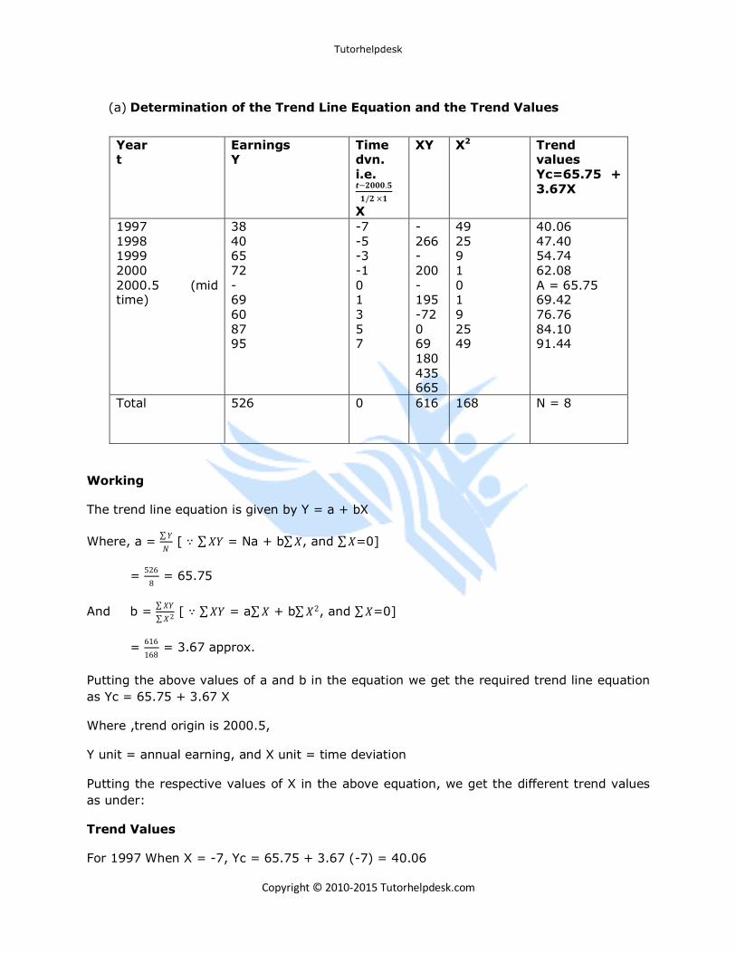
(a) Determination of the Trend Line Equation and the Trend Values
Working
The trend line equation is given by Y = a + bX
Where, a = 𝑌
𝑁 [ ∵ 𝑋𝑌 = Na + b 𝑋, and 𝑋=0]
= 526
8 = 65.75
And b = 𝑋𝑌
𝑋2 [ ∵ 𝑋𝑌 = a 𝑋 + b 𝑋2, and 𝑋=0]
= 616
168 = 3.67 approx.
Putting the above values of a and b in the equation we get the required trend line equation
as Yc = 65.75 + 3.67 X
Where ,trend origin is 2000.5,
Y unit = annual earning, and X unit = time deviation
Putting the respective values of X in the above equation, we get the different trend values
as under:
Trend Values
For 1997 When X = -7, Yc = 65.75 + 3.67 (-7) = 40.06
Year t
Earnings Y
Time dvn. i.e. 𝒕−𝟐𝟎𝟎𝟎.𝟓
𝟏/𝟐 ×𝟏
X
XY X2 Trend values Yc=65.75 + 3.67X
1997 1998 1999 2000 2000.5 (mid time)
38 40 65 72 - 69 60 87 95
-7 -5 -3 -1 0 1 3 5 7
-266 -200 -195 -72 0 69
180 435 665
49 25 9 1 0 1 9 25 49
40.06 47.40 54.74 62.08 A = 65.75 69.42 76.76 84.10 91.44
Total 526 0 616 168 N = 8
Tutorhelpdesk
Copyright © 2010-2015 Tutorhelpdesk.com
1998 When X = -5, Yc = 65.75 + 3.67 (-5) = 47.40
1999 When X =-3, Yc = 65.75 + 3.67 (-3) = 54.74
2000 When X = -1, Yc = 65.75 + 3.67 (-1) = 62.08
2001 When X =1, Yc = 65.75 + 3.67 (1) = 69.42
2002 When X = 3, Yc = 65.75 + 3.67 (3) = 76.76
2003 When X = 5, Yc = 65.75 + 3.67 (5) = 84.10
2004 When X = 7, Yc = 65.75 + 3.67 (7) = 91.44
(b) Forecasting of earnings for 2006
For 2006, X = 𝒕−𝒎𝒊𝒅 𝒑𝒐𝒊𝒏𝒕 𝒐𝒇 𝒕𝒊𝒎𝒆𝟏
𝟐 𝒐𝒇 𝒕𝒊𝒎𝒆 𝒊𝒏𝒕𝒆𝒓𝒗𝒂𝒍
= 2006−2000 .5
1
2×1
= 11
Thus, Yc = 65.75 + 3.67 (11) = 106.12
Hence, the earnings for 2005 is expected to be
= $ 106.12 × 100 = $ 106120
Tutorhelpdesk
Copyright © 2010-2015 Tutorhelpdesk.com
Question-2: Obtain the straight line trend equation for the following data by the method of
the least square.
Year : Sales in ’000
$
1995 140
1997 144
1998 160
1999 152
2000 168
2001 176
2004 180
Also, estimate the sales for 2002
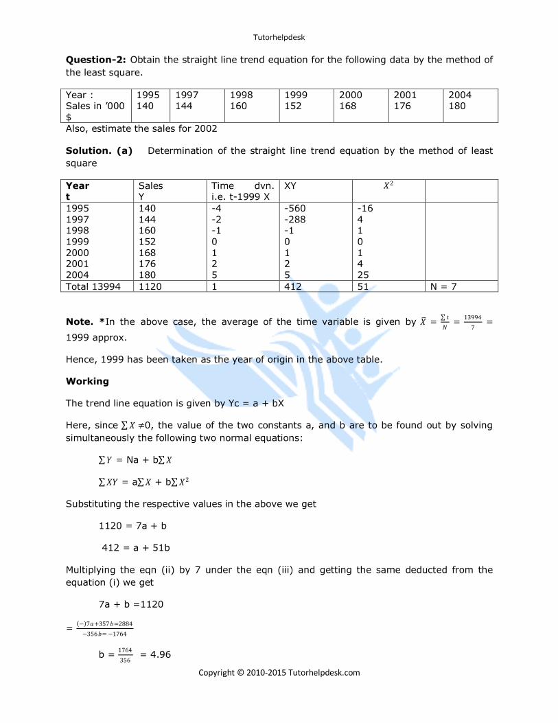
Solution. (a) Determination of the straight line trend equation by the method of least
square
Year t
Sales Y
Time dvn. i.e. t-1999 X
XY 𝑋2
1995 1997 1998 1999 2000 2001
2004
140 144 160 152 168 176
180
-4 -2 -1 0 1 2
5
-560 -288 -1 0 1 2
5
-16 4 1 0 1 4
25
Total 13994 1120 1 412 51 N = 7
Note. *In the above case, the average of the time variable is given by 𝑋 = 𝑡
𝑁 =
13994
7 =
1999 approx.
Hence, 1999 has been taken as the year of origin in the above table.
Working
The trend line equation is given by Yc = a + bX
Here, since 𝑋 ≠0, the value of the two constants a, and b are to be found out by solving
simultaneously the following two normal equations:
𝑌 = Na + b 𝑋
𝑋𝑌 = a 𝑋 + b 𝑋2
Substituting the respective values in the above we get
1120 = 7a + b
412 = a + 51b
Multiplying the eqn (ii) by 7 under the eqn (iii) and getting the same deducted from the
equation (i) we get
7a + b =1120
= − 7𝑎+357𝑏=2884
−356𝑏= −1764
b = 1764
356 = 4.96
Tutorhelpdesk
Copyright © 2010-2015 Tutorhelpdesk.com
Putting the above value of b in the equation (i) we get,
7a + 4.96 = 1120
7a = 1120 – 4.96 = 1115.04
or a = 1115.04/7 = 159.29
Putting the above values of a and b in the format of the equation we get the straight line for
trend as under:
Yc = 159.29 + 4.96X
Where, the year of working origin = 1999,
Y unit = annual sales (in ’000 $) and
X unit = time deviations.
(b)Estimation of the Sale for 2002
For 2002, X = 2002 – 1999 =3
Thus when, X = 3, Yc = 159.29 + 4.96 (3)= 159.29 + 14.88 = 174.17
Hence, the sales for 2002 are expected to be 174.17 × 103 = $ 174170.
Tutorhelpdesk
Copyright © 2010-2015 Tutorhelpdesk.com
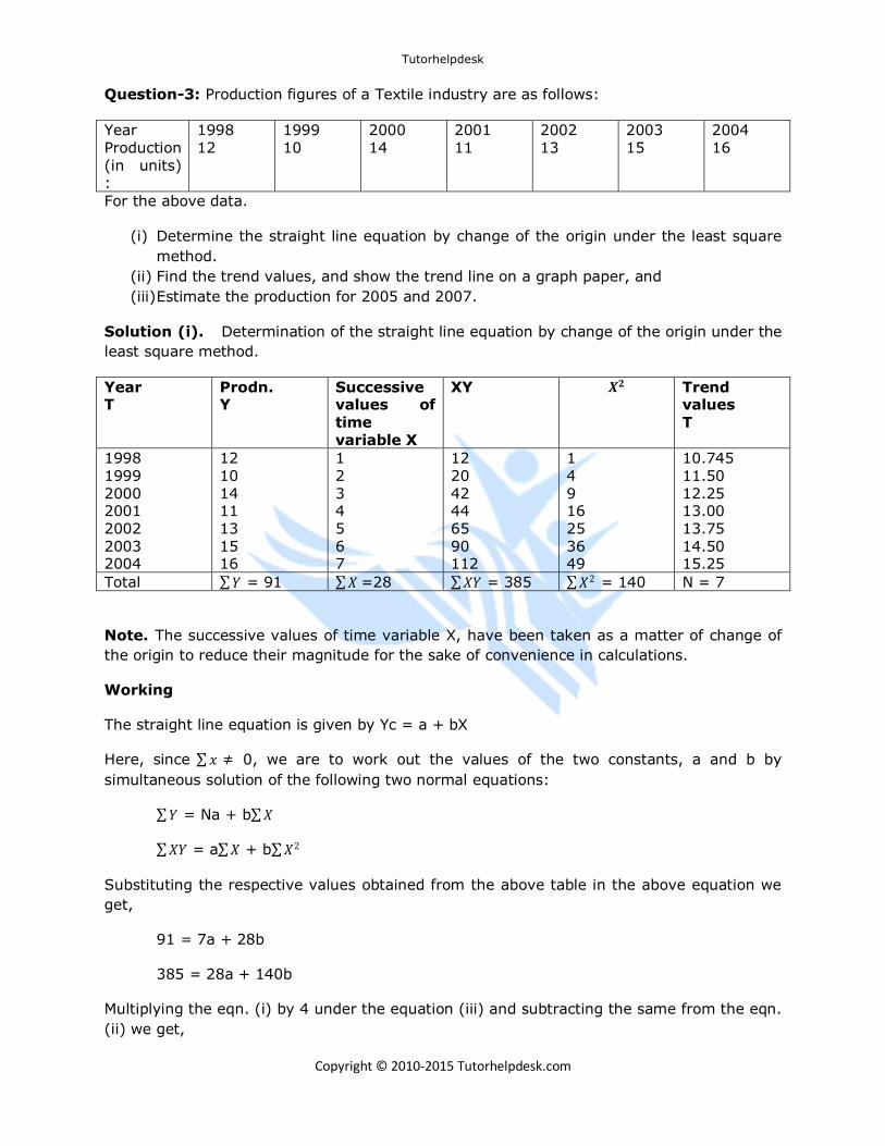
Question-3: Production figures of a Textile industry are as follows:
Year Production (in units) :
1998 12
1999 10
2000 14
2001 11
2002 13
2003 15
2004 16
For the above data.
(i) Determine the straight line equation by change of the origin under the least square
method.
(ii) Find the trend values, and show the trend line on a graph paper, and
(iii) Estimate the production for 2005 and 2007.
Solution (i). Determination of the straight line equation by change of the origin under the
least square method.
Year T
Prodn. Y
Successive values of
time variable X
XY 𝑿𝟐 Trend values
T
1998 1999 2000 2001 2002
2003 2004
12 10 14 11 13
15 16
1 2 3 4 5
6 7
12 20 42 44 65
90 112
1 4 9 16 25
36 49
10.745 11.50 12.25 13.00 13.75
14.50 15.25
Total 𝑌 = 91 𝑋 =28 𝑋𝑌 = 385 𝑋2 = 140 N = 7
Note. The successive values of time variable X, have been taken as a matter of change of
the origin to reduce their magnitude for the sake of convenience in calculations.
Working
The straight line equation is given by Yc = a + bX
Here, since 𝑥 ≠ 0, we are to work out the values of the two constants, a and b by
simultaneous solution of the following two normal equations:
𝑌 = Na + b 𝑋
𝑋𝑌 = a 𝑋 + b 𝑋2
Substituting the respective values obtained from the above table in the above equation we
get,
91 = 7a + 28b
385 = 28a + 140b
Multiplying the eqn. (i) by 4 under the equation (iii) and subtracting the same from the eqn.
(ii) we get,
Tutorhelpdesk
Copyright © 2010-2015 Tutorhelpdesk.com
28a + 140b = 385
= − 28𝑎+112𝑏=364
28𝑏=21
∴ b = 21
28 = .75
Putting the above value of b in the eqn. (i) we get,
7a + 28 (.75) = 91
= 7a = 91 – 21 = 70
∴ a = 70/7 = 10
Putting the above values of a and b in the relevant equation we get the straight line
equation naturalized as under:
Yc = 10 + 0.75 X
Where, X, represents successive values of the time variable, Y, the annual production and
the year of origin is 1997 the previous most year.
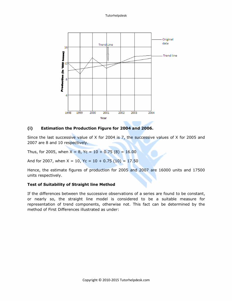
(ii) Calculation of the Trend values & Their Graphic Representation
1998 When X = 1, Yc = 10 + 0.75 (1) = 10.75
1999 When X =2, Yc = 10 + 0.75 (2) = 11.50
2000 When X = 3, Yc = 10 + 0.75 (3) = 12.25
2001 When X =4, Yc = 10 + 0.75 (4) = 13.00
2002 When X = 5, Yc = 10 + 0.75 (5) = 13.75
2003 When X = 6, Yc = 10 + 0.75 (6) = 14.50
2004 When X = 7, Yc = 10 + 0.75 (7)= 15.25
Graphic Representation of the Trend Line & the Original Data
Tutorhelpdesk
Copyright © 2010-2015 Tutorhelpdesk.com
(i) Estimation the Production Figure for 2004 and 2006.
Since the last successive value of X for 2004 is 7, the successive values of X for 2005 and
2007 are 8 and 10 respectively.
Thus, for 2005, when X = 8, Yc = 10 + 0.75 (8) = 16.00
And for 2007, when X = 10, Yc = 10 + 0.75 (10) = 17.50
Hence, the estimate figures of production for 2005 and 2007 are 16000 units and 17500
units respectively.
Test of Suitability of Straight line Method
If the differences between the successive observations of a series are found to be constant,
or nearly so, the straight line model is considered to be a suitable measure for
representation of trend components, otherwise not. This fact can be determined by the
method of First Differences illustrated as under:
Tutorhelpdesk
Copyright © 2010-2015 Tutorhelpdesk.com
Question-4. State by using the method of First Differences, if the straight line model is
suitable for finding the trend values of the following time series:
Year : Sales :
1997 30
1998 50
1999 72
2000 90
2001 107
2002 129
2003 147
2004 170
Solution. Determination of Suitability of the Straight line model by the method of
First Differences
Year T
Sales Y
First Differences
1997 1998 1999 2000 2001 2002 2003 2004
30 50 72 90 107 129 147 170
50-30 = 20 72 – 50 = 22 90 – 72 = 18 107 – 90 = 17 129 – 107 = 22 147 – 129 = 18 170 – 147 = 23
From the above table, it must be seen that the first differences in the successive
observations are almost constant by 20 or nearly so. Hence, the straight line model is quite
suitable for representing the trend components of the given series.
Tutorhelpdesk
Copyright © 2010-2015 Tutorhelpdesk.com
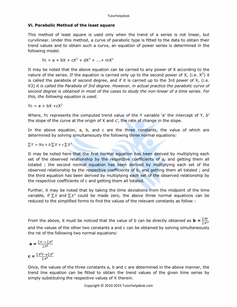
Vi. Parabolic Method of the least square
This method of least square is used only when the trend of a series is not linear, but
curvilinear. Under this method, a curve of parabolic type is fitted to the data to obtain their
trend values and to obtain such a curve, an equation of power series is determined in the
following model.
Yc = a + bX + cX2 + dX3 + ….+ mXn
It may be noted that the above equation can be carried to any power of X according to the
nature of the series. If the equation is carried only up to the second power of X, (i.e. X2) it
is called the parabola of second degree, and if it is carried up to the 3rd power of X, (i.e.
X3) it is called the Parabola of 3rd degree. However, in actual practice the parabolic curve of
second degree is obtained in most of the cases to study the non-linear of a time series. For
this, the following equation is used.
Yc = a + bX +cX2
Where, Yc represents the computed trend value of the Y variable ‘a’ the intercept of Y, b’
the slope of the curve at the origin of X and c’, the rate of change in the slope.
In the above equation, a, b, and c are the three constants, the value of which are
determined by solving simultaneously the following three normal equations:
𝑌 = 𝑁𝑎 + 𝑏 𝑋 + 𝑐 𝑋3
It may be noted here that the first normal equation has been derived by multiplying each
set of the observed relationship by the respective coefficients of a, and getting them all
totaled ; the second normal equation has been derived by multiplying each set of the
observed relationship by the respective coefficients of b, and getting them all totaled ; and
the third equation has been derived by multiplying each set of the observed relationship by
the respective coefficients of c and getting them all totaled.
Further, it may be noted that by taking the time deviations from the midpoint of the time
variable, if 𝑋 and 𝑋3 could be made zero, the above three normal equations can be
reduced to the simplified forms to find the values of the relevant constants as follow :
From the above, it must be noticed that the value of b can be directly obtained as b = 𝑿𝒀
𝑿𝟐,
and the values of the other two constants a and c can be obtained by solving simultaneously
the rst of the following two normal equations:
a = 𝒀− 𝒄 𝑿𝟐
𝑿𝟒
c = 𝑿𝟐𝒀−𝒂 𝑿𝟐
𝑿𝟒
Once, the values of the three constants a, b and c are determined in the above manner, the
trend line equation can be fitted to obtain the trend values of the given time series by
simply substituting the respective values of X therein.

Tutorhelpdesk
Copyright © 2010-2015 Tutorhelpdesk.com