1

Statistical Timing Analysis Under SpatialCorrelations

Hongliang Chang and Sachin S. Sapatnekar,Fellow, IEEE

Abstract— Process variations are of increasing concern intoday’s technologies, and can significantly affect circuitper-formance. We present an efficient statistical timing analysisalgorithm that predicts the probability distribution of th e circuitdelay considering both inter-die and intra-die variations, whileaccounting for the effects of spatial correlations of intra-dieparameter variations. The procedure uses a first-order Taylorseries expansion to approximate the gate and interconnect delays.Next, principal component analysis techniques are employed totransform the set of correlated parameters into an uncorrelatedset. The statistical timing computation is then easily performedwith a PERT-like circuit graph traversal. The run-time of ou ralgorithm is linear in the number of gates and interconnects, aswell as the number of varying parameters and grid partitionsthat are used to model spatial correlations. The accuracy ofthemethod is verified with Monte Carlo simulation. On average, for100nm technology, the errors of mean and standard deviationvalues computed by the proposed method are1:06% and�4:34%respectively, and the errors of predicting the 99% and 1%confidence point are �2:46% and �0:99% respectively . Atestcase with about 17,800 gates was solved in about500 seconds,with high accuracy as compared to a Monte Carlo simulation thatrequired more than 15 hours.

Index Terms— Circuit, Deep submicron, Timing analysis,VLSI

I. I NTRODUCTION

PROCESS variations have become an increasing concern inintegrated circuits as circuit sizes continue to increase and

feature sizes continue to shrink. As device and interconnectparameters such as physical dimensions show variability, theprediction of circuit performance is becoming a challengingtask. Conventional static timing analysis (STA) handles theproblem of variability by analyzing a circuit at multipleprocess corners. However, it is generally accepted that such anapproach is inadequate, since the complexity of the variationsin the performance space implies that if a small number ofprocess corners is to be chosen, these corners must be veryconservative and pessimistic. For true accuracy, this can beovercome by using a larger number of process corners, but thenthe number of corners that must be considered for an accuratemodeling will be too large for computational efficiency.

The limitations of traditional STA techniques lie in theirdeterministic nature. An alternative approach that overcomesthese problems is statistical STA, which treats delays not asfixed numbers, but as probability density functions (PDF’s),

This work was supported in part by the NSF under award CCR-0205227and by the SRC under contract 2003-TJ-1092.

Hongliang Chang is with Department of Computer Science and Engineeringand Sachin S. Sapatnekar is with Department of Electrical and ComputerEngineering, both in the University of Minnesota.

taking the statistical distribution of parametric variations intoconsideration while analyzing the circuit.

Process variations can be classified into the following cate-gories:inter-die variationsare the variations from die to die,while intra-die variationscorrespond to variability within asingle chip. Inter-die variations affect all the devices onsamechip in the same way, e.g., making the transistor gate lengthsof devices on the same chip all larger or all smaller, whilethe intra-die variations may affect different devices differentlyon the same chip, e.g., making some devices have smallertransistor gate lengths and others larger transistor gate lengths.

It used to be the case that the inter-die variations dominatedintra-die variations, so that the latter could be safely neglected.However, in modern technologies, intra-die variations arerapidly and steadily growing and can significantly affect thevariability of performance parameters on a chip [1]. Theincrease in intra-chip parameter variations is due to the effectssuch as micro-loading in the etch, variation in photoresistthickness, optical proximity effects and stepper within-fieldaberrations as the manufacturing sizes approach the opticalresolution limit [2]. Intra-die variation is spatially correlated:it is locally layout-dependent and circuit-specific, i.e.,deviceswith similar layout patterns and proximity structures tendtohave similar characteristics; it is globally location-dependent,i.e., devices located close to each other are more likely to havethe similar characteristics than those placed far away.

Due to the increasing effect of intra-die variations, severalcommercial flows have begun to include intra-die variationsinthe last few years, e.g., the OCV (On-Chip Variation) analysisin Synopsys’s PrimeTime and the LCD (Linear Combinationof Delay) mode of IBM’s EinsTimer. In literature, a numberof studies on statistical timing analysis have focused oncircuit performance prediction considering intra-die variation.Continuous methods [3]–[6] use analytical approaches to findclosed-form expressions for the PDF of the circuit delay. Forsimplicity, these methods often assume a normal distributionfor the gate delay, but even so, finding the closed-from expres-sion of the circuit distribution is still not an easy task. Discretemethods [7]–[9] are not limited to normal distributions, andcan discretize any arbitrary delay distribution as a set of tuples,each corresponding to a discrete delay and its probability.Thediscrete probabilities are propagated through the circuitto finda discrete PDF for the circuit delay. However, this method isliable to suffer from the problem of having to propagate anexponential number of discrete point probabilities. In [10], anefficient method was proposed by modeling arrival times ascumulative density functions and delays as probability densityfunctions and by defining operations ofaddandmaxon these

2

functions. Alternatively, instead of finding the distribution ofcircuit delay directly, several attempts have been made to findupper and lower bounds for the circuit delay distribution [5],[7], [11].

Although many prior works have dealt with intra-chip varia-tions, most of them have ignored intra-chip spatial correlationsby simply assuming zero correlations among devices on thechip. The difficulty in considering spatial correlations betweenparameters is that it can result in complicated path correlationstructures that are hard to deal with. The authors of [6]consider correlation between delays among the transistorsinside a single gate (but not correlations between gates). Thework in [12] uses a Monte Carlo sampling-based frameworkto analyze circuit timing on a set of selected sensitizable truepaths. Another method in [5] computes path correlations on thebasis of pair-wise gate delay covariances and used an analyticmethod to derive lower and upper bounds of circuit delay. Thestatistical timing analyzer in [13] takes into account capacitivecoupling and intra-die process variation to estimate the worstcase delay of critical path. Two parameter space techniques,namely, the parallelepiped method and the ellipsoid method,and a performance-space procedure, the binding probabilitymethod, were proposed in [14] to find either bounds or theexact distribution of the minimum slack of a selected set ofpaths. The approach in [3] proposes a model for spatial corre-lation and a method of statistical timing analysis to computethe delay distribution of a specific critical path. However,thePDF for a critical path may not be a good predictor of thedistribution of the circuit delay (which is the maximum of allpath delays), as explained in Section II. Moreover, the methodmay be computationally expensive when the number of criticalpaths is too large. In [15], the authors further extended theirwork in [3], [7] to compute an upper bound on the distributionof exact circuit delay.

In this paper, we will propose an algorithm for statisticalSTA that computes the distribution of circuit delay while con-sidering spatial correlations. We will model the circuit delayas a correlated multivariate normal distribution, consideringboth gate and wire delay variations. In order to manipulatethe complicated correlation structure, the Principal ComponentAnalysis (PCA) technique is employed to transform the setsof correlated parameters into sets of uncorrelated ones. Thestatistical timing computation is then performed with a PERT-like circuit graph traversal. The complexity of the algorithmis O(p � n � (Ng +NI)), which is linear in the number ofgatesNg and interconnectsNI , and also linear in the numberof varying parametersp and the number of grid squaresnthat are used to model variational regions. In other words, thecost is, at worst,p� n times the cost of a deterministic STA.We believe that this is the first method that can fully handlespatially correlated distributions under reasonably general as-sumptions, with a complexity that is comparable to traditionaldeterministic STA. This work can also be extended, using thesame framework of maximum of delays (Section IV-C), to findthe distribution of minimum of delays which can be appliedto analysis such as computing minimum delay distributionsfor short-path analysis (to check for hold time violations), forrequired arrival time (RAT) analysis, etc.

The remainder of the paper is organized as follows. Sec-tion II formally formulates the problem to be solved in thiswork. Section III explains the model used for process variationand spatial correlation of intra-die variation. The algorithm ispresented in Section IV and its run time complexity analysisisgiven in the following section. The extension to handle inter-chip variation and spatially uncorrelated intra-chip componentsis introduced in Section VI. The extension to compute min-imum of delays is also presented in Section VI. Finally, alist of experimental results and their analysis are shown inSection VII.

II. PROBLEM FORMULATION

Under process variations, parameter values such as the gatelength, the gate width, the metal line width and the metal lineheight are random variables. Some of these variations suchas across-chip linewidth variations (ACLV) are deterministic,while others are random: this work will focus on the effects ofrandom variations, and will model these parameters as randomvariables. The gate and interconnect delays, as functions ofthese parameters, also become random variables. Given appro-priate modeling of process parameters or gate and interconnectdelays, the task of statistical STA is to find the PDF of thecircuit delay.

The static timing analysis works with the usual translationfrom a combinational circuit to a timing graph [16]. The nodesin this graph correspond to the circuit primary inputs/outputsand gate input/output pins. The edges are of two types: oneset corresponds to the pin-to-pin delay arcs within a gate, andthe other set to interconnections from the drivers to receivers.The edges are weighted by the pin-to-pin gate delay, andinterconnect delay, respectively. The primary inputs of thecombinational circuit are connected to a virtual source node,and the primary outputs to a virtual sink node with directedvirtual edges. In the case that primary inputs arrive at differenttimes, the virtual edges from the virtual source to the primaryinputs are assigned weights of the arrival times. Likewise,ifthe required times at the primary outputs are different, theweights of the edges from the outputs to the virtual sink areappropriately chosen.

For a combinational logic circuit, the problem of statictiming analysis is to compute the longest path delay in thecircuit from any primary input to any primary output, whichcorresponds to length of the longest path in the timing graph.In static timing analysis, the technique that is commonlyreferred to in the literature as PERT (Program Evaluation andReview Technique) is commonly used1. This procedure startsfrom the source node to traverse the graph in a topologicalorder and uses asumoperation ormaxoperation (at a multi-fanin node) to find the longest path at the sink node. Fordetails, the reader may refer to [16], [17].

Since we will employ a PERT-like traversal to analyze thedistribution of circuit delay, we define a statistical timing graphof a circuit, as in the case of deterministic STA.

1In reality, this is actually the critical path method (CPM) in operationsresearch. However, we will persist with the term “PERT,” which is widelyused in the static timing analysis literature.

3

Definition 2.1: Let Gs = (V;E) be a timing graph fora circuit with a single source node and a single sink node,whereV is a set of nodes andE a set of directed edges. ThegraphGs is called a statistical timing graph if each edgei isassigned a weightdi, wheredi is a random variable, wherethe random variables may be uncorrelated or correlated. Theweight associated with an edge corresponds to gate delay orinterconnect delay. For a virtual edge, the weight is randomvariables with mean of its deterministic value and standarddeviation of zero and it is independent from any other edges.

Definition 2.2: Let a pathpi be a set of ordered edgesfrom the source node to the sink node inGs, andDi be thepath length distribution ofpi, computed as the sum of theweightsdk for all edgesk on the path. Finding the distributionof Dmax = max(D1; : : : ; Di; : : : ; Dnpaths) among all paths(indexed from 1 tonpaths) in the graphGs is referred to asthe problem of statistical static timing analysis (SSTA) ofacircuit.

Note that for the same nominal design, the identity of thelongest path may change, depending on the random valuestaken by the process parameters. Therefore, finding the delaydistribution of one critical path at a time is not enough, andcorrelations between paths must be considered in finding themax of the PDF’s of all paths. Such an analysis is essentialfor finding the probability of failure of a circuit, which isavailable from the cumulative density function (CDF) of thecircuit delay.

For an edge-triggered sequential circuit, the statisticaltim-ing graph can be constructed similarly by breaking the circuitinto a set of combinational blocks between latches, and theanalysis includes statistical checks on setup and hold timeviolations. The former requires the computation of the dis-tribution of the maximum arrival time at the latches, whichrequires the solution of the SSTA problem as defined above.On the other hand, the latter problem needs the distributionof the minimum arrival time at the latches to be computed,and this can be solved by a trivial extension of the frameworkfor the SSTA problem proposed in the paper, using minimumoperators, as will be mentioned in Section VI-C, instead ofmaximum operators.

Our approach to solve the SSTA problem is based onthe following assumption on the distribution of the processparameter values:

Assumption 1The process parameter values are assumed to benormally distributed random variables.

The gate and interconnect delays, being functions of the fun-damental process parameters, are approximated using a first-order Taylor series expansion. We will show that as a resultof this, all edges in graphGs are normally distributed randomvariables. Since we consider spatial correlations of the processparameters, it turns out that some of the delays are correlatedrandom variables. Furthermore, the circuit delayDmax ismodeled as a multivariate normal distribution. Although theclosed form of circuit delay distribution is not normal, weshow that the loss of accuracy is not significant under thisapproximation.

III. M ODELING PARAMETER VARIATIONS

In this section, we will introduce the model used forintra-chip variations with spatial correlation. Althoughweconsider only intra-die variations of parameters at this point,the extension of this work to handle inter-die variations willbe introduced later in Section VI-A.

A. Components of Intra-Chip Variations

The intra-chip parametric variationÆintra can be decom-posed into three components, a deterministic global componentÆglobal, a deterministic local componentÆlo al and a randomcomponent� [18]Æintra = Æglobal + Ælo al + �: (1)

The global component,Æglobal, is location-dependent.Across the die or reticle field, it can be modeled by a slantedplane and expressed as a simple function of its locationÆglobal(x; y) = Æ0 + Æxx+ Æyy; (2)

where (x; y) is its die location,Æx and Æy are gradients ofparameter indicating the spatial variations of parameter alongthe x andy directions respectively.

The local component,Ælo al, is proximity-dependent andlayout-specific. The random component,�, stands for therandom intra-chip variation and the vector of all randomcomponents across the chip or reticle field has a correlatedmultivariate normal distribution due to spatial correlation ofthe intra-chip variation~� � N(0;�); (3)

where� is the covariance matrix of parameters. The detailedmodel for this covariance matrix will be described in thenext section. For spatially uncorrelated parameters,� becomesa diagonal matrix where the entries represent variances. Ifthe variances of the parameters described by this matrix areassumed to be uniform across the chip, then� is a multipleof the identity matrix.

In this paper, we will only consider the impact of global andrandom components. However, the local component can alsobe included in the model, given, for instance, the chip layoutand pre-characterized spatial maps of parameters as in [19].

Under intra-die variation, the value of parameterp locatedat (x; y) can be modeled asp = �p+ Æxx+ Æyy +N(0; �); (4)

where�p is the nominal design parameter value at die location(0; 0).In this way, all parameter variations are modeled as location-

dependent normally distributed random variables.In this work, for transistors, we consider the following

process parameters [20] as random variables: transistor lengthLg and widthWg , gate oxide thicknessTox, doping concen-tration densityNa; for interconnect, at each metal layer, weconsider the following parameters: metal widthWintl , metalthicknessTintl and ILD thicknessHILDl , where the subscriptl represents that the random variable is of layerl, wherel = 1 : : : nlayers. Among all the parameters listed above,Lg

4

b

a c

(1,1) (1,2) (1,3)

(2,1) (2,2) (2,3)

(3,1) (3,2) (3,3)

u vp q

e

(1,4)

(2,4)

(3,4)

(4,1) (4,2) (4,3) (4,4)

d

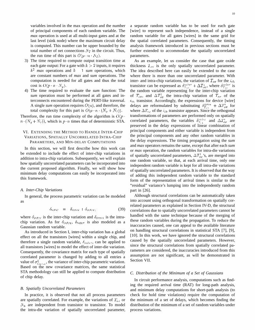
Fig. 1. Grid model for spatial correlations

is observed to exhibit largest parameter variability and alsohas the most important impact on circuit performance whenit shows variations [20]. We believe that this framework isgeneral enough that it can be applied to handle variations ofother parameters as well.

B. Spatial Correlations

To model the intra-die spatial correlations of parameters,wepartition the region of die or reticle field2 intonrow�n ol = ngrids. Since devices [wires] close to each other are morelikely to have more similar characteristics than those placedfar away, we assume perfect correlations among the devices[wires] in the same grid, high correlations among those inclose grids and low or zero correlations in far-away grids. Forexample, in Figure 1, gatesa and b (whose sizes are shownto be exaggeratedly large) are located in the same grid square,and it is assumed that their parameter variations (such as thevariations of their gate length), are always identical. Gate aand lie in neighboring grids, and their parameter variationsare not identical but highly correlated due to their spatialproximity (for example, when gatea has a larger than nominalgate length, it is highly probable that gate will have a largerthan nominal gate length, and less probable that it will haveasmaller than nominal gate length). On the other hand, gatesaandd are far away from each other, their parameters may beuncorrelated, (e.g., when gatea has a larger than nominal gatelength, the gate length ford may be either larger or smallerthan nominal).

Our algorithm makes a second assumption on the distribu-tion of process parameters:

Assumption 2It is assumed that nonzero correlations may existonly among the same type of process parameters indifferent grids, and there is no correlation betweendifferent types of process parameters3.

2The same model can be used to model the parameter variations across areticle field containing multiple chips, in which case, these multiple chips canbe analyzed simultaneously and the maximum of the delays at the POs of allchips is the distribution of chip delay. This does not changethe complexityof the algorithm, since the number of dies in a reticle field isa small integer.

3This assumption is not critical to the correctness of our procedure,but is used in our experimental results. In case the assumption is notstrictly true [21], our method is still general enough to handle correlationsbetween parameters of different types, either by decomposing the correlatedparameters into an uncorrelated set using an orthogonal transformation suchas the principal component analysis (PCA) technique, or by constructing acovariance matrix for all correlated parameters.

For example, theLg values for transistors in a grid arecorrelated with those in nearby grids, but are uncorrelatedwithother parameters such asWg or Wintl in any grid. (Note herethat we consider interconnect parameters in different layers tobe “different types of parameters,” e.g.,Wint1 andWint2 areuncorrelated.)

Under this model, the parametric variation for a spatiallycorrelated parameter in a single grid at location(x; y) can bemodeled using a single random variablep(x; y). In total, thisrepresentation requiresn random variables, each representingthe value of a parameter in one of then grids, and a covariancematrix of sizen�n representing the spatial correlations amongthe grids. The covariance matrix could be determined fromdata extracted from manufactured wafers. For example, a teststructure methodology was developed to support the evaluationof process parameter variations in [22]. The number of gridregions divided can be also determined using the test structuremethodology by refining the number of grids until delaydistribution of test structure converges or changes only withina small tolerance range. In this work, due to the lack of accessto real wafer data, we use the correlation matrix derived fromthe spatial correlation model in [3]. However, we believe thatour model is more general than the model used in [3], since itis purely based on neighborhood. For example, consider againthe case in Figure 1, by our model, the parameter in grid(1; 2)has equal correlations with that in grid(1; 1) and(1; 3). Whileby the model of [3], it will have higher correlation with grid(1; 1) than grid(1; 3), i.e., the correlations are uneven at thetwo neighbors of grid(1; 2).

For clarity of presentation, we here assume that all typesof parameters have spatial correlations. In manufacturing,due to effects such as random dopant fluctuations, the intra-chip variations of some parameters are truly uncorrelatedfrom transistor to transistor. The extension of this work toincorporate the effect of spatially uncorrelated parameters willbe shown in Section VI.

IV. STATISTICAL TIMING ANALYSIS ALGORITHM

The core statistical STA method is described in this section,and its description is organized as follows. At first, in sec-tion IV-A, we will describe how we model the distributionsof gate and interconnect delays as normal distributions, giventhe PDF’s that describe the variations of various parameters.In general, these PDF’s will be correlated with each other.In section IV-B, we will show how we can simplify thecomplicated correlated structure of parameters by orthogonaltransformations. Section IV-C will describe the PERT-liketraversal algorithm on the statistical timing graph by demon-strating the procedure for the computation ofmax and sumfunctions. Finally, Section IV-D will explain why orthogonaltransformations are important in our method.

A. Modeling Gate/Interconnect Delay PDF’s

In this section, we will show how the variations in theprocess parameters are translated into PDF’s that describethevariations in the gate and interconnect delays that correspondto the weights on edges of the statistical timing graph.

5

In section III, the geometrical parameters associated withthe gate and interconnect are modeled as normally distributedrandom variables. Before we introduce how the distributionsof gate and interconnect delays will be modeled, let us firstconsider an arbitrary functiond = F (~P ) that is assumed tobe a function on a set of parameters~P , where eachpi 2 ~Pis a random variable with a normal distribution given bypi �N(�pi ; �pi).

We can approximate the functiond linearly using a firstorder Taylor expansiond = d0 + X8 parameterspi ��F�pi �0�pi; (5)

whered0 is the nominal value ofd, calculated at the nominalvalues of parameters in~P , �F�pi is computed at the nominalvalues ofpi, �pi = pi��pi is a normally distributed randomvariable and�pi � N(0; �pi).

In this approximation,d is modeled as a normal distribution,since it is a linear combination of normally distributed randomvariables. Its mean�d, and variance�2d are�d = d0 (6)�2d = X8i ��F�pi �20 �2pi + 2X8i6=j ��F�pi �0 � �F�pj �0 ov(pi; pj);(7)

where ov(pi; pj) is the covariance ofpi andpj .It is reasonable to ask whether the approximation ofd as

a normal distribution is valid, since the distribution ofd may,strictly speaking, not be Gaussian. We can say that when�pihas relatively small variations, the first order Taylor expansionis adequate and the approximation is acceptable with littlelossof accuracy. This is generally true of intra-chip variations,where the process parameter variations are relatively smallin comparison with the nominal values. For this reason, asfunctions of process parameters, the gate and interconnectdelays can be approximated as a sum of normal distributions(which is also normal) applying equation (5).

Computing the PDF of interconnect delay:In this work, weuse the Elmore delay model for simplicity to calculate the in-terconnect delays4. Under the Elmore model, the interconnectdelay is a function of the vector of resistances,~Rw, the vectorof capacitances,~Cw, of all wire segments in the interconnecttree, and the vector of input load capacitances,~Cg , of thefanout gates, or receivers:dint = Dint(~Rw; ~Cw; ~Cg): (8)

Since the resistances and capacitances above are determined bythe process parameters~P of the interconnect and the receivers,such asWintl , Tintl , HILDl , Wg , Lg andTox, the sensitivitiesof the interconnect delay to a parameterpi can be found by

4However, it should be emphasized that any delay model may be used, andall that is needed is the sensitivity of the delay to the process parameters. Forexample, through a full circuit simulation, the sensitivities may be computedby performing adjoint sensitivity analysis.

using the chain’s rule�dint�pi = X8Rwk2~Rw �Dint�Rwk �Rwk�pi + X8Cwk2~Cw �Dint�Cwk �Cwk�pi+ X8Cgk2~Cg �Dint�Cgk �Cgk�pi : (9)

The distribution of interconnect delay can then be approxi-mated on the computed sensitivities.

We will now specifically consider the factors that affectthe interconnect delay associated with edges in the statisticaltiming graph. Recall that under our model, we divide thechip area into grids so that the parameter variations withina grid are identical, but those in different grids exhibit spatialcorrelations. Now consider an interconnect tree with severaldifferent segments that reside in different grids. The delayvariations in the tree are affected by the parameter variations ofwires in all grids that the tree traverses. For example, in Figure1, consider the two segmentsuv and pq in the interconnecttree driven by gatea. Segmentuv passes through the grid(1; 1) andpq through the grid(1; 2). Then the resistance andcapacitance of segmentuv should be calculated based on theprocess parameters of grid(1; 1), while the resistance andcapacitance of segmentpq should be based on those of grid(1; 2). Hence, the distribution of the interconnect tree delayis actually a function of random variables of interconnectparameters in both grid(1; 1) and grid (1; 2), and shouldincorporate any correlations between these random variables.Similarly, if the gates that the interconnect tree drives residein different grid locations, the interconnect delay to any sinkis also a function of random variables of gate parameters ofall grids in which the receivers are located.

In summary, the distribution of interconnect delay functioncan be approximated bydint = d0int +Xi��g h �Dint�Lig i0 �Lig +Xi��g h �Dint�Wig i0 �Wig (10)+Xi��g h �Dint�Tiox i0 �Tiox + nlayerXl=1 ( Xi��int � �Dint�Wiintl �0 �Wiintl+ Xi��int � �Dint�Tiintl �0 �Tiintl + Xi��int � �Dint�HiILDl �0 �HiILDl� ;where d0int is the interconnect delay value calculated with

nominal values of parameters,�g is the set of indices of gridsthat all the receivers reside in,�int is the set of indices ofgrids that the interconnect tree traverses, and�Lig = Lig��LigwhereLig is the random variable representing transistor lengthin the ith grid. The parameters�W ig , �T iox, �W iintl , �T iintland�H iILDl are similarly defined. As before, the subscript “0”next to each sensitivity represents the fact that it is evaluatedat the nominal point.

Computing the PDFs of gate delay and output signaltransition time: The distribution of gate delay and outputsignal transition time at the gate output can be approximatedin a similar manner as described above, given the sensitivitiesof the gate delay to the process parameters.

Consider a multiple-input gate, letdpinigate be the gate delayfrom theith input to the output andSpiniout be the corresponding

6

output signal transition time. In general, bothdpinigate andSpinioutcan be written as a function of the process parameters~P ofthe gate, the loading capacitance of the driving interconnecttree ~Cw and the succeeding gates that it drives~Cg , and theinput signal transition timeSpiniin at this input pin of the gatedpinigate = Dgate(~P ; ~Cw; ~Cg ; Spiniin ); (11)Spiniout = Sgate(~P ; ~Cw; ~Cg ; Spiniin ): (12)

The distributions ofdpinigate andSpiniin can be approximated asGaussians using linear expressions of parameters, where themean values ofdpinigate or Spiniin can be found by using themean values of~P , ~Cw, ~Cg andSpiniin in functionsDgate orSgate, and the sensitivities of eitherdpinigate or Spiniin to processparameters can be computed applying the chain’s rule. Thederivatives of ~Cw and ~Cg to the process parameters can beeasily computed, as~Cw and ~Cg are functions of processparameters. The input signal transition time,Sin, is a functionof the output transition time of the preceding gate and the delayof the interconnect connecting the preceding gates and thisgate, where both interconnect delay (as discussed earlier)andoutput transition time of the preceding gate (as will be shownin the next paragraph) are Gaussian random variables thatcan be expressed as a linear function of parameter variations.Therefore, at a gate input, the input signal transition timeSinis always given as a normally distributed random variable witha mean and first-order sensitivities to the parameter variations.

To consider the effect of non-ideal input signal on gatedelay, the output signal transition timeSout at each gate outputneeds to be computed in addition to pin-to-pin delay of thegate. In conventional static timing analysis,Sout is set toSpinioutif the path ending at the output of the gate traversing theith input pin has the longest path delaydpathi . In statisticalstatic timing analysis, each of the paths through differentgateinput pins has a certain probability to be the longest path.Therefore,Sout should be computed as a weighted sum of thedistributions ofSpiniout , where the weight equals the probabilitythat the path through theith pin is the longest among allothers:Sout = X8input pin ifProb[dpathi > max8j 6=i(dpathj )℄� Spiniout g; (13)

wheredpathi is the random path delay variable at the gate out-put through theith input pin. The result ofmax8j 6=i(dpathj )℄is a random variable representing for the distribution ofmaximum of multiple paths. As will be discussed later inSection IV-C,dpathi and max8j 6=i(dpathj ) can be approxi-mated as Gaussians usingsum and max operators, and theircorrelation can easily be computed. Therefore, finding thevalue ofProb[dpathi > max8j 6=i(dpathj ), i.e. Prob[dpathi �max8j 6=i(dpathj > 0) becomes computing the probability of aGaussian random variable greater than zero, which can easilybe found from a look-up table. As eachSpiniout is a Gaussianrandom variable in linear combination of parameter variations,Sout is therefore also a Gaussian distributed random variableand its sensitivities to all process parameters�Sout�pi can easilybe found from its linear expression of parameters.

B. Orthogonal Transformation of Correlated Variables

In statistical timing analysis without spatial correlations,correlations due to reconvergent paths has long been an

obstacle. When the spatial correlation of process parameters isalso taken into consideration, the correlation structure becomeseven more complicated. To make the problem tractable, we usethe Principal Component Analysis (PCA) technique [23] totransform the set of correlated parameters into an uncorrelatedset.

PCA is a method that can be employed to examine therelationship among a set of correlated variables. Given a setof correlated random variables~X with a covariance matrixR,PCA can transform the set~X into a set of mutually orthogonalrandom variables,~X 0, such that each member of~X 0 has zeromean and unit variance. The elements of the set~X 0 are calledprincipal components in PCA, and the size of~X 0 is no largerthan the size of~X. Any variablexi 2 ~X can then be expressedin terms of the principal components~X 0 as follows:xi = (Xj p�j � vij � x0j)�i + �i; (14)

wherex0j is a principal component in set~X 0, �j is the jtheigenvalue of the covariance matrixR, vij is the ith elementof the jth eigenvector ofR, and�i and�i are, respectively,the mean and standard deviation ofxi.

Since we assume that different types of parameters areuncorrelated, we can group the random variables of parametersby types and perform principal component analysis in eachgroup separately, i.e., we compute the principal componentsfor ~Lg , ~Wg , ~Tox, ~Na, ~Wintl and ~Tintl individually. Clearly,not only are the principal components of the same type ofparameters independent, but so are the principal componentsof different type of parameters.

For instance, let~Lg be a random vector representing tran-sistor gate length variations in all grids and it is of multivariatenormal distribution with covariance matrixRLg . Let ~L0g bethe set of principal components computed by PCA. Then anyLig 2 ~Lg representing the variation of transistor gate length ofthe ith grid can then be expressed as a linear function of theprincipal componentsLig = �Lig + ai1 � l01g + � � �+ ait � l0tg ; (15)

where�Lig is the mean ofLig, l0ig is a principal component in~L0g, all l0ig are independent with zero means and unit variances,and t is the total number of principal components in~L0g .

In this way, any random variable in~Wg, ~Tox, ~Na, ~Wintl ,~Tintl and ~HILDl can be expressed as a linear function of thecorresponding principal components in~W 0g, ~T 0ox, ~N 0a, ~W 0intl ,~T 0intl and ~H 0ILDl . Superposing the set of rotated randomvariables of parameters on the original random variables ingate or interconnect delay in equation (10), the expressionof gate or interconnect delay is then changed to the linearcombination of principal components of all parametersd = d0 + k1 � p01 + � � �+ km � p0m; (16)

wherep0i 2 ~P 0 and ~P 0 = ~L0g [ ~W 0g [ ~T 0ox [ ~N 0a [ ~W 0intl [ ~T 0intl [~H 0ILDl andm is the size of~P 0.Note that all of the principal componentsp0i that appear in

equation (16) are independent. Equation (16) has the followingproperties:

7

Property 1Since allp0i are orthogonal, the variance ofd can besimply computed as�2d = mXi=1 k2i : (17)

Property 2The covariance betweend and any principal compo-nentp0i is given by ov(d; p0i) = ki�2p0i = ki: (18)

In other words, the coefficient ofp0i is exactly thecovariance betweend andp0i.

Property 3Let di anddj be two random variables:di = d0i + ki1 � p01 + � � �+ kim � p0m; (19)dj = d0j + kj1 � p01 + � � �+ kjm � p0m: (20)

The covariance ofdi and dj , ov(di; dj), can becomputed by ov(di; dj) = mXr=1 kirkjr : (21)

In comparison, without an orthogonal transformation,the value of ov(di; dj) has to be computed by amore complicated formula as will be described insection IV-D.

C. PERT-like Traversal of Statistical STA

Using the techniques discussed up to this point, all edgesof the statistical timing graph may be modeled as normallydistributed random variables. In this section, we will describea procedure for finding the distribution of the statistical longestpath in the graph.

In conventional deterministic STA, the PERT algorithm canbe used to find the longest path in a graph by traversing it intopological order using two types of functions:� the sumfunction, and� the max function.

In our statistical timing analysis, a PERT-like traversal isemployed to find the distribution of circuit delay. However,unlike deterministic STA, thesumandmaxoperations here arefunctions of a set of correlated multivariate Gaussian randomvariables instead of fixed values:1) dsum =Pli=1 di, and2) dmax = max(d1; � � � ; dl).where di is a Gaussian random variable representing eithergate delay or wire delay expressed as linear functions ofprincipal components in the form of equation (19), andl isthe number of random variables thatsumor max function isoperating on.

Computing the distribution of thesum function: The com-putation of the distribution ofsum function is simple. Sincethe dsum = Pli=1 di is a linear combination of normallydistributed random variables,dsum is a normal distribution.

The mean�dsum and variance�2dsum of thesumare given by�dsum = lXi=1 d0i ; (22)�2dsum = mXj=1 lXi=1 k2ij : (23)

Computing the distribution of themax function: The maxfunction of n normally distributed random variablesdmax =max(d1; � � � ; dl) is, strictly speaking, not Gaussian. However,we have found that, in practice, it can be approximated closelyby a Gaussian. This idea is similar in spirit to Berkelaar’sapproach in [4], [24], although it is more general since Berke-laar’s work restricted its attention to delay random variablesthat were uncorrelated5. In this work, we use the Gaussiandistribution to approximate the result of amax function, sothatdmax � N(�dmax ; �dmax). We also approximatedmax asa linear function of all the principal componentsp01 � � � p0mdmax = �dmax + a1p01 + � � �+ amp0m: (24)

Therefore, determining this approximation fordmax is equiv-alent to finding the values of�dmax and allai’s.

From Property 2 of Section IV-B, we know that the co-efficient ar equals ov(dmax; p0r). Then the variance of theexpression on the right hand side of equation (24) is computedas s20 = Pmr=1 a2r = Pmr=1 ov2(dmax; p0r). Since this ismerely an approximation, there may be a difference betweenthe value s20 and the actual variance�2dmax of dmax. Todiminish the difference, we can normalize the value ofar bysetting it as ar = ov(dmax; p0r) � �dmaxs0 : (25)

We can see now that to find the linear approximation fordmax, the values of�dmax , �dmax and ov(dmax; pi) arerequired. In the work of [6], similar inputs were required intheir algorithm and the results from [25] were applied andseen to provide good results. In this work, we have borrowedthe same analytical formula from [25] for the computation ofthe max function.

According to [25], if � and � are two random variables,� � N(�1; �1), � � N(�2; �2), with a correlation coefficientof r(�; �) = �, then the mean�t and the variance�2t of t =max(�; �) can be approximated by�t = �1 � �(�) + �2 � �(��) + � � '(�); (26)�2t = (�21 + �21) � �(�) + (�22 + �22) � �(��)+(�1 + �2) � � � '(�)� �2t ; (27)

where � =p�21 + �22 � 2�1�2�; (28)� = (�1 � �2)� ; (29)'(x) = 1p2� exp��x22 � ; (30)�(x) = 1p2� Z x�1 exp��y22 � dy: (31)

5Many researchers in the community were well aware of Berkelaar’s resultsas early as 1997, though his work did not appear as an archivalpublication.

8

The formula will not apply if�1 = �2 and� = 1. However,in this case, themaxfunction is simply identical to the randomvariable with largest mean value.

Moreover, from [25], if is another normally distributedrandom variable and the correlation coefficientsr(�; ) =�1, r(�; ) = �2, then the correlation between and t =max(�; �) can be obtained byr(t; ) = �1 � �1 ��(�) + �2 � �2 ��(��)�t : (32)

Using the formula above, we can find all the values needed.As an example, let us see how this can be done by first startingwith a two-variablemax function, dmax = max(di; dj). Letdmax be of the form of equation (24). We can find theapproximation ofdmax as follows:

1) Given the expressions ofdi anddj each as linear combi-nations of the principal components, compute their meanand standard deviation values�di , �di and �dj , �djrespectively as described inProperty 1of Section IV-B.

2) Find the correlation coefficient betweendi anddj where ov(di; dj), the covariance ofdi anddj can be computedusingProperty 3 in Section IV-B.Now if r(di; dj) = 1 and �di = �dj , set dmax to beidentical todi or dj , whichever has larger mean valueand we can stop here; otherwise, we will continue to thenext step.

3) Calculate the mean�dmax and variance�2dmax of dmaxusing equations (26) and (27).

4) Find all coefficientsar of p0r. According to Property2, ar = ov(dmax; p0r), also, ov(di; p0r) = kir and ov(dj ; p0r) = kjr. Applying equation (32), the valuesof ov(dmax; p0r) and thusar can be calculated.

5) After all of the ar’s have been calculated, determines0 = pPmr=1 ar2. Normalize the coefficient by reset-ting eachar = ar �dmaxs0 .

The calculation of the two-variablemaxfunction can easilybe extended to a multi-variablemax function by repeating thesteps of the two-variable case recursively.

As mentioned at the beginning of this section, max oftwo Gaussian random variables is not strictly Gaussian. Thisapproximation can sometimes introduce serious error, e.g.when the two Gaussian random variables have the same meanand standard deviation and correlation value of -1, and thedistribution of the maximum is a half Gaussian. During thecomputation of multi-variablemax function, some inaccuracycould be introduced since we approximate themaxfunction asnormal even though it is not really normal, and proceed withfurther recursive calculations. To the best of our knowledge,there is no theoretical analysis available in literature thatquantifies the inaccuracies when a normal distribution is usedto approximate the maximum of a set of Gaussian randomvariables. However, a numerically based analysis was providedin [25] which suggests that in some situations the errors canbe great, but for many applications this approximate is quitesatisfactory. We will show results in Section VII that suggestthat such inaccuracies are not significant in the circuit context,and we will see that our results match very well with thesimulation results from a Monte Carlo analysis.

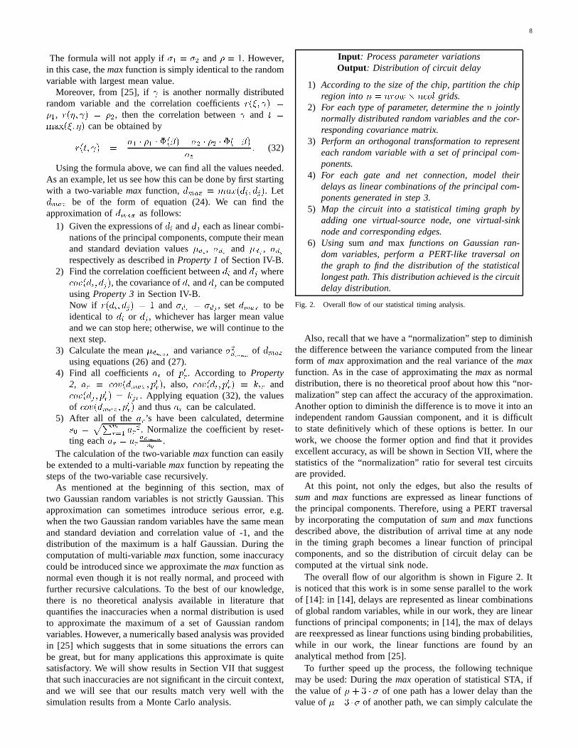
Input : Process parameter variationsOutput : Distribution of circuit delay

1) According to the size of the chip, partition the chipregion inton = nrow � n ol grids.

2) For each type of parameter, determine then jointlynormally distributed random variables and the cor-responding covariance matrix.

3) Perform an orthogonal transformation to representeach random variable with a set of principal com-ponents.

4) For each gate and net connection, model theirdelays as linear combinations of the principal com-ponents generated in step 3.

5) Map the circuit into a statistical timing graph byadding one virtual-source node, one virtual-sinknode and corresponding edges.

6) Using sum and max functions on Gaussian ran-dom variables, perform a PERT-like traversal onthe graph to find the distribution of the statisticallongest path. This distribution achieved is the circuitdelay distribution.

Fig. 2. Overall flow of our statistical timing analysis.

Also, recall that we have a “normalization” step to diminishthe difference between the variance computed from the linearform of max approximation and the real variance of themaxfunction. As in the case of approximating themaxas normaldistribution, there is no theoretical proof about how this “nor-malization” step can affect the accuracy of the approximation.Another option to diminish the difference is to move it into anindependent random Gaussian component, and it is difficultto state definitively which of these options is better. In ourwork, we choose the former option and find that it providesexcellent accuracy, as will be shown in Section VII, where thestatistics of the “normalization” ratio for several test circuitsare provided.

At this point, not only the edges, but also the results ofsum and max functions are expressed as linear functions ofthe principal components. Therefore, using a PERT traversalby incorporating the computation ofsumand max functionsdescribed above, the distribution of arrival time at any nodein the timing graph becomes a linear function of principalcomponents, and so the distribution of circuit delay can becomputed at the virtual sink node.

The overall flow of our algorithm is shown in Figure 2. Itis noticed that this work is in some sense parallel to the workof [14]: in [14], delays are represented as linear combinationsof global random variables, while in our work, they are linearfunctions of principal components; in [14], the max of delaysare reexpressed as linear functions using binding probabilities,while in our work, the linear functions are found by ananalytical method from [25].

To further speed up the process, the following techniquemay be used: During themax operation of statistical STA, ifthe value of�+ 3 � � of one path has a lower delay than thevalue of��3 �� of another path, we can simply calculate the

9

max function ignoring the former path.

D. The Utility of Principal Components

The previous sections described our statistical STA algo-rithm. The purpose of this section is to elaborate why theorthogonal transformation is needed to transform the set ofcorrelated process parameters to an uncorrelated set, and howit can simplify the problem of statistical STA consideringspatial correlations.

Let di anddj be the distributions of two gate delays. Forsimplicity, we assume that the gate lengths~Lg are the onlyspatially correlated parameters. We also assume thatdi anddj are sensitive to the same set of correlated random variablesof gate lengthsL1g; : : : ; Lng . Using equation (10),di and djcan be expressed asdi = d0i + i1L1g + : : :+ inLng ; (33)dj = d0j + j1L1g + : : :+ jnLng : (34)

Obviously, the covariance ofdi anddj is decided by the co-variance structure of~Lg. The direct calculation of ov(di; dj)is of a complicated form as in the work of [5] ov(di; dj) = nXa=1 nXb=1 ia jb ov(Lag ; Lbg): (35)

In contrast, in our method, we first perform orthogonal trans-formations on~Lg. Any elementLlg 2 ~Lg is expressed asLlg = Llg0 + al1l01g + : : :+ alml0mg : (36)

Next, by superposition we transformdi anddj to:di = d0i + ki1l01g + : : :+ kiml0mg ; (37)dj = d0j + kj1l01g + : : :+ kjml0mg : (38)

The value of ov(di; dj) can be simply computed using thecoefficients of~L0g by ov(di; dj) = Pmr=1 kirkjr in lineartime O(m). The advantage in this computation is that wedo not need know which specific parameters indi and djare correlated. In fact, consider the coefficients ofl01g in bothdi and dj , ki1 = Pnr=1 irar1 and kj1 = Pnr=1 jrar1. Itcan be seen that the covariance of gate lengths have all beenincorporated in the coefficient of the principal componentsl01g ; : : : ; l0ng . For this reason, we ensure that the computation of ov(di; dj) can actually take the correlations of gate lengthsinto consideration correctly.

The direct computation of the covariance of path delays isin a similar form. In general, the path delays are correlatedwhen the gate delays on these paths are correlated. As shownin the work of [5], the path covariances can be computed onthe basis of pair-wise gate delay covariances; however, thenumber of paths is numerous which makes it computationallydifficult to apply such a path-based method to large circuits.

In our method, with the orthogonal transformation, thecovariances of path delays are manifested as the coefficientsof the independent principal components as in the case ofcorrelated gate delays. The covariances of the paths can thenbe simply computed in linear time based on these coefficientsonly, and there is no need to worry about how the gates

on the paths are correlated or which parts are correlated.For the same reason, in this algorithm, besides the spatialcorrelations, path correlations due to reconvergence (structuralcorrelations) can also be accounted for automatically by us-ing the orthogonal transformation on the spatially correlatedparameters. However, when spatially uncorrelated parametersare involved in the computation, the structural correlations dueto these independent parameters can not be dealt with by thismethodology. The extension of the work for handling spatiallyuncorrelated parameters will be given in Section VI-B.

V. COMPUTATIONAL COMPLEXITY

We present a run time complexity analysis here to showwhich factors most greatly affect the CPU time of the algo-rithm.

The flow shown in Figure 2 can be divided into two parts:model pre-characterization (steps 1, 2 and 3) and statisticalstatic timing analysis (SSTA) (steps 4, 5 and 6). Model pre-characterization consists of construction of parameter varia-tions and grid-based spatial correlation models, and the com-putation of Principal Components (PC) for spatially correlatedparameters. The computation of PCs requires calculations ofeigenvectors and eigenvalues of the covariance matrix and itstime complexity isO(p �n3), wheren is total number of gridsdivided andp is the number of parameters considered. Whilethis step may seem to be a bottleneck of the algorithm, it isa only one-time process. Once the models of parameter vari-ations are constructed, they can be repeatedly used to analyzeany design. Meanwhile, for spatial correlated parameters,thePCs computed from the covariance matrix are only model-dependent, so that for different designs analyzed with thesame parameter model, the same set of PCs can be applied. Inother words, the step of model pre-characterization is in facta one-time library construction at early stage and thereforecan be excluded from the run time complexity analysis of thealgorithm.

The run-time of the SSTA algorithm can be divided into:

1) The time required to find the delay distribution of thegate and interconnect6: This run time depends on howmany different grids the interconnect passes throughand how many grids the gates are located in, and ingeneral these numbers are bounded by constant numbers.The run time is also proportional to the total numberof principal components, since we perform orthogonaltransformation at each wire segment of interconnect.For each random variable, the number of principalcomponents is no more than the total number of gridsn partitioned on the chip. The total number of principalcomponents is no more thanp�n. Thus, the time requiredto find the distribution of a single gate or wire can beestimated asO(p �n). If Ng is the total number of gatesandNI the number of net connections in the circuit, thetime of this part can be estimated asO(p�n�(Ng+NI)).

2) The time required to evaluate themaxfunction: The costof this operation is proportional to the number of random

6The time to characterize the sensitivities of delay on parameter variationsis excluded from this analysis.

10

variables involved in the max operation and the numberof principal components of each random variable. Themaxoperation is used at all multi-input gates and at thelast level (sink node) where the maximum circuit delayis computed. This number can be upper bounded by thetotal number of net connectionsNI in the circuit. Thus,the run time of this part isO(p � n �NI).

3) The time required to compute output transition time ateach gate output: For a gate withk > 2 inputs, it requiresk2 max operations andk � 1 sum operations, whichare constant numbers ofmax and sumoperations. Thecomputation is needed for all gates and thus the totalcost isO(p � n �Ng).

4) The time required to evaluate thesum function: Thesum operation must be performed at all gates and in-terconnects encountered during the PERT-like traversal.A singlesumoperation requiresO(n), and therefore, thetotal complexity for this part isO(p � n � (Ng +NI)).

Therefore, the run time complexity of the algorithm isO(p �n � (Ng+NI)), which isp �n times that of deterministic STA.

VI. EXTENDING THE METHOD TO HANDLE INTER-CHIP

VARIATIONS, SPATIALLY UNCORRELATED INTRA-CHIP

PARAMETERS, AND M IN-DELAY COMPUTATIONS

In this section, we will first describe how this work canbe extended to include the effect of inter-chip variations inaddition to intra-chip variations. Subsequently, we will explainhow spatially uncorrelated parameters can be incorporatedintothe current proposed algorithm. Finally, we will show howminimum delay computations can easily be incorporated intothis framework.

A. Inter-Chip Variations

In general, the process parametric variation can be modeledas Ætotal = Æinter + Æintra; (39)

whereÆinter is the inter-chip variation andÆintra is the intra-chip variation. As forÆintra, Æinter is also modeled as aGaussian random variable.

As introduced in Section I, inter-chip variation has a globaleffect on all the transistors [wires] within a single chip, andtherefore a single random variable,Æinter , can be applied toall transistors [wires] to model the effect of inter-die variation.Consequently, the covariance matrix for each type of spatiallycorrelated parameter is changed by adding to all entries avalue of�2Æinter , the variance of inter-chip parametric variation.Based on the new covariance matrices, the same statisticalSTA methodology can still be applied to compute distributionof chip delay.

B. Spatially Uncorrelated Parameters

In practice, it is observed that not all process parametersare spatially correlated. For example, the variations ofTox orNa are independent from transistor to transistor. To modelthe intra-die variation of spatially uncorrelated parameter,

a separate random variable has to be used for each gate[wire] to represent such independence, instead of a singlerandom variable for all gates [wires] in the same grid forthe spatial correlated parameters. Consequently, the timinganalysis framework introduced in previous sections must befurther extended to accommodate the spatially uncorrelatedparameters.

As an example, let us consider the case that gate oxidethicknessTox is the only spatially uncorrelated parameter.The idea described here can easily be extended to the casewhere there is more than one uncorrelated parameter. Withinter- and intra-chip variations, the variation ofTox for the ithtransistor can be expressed asÆinterTox +�T iox, whereÆinterTox isthe random variable representing for the inter-chip variationof Tox, and �T iox the intra-chip variation ofTox of theith transistor. Accordingly, the expressions for device [wire]delays are reformulated by substitutingÆinterTox + �T iox forwhere�Tox of theith transistor appears. Since the orthogonaltransformations of parameters are performed only on spatiallycorrelated parameters, the variablesÆinterTox and �T iox arepreserved in the delay expressions of linear combination ofprincipal components and either variable is independent fromthe principal components and any other random variables inthe delay expressions. The timing propagation using thesumandmaxoperators remains the same, except that after eachsumor maxoperation, the random variables for intra-die variationsof spatially uncorrelated parameters,�T iox’s, are merged intoone random variable, so that, at each arrival time, only oneindependent random variable is kept for all intra-die variationsof spatially uncorrelated parameters. It is observed that the wayof adding this independent random variable to the standardform of the representation of arrival times is similar to the“residual” variance’s lumping into the independently randompart in [26].

Although structural correlations can be automatically takeninto account using orthogonal transformation on spatiallycor-related parameters as explained in Section IV-D, the structuralcorrelations due to spatially uncorrelated parameters cannot behandled with the same technique because of the merging ofthese random variables during the propagation. To reduce theinaccuracies caused, one can appeal to the available literatureon handling structural correlations in statistical STA [7], [9],[10]. In this work, we have ignored the structural correlationscaused by the spatially uncorrelated parameters. However,since the structural correlations from spatially correlated pa-rameters are considered, the inaccuracies introduced fromthisassumption are not significant, as will be demonstrated inSection VII.

C. Distribution of the Minimum of a Set of Gaussians

In circuit performance analysis, computations such as find-ing the required arrival time (RAT) for long-path analysis,and minimum delay computations for short-path analysis (tocheck for hold time violations) require the computation ofthe minimum of a set of delays, which becomes finding thedistribution of the minimum of a set of random variables underprocess variations.

11

The procedure for calculation of maximum of a set ofGaussians can be utilized to compute the minimum of a setof Gaussian random variables,d1 � � � dl. Specifically,dmin =min(d1; :::; dl) can be computed asdmin = �max(�d1; :::;�dl); (40)

wheredi is a normally distributed random variable andmaxis the operator introduced is Section IV-C.

VII. E XPERIMENTAL RESULTS

The proposed algorithm was implemented in C++ as thesoftware package“MinnSSTA,” and tested on the edge-triggered ISCAS89 benchmark circuits by working on thecombinational logic blocks between the latches. All exper-iments were run on a Linux PC with a 2.0GHz CPU and256MB memory. We experimented with parameters of 100nmtechnologies on a 2-metal layer interconnect model. Theprocess parameters (Table I) used here are based on predictionsfrom [20], [27].

Since the computation requires physical information aboutthe locations of the gates and interconnects, all cells in thecircuit were first placed using the placement tool, Capo [28].Global routing was then performed to route all the nets in thecircuits. Depending on the size of circuit, we divided the chiparea into different sizes of grids, so that each grid contains nomore than a hundred cells. Again, due to the lack of access toreal wafer data, the covariance matrix for intra-die variationsused in this work were derived from the spatial correlationmodel used in [3] by equally splitting the variance into alllevels.

To verify the results of our methodMinnSSTA, we usedMonte Carlo (MC) simulations based on the same grid modelsfor comparison. To balance the accuracy and run time, wechose to run 10,000 iterations for the Monte Carlo simulation.

We first present the experimental results assuming that allparameters are spatially correlated while using fixed valuesfor the spatially uncorrelated parameters (Tox andNa). TableII shows a comparison of the results ofMC with thosefrom MinnSSTA. For each test case, the mean and standarddeviation (SD) values for both methods are listed. The resultsof MinnSSTAcan be seen to be very close to theMC results:the average error is�0:23% for the mean and�0:32%for the standard deviation. In Figure 3, for the largest testcase s38417, the plots of the PDF and CDF of the circuitdelay for both MinnSSTAand MC methods are provided.It is observed that the curves almost perfectly match eachother. This demonstrates the accuracy of the PCA approachfor correlated parameters, including its ability to account forstructural correlations.

Next, the results for considering the variations of the spa-tially uncorrelated parameters (Tox andNa) are given in TableIII. On average, the error is1:06% for the mean value and�4:34% for the standard deviation. In Table VIII, the99%and1% confidence points achieved byMC andMinnSSTAarealso provided and the average errors are�2:46% and�0:99%respectively. Again, for the largest test case s38417, the PDFand CDF curves of the circuit delay for bothMinnSSTAand

700 800 900 1000 1100 1200 13000

0.2

0.4

0.6

0.8

1

1.2

Delay (ps)

Pro

babi

lity

CDF Curves

700 800 900 1000 1100 1200 13000

0.01

0.02

0.03

0.04

0.05

Delay (ps)

Pro

babi

lity

PDF Curves

Fig. 3. A comparison ofMinnSSTAandMC methods (assuming fixed valuesof Tox andNa) for circuit s38417. The curve marked by the solid line denotesthe results ofMinnSSTA, while the plot marked by the starred lines denotesthe results ofMC.

MC methods are plotted in Figure 4, It can be seen that,at the range of lower and higher circuit delay values, thecircuit delay distribution computed fromMinnSSTAmatcheswell with that of the Monte-Carlo simulation, although thereare some deviations in the central portion. As mentionedin Section VI-B, some error may be introduced from thestructural correlations, which are not handled exactly in thepresence of uncorrelated intra-die components. Based on ouranalysis of the experiments, we find that the cause for thesmall error that is introduced here is primarily because ourim-plementation does not handle structural correlations betweenthe uncorrelated variables. We believe that, by appending intothe existing framework an algorithm that handles structuralcorrelation [7], [9], [10], the error of the results in TableIIIcan be further reduced.

400 600 800 1000 1200 1400 1600 18000

0.2

0.4

0.6

0.8

1

Delay (ps)

Pro

ba

bili

ty

CDF Curves

400 600 800 1000 1200 1400 1600 18000

0.01

0.02

0.03

0.04

0.05

0.06

Delay (ps)

Pro

ba

bili

ty

PDF Curves

Fig. 4. A comparison ofMinnSSTAand MC methods for circuit s38417,considering all sources of variation, some of which are spatially correlatedand some of which are not. The curve marked by the solid line denotes theresults ofMinnSSTA, while the plot marked by the starred lines denotes theresults ofMC.

In Table III, the CPU times for both methods are provided.

12

TABLE I

PARAMETERS USED IN THE EXPERIMENTS

Parameters Lg Wg Tox Na (�1017 m�3) Wint Tint HILD(nm) (nm) (nm) nmos/pmos (nm) (nm) (nm)�p 60.0 150.000 2.500 9.70000/10.04000 150.0 500.0 300.03�inter 9.0 11.250 0.250 0.72750 15.0 25.0 22.503�intra 4.5 5.625 0.125 0.36375 7.5 12.5 11.25Æxxmax + Æyymax 4.5 5.625 0.125 0.36375 7.5 12.5 11.25

TABLE II

COMPARISON RESULTS ASSUMING FIXED VALUES OFTox AND NaBenchmark Monte-Carlo (MC) MinnSSTA (MinnSSTA�MC)MC %

Name Mean(ps) SD(ps) Mean(ps) SD(ps) Mean SDs38417 988.6 91.0 985.8 90.8 -0.28% -0.22%s38584 1726.9 153.1 1720.9 151.6 -0.35% -0.98%s35932 1165.5 101.6 1162.7 101.3 -0.24% -0.30%s15850 1370.2 131.1 1367.2 129.6 -0.22% -1.14%s13207 1219.9 116.1 1217.3 116.2 -0.21% 0.09%s9234 674.6 65.4 673.7 64.8 -0.13% -0.92%s5378 413.1 38.5 411.8 38.4 -0.31% -0.26%s1196 499.9 45.8 499.3 46.2 -0.12% 0.87%s27 102.5 9.9 102.3 9.9 -0.20% 0.00%

TABLE III

COMPARISON RESULTS OF THE PROPOSED METHOD ANDMONTE-CARLO SIMULATION METHOD

Benchmark Monte-Carlo (MC) MinnSSTA (MinnSSTA�MC)MC %Name #Cells #Grids Mean(ps) SD(ps) CPU-time(s) Mean(ps) SD(ps) CPU-time(s) PCA-time(s) Mean SDs38417 23815 256 995.6 130.3 21005 1022.0 125.4 406.11 0.15 2.65% -3.76%s38584 20705 256 1738.4 226.4 24039 1798.2 215.6 460.36 0.15 3.44% -4.77%s35932 17793 256 1214.7 161.8 53922 1251.2 144.7 505.71 0.15 3.00% -10.57 %s15850 10369 256 1388.2 178.9 8856 1397.8 172.1 175.96 0.15 0.69% -3.80%s13207 8260 256 1230.7 158.8 9060 1239.7 154.9 172.62 0.15 0.73% -2.46%s9234 5825 64 688.6 90.6 5346 690.6 85.2 32.23 0.02 0.29% -5.96%s5378 2958 64 421.1 54.3 3907 420.8 51.8 27.41 0.02 -0.07% -4.60%s1196 547 16 505.9 66.0 781 502.7 64.4 1.51 0.01 -0.63% -2.42%s27 13 4 103.6 13.7 9 103.0 13.6 0.00 0.00 -0.58% -0.73%

To show that the PCA steps require very little run time, therun time for this part is also listed; however, as pointed outearlier, this can be considered a preprocessing step that iscarried out once for each technology, and its cost need notbe considered in the computation. We can see that the CPUtime of MinnSSTAon all test cases is very fast. The circuitwith the longest run time, s35932, was analyzed in only about500 seconds, while theMC simulation required over15 hours.

In the proposed approach, in order to make the computedvalue of standard deviation ofdmax the same as that of theapproximated linear expression, the coefficients of parametersin the linear expression are normalized by the ratio of thestandard deviation ofdmax (namely,�dmax ) to that of thelinear expressions0. In Table IV, the statistics of this ratio forall testcases are listed, including the mean, standard deviation,minimum and maximum values of the ratio and the probabilityof the ratio falls into each given range. In general, the higherthe ratio, the larger the error for estimatingdmax, and thus theless accurate for estimating the circuit delay distribution usingthe proposed approach. For example, the testcases35932 hasthe highest probability of 0.045 for the ratio to be greater than1.1, and also has the largest errors predicting the circuit meanand standard deviation. Over all testcases, the average valueof the ratio is 1.003, which is a reasonably small number sothat the accuracy of the proposed statistical SSTA should notbe affected significantly by this normalization step.

To further verify the applicability of the proposed algorithm,

we have demonstrated it on a path-balanced circuit whosetopology is a binary tree of depth10. Table V lists the resultsachieved byMinnSSTAand (MC). The errors obtained are�0:54% for the mean and�6:26% for the standard devia-tion; �4:56% and�1:65% for the 99% and 1% confidencepoint, respectively. This shows that the proposed approachcanpredict the timing yield well, even for path-balanced circuits.

One may ask what happens if a Monte-Carlo approach wasrun for the same amount of time as the proposed algorithm.In Table VI, we show the data achieved from Monte-Carloruns in the equivalent CPU-time of the proposed method”MinnSSTA”. Since this Monte-Carlo simulation can only runa small number of iterations and samples the soluton spaceinsufficiently, it does not meet any of the usual convergencecriteria used for Monte Carlo analysis. Therefore, what isachieved is not the genuine distribution of circuit delay, butmerely the distribution from an incomplete number of runs.The table shows the minimum values and maximum valuesof the circuit delay from this insufficient number of Monte-Carlo runs, and, for purposes of comparison, the results withthe 1% and 99% confidence points, respectively, from the10,000 iterations of Monte-Carlo simulation. It can be seenthat the accuracy is highly variable: in some cases, MonteCarlo analysis comes close to the action value, while in others,it is very far away. Most notably, large deviations can be seenboth for a small circuit (s27) and a large circuit (s38584),

13

TABLE IV

STATISTICS OF RATIO OF STANDARD DEVIATION OF ACCURATE VALUE�dmax TO s0 OF THE LINEAR EXPRESSION.

Circuit Ratio of�dmax to s0 Probability of the ratio in each rangeName mean stdev minimum maximum < 1 = 1 (1; 1:01) [1:01; 1:1℄ > 1:1s38417 1.0031 0.0051 � 1 1.0262 0.0004 0.3246 0.5582 0.1168 0s38584 1.0037 0.0054 � 1 1.1804 0.0023 0.4124 0.1700 0.0001 0s35932 1.0120 0.0278 � 1 1.1583 0.0022 0.2883 0.4290 0.2350 0.0454s15850 1.0018 0.0033 � 1 1.0233 0.0034 0.4029 0.5538 0.0398 0s13207 1.0028 0.0048 � 1 1.0260 0.0008 0.3256 0.5843 0.0893 0s9234 1.0017 0.0035 1 1.0209 0 0.3825 0.5636 0.0538 0s5378 1.0012 0.0023 1 1.0289 0 0.4310 0.5563 0.0126 0s1196 1.0007 0.0021 � 1 1.0150 0.0021 0.7068 0.2764 0.0148 0s27 1.0006 0.0014 1 1.0030 0 0.8 0.2000 0 0

TABLE V

EXPERIMENTAL RESULTS ON A BINARY TREE CIRCUIT OF DEPTH-10

Approach Mean(ps) SD(ps) 99% Point(ps) 1% Point(ps)MC 669.8 86.2 894.8 486.3

MinnSSTA 666.2 80.8 854.0 478.3(MinnSSTA�MC)MC % �0:54% �6:26% �4:56% �1:65%implying that the reliability of such an approach is suspect. Ofcourse, this is not surprising in the least, because the artificiallimitation on the run time has made the Monte Carlo analysisunreliable, by permitting only a low point of confidence forits predictions, and has not permitted it to fully sample thesearch space.

400 600 800 1000 1200 1400 1600 18000

0.2

0.4

0.6

0.8

1

Delay (ps)

Pro

ba

bili

ty

CDF Curves

400 600 800 1000 1200 1400 1600 18000

0.02

0.04

0.06

0.08

Delay (ps)

Pro

ba

bili

ty

PDF Curves

Fig. 5. A comparison of statistical STA with and without considering spatialcorrelations, under Monte Carlo analysis, for circuit s38417. The curve markedby the solid line denotes the case where spatial correlations are ignored, whilethe curve with the starred lines denotes the results of incorporating spatialcorrelations; this is identical to the curve in Figure 4.

To show the importance of considering spatial correlations,we consider the difference between performing statisticaltiming analysis while considering spatial correlation andwhileignoring it. Since this is a comparison to determine whyspatial correlations are important, the CPU time is not aconsideration. Therefore, we run another set of Monte Carlosimulations (MCNoCorr) on the same set of benchmarks, thistime assuming zero correlations among the devices and wireson the chip. The comparison between the data is shown inTable VII. It can be observed that although the mean values areclose, the variances of the uncorrelated cases (MCNoCorr) aremuch smaller than the correlated cases (MC). On average, the

standard deviation of the correlated case increases by25:93%.Again, we plot the PDF and CDF curves of both simulationsfor circuit s38417 in Figure 5. It is seen that the CDF and PDFcurves ofMCNoCorr deviate significantly from those ofMC.In other words, statistical timing analysis without consideringcorrelation may incorrectly predict the real performance ofthe circuit and could even overestimate the performance ofthe circuit. This underlines the importance of developingefficient statistical STA methods that can incorporate spatialcorrelations.

As an alternative, we consider the option of using multipleprocess corners (MPC) for these experiments, where the circuitdelays are evaluated at all possible corners of parameter valuesat��3��, where� is the mean and� the standard deviation forthe parameter. Table VIII compares the worst-case and best-case delays obtained at exhaustive process corners using theMPC method, with the99% and 1% confidence point delayachieved from the Monte-Carlo simulation (MC) accordingly.On average, theMPC approach overestimates the worst-casedelay of circuit by30:81% and underestimates the best-casedelay by28:08%. These results also emphasize the importanceof considering spatial correlations during statistical STA, as isdone by our algorithm.

VIII. C ONCLUSION AND FUTURE WORK

In this paper, we have proposed an algorithm for performingstatistical STA, considering spatial correlations related to intra-chip process variations. We show that performing statisticaltiming analysis while ignoring spatial correlations may not beadequate to predict the circuit performance correctly, andthatfast and accurate statistical STA methods, such as ours, thatincorporate spatial correlations are essential. An analysis of thecomplexity shows it to be reasonable, and like conventionalSTA, it is linear in the number of gates and interconnects. Thepenalty that is paid here is that unlike deterministic STA, it isalso linear in the number of grid squares. As a trivial extensionof maximum of delays, the computation for the distribution ofminimum of delays is also provided.

14

TABLE VI

COMPARISON OFMONTE-CARLO IN EQUIVALENT CPU-TIME OF M INNSSTAWITH THAT OF 10,000RUNS (MC)

Circuit Minimum Delay MC: 1%pt (ps) mindelay�1%pt1%pt % Maximum delay MC: 99%pt (ps) maxdelay�99%pt99%pt %Name #runs delay (ps) (10; 000runs) #runs delay (ps) (10; 000runs)s38417 170 725.0 722.0 0.42% 170 1372.8 1333.3 2.96%s38584 180 1205.7 1261.3 -4.41% 180 2794.3 2310.3 20.95%s35932 100 847.3 882.3 -3.97% 100 1650.0 1635.2 0.91%s15850 175 994.4 1012.9 -1.82% 175 1880.6 1844.8 1.94%s13207 190 887.8 893.1 -0.59% 190 1728.1 1629.9 6.02%s9234 60 452.3 499.7 -9.49% 60 884.1 922.6 -4.17%s5378 50 306.0 308.9 -0.92% 50 534.3 559.9 -4.58%s1196 16 441.7 370.4 19.26% 16 637.8 673.4 -5.29%s27 10 350.0 74.9 367.30% 10 653.8 138.4 372.37%

TABLE VII

COMPARISON OF TIMING ANALYSIS WITH AND WITHOUT SPATIAL CORRELATIONS

Benchmark Anal. w/ corr. (MC) Anal. w/o corr. (MCNoCorr) (MC�MCNoCorr)MCNoCorr %Name Mean(ps) SD(ps) Mean(ps) SD(ps) Mean SDs38417 995.6 130.3 996.7 98.7 0.11% -24.25%s38584 1738.4 226.4 1741.9 180.5 0.20% -20.27%s35932 1214.7 161.8 1253.6 140.0 3.20% -13.47%s15850 1388.2 178.9 1393.8 121.9 0.40% -31.86%s13207 1230.7 158.8 1233.8 110.2 0.25% -30.60%s9234 688.6 90.6 691.9 61.9 0.48% -31.68%s5378 421.1 54.3 424.7 38.2 0.85% -29.65%s1196 505.9 66.0 507.6 48.8 0.34% -26.06%s27 103.6 13.7 103.7 10.2 0.10% -25.55%

TABLE VIII

COMPARISON OF99% AND 1% CONFIDENCE POINT

Bench. MC MinnSSTA (MinnSSTA�MC)MC % MPC (MPC�MC)MC %Name 99% Pt.(ps) 1% Pt.(ps) 99% Pt.(ps) 1% Pt.(ps) 99% Pt.(ps) 1% Pt.(ps) Worst-Case Best-Case Worst-Case Best-Cases38417 1333.3 722 1313.6 730.4 -1.48% 1.16% 1758.1 522.1 31.86% -27.69%s38584 2310.3 1261.3 2299.5 1296.9 -0.47% 2.82% 3056.0 915.4 32.28% -27.42%s35932 1635.2 882.3 1587.6 914.8 -2.91% 3.68% 2051.2 613.0 25.44% -30.52%s15850 1844.8 1012.9 1797.9 997.7 -2.54% -1.50% 2442.9 725.2 32.42% -28.40%s13207 1629.9 893.1 1599.8 879.6 -1.85% -1.51% 2175.4 646.6 33.47% -27.60%s9234 922.6 499.7 888.7 492.5 -3.67% -1.44% 1207.3 359.7 30.86% -28.02%s5378 559.9 308.9 541.2 300.4 -3.34% -2.75% 736.6 219.2 31.56% -29.04%s1196 673.4 370.4 652.4 353.0 -3.12% -4.70% 874.2 265.8 29.82% -28.24%s27 138.4 74.9 134.6 71.4 -2.75% -4.67% 179.3 55.6 29.55% -25.77%

The current algorithm is limited by the following: it assumesthat the distribution of parameter variations are Gaussianandthe distribution of gate [wire] delays have linear dependencyon the variation of process parameters. A good direction forfuture research involves solving the problem of statisticaltiming analysis on non-Gaussian process parameter variationsand nonlinear delay dependencies.

ACKNOWLEDGMENTS

The authors would like to thank the anonymous reviewers,whose comments provided excellent feedback, resulting in animprovement in the quality of our paper.

REFERENCES

[1] S. Nassif, “Design for variability in DSM technologies,” in Proceedingsof the IEEE International Symposium on Quality of Electronic Design,San Jose, California, USA, Mar. 2000, pp. 451–454.

[2] V. Axelrad and J. Kibarian, “Statistical aspects of modern IC designs,”in Proceedings of the 28th European Solid-State Device ResearchConference, Bordeaux, France, Sept. 1998, pp. 309–321.

[3] A. Agarwal, D. Blaauw, V. Zolotov, S. Sundareswaran, M. Zhao,K. Gala, and R. Panda, “Statistical delay computation considering spatialcorrelations,,” in Proceedings of the Asia and South Pacific DesignAutomation Conference, Kitakyushu, Japan, Jan. 2003, pp. 271–276.

[4] M. Berkelaar, “Statistical delay calculation, a lineartime method,”(Personal communication).

[5] M. Orshansky and K. Keutzer, “A general probabilistic framework forworst case timing analysis,” inProceedings of the ACM/IEEE DesignAutomation Conference, New Orleans, Louisiana, USA, June 2002, pp.556–561.

[6] S. Tsukiyama, M. Tanaka, and M. Fukui, “A statistical static timinganalysis considering correlations between delays,” inProceedings ofthe Asia and South Pacific Design Automation Conference, Yokohama,Japan, Jan. 2001, pp. 353–358.

[7] A. Agarwal, D. Blaauw, V. Zolotov, and S. Vrudhula, “Computation andrefinement of statistical bounds on circuit delay,” inProceedings of theACM/IEEE Design Automation Conference, Anaheim, California, USA,June 2003, pp. 348–353.

[8] J. Liou, K. Cheng, S. Kundu, and A. Krstic, “Fast statistical timinganalysis by probabilistic event propagation,” inProceedings of theACM/IEEE Design Automation Conference, Las Vegas, Nevada, USA,June 2001, pp. 661–666.

[9] S. Naidu, “Timing yield calculation using an impulse-train approach,”in Proceedings of the 15th International Conference on VLSI Design,Bangalore, India, Jan. 2002, pp. 219–224.

[10] A. Devgan and C. Kashyap, “Block-based static timing analysis withuncertainty,” inProceedings of the IEEE/ACM International Conferenceon Computer Aided Design, San Jose, California, USA, Nov. 2003, pp.607–614.

[11] S. Bhardwaj, S. Vrudhula, and D. Blaauw, “TAU: Timing analysis underuncertainty,” inProceedings of the ACM/IEEE International Conferenceon Computer Aided Design, San Jose, California, USA, Nov. 2003, pp.615–620.

[12] J. Liou, A. Krstic, L. Wang, and K. Cheng, “False-path-aware statis-

15

tical timing analysis and efficient path selection for delaytesting andtiming validation,” inProceedings of the ACM/IEEE Design AutomationConference, New Orleans, Louisiana, USA, June 2002, pp. 566–569.

[13] B. Choi and D. M. H. Walker, “Timing analysis of combinationalcircuits including capacitive coupling and statistical process variation,”in Proceedings of the IEEE VLSI Test Symposium, Montreal, Canada,Apr. 2000, pp. 49–54.

[14] J. Jess, K. Kalafala, S. Naidu, R. Otten, and C. Visweswariah, “Statisticaltiming for parametric yield prediction of digital untegrated circuits,” inProceedings of the ACM/IEEE Design Automation Conference, Ana-heim, California, USA, June 2003, pp. 932–937.

[15] A. Agarwal, D. Blaauw, and V. Zolotov, “Statistical timing analysis forintra-die process variations with spatial correlations,”in Proceedings ofthe IEEE/ACM International Conference on Computer Aided Design,San Jose, California, USA, Nov. 2003, pp. 900–907.

[16] S. Sapatnekar,Timing. Boston, MA: Kluwer Academic Publishers,2004.

[17] T. Kirkpatrick and N. Clark, “PERT as an aid to logic design,” IBMJournal of Research and Development, vol. vol. 10, pp. 135–141, June1966.

[18] Y. Liu, S. Nassif, L. Pileggi, and A. Strojwas, “Impact of interconnectvariations on the clock skew of a gigahertz microprocessor,” in Proceed-ings of the ACM/IEEE Design Automation Conference, Los Angeles,California, USA, June 2000, pp. 168–171.

[19] M. Orshansky, L. Milor, P. Chen, K. Keutzer, and C. Hu, “Impact ofspatial intrachip gate length variability on the performance of high-speed digital circuits,”IEEE Transactions on Computer-Aided Designof Integrated Circuits and Systems, vol. 21, pp. 544–553, May 2002.

[20] S. Nassif, “Delay variability: Sources, impact and trends,” in Pro-ceedings of IEEE International Solid-State Circuits Conference, SanFrancisco, California, USA, Feb. 2000, pp. 368–369.

[21] B. Stine, D. Boning, and J. Chung, “Analysis and decomposition ofspatial variation in integrated circuit processes and devices,” IEEETransaction on Semiconductor Manufacturing, vol. vol. 10, pp. 24–41,Feb. 1997.

[22] D. Boning, J. Panganiban, K. Gonzalez-Valentin, S. Nassif, C. Mc-Dowell, A. Gattiker, and F. Liu, “Test structures for delay variability,”(Personal communication).

[23] D. Morrison, Multivariate Statistical Methods. New York, NY:McGraw-Hill, 1976.

[24] E. Jacobs and M. Berkelaar, “Gate sizing using a statistical delay model,”in Proceedings of Design Automation and Test in Europe, 2000, pp. 283–290.

[25] C. Clark, “The greatest of a finite set of random variables,” OperationsResearch, vol. 9, pp. 85–91, 1961.

[26] C. Visweswariah, K. Ravindran, K. Kalafala, S. G. Walker, andS. Narayan, “First-order incremental block-based statistical timing anal-ysis,” in Proceedings of the ACM/IEEE Design Automation Conference,San Diego, California, USA, June 2004, pp. 331–336.

[27] J. Cong, “Challenges and opportunities for design innovations innanometer technologies,” (Available at: http://ballade.cs.ucla.edu/�cong/papers/final1.pdf), Dec. 1997, semiconductor Research Corporation De-sign Sciences Concept Paper.

[28] “Capo: A large-scale fixed-die placer from UCLA,” Available at: http://vlsicad.ucsd.edu/GSRC/bookshelf/Slots/Placement.

Hongliang Chang received the B.E. degree fromQiqihar University, and the M. S. degree from Uni-versity of Minnesota in 1996 and 2001 respectively.She is currently pursuing her Ph.D. at the Depart-ment of Computer Science and Engineering at theUniversity of Minnesota.

Sachin S. Sapatnekarreceived the B.Tech. degreefrom the Indian Institute of Technology, Bombayin 1987, the M.S. degree from Syracuse Universityin 1989, and the Ph.D. degree from the Universityof Illinois at Urbana-Champaign in 1992. From1992 to 1997, he was an assistant professor in theDepartment of Electrical and Computer Engineeringat Iowa State University. He is currently the Robertand Marjorie Henle Professor in the Department ofElectrical and Computer Engineering at the Univer-sity of Minnesota.

He is an author of four books and a coeditor of one volume, and haspublished mostly in the areas of timing and layout. He has held positions onthe editorial board of the IEEE Transactions on VLSI Systems, and the IEEETransactions on Circuits and Systems II, the IEEE Transactions on CAD,andhas been a Guest Editor for the latter. He has served on the Technical ProgramCommittee for various conferences, and as Technical Program and GeneralChair for the Tau workshop and for the International Symposium on PhysicalDesign. He has been a Distinguished Visitor for the IEEE Computer Societyand a Distinguished Lecturer for the IEEE Circuits and Systems Society. Heis a recipient of the NSF Career Award, three best paper awards at DAC andone at ICCD, and the SRC Technical Excellence award. He is a fellow of theIEEE.