Statistical tests for categorical variables - ksumsc.com · Fisher’s Exact Test: The method of...
53
Statistical tests to observe the statistical significance of qualitative variables (Z-test, Chi-square, Fisher’s exact & Mac Nemar’s chi-square tests) Dr.Shaikh Shaffi Ahamed Ph.D., Professor Dept. of Family & Community Medicine
Transcript of Statistical tests for categorical variables - ksumsc.com · Fisher’s Exact Test: The method of...
Statistical tests to observe the statistical
significance of qualitative variables (Z-test,
Chi-square, Fisher’s exact & Mac Nemar’s
chi-square tests)
Dr.Shaikh Shaffi Ahamed Ph.D.,
Professor
Dept. of Family & Community Medicine
Learning Objectives:
(1) Able to understand the factors to
apply for the choice of statistical tests in
analyzing the data .
(2) Able to apply appropriately Z-test,
Chi-square test, Fisher’s exact test &
Macnemar’s Chi-square test.
(3) Able to interpret the findings of the
analysis using these four tests.
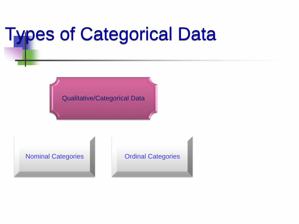
Types of Categorical Data
Qualitative/Categorical Data
Nominal Categories Ordinal Categories
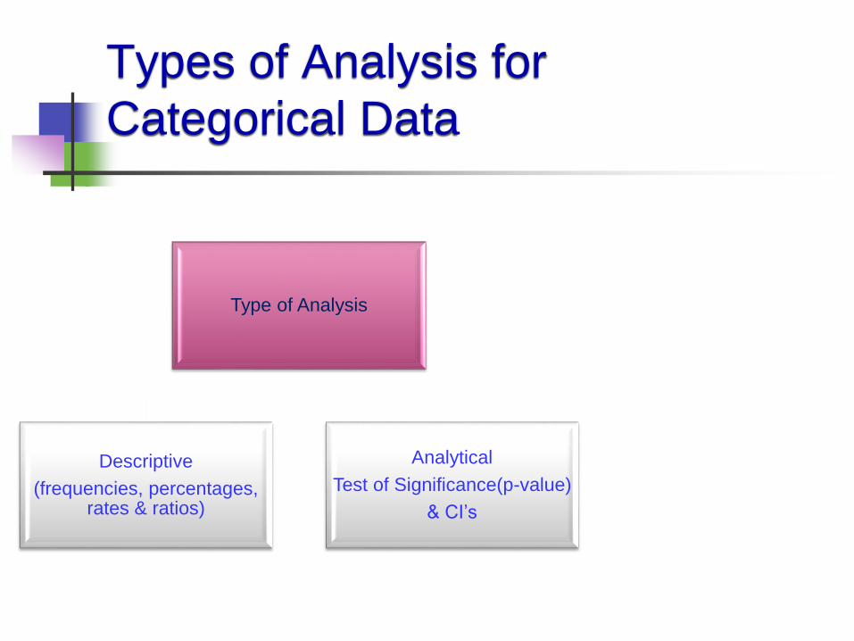
Types of Analysis for
Categorical Data
Type of Analysis
Descriptive
(frequencies, percentages, rates & ratios)
Analytical
Test of Significance(p-value)
& CI’s
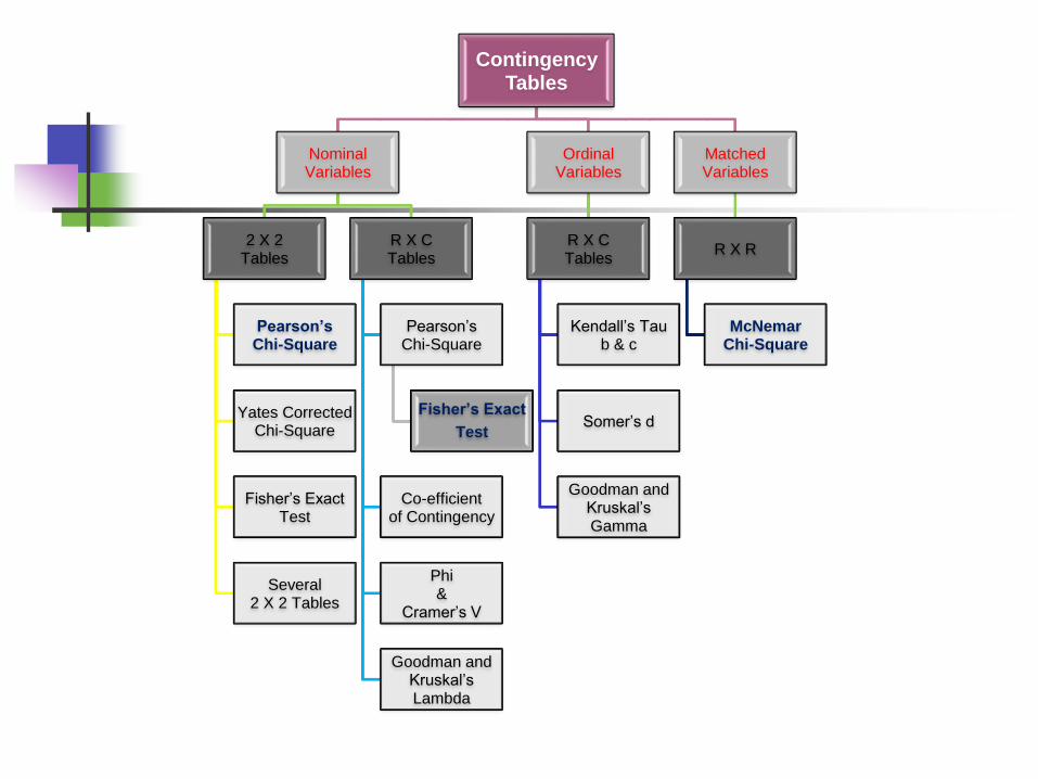
Contingency Tables
Nominal Variables
2 X 2Tables
Pearson’sChi-Square
Yates CorrectedChi-Square
Fisher’s ExactTest
Several 2 X 2 Tables
R X CTables
Pearson’sChi-Square
Fisher’s Exact
Test
Co-efficientof Contingency
Phi &
Cramer’s V
Goodman and Kruskal’sLambda
Ordinal Variables
R X CTables
Kendall’s Tau b & c
Somer’s d
Goodman and Kruskal’sGamma
Matched Variables
R X R
McNemar Chi-Square
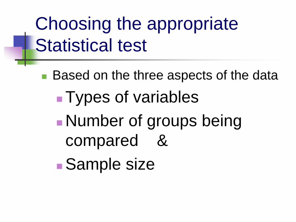
Choosing the appropriate
Statistical test
Based on the three aspects of the data
Types of variables
Number of groups being
compared &
Sample size
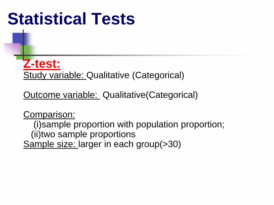
Statistical Tests
Z-test:Study variable: Qualitative (Categorical)
Outcome variable: Qualitative(Categorical)
Comparison:(i)sample proportion with population proportion;
(ii)two sample proportionsSample size: larger in each group(>30)
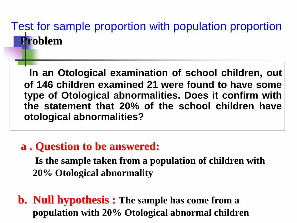
Test for sample proportion with population proportion
In an Otological examination of school children, out
of 146 children examined 21 were found to have sometype of Otological abnormalities. Does it confirm withthe statement that 20% of the school children haveotological abnormalities?
a . Question to be answered:
Is the sample taken from a population of children with
20% Otological abnormality
b. Null hypothesis : The sample has come from a
population with 20% Otological abnormal children
Problem
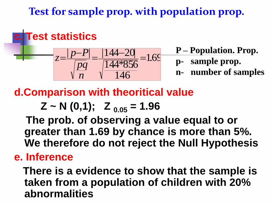
c. Test statistics
d.Comparison with theoritical value
Z ~ N (0,1); Z 0.05 = 1.96
The prob. of observing a value equal to or greater than 1.69 by chance is more than 5%. We therefore do not reject the Null Hypothesis
e. Inference
There is a evidence to show that the sample is taken from a population of children with 20% abnormalities
69.1
1466.85*4.14|204.14|||
npqPp
z
Test for sample prop. with population prop.
P – Population. Prop.
p- sample prop.
n- number of samples
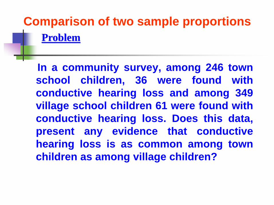
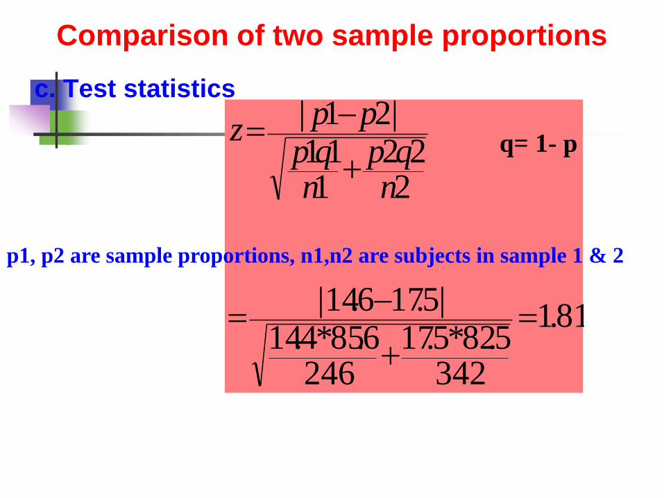
Comparison of two sample proportions
In a community survey, among 246 town
school children, 36 were found with
conductive hearing loss and among 349
village school children 61 were found with
conductive hearing loss. Does this data,
present any evidence that conductive
hearing loss is as common among town
children as among village children?
Problem
Comparison of two sample proportions
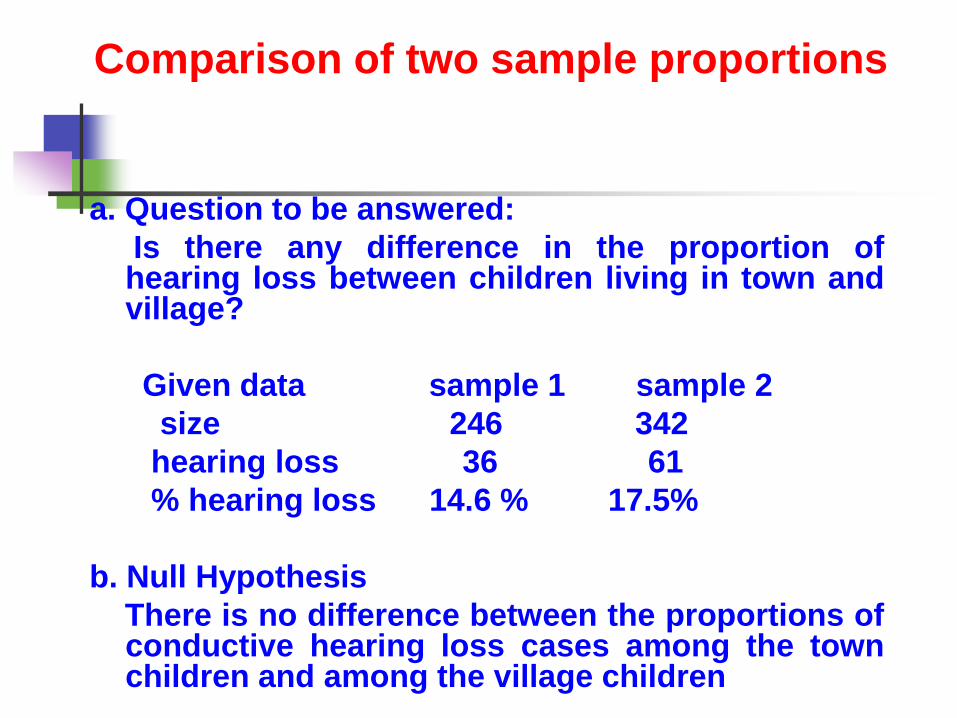
a. Question to be answered:
Is there any difference in the proportion ofhearing loss between children living in town andvillage?
Given data sample 1 sample 2
size 246 342
hearing loss 36 61
% hearing loss 14.6 % 17.5%
b. Null Hypothesis
There is no difference between the proportions ofconductive hearing loss cases among the townchildren and among the village children
Comparison of two sample proportions
c. Test statistics
81.1
3425.82*5.17
2466.85*4.14
|5.176.14|
222
111
|21|
nqp
nqp
ppz
p1, p2 are sample proportions, n1,n2 are subjects in sample 1 & 2
q= 1- p
Comparison of two sample proportions
d. Comparison with theoretical value
Z ~ N (0,1); Z 0.05 = 1.96
The prob. of observing a value equal to orgreater than 1.81 by chance is more than 5%.We therefore do not reject the Null Hypothesis
e. Inference
There is no evidence to show that the twosample proportions are statisticallysignificantly different. That is, there is nostatistically significant difference in theproportion of hearing loss between villageand town, school children.
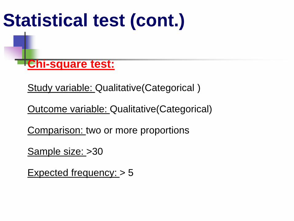
Statistical test (cont.)
Chi-square test:
Study variable: Qualitative(Categorical )
Outcome variable: Qualitative(Categorical)
Comparison: two or more proportions
Sample size: >30
Expected frequency: > 5
Chi-square testPurpose
To find out whether the association between two
categorical variables are statistically significant
Null Hypothesis
There is no association between two variables
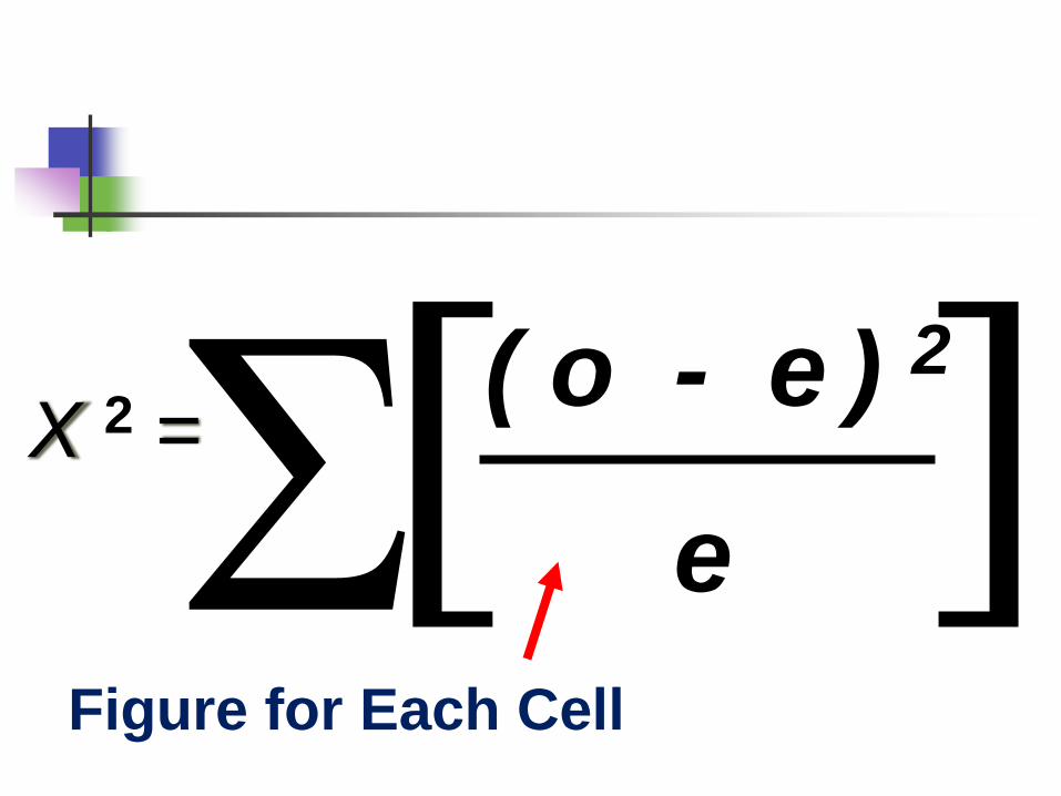
( o - e ) 2
e
X 2 =
Figure for Each Cell
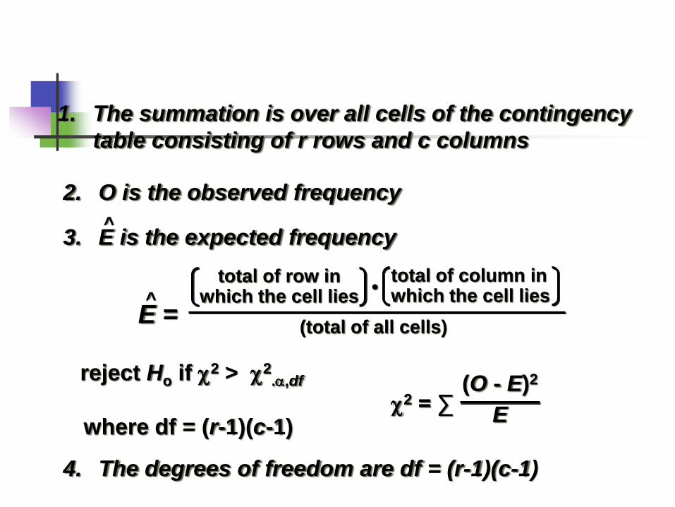
reject Ho if 2 > 2.,df
where df = (r-1)(c-1)2 = ∑
(O - E)2
E
3. E is the expected frequency^
E =^
(total of all cells)
total of row inwhich the cell lies
total of column inwhich the cell lies•
1. The summation is over all cells of the contingency
table consisting of r rows and c columns
2. O is the observed frequency
4. The degrees of freedom are df = (r-1)(c-1)
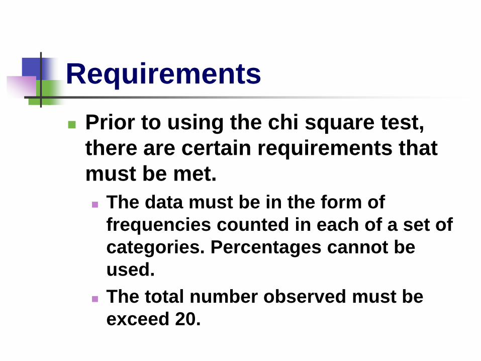
Requirements
Prior to using the chi square test,
there are certain requirements that
must be met.
The data must be in the form of
frequencies counted in each of a set of
categories. Percentages cannot be
used.
The total number observed must be
exceed 20.
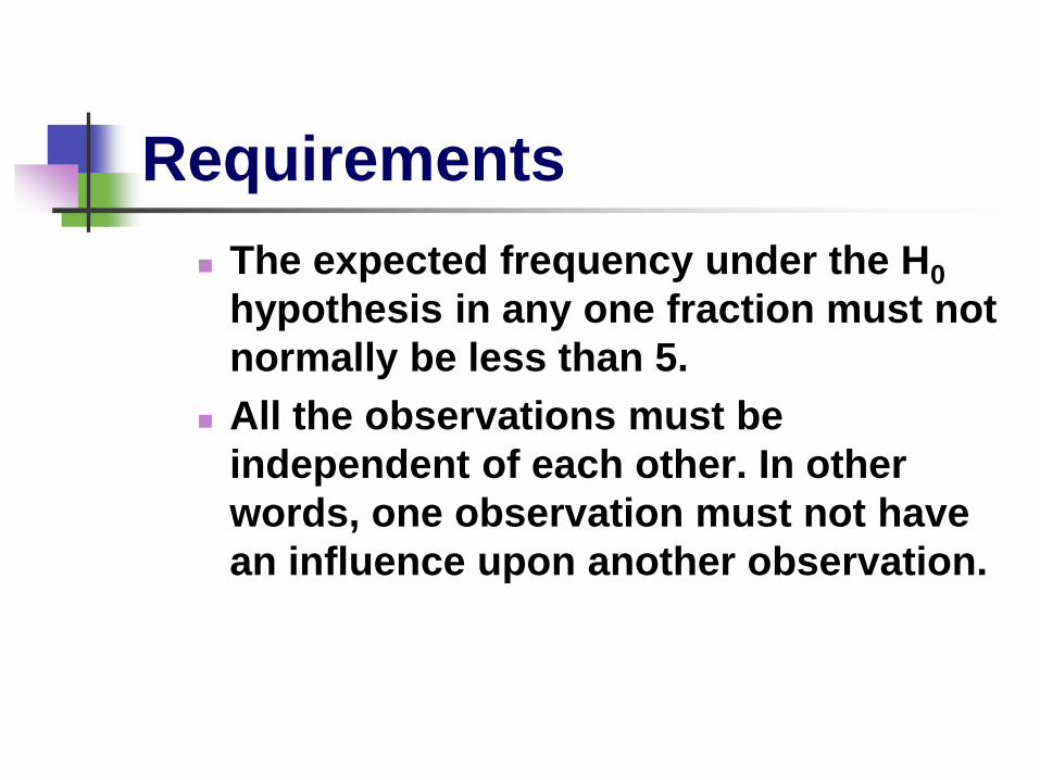
Requirements
The expected frequency under the H0
hypothesis in any one fraction must not
normally be less than 5.
All the observations must be
independent of each other. In other
words, one observation must not have
an influence upon another observation.
APPLICATION OF CHI-SQUARE TEST
TESTING INDEPENDCNE (or
ASSOCATION)
TESTING FOR HOMOGENEITY
TESTING OF GOODNESS-OF-FIT
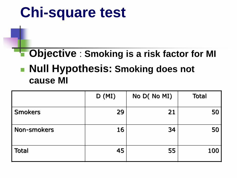
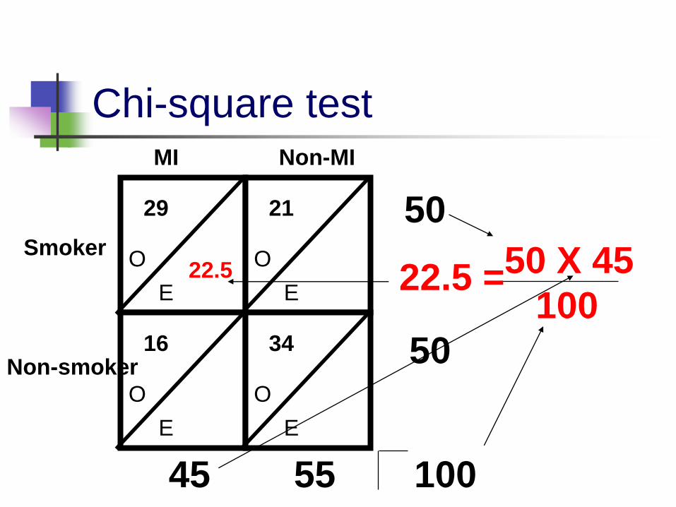
Chi-square test
Objective : Smoking is a risk factor for MI
Null Hypothesis: Smoking does not
cause MI
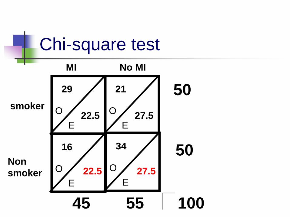
D (MI) No D( No MI) Total
Smokers 29 21 50
Non-smokers 16 34 50
Total 45 55 100
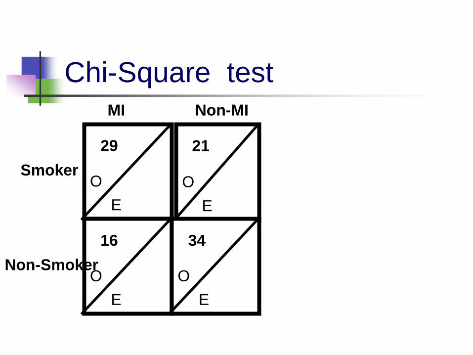
E
O
29
E
O
21
E
O
16
E
O
34
MI Non-MI
Smoker
Non-Smoker
Chi-Square test
E
O
29
E
O
21
E
O
16
E
O
34
MI Non-MI
Smoker
Non-smoker
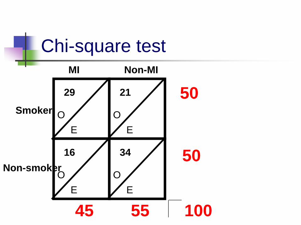
50
50
5545 100
Chi-square test
E
O
29
E
O
21
E
O
16
E
O
34
MI Non-MI
Smoker
Non-smoker
50
50
5545 100
50 X 45
10022.5 =22.5
Chi-square test
E
O
29
E
O
21
E
O
16
E
O
34
MI No MI
smoker
Non
smoker
50
50
5545 100
22.5 27.5
22.5 27.5
Chi-square test
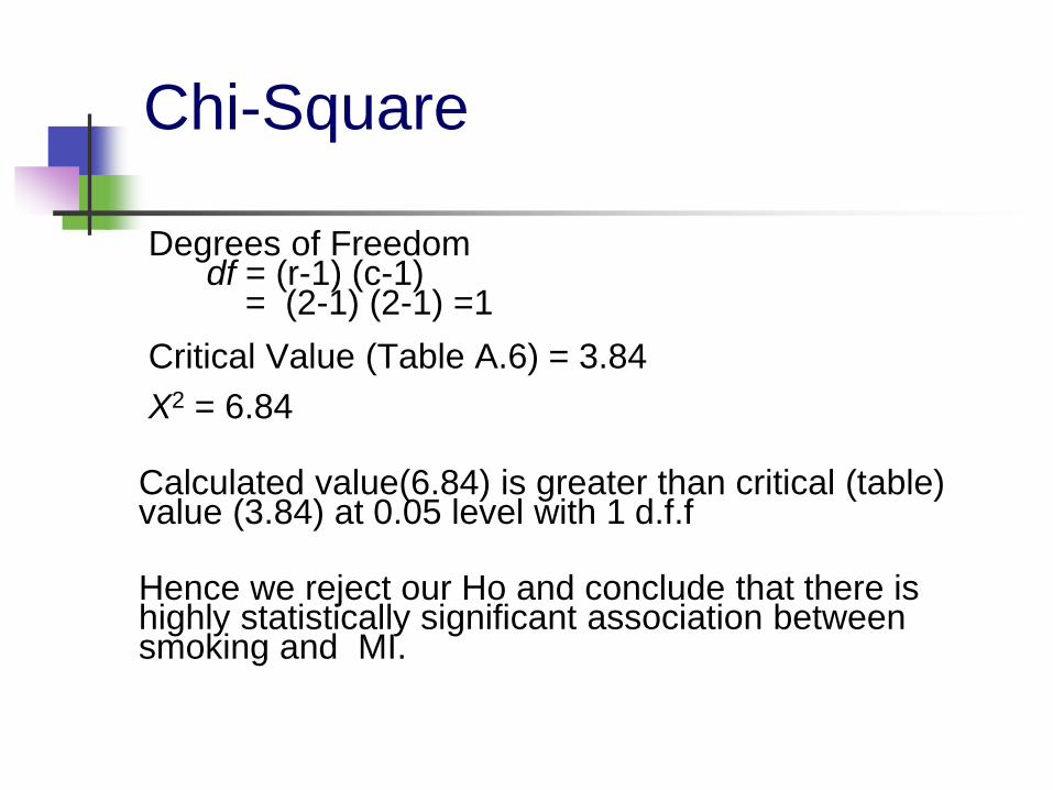
Degrees of Freedomdf = (r-1) (c-1)
= (2-1) (2-1) =1
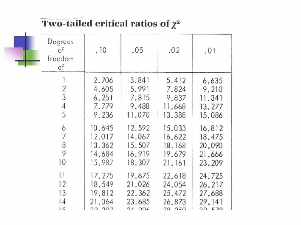
Critical Value (Table A.6) = 3.84
X2 = 6.84
Calculated value(6.84) is greater than critical (table) value (3.84) at 0.05 level with 1 d.f.f
Hence we reject our Ho and conclude that there is highly statistically significant association between smoking and MI.
Chi-Square
Association between Diabetes and Heart
Disease?
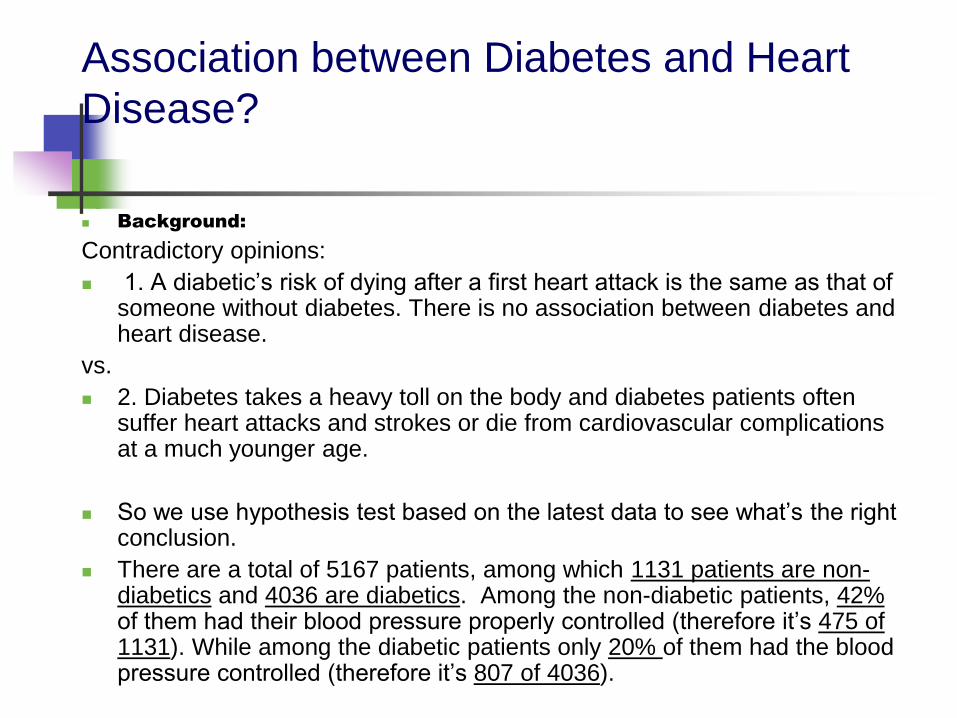
Background:
Contradictory opinions:
1. A diabetic’s risk of dying after a first heart attack is the same as that of someone without diabetes. There is no association between diabetes and heart disease.
vs.
2. Diabetes takes a heavy toll on the body and diabetes patients often suffer heart attacks and strokes or die from cardiovascular complications at a much younger age.
So we use hypothesis test based on the latest data to see what’s the right conclusion.
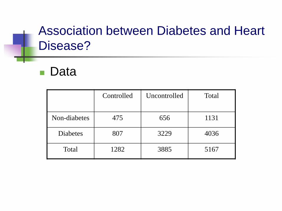
There are a total of 5167 patients, among which 1131 patients are non-diabetics and 4036 are diabetics. Among the non-diabetic patients, 42%of them had their blood pressure properly controlled (therefore it’s 475 of 1131). While among the diabetic patients only 20% of them had the blood pressure controlled (therefore it’s 807 of 4036).
Association between Diabetes and Heart
Disease?
Data
Controlled Uncontrolled Total
Non-diabetes 475 656 1131
Diabetes 807 3229 4036
Total 1282 3885 5167
Association between Diabetes and Heart
Disease?
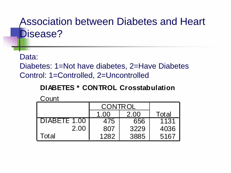
Data:
Diabetes: 1=Not have diabetes, 2=Have Diabetes
Control: 1=Controlled, 2=Uncontrolled
DIABETES * CONTROL Crosstabulation
Count
475 656 1131807 3229 4036
1282 3885 5167
1.002.00
DIABETES
Total
1.00 2.00CONTROL
Total
Association between Diabetes and Heart
Disease?
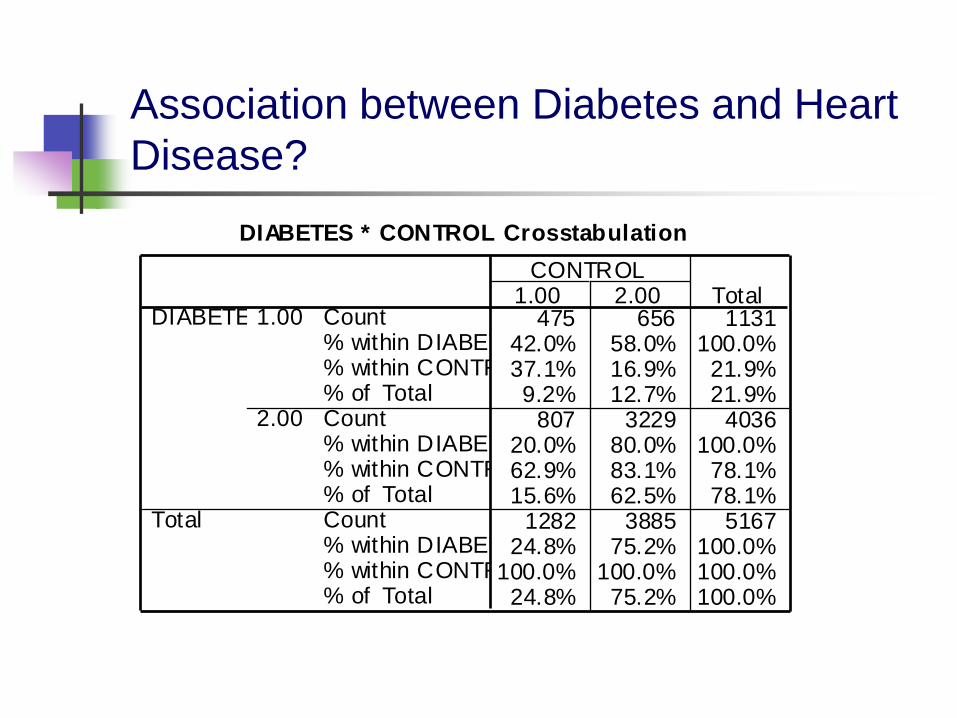
DIABETES * CONTROL Crosstabulation
475 656 113142.0% 58.0% 100.0%37.1% 16.9% 21.9%9.2% 12.7% 21.9%
807 3229 403620.0% 80.0% 100.0%62.9% 83.1% 78.1%15.6% 62.5% 78.1%
1282 3885 516724.8% 75.2% 100.0%
100.0% 100.0% 100.0%24.8% 75.2% 100.0%
Count% within DIABETES% within CONTROL% of TotalCount% within DIABETES% within CONTROL% of TotalCount% within DIABETES% within CONTROL% of Total
1.00
2.00
DIABETES
Total
1.00 2.00CONTROL
Total
Association between Diabetes and Heart
Disease?
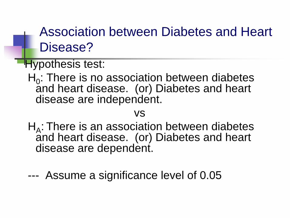
Hypothesis test:
H0: There is no association between diabetes and heart disease. (or) Diabetes and heart disease are independent.
vs
HA: There is an association between diabetes and heart disease. (or) Diabetes and heart disease are dependent.
--- Assume a significance level of 0.05
Association between Diabetes and Heart
Disease?
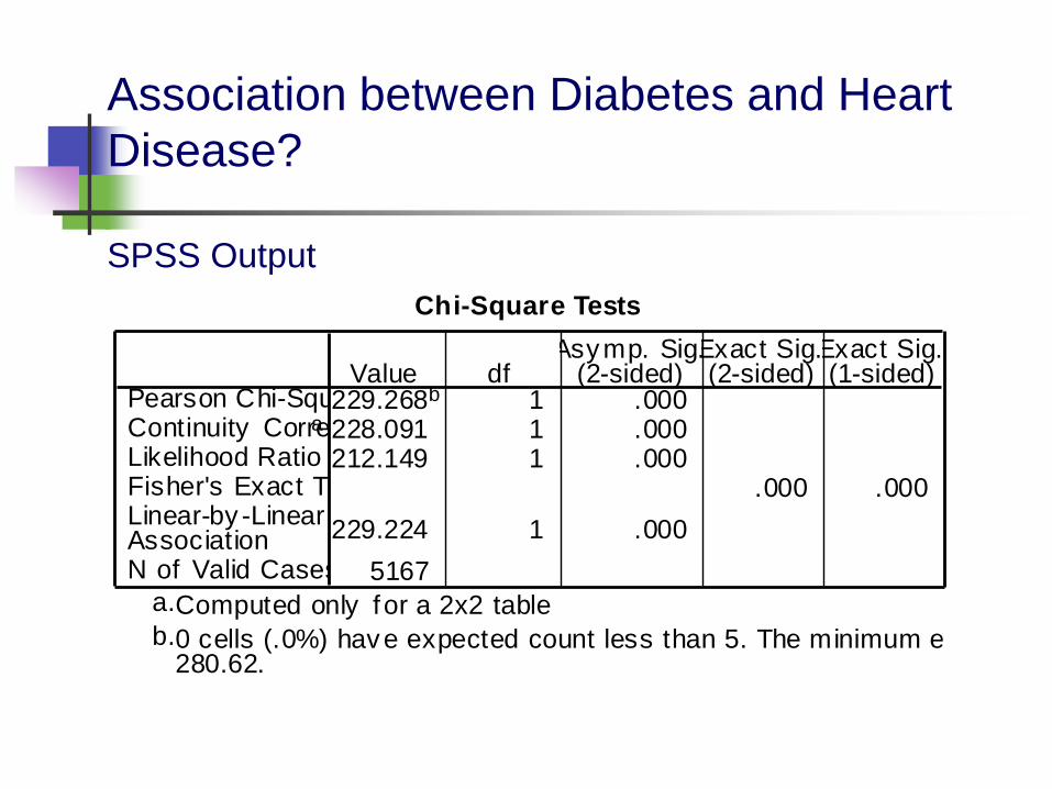
SPSS Output
Chi-Square Tests
229.268b 1 .000228.091 1 .000212.149 1 .000
.000 .000
229.224 1 .000
5167
Pearson Chi-SquareContinuity Correctiona
Likelihood RatioFisher's Exact TestLinear-by -LinearAssociationN of Valid Cases
Value dfAsymp. Sig.
(2-sided)Exact Sig.(2-sided)
Exact Sig.(1-sided)
Computed only for a 2x2 tablea.
0 cells (.0%) have expected count less than 5. The minimum expected count is280.62.
b.
Association between Diabetes and Heart
Disease?
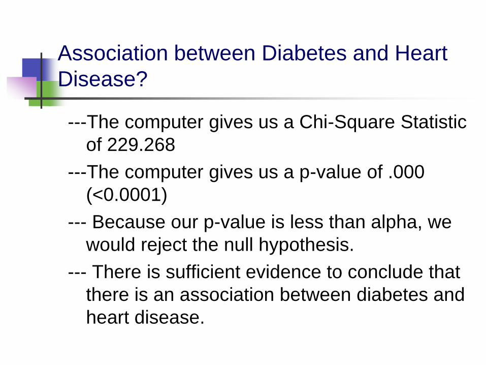
---The computer gives us a Chi-Square Statistic
of 229.268
---The computer gives us a p-value of .000
(<0.0001)
--- Because our p-value is less than alpha, we
would reject the null hypothesis.
--- There is sufficient evidence to conclude that
there is an association between diabetes and
heart disease.
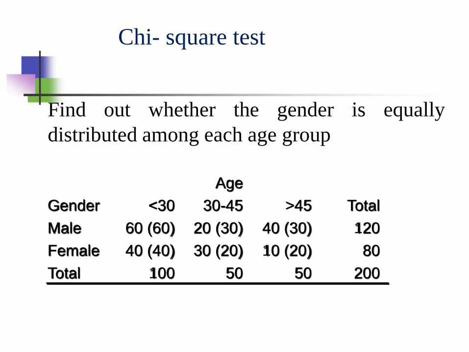
Age
Gender <30 30-45 >45 Total
Male 60 (60) 20 (30) 40 (30) 120
Female 40 (40) 30 (20) 10 (20) 80
Total 100 50 50 200
Chi- square test
Find out whether the gender is equally
distributed among each age group
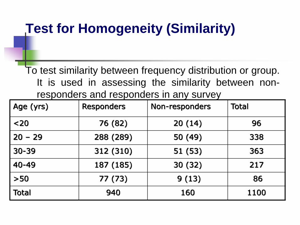
Test for Homogeneity (Similarity)
To test similarity between frequency distribution or group.
It is used in assessing the similarity between non-
responders and responders in any surveyAge (yrs) Responders Non-responders Total
<20 76 (82) 20 (14) 96
20 – 29 288 (289) 50 (49) 338
30-39 312 (310) 51 (53) 363
40-49 187 (185) 30 (32) 217
>50 77 (73) 9 (13) 86
Total 940 160 1100
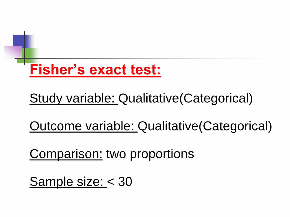
Fisher’s exact test:
Study variable: Qualitative(Categorical)
Outcome variable: Qualitative(Categorical)
Comparison: two proportions
Sample size: < 30
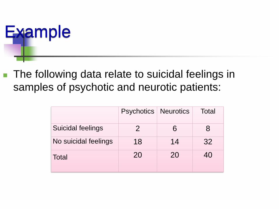
Example
The following data relate to suicidal feelings in
samples of psychotic and neurotic patients:
Psychotics Neurotics Total
Suicidal feelings 2 6 8
No suicidal feelings 18 14 32
Total 20 20 40
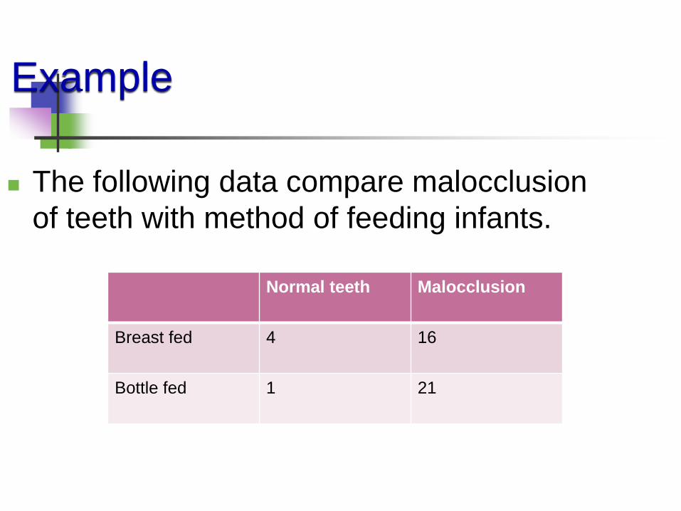
Example
The following data compare malocclusion
of teeth with method of feeding infants.
Normal teeth Malocclusion
Breast fed 4 16
Bottle fed 1 21
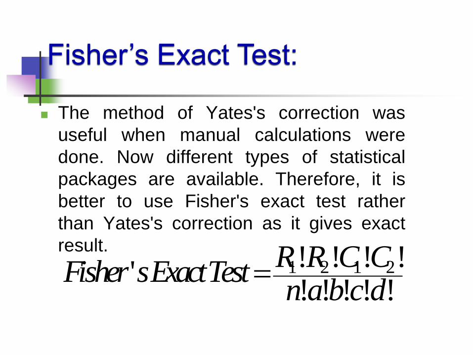
Fisher’s Exact Test:
The method of Yates's correction was
useful when manual calculations were
done. Now different types of statistical
packages are available. Therefore, it is
better to use Fisher's exact test rather
than Yates's correction as it gives exact
result.1 2 1 2! ! ! !
'! ! ! ! !
R R C CFisher sExactTest
n a b c d
What to do when we have a
paired samples and both the
exposure and outcome
variables are qualitative
variables (Binary).
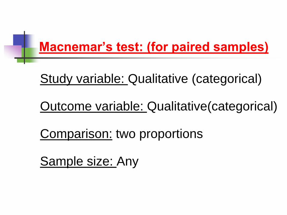
Macnemar’s test: (for paired samples)
Study variable: Qualitative (categorical)
Outcome variable: Qualitative(categorical)
Comparison: two proportions
Sample size: Any
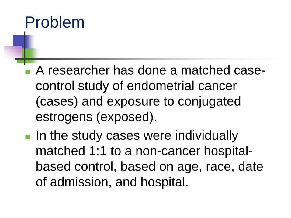
Problem
A researcher has done a matched case-
control study of endometrial cancer
(cases) and exposure to conjugated
estrogens (exposed).
In the study cases were individually
matched 1:1 to a non-cancer hospital-
based control, based on age, race, date
of admission, and hospital.
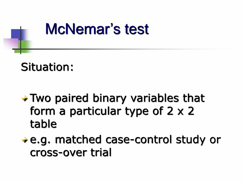
McNemar’s test
Situation:
Two paired binary variables that form a particular type of 2 x 2 table
e.g. matched case-control study or cross-over trial
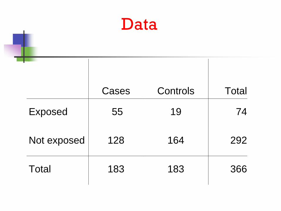
Cases Controls Total
Exposed 55 19 74
Not exposed 128 164 292
Total 183 183 366
Data

can’t use a chi-squared test - observations
are not independent - they’re paired.
we must present the 2 x 2 table differently
each cell should contain a count of the
number of pairs with certain criteria, with
the columns and rows respectively
referring to each of the subjects in the
matched pair
the information in the standard 2 x 2 table
used for unmatched studies is insufficient
because it doesn’t say who is in which pair
- ignoring the matching
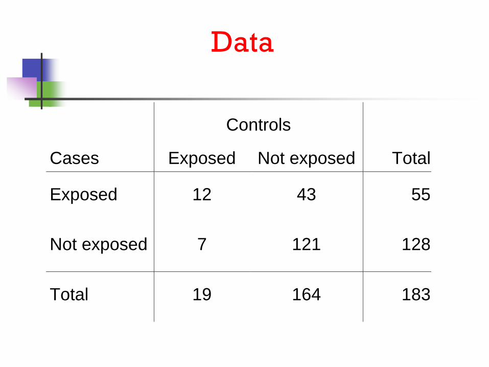
Controls
Cases Exposed Not exposed Total
Exposed 12 43 55
Not exposed 7 121 128
Total 19 164 183
Data
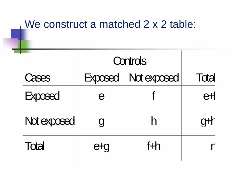
Controls
Cases Exposed Not exposed Total
Exposed e f e+f
Not exposed g h g+h
Total e+g f+h n
We construct a matched 2 x 2 table:
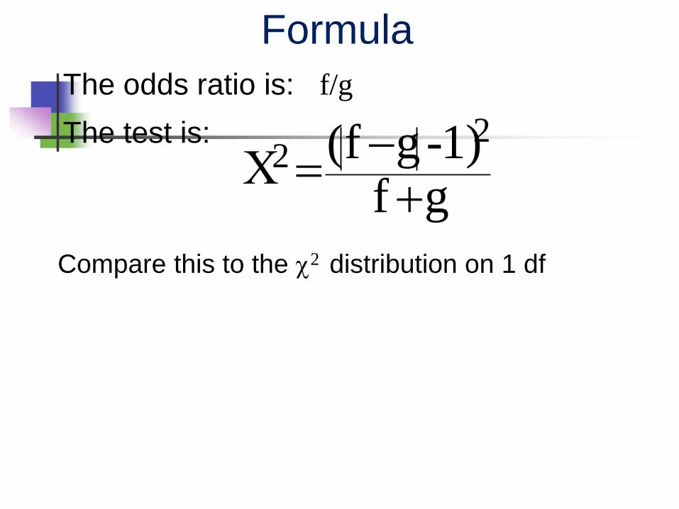
The odds ratio is: f/g
The test is:
Formula
gf1)-gf( 2
2
Compare this to the 2 distribution on 1 df
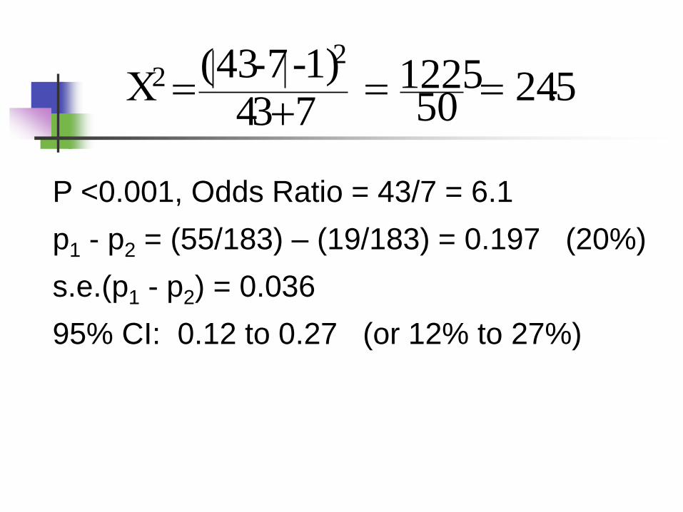
5.2450
12257341)-7-43( 2
2
P <0.001, Odds Ratio = 43/7 = 6.1
p1 - p2 = (55/183) – (19/183) = 0.197 (20%)
s.e.(p1 - p2) = 0.036
95% CI: 0.12 to 0.27 (or 12% to 27%)
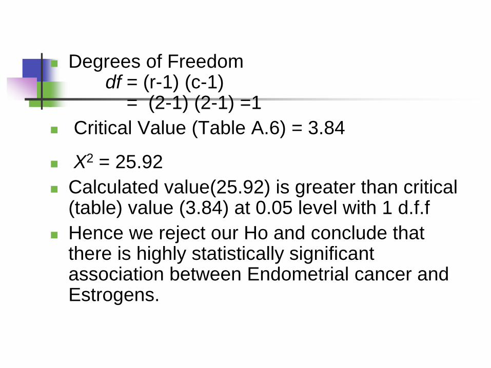
Degrees of Freedomdf = (r-1) (c-1)
= (2-1) (2-1) =1
Critical Value (Table A.6) = 3.84
X2 = 25.92
Calculated value(25.92) is greater than critical (table) value (3.84) at 0.05 level with 1 d.f.f
Hence we reject our Ho and conclude that there is highly statistically significant association between Endometrial cancer and Estrogens.
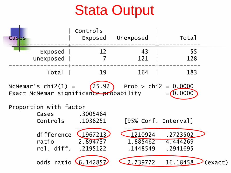
| Controls |Cases | Exposed Unexposed | Total-----------------+------------------------+------------
Exposed | 12 43 | 55Unexposed | 7 121 | 128
-----------------+------------------------+------------Total | 19 164 | 183
McNemar's chi2(1) = 25.92 Prob > chi2 = 0.0000Exact McNemar significance probability = 0.0000
Proportion with factorCases .3005464Controls .1038251 [95% Conf. Interval]
--------- --------------------difference .1967213 .1210924 .2723502ratio 2.894737 1.885462 4.444269rel. diff. .2195122 .1448549 .2941695
odds ratio 6.142857 2.739772 16.18458 (exact)
Stata Output
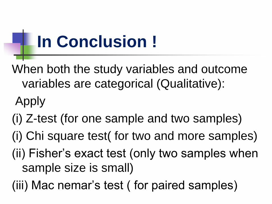
In Conclusion !
When both the study variables and outcome
variables are categorical (Qualitative):
Apply
(i) Z-test (for one sample and two samples)
(i) Chi square test( for two and more samples)
(ii) Fisher’s exact test (only two samples when
sample size is small)
(iii) Mac nemar’s test ( for paired samples)