Statistical Techniques I EXST7005 Start here Measures of Dispersion.

Statistical Techniques I

EXST7005

Start here

Measures of Dispersion

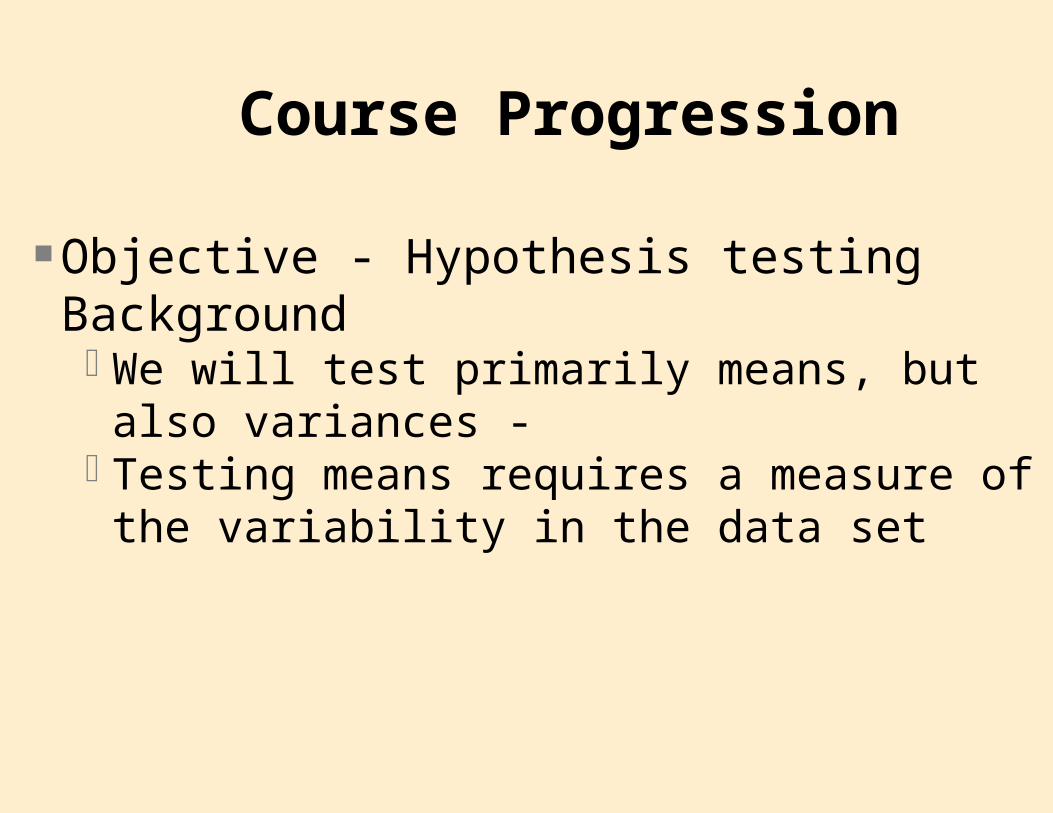
Objective - Hypothesis testing BackgroundWe will test primarily means, but also variances - Testing means requires a measure of the

variability in the data set

Course Progression

MEASURES OF DISPERSION

These are measures of variation or variability among the elements (observations) of a data set

RANGE - difference between the largest and smallest observationThis is a rough estimator which does not use all of

the information in the data set.

MEASURES OF DISPERSION (continued)

Interquartile range - Q1 to Q3 (25% to 75%) better than rangeWhat are Quartiles?

– The first quartile (Q1) is the value that has one quarter of the values below (smaller than Q1) it and three quarters above it (larger than Q1)

– The second quartile has half the values smaller and half the values larger

– The third quartile has 3/4 smaller and 1/4 larger


Percentile - a given percentile has that percent of the values below it and the remaining values above it.

– e.g. The 40th percentile has 40% of the values smaller and 60% of the values larger


VARIANCE the "average" squared deviation from the mean. the POPULATION VARIANCE (called sigma

squared) 2 This is a parameter, and therefore a constantwhere N is the size of the population

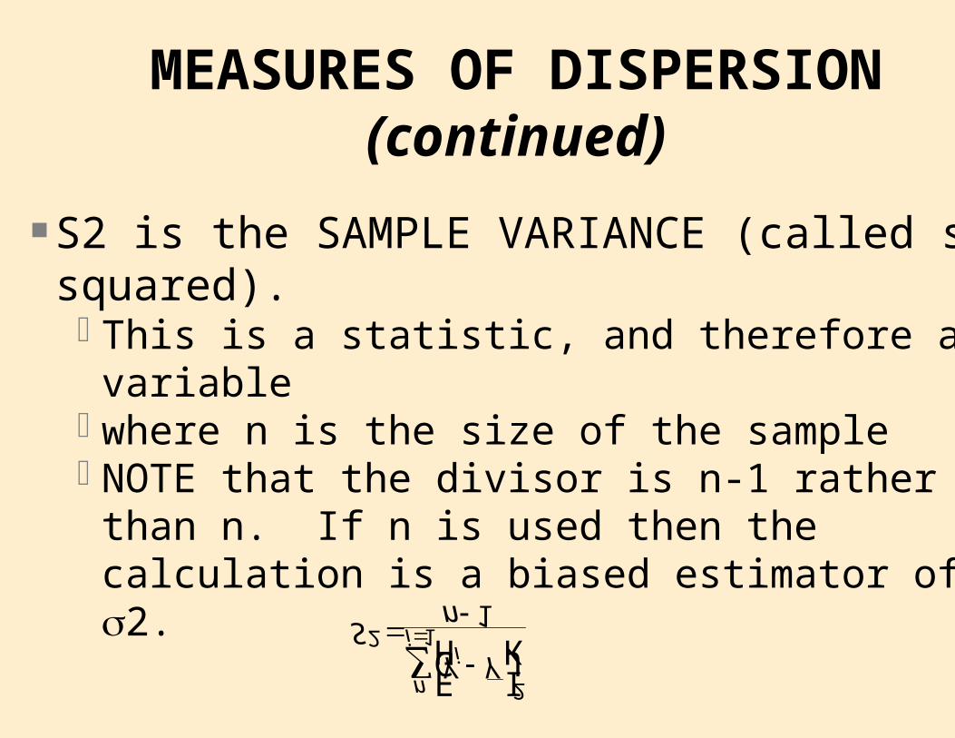
S2 is the SAMPLE VARIANCE (called s-squared).This is a statistic, and therefore a variablewhere n is the size of the sampleNOTE that the divisor is n-1 rather than n. If n is

used then the calculation is a biased estimator of 2.



STANDARD DEVIATION a standard measure of the deviation of observations from the mean. it is calculated as the square root of the variance = 2 this is a parameterS = S2 this is a statistic

the VARIANCE is the average squared deviation, so we take the square root of this to get back to the same units.

Absolute Mean Deviation the "average deviation" from the mean, but using absolute values. This is another possibility, but is not used much because the Variance is more flexible.


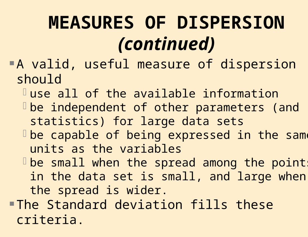
A valid, useful measure of dispersion shoulduse all of the available informationbe independent of other parameters (and

statistics) for large data setsbe capable of being expressed in the same units

as the variablesbe small when the spread among the points in the

data set is small, and large when the spread is wider.

The Standard deviation fills these criteria.


A note on UNITS

When we calculate the mean for a sample or population, the units on the mean are the same as for the original variable. e.g. If the original variable was measured in

inches, the units of the mean will be inches

A note on UNITS (continued)

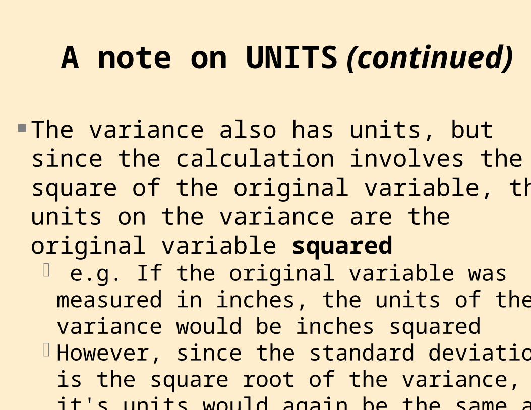
The variance also has units, but since the calculation involves the square of the original variable, the units on the variance are the original variable squared e.g. If the original variable was measured in

inches, the units of the variance would be inches squared

However, since the standard deviation is the square root of the variance, it's units would again be the same as the original variable.

Calculating the Variance The variance can in many cases be calculated more easily with the "calculator formula".

Calculating the Variance (continued)

When we refer to sum of squares or SS, we will refer to the Corrected Sum of Squares, unless otherwise stated. I will generally denote uncorrected sums of squares as UCSS or USS.

The calculator formula is then calculated as

An example of variance

The CORRECTION FACTOR is an adjustment for the MEAN.Examine two samples; Sample 1: 1, 2, 3 Y = 2 Sample 2: 11, 12, 13 Y = 12

Note that the deviations from the mean are the same in each case (-1, 0, 1).

and that SS = (-12)+(0)2+(1)2=2 for both samples

An example of variance (continued)

The SS are Sample 1 SS = 14 - 12 SS = 2 Sample 2 SS = 434 - 432 SS = 2

And the Variance for both samples is then SS / (n-1) = 2 / 2 = 1

So two different looking sets of numbers have the same "scatter" and the same variance.

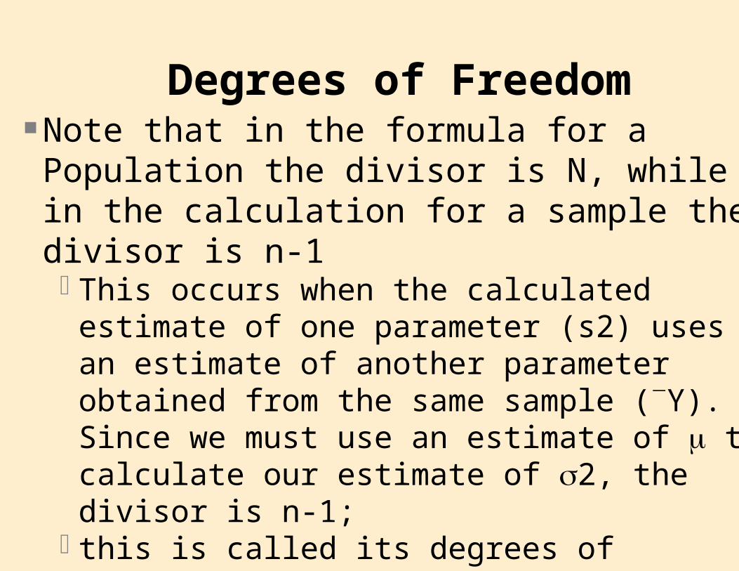
Degrees of Freedom Note that in the formula for a Population the divisor is N, while in the calculation for a sample the divisor is n-1This occurs when the calculated estimate of one

parameter (s2) uses an estimate of another parameter obtained from the same sample (Y). Since we must use an estimate of to calculate our estimate of 2, the divisor is n-1;

this is called its degrees of freedom. If we needed to estimate two parameters prior to being able to estimate a parameter its degrees of freedom would be n-2.

Degrees of Freedom (continued)Why? If we knew , then we could get a deviation

from any single observation.– e.g. If we knew that =5, and we drew an observation

at random and its value was 3, then the deviation would be -2.

However, we cannot get an estimate of 2 from a single sample observation since that observation is also its own mean and the deviation is zero.

– e.g. If we drew a single sample observation, with a value of 3, and we did not know the value of , then we would estimate the value of Y from our sample. That value would also be 3.

Also, with more observations we can have each one deviating independently from , and the sum of the deviations has no restrictions. However, deviations from Y always sum to ZERO, so only the first n-1 can be "any" value, as soon as we know n-1 values, the last one is fixed by our knowledge of Y.

Degrees of Freedom (continued)

COEFFICIENT OF VARIATION CV is the standard deviation expressed as a percent of the mean, e.g. CV = S / Y * 100%

the CV is used to compare relative variation between different experiments or different variables independent of the mean.

EXAMPLES:compare the variability of peoples weights to

peoples heights.compare variation in infants lengths to adult

heights.

COEFFICIENT OF VARIATION (continued)

NUMERICAL EXAMPLE: compare the relative variation in fork length of fish to the weights and scale lengths of the same fish. Data from 3 year old Flier Sunfish (Centrarchus macropterus).

Length (mm)

Weight (g)

Scale Lt. (mm)

Mean 131.8 53.0 6.9Std Dev 15.1 19.6 0.8

COEFFICIENT OF VARIATION (continued)

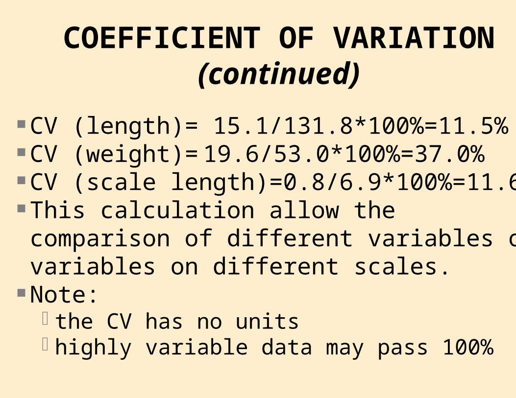
CV (length)= 15.1/131.8*100%=11.5% CV (weight)= 19.6/53.0*100%=37.0% CV (scale length)=0.8/6.9*100%=11.6% This calculation allow the comparison of different variables or variables on different scales.

Note: the CV has no units highly variable data may pass 100%

SAS example (#1 continued) PROC UNIVARIATE DATA=ONE PLOT; VAR SALEPRIC; TITLE3 'Frequency table of house Sale Price'; RUN;

Analysis of house sale price data Table 1.1 from Freund & Wilson, 1997Frequency table of house Sale Price

Univariate Procedure

Variable=SALEPRIC

Moments N 42 Sum Wgts 42 Mean 41.37393 Sum 1737.705 Std Dev 12.44694 Variance 154.9264 Skewness -0.04538 Kurtosis 0.486405 USS 78247.67 CSS 6351.983 CV 30.08403 Std Mean 1.920605 T:Mean=0 21.54213 Pr>|T| 0.0001 Num ^= 0 42 Num > 0 42 M(Sign) 21 Pr>=|M| 0.0001 Sgn Rank 451.5 Pr>=|S| 0.0001

SAS example (#1 continued)

Quantiles(Def=5) 100% Max 75 99% 75 75% Q3 48.9 95% 58.5 50% Med 42.85 90% 55.5 25% Q1 35.5 10% 22 0% Min 15 5% 19 1% 15 Range 60 Q3-Q1 13.4 Mode 37

Extremes Lowest Obs Highest Obs 15( 3) 55.5( 35) 18.9( 4) 56.35( 39) 19( 1) 58.5( 40) 19.8( 2) 61.35( 41) 22( 13) 75( 42)

PROC UNIVARIATE DATA=ONE PLOT; VAR SALEPRIC; TITLE3 'Frequency table of house Sale Price'; RUN;


Stem Leaf # Boxplot 7 5 1 0 7 6 6 1 1 | 5 668 3 | 5 00034 5 | 4 678889 6 +-----+ 4 00334444 8 *--+--* 3 5566777899 10 +-----+ 3 4 1 | 2 66 2 | 2 02 2 | 1 599 3 0 ----+----+----+----+ Multiply Stem.Leaf by 10**+1



Analysis of house sale price data Table 1.1 from Freund & Wilson, 1997Frequency table of house Sale Price

Univariate Procedure

Variable=SALEPRIC

Normal Probability Plot 77.5+ * | +++ | ++++ | +++* | +*+** | +++** 47.5+ ****** | +**** | ***+*** | **++ | ++** | ++++ * 17.5+ *+++* ** +----+----+----+----+----+----+----+----+----+----+ -2 -1 0 +1 +2


EXPECTED VALUES and BIAS

DEFINE Unbiased Estimator: a statistic is said to be an unbiased estimator of a parameter if, with repeated sampling, the average of all sample statistics approaches the parameter.

Expected value: the mean value of a statistic from and infinitely large number of samples (the "long run" average).

EXPECTED VALUES and BIAS (continued)

Note that in dividing by n-1 to calculate variance for a sample, results in a value which is LARGER than if we divide by n. If dividing by n-1 is the correct approach, it suggests that dividing by n causes a negative bias (a value which is, on the average, too SMALL). This is true.

It is true that the expected value of the sample mean is equal to the population parameter. i.e. E{Y} = , and it is also true that E{S2} = 2 , so these are unbiased estimators.

Note that for symmetric distributions, can also be estimated by the median, mode or midrange. However, the MEAN is an unbiased estimator of for all distributions.



Expected Values are actually calculated as the sum (or integration for continuous variables) of the product of the observed values (Yi) in the distribution and the probability of occurrence of each value (p(Yi)). These have various uses, including the evaluation of bias.


For our purposes; The expected value is the measure of the true

central tendency for the probability distribution. If we took all possible samples, the mean of them would be the expected value, provided the estimator we used is unbiased.

For any statistic, if the expected value of the statistic is the same as the population value, the statistic is unbiased.

Summary of Dispersion Dispersion is a measure of the variability among the elements of a population or sample

A number of estimates are available, including Range, Interquartile range, Variance and Standard deviation. All are available from SAS PROC UNIVARIATE.

Units of the variable are squared on variances, but the same as the original variable for standard deviations.

Summary of Dispersion (continued)

Calculations on samples must consider degrees of freedom.

Both the sample mean and sample variance (when divided by "n-1") are unbiased estimators of the population mean and population variance.

Statistical Techniques I EXST7005 Start here Measures of Dispersion.

Documents

Transcript of Statistical Techniques I EXST7005 Start here Measures of Dispersion.