Statistical signal processing methods in scattering - DRS1384/... · Statistical Signal Processing...
140
Statistical Signal Processing Methods in Scattering and Imaging A Dissertation Presented by Maytee Zambrano Núñez to The Department of Electrical and Computer Engineering in partial fulfillment of the requirements for the degree of Doctor of Philosophy in Electrical Engineering Northeastern University Boston, Massachusetts January 2012
Transcript of Statistical signal processing methods in scattering - DRS1384/... · Statistical Signal Processing...

Statistical Signal Processing Methods in Scatteringand Imaging
A Dissertation Presented
by
Maytee Zambrano Núñez
to
The Department of Electrical and Computer Engineering
in partial fulfillment of the requirements
for the degree of
Doctor of Philosophy
in
Electrical Engineering
Northeastern University
Boston, Massachusetts
January 2012

Abstract
This Ph.D. dissertation addresses two related topics in wave-based signal processing:
1) Cramer-Rao bound (CRB) analysis of scattering systems formed by pointlike scatter-
ers in one-dimensional (1D) and three-dimensional (3D) spaces. 2) Compressive optical
coherent imaging, based on the incorporation of sparsity priors in the reconstructions.
The first topic addresses for wave scattering systems in 1D and 3D spaces the infor-
mation content about scattering parameters, in particular, the targets’ positions and
strengths, and derived quantities, that is contained in scattering data corresponding
to reflective, transmissive, and more general sensing modalities. This part of the dis-
sertation derives the Cramer-Rao bound (CRB) for the estimation of parameters of
scalar wave scattering systems formed by point scatterers. The results shed light on
the fundamental difference between the approximate Born approximation model for
weak scatterers and the more general multiple scattering model, and facilitate the iden-
tification of regions in parameter space where multiple scattering facilitates or obstructs
the estimation of parameters from scattering data, as well as of sensing configurations
giving maximal or minimal information about the parameters.
In the 1D case we consider first (in Chapter 1) a number of sensing scenarios and
of a priori data, which simulate different applications in the estimation of parameters
of pointlike scatterers. Later (in Chapter 2) we pay particular attention to elastic scat-
terers, which simplifies the signal model (relative to more general scattering systems),
thereby allowing closed-form expressions for the CRB for special cases. In these chap-
ters the derived CRB results quantify the effect of multiple scattering, be it in enhanc-
ing or in diminishing imaging capabilities, relative to the Born approximation model
i

ABSTRACT ii
which is customarily used as the standard reference for resolution limits (the so-called
“diffraction limit”). The work also discusses the role of the measurement configura-
tion for scatterer information extraction (e.g., reflective data applicable to monostatic
radar, versus transmissive data applicable to bistatic radar). The derived results also
illustrate how specific sensing configurations enhance the estimation associated to the
natural parameters of the system. Finally, the general methods derived for 1D space
are later extended (in Chapter 3) to the 3D case. This includes the adoption in some of
the developments of the fully 3D version of the parameter-reduced model associated to
elastic scattering, but many of the results hold for both elastic and inelastic scatterers.
The derived results are illustrated with numerical examples, with particular emphasis
on the imaging resolution which we quantify via a relative resolution index borrowed
from a previous paper. Additionally, we present details of the estimation performance
for the localization of the targets and the inverse scattering problem.
The second topic of the effort (see Chapter 4) describes a novel compressive-sensing-
based technique for optical imaging with a coherent single-detector system. This hybrid
opto-micro-electromechanical, coherent single-detector imaging system applies the lat-
est developments in the nascent field of compressive sensing to the problem of computa-
tional imaging of wavefield intensity from a small number of projective measurements of
the field. The projective measurements are implemented using spatial light modulators
of the digital micromirror device (DMD) family, followed by a geometrical-optics-based
image casting system to capture the data using a single photodetector. The reconstruc-
tion process is based on the new field of compressive sensing which allows, thanks to
the exploitation of statistical priors such as sparsity, the imaging of the main features
of the objects under illumination with much less data than a typical CCD camera.
The present system expands the scope of single-detector imaging systems based on
compressive sensing from the incoherent light regime, which has been the past focus,
to the coherent light regime which is key in many biomedical and Homeland security

ABSTRACT iii
applications (THz imaging).
The dissertation is organized into an Introduction and 4 Chapters. First we intro-
duce the use of statistical signal processing methods in imaging, with particular focus
on the fundamental Cramer-Rao bound which gives a lower bound for the variance of
any unbiased estimator of the sought-after parameters under a given noise model. The
next two chapters (Chapters 1 and 2) address CRB analysis of scattering systems in 1D
space. The methodology followed in these chapters, and the intuition derived from the
corresponding formulation and computer simulation examples, is the basis of the work
developed in Chapter 3 which considers in detail the CRB analysis of scattering systems
in 3D space. Chapter 4 addresses our theoretical and experimental work toward the
development of a new compressive optical coherent imaging system.


Dedication
This dissertation is lovingly dedicated to my late mother, Brigida Núñez de Zam-
brano. Thanks because all your support, encouragement, and constant love have sus-
tained me throughout my life. I owe every bit of my existence to you. Also I would
like to dedicate this dissertation to my wonderful family. Particularly to my husband,
Ruben whose love and support provided me the strength and perseverance that I needed
to achieve this goal; and to our precious daughters, Maria Celeste and Elizabeth Marie
and our son Ruben Alejandro, who are the joy of our lives.
iv

Acknowledgments
I would like to express my deepest gratitude to my advisor, Dr. Edwin A. Marengo,
for his valuable leadership, support and patience. His enthusiasm and inspiration pro-
vided a constructive guidance, with countless e-mails and worthy discussions. Thanks
Dr. Marengo for always believe in me and most importantly, your friendship during
my graduate studies. Our meetings have enriched my knowledge as well as provided
me with different ways to approach scientific problems. I would also like to thank the
other members of the committee, for their interest in this dissertation.
Special thanks go to SENACYT and Technological University of Panama (UTP)
for their aid that made possible this special long term goal.
I would not have been able to complete this journey without the aid and support
of countless people in Northeastern University such as the staff in CENSSIS and the
Electrical and Computer Engineering department for their assistance and kindness,
especially to Sharon and Joan Pratt.
I expand my thanks to all my CDSP lab mates, whose were sources of laughter, joy,
and support. Special thanks go to Ronald Hernández, Fred Gruber, Laura Dubreuil,
Yueqian Li , Jin He, Parastoo Quarabaqi, and Heidi Sierra. I am very happy that, in
many cases, my friendships with you have extended well beyond our shared time in the
program. I would like to thank them for their valuable comments, insightful discussions
and, specially, their helpful advices on my experience at Northeastern University.
In all of the ups and downs that came my way during the pursuit of my degree, I
thank to my sister Maydee Zambrano, my sister-in-law Matilde Rojas, and my lovely
friend Edith Espino because of your support I was able also to finish this important
v

ACKNOWLEDGMENTS vi
goal. I have been blessed with your presence in my life.
Finally, and most importantly, I would like to thank my husband. His support,
encouragement, patience and unwavering love were undeniably the bedrock upon which
the past years of my life have been built. Especially, his tolerance of my occasional
moods is a testament in itself of his unyielding devotion and love. To my daughter
Maria Celeste whose happiness and love motivated me to keep working even under
adverse situations. I also thank to my late mother Brigida and my father Ricardo, for
their faith in me and allowing me to be as ambitious as I wanted in my life. Thanks
to my Dad and my Aunt Carmen for their words of encouragement and push me for
tenacity and perseverance during this final stage of my dissertation. I have been very
blessed in my life, particularly for all my family love.
Each and everyone listed above and others who have not been named directly, but
whose friendship remains important to me, deserve my gratitude and my admiration
for supporting me throughout this portion of my life and career.

List of Publications
• M. Zambrano N. and E.A. Marengo, "Statistical Study of Multiple Scattering
Effects in the Localization, Resolution, and Inverse Scattering of Two-Point
Scatterer Systems," Journal of the Acoustical Society of America, (to be sub-
mitted).
• Maytee Zambrano-Nunez, Edwin A. Marengo, and David Brady, "Cramer-Rao
study of scattering systems in one-dimensional space", IASTED International
Conference on Antennas, Radar and Wave Propagation, Nov. 1-3, Cambridge,
Massachusetts, 2010.
• Maytee Zambrano-Nunez, Edwin A. Marengo, and Jonathan M. Fisher, "Co-
herent single-detector imaging system", IEEE Workshop on Signal Processing
Systems, San Francisco, California, Oct. 6-8, 2010.
• E.A. Marengo, M. Zambrano-Nunez, and D. Brady, "Cramer-Rao study of
one-dimensional scattering systems: Part I: Formulation", 2009 IASTED In-
ternational Conference on Antennas, Radar, and Wave Propagation, Banff,
Alberta, Canada, July 6-8, 2009.
• E.A. Marengo, M. Zambrano-Nunez, and D. Brady, "Cramer-Rao study of one-
dimensional scattering systems: Part II: Computer simulations", 2009 IASTED
International Conference on Antennas, Radar, and Wave Propagation, Banff,
Alberta, Canada, July 6-8, 2009.
• E.A. Marengo, R.D. Hernandez, Y.R. Citron, F.K. Gruber, M. Zambrano, and
H. Lev-Ari, "Compressive sensing for inverse scattering", XXIX URSI General
Assembly, Chicago, Illinois, Aug. 7-16, 2008.
vii

Introduction
This Ph.D. dissertation is concerned with the formulation of signal processing tech-
niques applied to scattering and imaging systems. Specifically, the first topic of this
Ph.D. dissertation is related to the estimation-theoretic quantification of the “informa-
tion content” about a wave scatterer that is contained in scattered field data. Motivation
is provided by the recent interest on the role of the physical phenomenon of multiple
scattering in either enhancing [1–3] or diminishing [2,3] the imaging capabilities rela-
tive to the classical reference provided by diffraction theory and, in particular, inverse
scattering in the Born approximation, where the well-known “λ/2 limit” applies [4]. It
is important to gain further insight into conditions under which the intrinsic estimation
performance limits associated to the two models exhibit strong disagreement, as well as
the counterpart conditions under which, on the contrary, the mismatch is not significant
whereby the readily tractable Born approximation estimates are good. Our research
builds on recent work, in particular, the investigations carried out by Brancaccio et
al. [5] and Pierri et al. [6], which emphasize the question of the number of degrees of
freedom of the linear mapping from the scattering potential function to the scattering
field data or “essential dimensionality” of the Born-approximated matrix. Our work
uses a different approach based on the fundamental Cramer-Rao bound (CRB) [7],
that addresses both Born-approximable conditions and the more general multiple scat-
tering case, focusing on canonical systems of multiply-scattering point-like scatterers.
In particular, the information about point-like scatterers that is contained in scattering
data is quantified, for different sensing configurations and single- versus multi-frequency
conditions, via the CRB benchmark, which measures under mild statistical conditions
viii

INTRODUCTION ix
the lowest achievable error in the unbiased estimation from noisy scattering data of
sought-after scattering parameters (in the present context, the scattering strengths and
positions of point-like scatterers). It is important to emphasize that the CRB holds for
the given signal model, in other words, the bound on estimation error under multiple
scattering applies to an estimator that uses the correct signal model including multiple
scattering, while the bound for a fictitious or approximate system based on the Born ap-
proximation correspondingly applies to an estimator that uses the Born approximation
model.
To facilitate analytical and computational handling of a variety of interesting ques-
tions, this dissertation considers first the simple case of scatterers or inhomogeneities in
one-dimensional (1D) space. Later we consider the respective generalization in three-
dimensional (3D) space. In both cases we focus on systems formed by only two scatter-
ers. This, on the other hand, is standard in the investigation of the resolution question.
The 1D scenario simulates, e.g., a transmission line environment where the small
scatterer can represent a local inhomogeneity or iris (see figure 1.1(a)), or a canoni-
cal monostatic or bistatic radar or lidar model with “in-line-of-sight” target (see figure
1.1(b)). In the latter context this model is suitable for (transversely) large, (longitu-
dinally) thin planar targets that exhibit negligible variation of constitutive properties
in the transverse coordinates and non-negligible variation mostly in the direction of
propagation of the probing fields, as applicable to far-field transmissive or reflective
tomographic measurements. Extension to the full 3D space involves scattering data
captured for different incident and scattering directions in the 3D space unit sphere
(see figure 3.1). This generalization is key to extend the insight to realistic targets and
systems in 3D space, such as radar and sonar systems for the detection and estimation
of two or more nearby targets.
The use of Cramer-Rao analysis as a tool to assess imaging systems is not new, and
has been a topic of important investigations in the past 40 years. Of much interest is the

INTRODUCTION x
work by Shahram and Milanfar [8] who focused on the rigorous information-theoretic
determination of the resolution of incoherent optical imaging systems by formulating a
detection problem consisting of identifying single-source versus two-source systems and
who also studied the CRB in the estimation of source parameters. However, unlike this
seminal work, which focuses on an incoherent radiation system involving a linear signal
model, we address a coherent scattering system where the signal model is generally
nonlinear. Of greater relevance to the present investigation are a number of more
recent papers by Shi and Nehorai [9], Sentenac et al. [2], Simonetti et al. [1], and
Chen and Zhong [3]. Shi and Nehorai [9] developed a Cramer-Rao analysis of multiply-
scattering point targets in three-dimensional (3D) space and showed via exhaustive
numerical computation that multiple scattering can enhance the estimation and also the
possibility of adding artificial scatterers to enhance estimation of parameters associated
to sought-after scatterers. Simonetti et al. [1] showed that multiple scattering can
significantly enhance imaging while Chen and Zhong [3] showed that there are also
situations where multiple scattering obstructs imaging. Sentenac et al. [2] addressed
the theoretical question of how to define imaging resolution in the nonlinear imaging
regime of multiple scattering, and provided a metric that we adopt later in our own
discussion of resolution in the 3D case. The role of scatterers to enhance imaging has
also been studied in [10], and this issue is, in fact, part of the broader area of radiation
and imaging enhancements via substrate media including metamaterials [11]. Other
studies [12,13] demonstrate enhancements in the diffraction tomography context.
In particular, recently there has been much interest in addressing the resolution
limits in imaging when multiple scattering is significant. This has been investigated
in [1, 2, 9] in connection with the forward point of view, where comparison is made
between two different physical scattering models, one where multiple scattering is neg-
ligible (Born approximation), applicable to weakly scattering objects describable by
the Born approximation, versus the more general one where multiple scattering is sig-

INTRODUCTION xi
nificant and cannot be neglected. This has been investigated also in connection with
the companion inverse point of view or imaging from given data, where one compares
algorithms valid only in the Born approximation versus more general methods appli-
cable in the exact scattering framework [1, 14,15]. It has been shown that so-called
fundamental “resolution limits” in imaging such as the Rayleigh resolution limit hold
only in the Born or linearizing approximation regime, and that they do not generally
hold under active inverse-scattering-based imaging if significant multiple scattering is
involved. Enhancement of resolution via multiple scattering is possible. However, our
work shows clearly that the enhancement may depend on the particular remote sens-
ing configuration and particular scattering parameters, and, in fact, multiple scattering
can either enhance [2,3,9,16] or diminish resolution [2,3,16]. Both possibilities are
clarified further in the present dissertation, in both 1D and 3D spaces.
Unlike previous studies, we provide closed-form solutions for the Fisher informa-
tion and CRB for two-point scatterers, in both 1D and 3D spaces. This allows us to
gain analytical understanding of conditions under which multiple scattering outper-
forms the Born approximation or is detrimental to imaging, and regions in parameter
space and sensing configuration where data yields the largest or smallest information
content. One of the strategies is the reduction of parameter space associated to elastic
scatterers, which we exploit successfully in both 1D and 3D spaces. In addition, we
also address situations where a priori information about the targets may be available,
which simplifies further the analytical results. All the derived results are illustrated
with computer simulations from which we obtain general conclusions about the role of
the scattering parameters and the sensing configuration in the information about scat-
tering parameters that is contained in the scattering data. In addition, throughout the
thesis we follow the theme of constantly comparing the exact multiple scattering results
with the reference Born approximation results. This clarifies the information richness
of the multiple scattering model relative to the linear Born approximation regime. The

INTRODUCTION xii
3D analysis focuses on the radar or sonar scenario, but the results are fundamental and
are also relevant to other areas such as tomography and imaging in general.
It is important to emphasize that the real physical model is, of course, the mul-
tiple scattering one. The Born approximation is valid for weakly scattering objects
only. However, in comparing the two models one gains insight into the possible gain
in resolution due to multiple scattering. Clearly if there are scattering configurations
for which the Born approximation model outperforms the multiple scattering one, this
is clearly a fictitious and non-physically important result, since in the same physical
situation only the multiple scattering model is exact. Thus for fixed scattering param-
eters, if it is found that the CRB using the Born approximation is less than that using
the multiple scattering model, this would mean that the Born-approximation resolution
limit actually is too optimistic for those particular scattering parameters. A completely
different interpretation of the same analysis holds if, on the other hand, one compares
two different systems where the first (multiple scattering) system has given scattering
strengths (say τ1, τ2, · · · ) while the other (Born approximation system) has a scaled
(reduced) value of the same scattering strengths, say τ (B)1 = ατ1, τ
(B)2 = ατ2, · · · where
α ∈ (0, 1) where α is chosen small enough such that the Born approximation holds for
the given positions of the scatterers. In this other interpretation the comparison of mul-
tiple scattering versus Born approximation models is meant to apply to the comparison
of estimation error for target strengths (as a percentage of error relative to the value of
the scattering strength) in strongly scattering versus weakly scattering targets under
the same signal-to-noise ratio (SNR). Clearly both interpretations above are important
in practical application of the results of the present and past CRB studies for scattering
systems.
Our work in CRB for scattering systems also clarifies the role of different mea-
surement configurations for scatterer information extraction. The aspect of sensing
configuration is also treated by Gustafsson and Nordebo [17] who employed the CRB

INTRODUCTION xiii
as a way to assess the ill-posedness of the electromagnetic inverse scattering problem for
nonmagnetic multilayer media(1D), in terms of resolution, as measured by the length
of the grid cells adopted in inversions, versus estimation accuracy, associated to the in-
version of the sought-after constitutive property (permittivity) at each cell. The study
considered time-domain reflective (R) and transmissive (T) data. Some of the results
complement the pioneering work in [17]. For example, among other results, it was
found that transmissive data give a rank-1 Fisher information matrix. But comple-
mentary aspects not addressed in [17] are also considered in chapters 1-2 [16,18,19],
such as the Born approximation versus multiple scattering comparison, more sensing
configurations, in particular, besides R, T, and the one-sided reflective and transmissive
data (RT), we also explore two-sided reflective data plus single-sided transmissive data
(RRT), and two-sided reflective and transmissive data (RRTT)), as well as the role of
a priori information on the scatterer strengths or scatterer positions. In addition, the
parametrization of the system in the case of elastic scattering (see Chapter 2) renders
great simplification which facilitates understanding of the resolution and other ques-
tions. This strategy is also useful for deriving closed-form expressions for the statistical
information associated to each parameter in the system in the 3D case in Chapter 3.
The second topic of this Ph.D. dissertation is related to the reconstruction of the
field intensity images applying the novel technique of compressive sensing. Motivation
is provided by the emerging work of Candès [20] and Donoho [21] which enable the
reconstruction from limited number of random linear projections. Contrarily to the
traditional techniques [22,23], compressive sensing combines the sensing and compres-
sion processes in one step under a known signal sparsity condition. One of the major
breakthroughs in this area has been the invention of the “single-pixel camera” [24,25],
in particular, a camera that uses a single pixel or photodetector to capture the optical
data. This new technology combines 1) compressive sensing algorithms [20, 26, 27],
for the reconstruction of sparse images from limited data, assumed to be in the form

INTRODUCTION xiv
of controllable linear projections of the sought-after object, with 2) the latest spatial
light modulators (digital micromirror devices (DMD)), which are used to create the
projective measurements of the field over the DMD aperture. This approach has been
conclusively demonstrated using incoherent light [24, 25] wherein the relevant signal
model is linear.
This concept has also been extended to the lower frequency terahertz radiation
regime [28] where the signal model is also linear and where, in contrast to the optical
regime (wherein experimental data are “intensity-only”), conveniently both the intensity
and phase of the signals can be measured. The question arises whether this method-
ology can also be implemented with coherent laser light. Optical sensors capture only
field intensity, and this causes the coherent object-to-data mapping to be generally
nonlinear. Clearly it is not obvious whether extension to coherent light of past inco-
herent light and terahertz radiation implementations of single-detector systems based
on compressive sensing is practically feasible. Our work shows that under certain con-
ditions the same general methodology can be extended to coherent laser light where
optical sensors capture only field intensity, and the coherent object-to-data mapping is
generally nonlinear.
Methodologically, chapters 1-3 review the first topic of information content of scat-
tering systems. Specifically, chapter 1 develops the general theory of the CRB for
scattering systems in 1D space, and illustrates the results with many examples. In
chapter 2, we develop further the theoretical CRB expressions by paying particular
attention to elastic scatterers. We generalize those results to the 3D space in Chapter 3
putting particular emphasis on the relation between the CRB and the parameters of the
scattering system as well the effect of the sensing configuration. In these 3 chapters, we
study the impact of the sensing configuration and the scattering parameters in the res-
olution, localization of targets and inverse scattering problem. Additionally, we study
the differences in information content between the Born approximation and the real

INTRODUCTION xv
multiple scattering model. The second topic of compressive-sensing-based technique
for optical imaging is fully developed in chapter 4, including theory and experimental
validation.

Contents
Abstract i
Dedication iv
Acknowledgments v
List of Publications vii
Introduction viii
List of Figures xviii
List of Tables xxiv
Chapter 1. Cramer-Rao Bound Analysis of Scattering Systems in One-dimensional
Space 1
1.1. Scattering Formulation 1
1.2. Scattering Data 3
1.3. Forward Scattering Map in the Born Approximation 5
1.4. Forward Scattering Map Including Multiple Scattering 6
1.5. Cramer-Rao Bound for Two Point Scatterer System in 1D 8
1.6. Fisher Information Matrix 10
1.7. Analysis and Numerical Results 16
1.8. Conclusions 27
Chapter 2. Cramer-Rao Bound Analysis Under Elastic Scattering 30
2.1. Elastic Scattering Condition 30
xvi

CONTENTS xvii
2.2. Fisher Information Matrix 31
2.3. Numerical Illustration 39
2.4. Conclusions 42
Chapter 3. Cramer-Rao Bound Analysis of Scattering Systems in Three-
dimensional Space 47
3.1. The Forward Scattering Mapping 47
3.2. Elastic Scattering Condition in 3D Space 51
3.3. Cramer-Rao Bound Estimation 52
3.4. Numerical Experiments 69
3.5. Conclusions 96
Chapter 4. Compressive Coherent Optical Imaging 100
4.1. Generalities 100
4.2. Compressive Imaging 101
4.3. Optical Signal Model 103
4.4. Results and Discussion 105
4.5. Conclusions 108
Bibliography 111

List of Figures
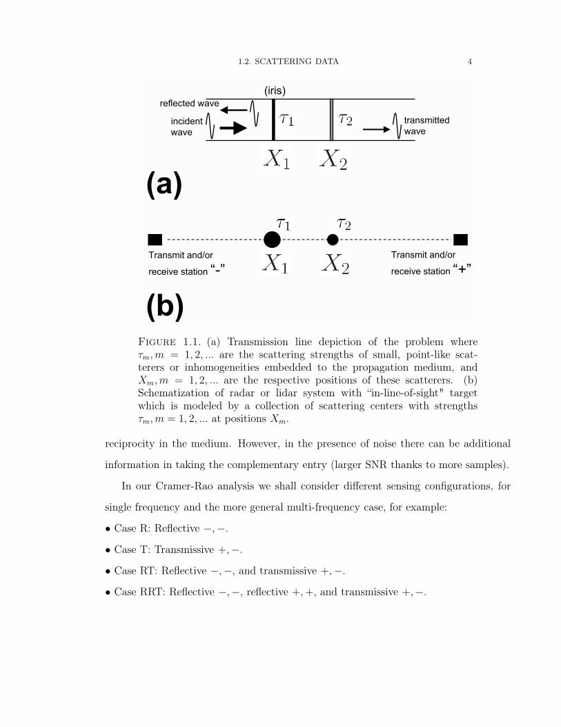
1.1 (a) Transmission line depiction of the problem where τm, m = 1, 2, ...
are the scattering strengths of small, point-like scatterers or inhomo-
geneities embedded to the propagation medium, and Xm, m = 1, 2, ...
are the respective positions of these scatterers. (b) Schematization of
radar or lidar system with “in-line-of-sight" target which is modeled
by a collection of scattering centers with strengths τm, m = 1, 2, ... at
positions Xm. . . . . . . . . . . . . . . . . . . . . . . . . . . . . . . . . . . 4
1.2 CRB(d) for cases RRTT vs noise level for distances d = λ/3, λ/8 for
the no a priori knowledge case. . . . . . . . . . . . . . . . . . . . . . . . . 18
1.3 CRB(τ(r)1) for case RRTT vs noise level for distance d = λ/3, λ/8 for
the no a priori knowledge case. . . . . . . . . . . . . . . . . . . . . . . . . 19
1.4 CRB(d) for case RRTT and RRT vs scatterers’ separation d with σ20 =
10−4 for the no a priori knowledge case. . . . . . . . . . . . . . . . . . . . 20
1.5 CRB((τ(r)1)) for case RRT and RRTT vs scatterers’ separation d with
σ20 = 10−4 for the no a priori knowledge case.. . . . . . . . . . . . . . . . 20
1.6 CRB(d) for cases R, RT, RRT, and RRTT under Born approxima-
tion model vs scatterers’ separation distance d with σ20 = 10−4 for the
“known material” case. . . . . . . . . . . . . . . . . . . . . . . . . . . . . . 21
1.7 CRB(d) for cases R, RT, RRT, and RRTT under multiple scatter-
ing model vs scatterers’ separation distance d with σ20 = 10−4 for the
“known material” case. . . . . . . . . . . . . . . . . . . . . . . . . . . . . . 22
xviii

LIST OF FIGURES xix
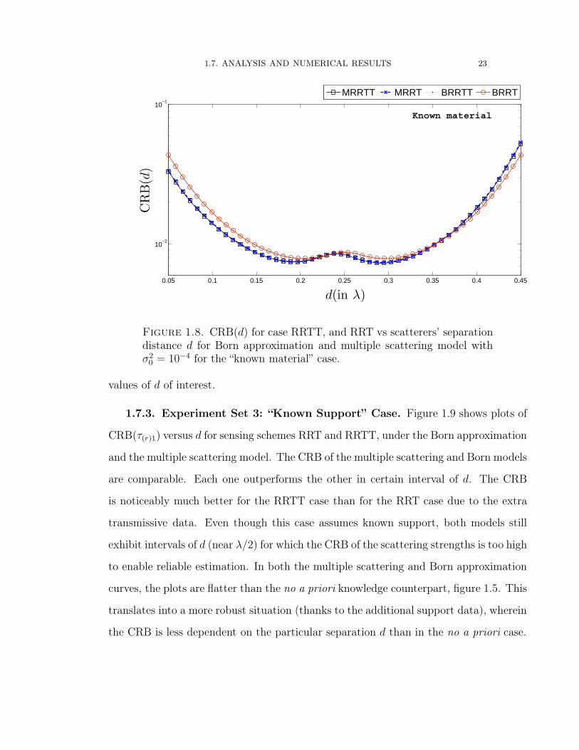
1.8 CRB(d) for case RRTT, and RRT vs scatterers’ separation distance d
for Born approximation and multiple scattering model with σ20 = 10−4
for the “known material” case.. . . . . . . . . . . . . . . . . . . . . . . . . 23
1.9 CRB((τ(r)1)) for case RRTT, and RRT vs scatterers’ separation dis-
tance d for Born approximation and multiple scattering model with
σ20 = 10−4 for the “known support” case. . . . . . . . . . . . . . . . . . . . 24
1.10 CRB(d) per frequency sample for the no a priori knowledge case. σ20 =
10−4. . . . . . . . . . . . . . . . . . . . . . . . . . . . . . . . . . . . . . . . 25
1.11 CRB(τ) per frequency sample for the no a priori knowledge case. σ20 =
10−4. . . . . . . . . . . . . . . . . . . . . . . . . . . . . . . . . . . . . . . . 25
1.12 CRB(τ(r)1) per frequency sample for the “known support” case. σ20 =
10−4. . . . . . . . . . . . . . . . . . . . . . . . . . . . . . . . . . . . . . . . 26
1.13 CRB(d) per frequency sample for the “known material” case. σ20 =
10−4. . . . . . . . . . . . . . . . . . . . . . . . . . . . . . . . . . . . . . . . 27
2.1 CRB(kd) including multiple scattering, versus kd, for σ20 = 10−4, for
data sets R, T, RR, TT, RT, RRT and RRTT. . . . . . . . . . . . . . . . 40
2.2 CRB(�(τ1)/k) including multiple scattering, versus kd, for σ20 = 10−4,
for data sets R, T, RR, TT, RT, RRT, and RRTT. . . . . . . . . . . . . 41
2.3 I(d)MS/I(d)Born for reflective data versus the scattering strengths θm
for m= 1,2, under scatterer separation d = 0.25λ in (top plot) and
d = 0.15λ (bottom plot), with σ20 = 10−4. The top plot corresponds to
R(−,−), while the bottom plot corresponds to R(+,+).. . . . . . . . . . . . 44
2.4 I(d)MS/I(d)Born for reflective data versus θ and d, when both scatterers
have the same reflectivity. The top and bottom plots correspond to the
cases R(−,−) and R(+,+), respectively. . . . . . . . . . . . . . . . . . . . . . 45

LIST OF FIGURES xx
2.5 I(θ1)MS/I(θ1)Born versus θ2 and d. The top left, top right, and bottom
plots correspond to the cases R(−,−), R(+,+) and T , respectively . . . . . 46
3.1 Illustration of a scattering experiment to interrogate two point targets. . 70
3.2 Real and imaginary parts of the target strength under the elastic condition.
70
3.3 CRB(d1) as the observation angle β varies with incident field at α = 0
for the scatterers’ separation d = λ/4 and d = λ/2. . . . . . . . . . . . . 71
3.4 CRB(d1) as the incident angle α varies with observation angle at
β = π − α for the scatterers’ separation d = λ/4 and d = λ/2. Subfig-
ures (a) and (c) correspond to the real multiple scattering model while
subfigures (b) and (d) to the Born approximation model. . . . . . . . . . 73
3.5 CRB(d1) as scatterers’ separation d varies. Plots are generated using
Nr = Nt where α, β ∈ (0, π).. . . . . . . . . . . . . . . . . . . . . . . . . . 74
3.6 Plot of 1/|F|2 with τ1 = τ2 = 1. . . . . . . . . . . . . . . . . . . . . . . . . 74
3.7 CRB(d1) as scatterers’ separation d varies. Plots are generated using
Nr = Nt = 20 evenly spaced in the angular region α, β ∈ (0, θe). . . . . . 76
3.8 CRB(d1) as scatterers’ separation d varies. Plots are generated using
Nr = Nt = 20 evenly spaced in the angular region α ∈ (0, θe) and
β ∈ (π − θe, π). . . . . . . . . . . . . . . . . . . . . . . . . . . . . . . . . . 77
3.9 CRB(d1) as scatterers’ separation d varies. Plots are generated using
Nr = Nt = 20 evenly spaced in the angular region α, β ∈ (π/2 −θB, π/2 + θB). . . . . . . . . . . . . . . . . . . . . . . . . . . . . . . . . . . 77

LIST OF FIGURES xxi
3.10 CRB(d1) as the scatterer strength τ2 increases under the Born ap-
proximation and the multiple scattering model for different targets’
separation d. Plots are generated using a sensing configuration with 10
probing fields and 10 receivers point (α, β ∈ (0, π)) with τ1 = 1. . . . . . 78
3.11 Resolution√CRB(d)/d2 as d increases with τ1 = τ2 = 1 under the
multiple scattering model. . . . . . . . . . . . . . . . . . . . . . . . . . . . 80
3.12 Resolution√CRB(d)/d2 versus d as the number of observations in-
creases with τ1 = τ2 = 1. The observations are collected in the interval
of scattering directions β ∈ [0 − π/4] with α = 0 under the Born
approximation model. . . . . . . . . . . . . . . . . . . . . . . . . . . . . . 81
3.13 Resolution√CRB(d)/d2 versus d as the number of observations in-
creases with τ1 = τ2 = 1. The observations are collected in the interval
of scattering directions β ∈ [0 − π/4] with α = 0 under the multiple
scattering model. . . . . . . . . . . . . . . . . . . . . . . . . . . . . . . . . 82
3.14 Resolution√CRB(d)/d2 versus d with τ1 = τ2 = 1 for different ob-
servation intervals. The plots are generated using 100 observations
collected using a single incident field (α = 0) under both the Born
approximation and the multiple scattering model. . . . . . . . . . . . . . 83
3.15 Resolution√CRB(d)/d2 versus d. Plots are generated using 100 ob-
servations collected using different sensing configurations of 10 probing
field and 10 observations points with α ∈ [0− π/4], β ∈ [3π/4, π]. . . . . 84
3.16 Resolution√CRB(d)/d2 versus d with τ1 = τ2 = 0.0689 + 0.1194i
for different observation intervals. The plots are generated using 100
observations collected using a single incident field (α = 0) under both
the Born approximation and the multiple scattering model. . . . . . . . 85

LIST OF FIGURES xxii
3.17 Resolution√CRB(d)/d2 as τ2 increases with τ1 = 1 for different scat-
terers’ separation d. Plots are generated using 100 observations col-
lected using a 10 probing fields and 10 observation points (α, β ∈ [0, π])
under the Born approximation and the multiple scattering model. . . . . 86
3.18 CRB(Φ) as d varies under the Born approximation and the multiple
scattering models with the elastic strength τ = 0.0689+ 0.1194i . Tra-
jectories are generated using a sensing configurations with 10 probing
fields and 10 receivers point with (a) α, β ∈ [0, π] while subfigure (b)
α ∈ [0, π/4], β ∈ [5π/6, π]. . . . . . . . . . . . . . . . . . . . . . . . . . . . 88
3.19 CRB(τ) as d varies under the Born approximation and the multiple
scattering models for different τ . Trajectories are generated using sens-
ing configurations with 10 probing fields and 10 receivers point with
α ∈ [0, π/4], β ∈ [5π/6, π]. . . . . . . . . . . . . . . . . . . . . . . . . . . . 89
3.20 Log[IMS(ξ)/IB(ξ)] as d and τ increase with real targets strength τ1 =
τ2 = τ . Subfigures (a), (b), and (c) correspond to ξ equal to d, d1, and
τ respectively. . . . . . . . . . . . . . . . . . . . . . . . . . . . . . . . . . . 90
3.21 Log[IMS(ξ)/IB(ξ)] as d and Φ increase with elastic targets strength
τ1 = τ2 = τ = (ei2Φ − 1)/i2k. Subfigures (a), (b), and (c) correspond
to ξ equal to d, d1, and τ respectively. . . . . . . . . . . . . . . . . . . . . 91
3.22 Plot of the magnitude and phase of the scattering amplitude K versus
the angle of reception β with τ1 = τ2 = 1 and α = 0 under the Born
approximation and the multiple scattering model. Subfigures (a) and
(b) correspond to the scatterers’ separation d = 0.08λ while (c) and
(d) to d = 0.5λ. . . . . . . . . . . . . . . . . . . . . . . . . . . . . . . . . . 92

LIST OF FIGURES xxiii
3.23 Plot of the magnitude and phase of the scattering amplitude K as
d varies with τ1 = τ2 = 1 under the Born approximation and the
multiple scattering model. Subfigures (a) and (b) correspond to the
α = π/6, β = 5π/6 while (c) and (d) to α = π/4, β = π/3. . . . . . . . . 94
3.24 Plot of the magnitude and phase of the scattering amplitude K as
τ2 varies with τ1 = 1 under the Born approximation and the multiple
scattering model. Subfigures (a) and (b) correspond to d = 0.01λ while
(c) and (d) to d = 0.02λ.. . . . . . . . . . . . . . . . . . . . . . . . . . . . 95
3.25 Plot of the largest singular value σ1 of K as the scatterers’ separation
d increases for a sensing configuration of 10 probing fields and 10 ob-
servation points (α, β ∈ [0, π]). Subfigures (a) and (b) correspond to
targets strength τ1 = τ2 = 1, while subfigures (c) and (d) to elastic
scatters τ1 = τ2 = 0.0689 + j0.1194. . . . . . . . . . . . . . . . . . . . . . 96
4.1 Optical setup. . . . . . . . . . . . . . . . . . . . . . . . . . . . . . . . . . . 101
4.2 Objects used in the experiments: a) paw print, and c) T. Figures b)
and d) are 300× 300 pixel images of “paw print” and “T”, respectively,
taken with a CCD camera positioned at the DMD plane. . . . . . . . . . 106
4.3 Reconstructions of the “paw print” field. a) 500 mono-patch or semi-
synthetic measurements, b) 409 mono-patch measurements, c) 500 multi-
patch measurements, and d) 350 multi-patch measurements with range
constraints. . . . . . . . . . . . . . . . . . . . . . . . . . . . . . . . . . . . 108
4.4 Reconstructions of the “T” field. a) corresponds to 409 mono-patch or
semi-synthetic samples, b) corresponds to 390 multi-patch data, and c)
corresponds to 204 mono-patch samples.. . . . . . . . . . . . . . . . . . . 109

List of Tables
1.1 Rank of the 7 × 7 Fisher information matrix under single-frequency
(SF) and multi-frequency (MF) conditions for parameter vector ξ =[X1, d, τ(r)1, τ(r)2, τ(i)1, τ(i)2, σ
20
]T . 12
1.2 Rank of the 3 × 3 Fisher information matrix under single-frequency (SF) and
multi-frequency (MF) conditions for parameter vector ξ = [X1, d, σ20]
T . 15
1.3 Rank of the 5 × 5 Fisher information matrix under single-frequency
(SF) and multi-frequency (MF) conditions for parameter vector ξ =[τ(r)1, τ(r)2, τ(i)1, τ(i)2, σ
20
]T . 16
xxiv

CHAPTER 1
Cramer-Rao Bound Analysis of Scattering Systems in
One-dimensional Space
1.1. Scattering Formulation
Consider in 1D free space, primary scalar sources (ρ) and scalar fields (incident
fields) (ψi) related by the scalar Helmholtz equation
(1.1)(∂2
∂x2+ k2
)ψi(x) = ρ(x)
so that the incident fields
(1.2) ψi(x) =
∫G0(x, x
′)ρ(x′)dx′
where the free space Green function (see [29], p. 912)
(1.3) G0(x, x′) = − i
2kexp(ik|x− x′|).
It obeys
(1.4)(∂2
∂x2+ k2
)G0(x, x
′) = δ(x− x′)
and outgoing wave conditions at infinity. In these results, k = ω/c is the wavenumber
of the field at angular oscillation frequency ω where c is the free space speed of light.
1

1.1. SCATTERING FORMULATION 2
For more general media, the differential equation relating sources ρ and (total) fields
ψt is
(1.5)(∂2
∂x2+ k2
)ψt(x) = V (x)ψt(x) + ρ(x)
where V (x) denotes the scattering potential, so that V (x) = κ2(x)− k2. The quantity
κ(x) is the space-dependent wavenumber of the field in the (total) medium.
In this new medium, radiation is governed by
(1.6) ψt(x) =
∫G(x, x′)ρ(x′)dx′
where G is the total Green function in the new medium. It obeys
(1.7)(∂2
∂x2+ k2
)G(x, x′) = V (x)G(x, x′) + δ(x− x′)
To relate this Green’s function to the free space one, we note that Eqs.(1.4,1.7) yield
(after some manipulations involving Green’s theorem)
G(x, x′)−G0(x, x′) =
∫dx′′G0(x, x
′′)V (x′′)G(x′′, x′)(1.8)
=
∫dx′′G(x, x′′)V (x′′)G0(x
′′, x′)
which coincidentally implies from Eqs.(1.2,1.6) the following result valid for rather
general excitations (transmit sources ρ):
(1.9) ψt(x)− ψi(x) =
∫dx′G0(x, x
′)V (x′)ψt(x′) =
∫dx′G(x, x′)V (x′)ψi(x
′).
For the particular case of point-like scatterers of individual strengths or reflectivities
τm, m = 1, 2, ...,M , and positions Xm, m = 1, 2, ...,M , we have V (x) =∑M
m=1 τmδ(x −

1.2. SCATTERING DATA 3
Xm). Then (1.8) gives
G(x, x′)−G0(x, x′) =
M∑m=1
G0(x,Xm)τmG(Xm, x′)(1.10)
=M∑
m=1
G(x,Xm)τmG0(Xm, x′),
a result to be used later, with emphasis on the particular two-scatterer case.
1.2. Scattering Data
In the following it will be assumed that the scatterers are all in the region (0, D),
and that scattering experiments are done involving point sources and receivers at x ≤ 0
and/or x ≥ D.
In this 1D model, the wave scattered field measurements are performed at the
transceivers “-” and “+”, (refer to figure 1.1). It is assumed that transceivers “-” and
“+” are identical and small compared with the wavelength so they are approximated at
point elements at x = 0 and x = D respectively. The scattering data are the outputs
of the different transmit-receive experiments, which can be arranged as the so-called
“multistatic data matrix” or “scattering data matrix” K.
For the purposes of analysis, it will suffice without loss of generality to assume the
following scattering experiments :
• “Reflective”: a point source at x = 0 or x = D (ρ(x) = δ(x − XT )) and a point-
receiver also at x = 0 or x = D. The measured scattered field for this experiment will
be denoted K(−,−) or K(+,+). Those are particular entries in the scattering matrix
K.
• “Transmissive”: a point source at x = 0 or x = D and a point-receiver at x = D or
x = 0 respectively. The entries in the scattering matrix K of these experiments will be
denoted as K(+,−) and K(−,+). These entries are, apart from noise, identical due to
1.2. SCATTERING DATA 4
Figure 1.1. (a) Transmission line depiction of the problem whereτm, m = 1, 2, ... are the scattering strengths of small, point-like scat-terers or inhomogeneities embedded to the propagation medium, andXm, m = 1, 2, ... are the respective positions of these scatterers. (b)Schematization of radar or lidar system with “in-line-of-sight" targetwhich is modeled by a collection of scattering centers with strengthsτm, m = 1, 2, ... at positions Xm.
reciprocity in the medium. However, in the presence of noise there can be additional
information in taking the complementary entry (larger SNR thanks to more samples).
In our Cramer-Rao analysis we shall consider different sensing configurations, for
single frequency and the more general multi-frequency case, for example:
• Case R: Reflective −,−.
• Case T: Transmissive +,−.
• Case RT: Reflective −,−, and transmissive +,−.
• Case RRT: Reflective −,−, reflective +,+, and transmissive +,−.

1.3. FORWARD SCATTERING MAP IN THE BORN APPROXIMATION 5
• Case RRTT: Reflective −,−, reflective +,+, transmissive +,−, and transmissive
−,+.
Each sensing configuration above generates a particular scattering matrix K which
is the key to study the information content through the CRB study. It also allows us
to identify the next optimal experiment in the estimation process.
1.3. Forward Scattering Map in the Born Approximation
The scattered field (total minus incident field) for the above experiments is defined
by G−G0, which according to Eqs.(1.8,1.10) gives:
• K(−,−) = G(0, 0) − G0(0, 0) =∫dx′′G0(0, x
′′)V (x′′)G(x′′, 0) for the case “reflective
−,−”.
• K(+,+) = G(D,D)−G0(D,D) =∫dx′′G0(D, x
′′)V (x′′)G(x′′, D) for the case “reflec-
tive +,+”.
• K(+,−) = G(D, 0) − G0(D, 0) =∫dx′′G0(D, x
′′)V (x′′)G(x′′, 0) = K(−,+) for the
cases “transmissive +,−” or the reciprocal equivalent, case “transmissive −,+”.
Let us emphasize next the particular case of two point-like scatterers of individual
strengths or reflectivities τ1 and τ2 and positions X1 and X2, so that V (x) = τ1δ(x −X1) + τ2δ(x−X2).
In the Born approximation for which G � G0 we then obtain from (1.3,1.10)
(1.11) KB(−,−) =
(− i
2k
)2
exp(i2kX1) [τ1 + τ2 exp(i2kd)]
where it is introduced the target separation d = X2 −X1.
We also obtain
(1.12) KB(+,+) =
(− i
2k
)2
exp[i2k(D −X1 − d)] [τ2 + τ1 exp(i2kd)]

1.4. FORWARD SCATTERING MAP INCLUDING MULTIPLE SCATTERING 6
and
(1.13) KB(+,−) =
(− i
2k
)2
exp(i2kD)(τ1 + τ2) = KB(−,+)
which completes the picture of scattering by two point-like scatterers within the Born
approximation. Let us consider next the more general multiple scattering case.
1.4. Forward Scattering Map Including Multiple Scattering
The more general case of multiply scattering point targets can be readily handled
by carefully following the successive multiple scattering events as is done, e.g., in [30],
p. 220-223 (see, in particular, equations 5.67-d, 5.68 in [30]). (Remark: However, care
must be exercised in noting that the electromagnetic discussion in [30] applies to a
slightly different physical situation, in particular, one of a three-layered medium, unlike
the present medium formed by free space as background and two point-like scatterers
or reflectivities embedded to that background. Thus the results in [30] reduce to the
results presented in this work after certain substitutions: in this case, scattering by
the point-like inhomogeneities is isotropic, hence the reflectivity by coming from the
right is the same as by coming from the left, unlike in the layered medium where the
reflectivity varies in sign when applied to the opposite direction of travel. But besides
this issue, the results in [30] and the present results outlined below are equivalent.)
One obtains the multiple scattering generalization of (1.11)
(1.14) K(−,−) =
(− i
2k
)exp(i2kX1)
[τ1 +
(1 + τ1)2τ2 exp(i2kd)
1− τ1τ2 exp(i2kd)
]where the expression of τm have introduced for notational compactness
(1.15) τm =
(− i
2k
)τm m = 1, 2.

1.4. FORWARD SCATTERING MAP INCLUDING MULTIPLE SCATTERING 7
Similarly, the multiple scattering generalization of (1.12) is found to be
(1.16) K(+,+) =
(− i
2k
)exp[i2k(D −X1 − d)]
[τ2 +
(1 + τ2)2τ1 exp(i2kd)
1− τ1τ2 exp(i2kd)
].
Finally, the multiple scattering generalization of (1.13) is
(1.17) K(+,−) =
(− i
2k
)exp(i2kD)
[(1 + τ1)(1 + τ2)
1− τ1τ2 exp(i2kd)− 1
]= K(−,+).
1.4.1. Born versus Multiple Scattering Analysis in One-dimensional Space.
Some differences become obvious in terms of the information available in the multiple
scattering case, due to greater contrast giving rise to multiple scattering, versus in
the Born approximation case for weakly scattering targets. For example, the Born
approximation scattering matrix entry KB(+,−) in (1.13) has no dependence on the
target separation d, while the multiple scattering counterpart (1.17) does exhibit such
a dependence. Thus in the Born approximation the transmissive experiment giving
KB(+,−) provides no information about the target separation, but instead gives only
(apart from a constant) the sum of the two target strengths (corresponding to low-
frequency information about the scattering potential as a whole). In contrast, in the
more general multiply scattering case the same transmissive experiment does provide
such information thanks to multiple scattering events between the two scatterers.
Note, however, that the dependence on d is of the form exp(i2kd) which implies
that d and d + nλ/2, n = 1, 2, ... (where λ = 2π/k) exhibit the same value of K(+,−)
so that even in the multiple scattering case show limitations in resolution ability under
a single frequency experiment (we cannot distinguish between distances separated by
half wavelength). (Remark: This problem does not hold in the 2D or 3D case since
then there is wave amplitude attenuation in propagation, which is not present in the 1D
case). However, this is an aliasing issue, and it does not mean that the subwavelength
scatterer separations can not be estimated. As we will show next, we can, in the multiple

1.5. CRAMER-RAO BOUND FOR TWO POINT SCATTERER SYSTEM IN 1D 8
scattering signal model. But, subject to the ambiguity whether the estimated distance
is, say, d, or d+nλ/2, n = 1, 2, .... It is in the latter interpretation that we will speak in
the following about subwavelength imaging resolution. (with the clear understanding
that we are referring to estimation of the “principal value”of d only).
Our next goal is to quantify and better understand the information content for a two-
scatterer system characterized by scattering strengths τ1 and τ2, and scatterer position
X1 and target separation d, from different scattering data sets. This will be done
via the fundamental Cramer-Rao bound pertinent to the variance (error) of unbiased
estimators for the scattering parameters τ1, τ2, d and X1, under the two signal models
above (Born versus multiple scattering), under different configurations (data sets R, T,
RT, RRT, RRTT), and for single- versus multi-frequency data.
1.5. Cramer-Rao Bound for Two Point Scatterer System in 1D
The Cramer-Rao study is developed directly in the multi-frequency case under the
assumption that the scattering strengths are frequency-independent (nondispersive me-
dia) for the frequency bands used in the interrogation experiments, thus in the multi-
frequency case we consider τm(ω) = τm, m = 1, 2. This assumption simplifies the
analysis and applies to many practical situations.
1.5.1. Signal Model Parameters. In practice, one collects noisy data which we
take into account via the signal model:
(1.18) K (ξ) = K (ξ) +W
where K (ξ) is the noise-free data vector formed by the available entries of the response
matrix K, which depend on the remote sensing configuration (R, T, RT, etc.), K(ξ) is
the noisy realization of that matrix, W is white Gaussian noise with variance σ20 (which
is handled next as nuisance parameter that needs to be estimated from the data), and ξ

1.5. CRAMER-RAO BOUND FOR TWO POINT SCATTERER SYSTEM IN 1D 9
is the vector of the scattering plus noise parameters that ones wishes to estimate from
the data. We consider different vectors ξ corresponding to different combinations of the
following parameters: The position X1 of target 1, the target separation d, the real and
imaginary parts τ(r)m and τ(i)m of target strength τm, m = 1, 2, and the unknown noise
variance σ20. Thus we consider the case of no a priori knowledge, where the parameter
vector
(1.19) ξ =[X1, d, τ(r)1, τ(r)2, τ(i)1, τ(i)2, σ
20
]T(where T denotes transpose) as well as the special cases where τ1, τ2 are known (mod-
eling a priori knowledge of the scatterer’s materials or “Known material case”), so that
(1.20) ξ =[X1, d, σ
20
]Tand where the positions X1, X2 (and thus also d) are known (modeling a priori knowl-
edge of the support of the scatterers or “ Known support case”), so that
(1.21) ξ = [τ(r)1, τ(r)2, τ(i)1, τ(i)2, σ20]
T .
In the following we shall refer to the cases in (1.20) and (1.21) as “known material” and
“known support”, respectively. The three cases in (1.19, 1.20, 1.21) can be considered
under single- and multi-frequency data.
Consider first the single-frequency case. Then for the different remote sensing cases,
the noise-free data vector K is as follows (with T denoting transpose):
• Case R: K = [K(−,−)]
• Case T: K = [K(+,−)]
• Case RT: K = [K(−,−) K(+,−)]T
• Case RRT: K = [K(−,−) K(+,−) K(+,+)]T
• Case RRTT: K = [K(−,−) K(+,−) K(−,+) K(+,+)]T
1.6. FISHER INFORMATION MATRIX 10
If data are gathered for a number Nf of frequencies ω1, ..., ωNf, then in place of the
scalar K(−,−) we have the vector [K(−,−;ω1) ... K(−,−;ωNf)]T , and so on. Then
the noise-free data vector for each case is as follows:
• Case R: K = KT−,−,Nf
≡ [K(−,−;ω1) ... K(−,−;ωNf]T
• Case T: K = KT+,−,Nf
≡ [K(+,−;ω1) ... K(+,−;ωNf]T
• Case RT: K = [K−,−,NfK+,−,Nf
]T
• Case RRT: K = [K−,−,NfK+,−,Nf
K+,+,Nf]T (where K+,+,Nf
is the “+,+”
analog of the “-,-” quantity K−,−,Nfdefined above).
• Case RRTT: K = [K−,−,NfK+,−,Nf
K−,+,NfK+,+,Nf
]T
1.6. Fisher Information Matrix
The corresponding Fisher information matrix I(ξ) is given by [7, eq.15.52]
(1.22) I(ξ)i,j= tr
[C−1
˜K(ξ)
∂C˜K(ξ)
∂ξiC−1
˜K(ξ)
∂C˜K(ξ)
∂ξj
]+2�
[∂KH(ξ)
∂ξiC−1
˜K(ξ)
∂K(ξ)
∂ξj
]
where H denotes the conjugate transpose, and C˜K denotes the covariance matrix [7,
pp. 501] which in our case is simply C˜K = σ2
0I. Here I denotes the identity matrix,
whose size is determined by the length of the data vector K which we will denote next as
L. The CRB (CRB[ξ(i)]) is the lower bound for the variance var[ξ(i)] of any unbiased
estimator for the parameter ξ(i), and is defined in terms of the Fisher information
matrix I(ξ) by [7, eq.3.20]
(1.23) var[ξ(i)] ≥ [I−1(ξ)]i,i = CRB[ξ(i)].
which is achievable under mild conditions ( [31, Chapter 3], [32, p. 169-171]).
Under the parameter vector ξ in (1.19) which is of length 7, the Fisher information
matrix associated to the signal model Eq.(1.18) reduces (for both Born and multiple
1.6. FISHER INFORMATION MATRIX 11
scattering cases) to
I (ξ) =
[L
σ40
δi,jδi,7
]+
2
σ20
�[∂KH (ξ)
∂ξi
∂K (ξ)
∂ξj
]
=
[L
σ40
δi,jδi,7
]+
2
σ20
�
⎡⎢⎢⎢⎢⎢⎢⎢⎣
∂ ˜KH
∂X1
∂ ˜K∂X1
. . . ∂ ˜KH
∂τ(i)2
∂ ˜K∂X1
0
... . . . ......
∂ ˜KH
∂X1
∂ ˜K∂τ(i)2
. . . ∂ ˜KH
∂τ(i)2
∂ ˜K∂τ(i)2
...
0 . . . . . . 0
⎤⎥⎥⎥⎥⎥⎥⎥⎦(1.24)
The results for the parameter vectors ξ in (1.20) and (1.21) are of the same general
form, and are constructed by suitable reduction of the Fisher information matrix above,
thus, for example, for the ξ vector in (1.20) (“known material” case) one obtains
I (ξ) =
[L
σ40
δi,jδi,3
]+
2
σ20
�
⎡⎢⎢⎢⎣∂ ˜KH
∂X1
∂ ˜K∂X1
∂ ˜KH
∂d∂ ˜K∂X1
0
∂ ˜KH
∂X1
∂ ˜K∂d
∂ ˜KH
∂d∂ ˜K∂d
0
0 0 0
⎤⎥⎥⎥⎦(1.25)
Let us highlight salient aspects of each case (R, T, RT, etc., and Born versus multiple
scattering) separately. Rather than providing the analytical expressions for the Fisher
information matrix for each case, which would account for a lengthy discussion, we limit
to highlighting the general structure and rank of this matrix for each case. Tables of the
rank of the Fisher information matrix for representative cases of interest are provided in
Tables 1, 2, and 3, for the parameter vectors in Eq.(1.19), (1.20) and (1.21), respectively.
• Case R: In this case K = K(−,−) + W , where in general K(−,−) is given by
(1.14) while in the Born approximation it is approximated by KB(−,−) in (1.11).
Consider the single frequency case Nf = 1. In this case the Fisher information matrix
has at most rank 3 so that in the no a priori knowledge and “known support” cases
the Fisher information matrix is singular and it is not possible to estimate all the
desired parameters from the data. However, the “known material” case which has only

1.6. FISHER INFORMATION MATRIX 12
Table 1.1. Rank of the 7 × 7 Fisher information matrix under single-frequency (SF) and multi-frequency (MF) conditions for parameter vectorξ =
[X1, d, τ(r)1, τ(r)2, τ(i)1, τ(i)2, σ
20
]T .
Cases τ1=−0.5+i0.5 τ1=−0.5+i0.5 τ1=−0.5+i0.5 τ1=−0.5+i0.5τ2=−0.5+i0.5 τ2=−0.9+i0.3 τ2=−0.9+i0.3 τ2=−0.9+i0.3
SF SF MF(2 freq.) MF (3 or more freq.)BR 3 3 5 7MR 3 3 5 7BT 3 3 3 3MT 3 3 6 6BRT 5 5 7 7MRT 5 5 7 7BRRT 6 7 7 7MRRT 6 7 7 7BRRTT 6 7 7 7MRRTT 6 7 7 7
3 unknown parameters admits a non-singular Fisher information matrix, so that the
CRB can be studied in that case. The rank is 3 since the signal is complex-valued
so that K(−,−) contains two independent data points and the noise is independent
from the signal which gives up to 2 scattering system features plus 1 noise feature (σ20)
that can be estimated from the data, hence the rank 3. In the multi-frequency case
this reflective configuration achieves a full-rank, invertible Fisher information matrix
(meaning that all parameters can be estimated with finite error) with at least 3 different
data frequencies for the no a priori knowledge case and 2 different frequencies for the
“known support” case. The rank remains 3 even for multiple frequencies in the “known
material” case. This was validated with several numerical examples during the course
of this investigation (refer to Tables 1, 2, and 3).
• Case T: Consider first the single-frequency regime, in the Born approximation. From
(1.13), clearly the signal does not depend on X1 or d, i.e., ∂ ˜K∂X1
= 0 = ∂ ˜K∂d
, so that the

1.6. FISHER INFORMATION MATRIX 13
general expression (1.24) takes the following reduced form
(1.26) I [(ξ)]=
[1
σ40δi,jδi,7
]+
2
σ20
�
⎡⎢⎢⎢⎢⎢⎢⎢⎢⎢⎢⎢⎢⎢⎣
0 . . . . . . . . . . . . 0
0 . . . . . . . . . . . . 0
0 0 ∂ ˜KH
∂τ(r)1
∂ ˜K∂τ(r)1
. . . ∂ ˜KH
∂τ(i)2
∂ ˜K∂τ(r)1
0
......
... . . . ......
...... ∂ ˜KH
∂τ(r)1
∂ ˜K∂τ(i)2
. . . ∂ ˜KH
∂τ(i)2
∂ ˜K∂τ(i)2
...
0 . . . . . . . . . . . . 0
⎤⎥⎥⎥⎥⎥⎥⎥⎥⎥⎥⎥⎥⎥⎦which means that, as outlined earlier, there is no information in the data about the
target positions. As illustrated in Tables 1 and 3, the rank is 3 in the no a priori
knowledge and “known support” cases. But in the “known material” case the rank is 1.
These results hold for both single and multiple frequencies. The rank 1 is associated only
to the noise since there is no information in the T data about the target positions. The
information content associated to the transmissive experiment is only on the scattering
strengths, and we will see that transmissive data in combination with reflective data
(e.g., in the RRT and RRTT cases to be studied in further detail next) does enhance
the estimation performance pertinent to the scattering strengths.
In the more general multiple scattering regime addressed in (1.17) the data still
does not depend on X1 (hence ∂K(+,−)∂X1
= 0) but unlike the Born approximation the
data now depends on the target separation d, so that (in contrast with (1.26)) the
Fisher information has the more general structure
(1.27) I [(ξ)] =
[Nf
σ40
δi,jδi,7
]+
2
σ20
�
⎡⎢⎢⎢⎢⎢⎢⎢⎢⎢⎢⎣
0 . . . . . . . . . 0
... ∂ ˜KH
∂d∂ ˜K∂d
. . . ∂ ˜KH
∂τ(i)2
∂ ˜K∂d
......
... . . . ......
... ∂ ˜KH
∂d∂ ˜K
∂τ(i)2. . . ∂ ˜KH
∂τ(i)2
∂ ˜K∂τ(i)2
...
0 . . . . . . . . . 0
⎤⎥⎥⎥⎥⎥⎥⎥⎥⎥⎥⎦

1.6. FISHER INFORMATION MATRIX 14
In this case the rank is 3 in the no a priori knowledge and “known support” cases, and
it is 2 in the “known material” case for a single frequency. The latter is an enhancement
due to multiple scattering, relative to the Born model where the rank is only 1.
Note that for the three situations associated to the parameter vector ξ, the Fisher
information matrix is singular under the transmissive data set alone, for a single fre-
quency. In the multi-frequency case, the rank is at most 6 for the no a priori knowledge
case and remains 2 in the “known material” case. However, in the “known support” case
the rank is 5 (full rank), consequently finite CRB for the five parameters (strengths and
noise) can be computed in this case.
• Case RT: The Fisher information matrix for this case has the general form Eq.(1.24)
with L = 2Nf . In the single-frequency regime, under the Born approximation, ∂ ˜K∂d
=[∂KB(−,−)
∂d0]T
and a similar expression for X1. Under multiple scattering, there is
greater dependence on d but ∂ ˜K∂X1
=[∂K(−,−)
∂X10]T
.
In this case the rank of the Fisher information matrix is 5 in the no a priori knowl-
edge and “known support” cases, and 3 for the “known material” case for single frequency
case. Therefore in the case RT, and under the “known material” and “known support”
cases the Fisher information matrix is invertible (hence all the parameters can be esti-
mated with finite error). In the multi-frequency case the rank of the Fisher information
matrix increases for the no a priori knowledge case, and the Fisher information matrix
becomes invertible for at least two different data frequencies.
• Case RRT: The Fisher information matrix has the general form Eq.(1.24) with
L = 3Nf . In the single-frequency regime, under the Born approximation, ∂ ˜K∂d
=[∂KB(−,−)
∂d0 ∂KB(+,+)
∂d
]Tand a similar expression for X1. In the multiple scattering
model there is greater dependence on d but ∂ ˜K∂X1
=[∂KB(−,−)
∂X10 ∂KB(+,+)
∂X1
]T.
The rank for the no a priori knowledge case is now at most 7, and this value is
achieved if τ1 �= τ2. However for τ1 = τ2 the rank was found to be 6 in the single

1.6. FISHER INFORMATION MATRIX 15
Table 1.2. Rank of the 3 × 3 Fisher information matrix under single-frequency (SF) and multi-frequency (MF) conditions for parameter vectorξ = [X1, d, σ
20]
T .
Cases τ1=−0.5+i0.5 τ1=−0.5+i0.5 τ1=−0.5+i0.5 τ1=−0.5+i0.5τ2=−0.5+i0.5 τ2=−0.9+i0.3 τ2=−0.5+i0.5 τ2=−0.9+i0.3
SF SF MF MFBR 3 3 3 3MR 3 3 3 3BT 1 1 1 1MT 2 2 2 2BRT 3 3 3 3MRT 3 3 3 3BRRT 3 3 3 3MRRT 3 3 3 3BRRTT 3 3 3 3MRRTT 3 3 3 3
frequency case (refer to Table 1). But for multiple frequency one recovers the rank 7.
For the “known material” and “known support” cases the Fisher information matrix
is full rank, as is illustrated in Tables 2 and 3, hence all parameters can be estimated
with finite error. These results hold, for both single and multiple frequency conditions,
and for both Born and multiple scattering models.
• Case RRTT: Since the signalsK(+,−) andK(−,+) are identical, one expects that the
additional data entry will provide only marginal extra information about the scattering
parameters relative to case RRT. This will be illustrated in the computer simulations
section. In this case the Fisher information matrix is of the general form Eq.(1.24) with
L = 4Nf and, in the Born approximation model ∂ ˜K∂d
=[
∂KB(−,−)∂d
0 0 ∂KB(+,+)∂d
]Tand a similar expression for X1. In the multiple scattering model, there is greater
dependence on d, and ∂ ˜K∂X1
=[
∂KB(−,−)∂X1
0 0 ∂KB(+,+)∂X1
]T. The Fisher information
matrix is full rank in this case (see Tables 1, 2, and 3), except in the single frequency
case when τ1 = τ2.

1.7. ANALYSIS AND NUMERICAL RESULTS 16
Table 1.3. Rank of the 5 × 5 Fisher information matrix under single-frequency (SF) and multi-frequency (MF) conditions for parameter vectorξ =
[τ(r)1, τ(r)2, τ(i)1, τ(i)2, σ
20
]T .
Cases τ1=−0.5+i0.5 τ1=−0.5+i0.5 τ1=−0.5+i0.5 τ1=−0.5+i0.5τ2=−0.5+i0.5 τ2=−0.9+i0.3 τ2=−0.5+i0.5 τ2=−0.9+i0.3
SF SF MF MFBR 3 3 5 5MR 3 3 5 5BT 3 3 3 3MT 3 3 5 5BRT 5 5 5 5MRT 5 5 5 5BRRT 5 5 5 5MRRT 5 5 5 5BRRTT 5 5 5 5MRRTT 5 5 5 5
1.7. Analysis and Numerical Results
In this Section several CRB results are presented and discussed that are pertinent
for both the Born approximation signal model, and the more general multiple scatter-
ing signal model. We consider scatterers separation d in the interval (0, λ/2) where the
wavelength λ = 2π/k which entails the aliasing issue addressed earlier, by which in the
1D case it is not possible to differentiate between distances d and d+nλ/2, n = 1, 2, ....
Thus in the following we shall focus on distances d ∈ (0, λ/2), in the motivational con-
text of the question of subwavelength resolution in the 1D case, and related questions.
In the multi-frequency case, the condition becomes d ∈ (0, λmax/2) where λmax is the
largest wavelength used for probing. As particular values of the scattering strengths,
we adopt for the illustrations τ1 = −0.5 + i0.5 and τ2 = −0.9 + i0.3, which obey the
elastic scattering condition presented in detail in Section 2.11
1Remark: As explained earlier, in employing the Born approximation for these values, one of the twointerpretations is that the associated results hold for reduced scattering strengths ατ1 and ατ2 whereα << 1. However, the respective small scattering strengths do not obey the elastic scattering conditionin Section 2.1.

1.7. ANALYSIS AND NUMERICAL RESULTS 17
The computer results are organized into experiment sets 1, 2 and 3, corresponding to
the no a priori knowledge, “known material”, and “known support” cases, respectively.
Within each experiment, the results are elaborated for the two physical models of
interest (Born approximation versus multiple scattering), and provide the associated
comparative analysis. Particular attention is given to the CRB dependence on noise
level, and on scatterer separation d. Another question of much interest which drives
some of our discussion is the comparison of information-extraction capabilities per data
sample (or in communication language, per use of the remote sensing system), associated
to different sensing modalities (R, T, RT, etc.), to different frequencies, to different
target geometries, etc. Thus, we wonder: What is the optimal “next measurement”,
giving the largest information about the parameters of interest? The next measurement
is characterized by the modality or modes used for sensing, which can be the spatial or
geometrical sensing modality R, T, RT, and so on, and/or combinations of spatial and
temporal modes as characterized by the spatial sensing modality and the companion
frequency used in the interrogation. In the single frequency case of this section, clearly
attention is restricted to the spatial issues. But the following section addresses the full
space-frequency modes.
1.7.1. Experiment Set 1: No a priori Knowledge Case. In this experiment,
the wavenumber is considered k = 2π/λ, for unit-value lambda λ = 1. Particular
attention is given to the CRB for estimation of d and τ1, for different values of noise
level (σ20) and d. As explained earlier, in the no a priori knowledge case the Fisher
information matrix is non-singular only for cases RRT and RRTT, therefore those are
the only cases to be discussed next. In our study of the estimation performance versus
noise we present results for the particular cases d = λ/3, and λ/8.
Figures 1.2 and 1.3 illustrate CRB(d) and CRB(τ(r)1), respectively, as function of
σ20 . Figure 1.2 shows that CRB(d) is lower in the multiple scattering model (relative

1.7. ANALYSIS AND NUMERICAL RESULTS 18
1 2 3 4 5 6 7 8 9 10
x 10−5
10−3
10−2
σ20
CR
B(d
)
MRRTT d=λ/3 MRRTT d=λ/8 BRRTT d=λ/3 BRRTT d=λ/8
No a priori knowledge
Figure 1.2. CRB(d) for cases RRTT vs noise level for distances d = λ/3,λ/8 for the no a priori knowledge case.
to the Born approximation) for d = λ/8. However, the same figure also reveals that
CRB(d) is lower for the Born model for larger separation d = λ/3. This observation
naturally opens the question of in which intervals of d the Born or multiple scattering
model outperforms the other. This issue is addressed in figures 1.4 and 1.5. But
continuing with figure 1.2, we also see that CRB(d) for d = λ/3 is smaller for both
MRRTT (multiple scattering case RRTT) and BRRTT (Born model case RRTT) than
for d = λ/8.
By looking at figure 1.3 we see that CRB(τ(r)1) is consistently smaller for Born
than for the multiple scattering model. Similar findings were obtained for CRB(τ(i)1 =
(τ1)), CRB(τ(r)2), and CRB(τ(i)2) (results not shown).
Figure 1.4 shows plots of CRB(d) versus d for the sensing configurations MRRT,
MRRTT, BRRT and BRRTT. An important observation is that for all these physical
models and sensing configurations there appears to be enhanced estimation (of minimal

1.7. ANALYSIS AND NUMERICAL RESULTS 19
1 2 3 4 5 6 7 8 9 10
x 10−5
10−1
100
101
σ20
CR
B(τ
(r)1
)
MRRTT d=λ/3 MRRTT d=λ/8 BRRTT d=λ/3 BRRTT d=λ/8
No a priori knowledge
Figure 1.3. CRB(τ(r)1) for case RRTT vs noise level for distance d =λ/3, λ/8 for the no a priori knowledge case.
achievable error) around d � λ/4. For d smaller than this optimal distance, the multiple
scattering model functions better than the Born model, while for the complementary
situation (d � λ/4) the Born model performs better.
We also learn that (as expected) the enhancement due to the extra measurement T
in RRTT yields only slightly better estimation relative to RRT. Figure 1.5 shows the
corresponding behavior for CRB(τ(r)1). The general characteristics noted in connection
with figure 1.4 still apply but in this case the CRB is too large to enable reliable
estimation of the scattering strengths for most of the values of d. The lowest CRB(τ(r)1)
value occurs around d � λ/4 for both cases (RRT and RRTT), but with different
optimal values (unlike CRB(d) which has the same lowest CRB for all cases).
1.7.2. Experiment Set 2: “Known Material” Case. In this experiment set,
let us compute the CRB of d and X1 under the assumption that the scattering strengths
are known a priori (“known material” case). We will employ the same conditions of

1.7. ANALYSIS AND NUMERICAL RESULTS 20
0.05 0.1 0.15 0.2 0.25 0.3 0.35 0.4 0.45
10−2
10−1
d(in λ)
CR
B(d
)
MRRT MRRTT BRRT BRRTT
No a priori knowledge
Figure 1.4. CRB(d) for case RRTT and RRT vs scatterers’ separationd with σ2
0 = 10−4 for the no a priori knowledge case.
0.05 0.1 0.15 0.2 0.25 0.3 0.35 0.4 0.4510
−1
100
101
102
103
d(inλ)
CR
B(τ
(r)1
)
MRRT MRRTT BRRT BRRTT
No a priori knowledge
Figure 1.5. CRB((τ(r)1)) for case RRT and RRTT vs scatterers’ sepa-ration d with σ2
0 = 10−4 for the no a priori knowledge case.

1.7. ANALYSIS AND NUMERICAL RESULTS 21
0.05 0.1 0.15 0.2 0.25 0.3 0.35 0.4 0.4510
−3
10−2
10−1
100
101
102
103
d(in λ)
CR
B(d
)
BR BRT BRRT BRRTT
Known material
Figure 1.6. CRB(d) for cases R, RT, RRT, and RRTT under Bornapproximation model vs scatterers’ separation distance d with σ2
0 = 10−4
for the “known material” case.
experiment set 1. All the sensing configurations (R, RT, etc.) described above will be
used with the exception of the case T which has singular Fisher information matrix for
both models as it was mentioned in Section 1.5.
Figure 1.6 shows plots of CRB(d) versus d for the R, RT, RRT and RRTT sensing
schemes and under the Born approximation. First of all, the results for R versus RT,
and for RRT versus RRTT are respectively identical, as expected since under the Born
approximation the T experiments render no information about the scatterer positions.
Clearly the RR results (RRT and RRTT) show improvement in estimation accuracy
relative to the R results (R and RT), as expected.
The enhancement in resolution (from single R to double RR) is particularly no-
ticeable particularly for d around 0.2 and 0.25. It is important to note that the CRB
dependence on d is relatively flat, i.e., the CRB remains within the same order of mag-
nitude for all the values of d considered for RRTT, in clear contrast with figure 1.4

1.7. ANALYSIS AND NUMERICAL RESULTS 22
0.05 0.1 0.15 0.2 0.25 0.3 0.35 0.4 0.45
10−2
10−1
100
d(in λ)
CR
B(d
)
MR MRT MRRT MRRTT
Known material
Figure 1.7. CRB(d) for cases R, RT, RRT, and RRTT under multiplescattering model vs scatterers’ separation distance d with σ2
0 = 10−4 forthe “known material” case.
representing analogous results for the no a priori knowledge case. Figure 1.7 shows the
corresponding plots of CRB(d) versus d for the R, RT, RRT and RRTT sensing schemes,
under the multiple scattering model. The CRB values are comparable to those of the
Born approximation, as is further illustrated in the companion figure 1.8 (provided to
facilitate comparison of Born versus multiple scattering).
We note that the difference between the R and RT plots, and the RRT and RRTT
plots, is quite minor under multiple scattering. Thus, unlike in the Born case, where the
R and RT, and the RRT and RRTT plots exhibit no difference, in the multiple scattering
case, however, there is some difference which represents marginal information in the T
data. It is important to note from figures 1.6 and 1.7 that in the single R data set,
reliable estimation of d is limited to certain ranges of d. Thus there are ranges of d for
which CRB(d) is of the same order of magnitude or larger than the distance d. The RR
experiments clearly render much better CRB, and reliable estimation is possible for all
1.7. ANALYSIS AND NUMERICAL RESULTS 23
0.05 0.1 0.15 0.2 0.25 0.3 0.35 0.4 0.45
10−2
10−1
d(in λ)
CR
B(d
)
MRRTT MRRT BRRTT BRRT
Known material
Figure 1.8. CRB(d) for case RRTT, and RRT vs scatterers’ separationdistance d for Born approximation and multiple scattering model withσ20 = 10−4 for the “known material” case.
values of d of interest.
1.7.3. Experiment Set 3: “Known Support” Case. Figure 1.9 shows plots of
CRB(τ(r)1) versus d for sensing schemes RRT and RRTT, under the Born approximation
and the multiple scattering model. The CRB of the multiple scattering and Born models
are comparable. Each one outperforms the other in certain interval of d. The CRB
is noticeably much better for the RRTT case than for the RRT case due to the extra
transmissive data. Even though this case assumes known support, both models still
exhibit intervals of d (near λ/2) for which the CRB of the scattering strengths is too high
to enable reliable estimation. In both the multiple scattering and Born approximation
curves, the plots are flatter than the no a priori knowledge counterpart, figure 1.5. This
translates into a more robust situation (thanks to the additional support data), wherein
the CRB is less dependent on the particular separation d than in the no a priori case.

1.7. ANALYSIS AND NUMERICAL RESULTS 24
0.05 0.1 0.15 0.2 0.25 0.3 0.35 0.4 0.4510
−0.6
10−0.4
10−0.2
100
100.2
d(in λ)
CR
B(τ
(r)1
)
MRRTT MRRT BRRTT BRRT
Known support
Figure 1.9. CRB((τ(r)1)) for case RRTT, and RRT vs scatterers’ sepa-ration distance d for Born approximation and multiple scattering modelwith σ2
0 = 10−4 for the “known support” case.
1.7.4. Experiment Set 4: Multiple Frequencies. We conclude with the multi-
frequency case of λ ∈ {1/100, 1/99, · · · , 1} (λmax = 1). Values for the system param-
eters (scattering strengths, noise, etc.) are the same adopted in the single-frequency
case. In the CRB plots, we show the CRB per frequency sample, in particular we plot
the CRB multiplied by the number of frequencies. We also ran other simulations for
100 or 1000 randomly picked frequencies in the same interval (results not shown) and
found similar overall behavior as in the CRB plots discussed next.
Figure 1.10 shows the CRB(d) for Born and multiple scattering for the RRT and
RRTT cases. The CRB for multiple scattering is smaller in the entire range of d
shown, and also unlike in Born, in multiple scattering the RRTT case exhibits slight
enhancement over the RRT case. In fact we found that there is clear enhancement from
R to RT to RRT and so on in the multiple scattering case (results not shown).
Figure 1.11 shows the results for CRB(τr(1)) which shows that there is a crossover

1.7. ANALYSIS AND NUMERICAL RESULTS 25
0 0.5 1 1.5 2 2.5 3 3.5 410
−4
10−3
10−2
10−1
d
Nor
mal
ized
CR
B(d
)
MRRT MRRTT BRRT BRRTT
No a priori knowledgeλ=[1−100]
Figure 1.10. CRB(d) per frequency sample for the no a priori knowl-edge case. σ2
0 = 10−4.
0.5 1 1.5 2 2.5 3 3.5 4
10−4
10−3
10−2
10−1
100
101
102
d
Nor
mal
ized
CR
B(τ
(r)1
)
MRRTT BRRTT
λ=[1−100]No a priori knowledge
Figure 1.11. CRB(τ) per frequency sample for the no a priori knowl-edge case. σ2
0 = 10−4.
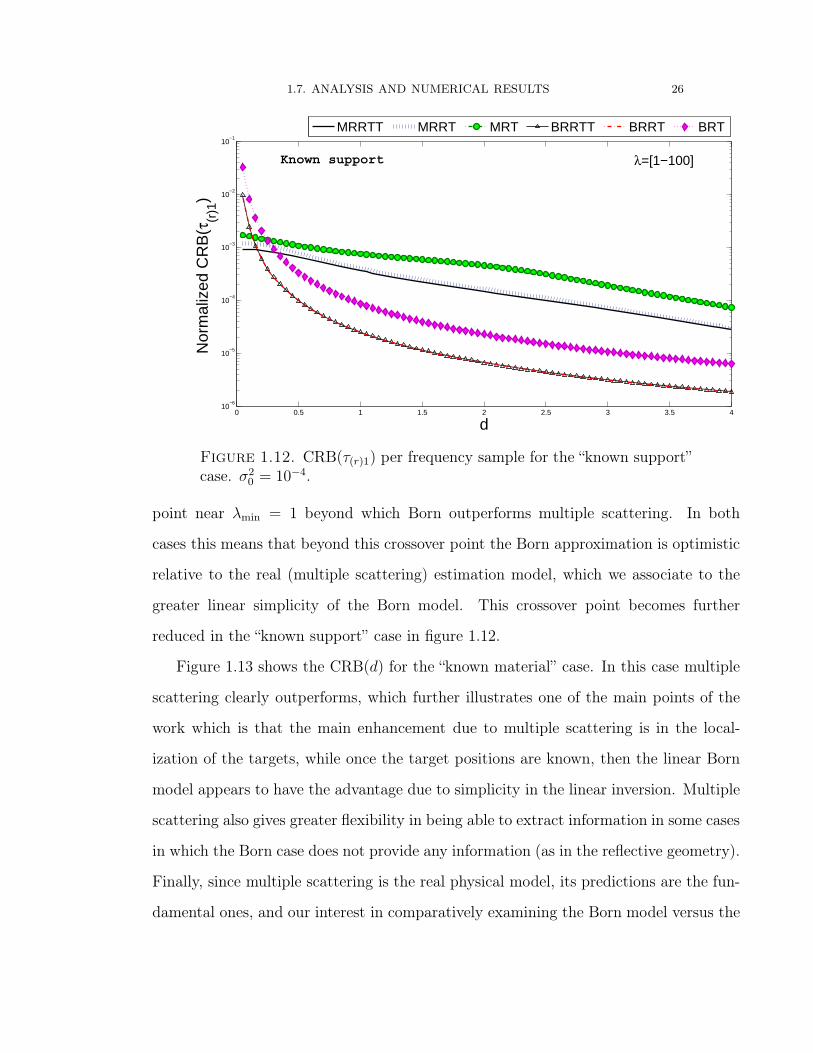
1.7. ANALYSIS AND NUMERICAL RESULTS 26
0 0.5 1 1.5 2 2.5 3 3.5 410
−6
10−5
10−4
10−3
10−2
10−1
d
Nor
mal
ized
CR
B(τ
(r)1
)
MRRTT MRRT MRT BRRTT BRRT BRT
Known support λ=[1−100]
Figure 1.12. CRB(τ(r)1) per frequency sample for the “known support”case. σ2
0 = 10−4.
point near λmin = 1 beyond which Born outperforms multiple scattering. In both
cases this means that beyond this crossover point the Born approximation is optimistic
relative to the real (multiple scattering) estimation model, which we associate to the
greater linear simplicity of the Born model. This crossover point becomes further
reduced in the “known support” case in figure 1.12.
Figure 1.13 shows the CRB(d) for the “known material” case. In this case multiple
scattering clearly outperforms, which further illustrates one of the main points of the
work which is that the main enhancement due to multiple scattering is in the local-
ization of the targets, while once the target positions are known, then the linear Born
model appears to have the advantage due to simplicity in the linear inversion. Multiple
scattering also gives greater flexibility in being able to extract information in some cases
in which the Born case does not provide any information (as in the reflective geometry).
Finally, since multiple scattering is the real physical model, its predictions are the fun-
damental ones, and our interest in comparatively examining the Born model versus the

1.8. CONCLUSIONS 27
0 0.5 1 1.5 2 2.5 3
10−4
10−3
d
Nor
mal
ized
CR
B(d
)
MRRTT MRRT BRRTT BRRT
λ=[1−100]Known material
Figure 1.13. CRB(d) per frequency sample for the “known material”case. σ2
0 = 10−4.
multiple scattering model was motivated mostly to understand situations under which
Born is too pessimistic (due to the possibility of better performance thanks to multiple
scattering) or on the contrary too optimistic (thereby giving false expectation of what
can be achieved, as was the tendency in the known support case studies).
1.8. Conclusions
This chapter investigated scattering systems in 1D space in the framework of the
CRB associated with the problem of estimating scattering parameters from the response
of the system as measured using given excitations (transmit experiments) and given
receivers. We adopted the fundamental CRB measure which is algorithm-independent,
i.e., it is a bound on estimation error for any unbiased estimator applied to the given
data.
The 1D geometry is relevant to certain radar and tomographic experiments for
which we considered the full set of bistatic data: reflective and transmissive exper-

1.8. CONCLUSIONS 28
iments. Among other results, we studied the information content of different data
sets, corresponding to different sensing configurations. The Born model gives only low-
spatial-frequency information in the transmissive geometry. It gives more information
in the reflective geometry. The multiple scattering model tends to be more informative
in general (more parameters or at least the same number as in Born can be estimated).
The two reflective geometries (RR) tend to add important new information relative to
the single R. One of the transmissive experiments (single T) also adds noticeable new
information. However, the transmissive geometry is reciprocal under no noise and the
second T experiment, corresponding to the other direction (TT), usually gives only
marginal new information relative to the first T experiment. It was shown that multi-
ple scattering can either enhance or reduce estimation performance, depending on the
system parameters and the particular data used for estimation.
Since (for fixed scattering system parameters) multiple scattering is the correct
model, this means that performance characterizations based on the Born approximation
can be optimistic or pessimistic. Thus multiple scattering may give enhanced resolution
relative to what one would expect under the Born model, but multiple scattering also
implies a more complex nonlinear signal model which can reduce our ability to estimate
parameters. We have illustrated this behavior for many situations above.
As general rule of thumb, it seems that multiple scattering tends to help in the
localization or support estimation problem, but multiple scattering also tends to be
detrimental in estimation of scattering strength alone for known support. Hints of
these general characteristics appeared in the single-frequency illustrations, and became
more notorious in the multi-frequency examples. One generally measures resolution
in terms of the ability of separately locating two nearby small targets, and in this
particular context it seems that multiple scattering does tend to help.
Clearly the simpler 1D case has provided a new corroboration of known facts in
this area as well as a lot of new intuition into the role of multiple scattering and of

1.8. CONCLUSIONS 29
different configurations in yielding information about scattering systems from their re-
sponse matrix. However it is important to establish how the scattering characteristics
of the system (targets position and strength) interplay to control the estimation capa-
bility under both models. This relationship is examined further, both theoretically and
computationally, in chapter 2.

CHAPTER 2
Cramer-Rao Bound Analysis Under Elastic Scattering
Using the signal model defined in Section 1.1, one collects noisy data which depend
on the remote sensing configuration (R, T, RT, etc.). In Section 1.5 we considered
different vectors ξ corresponding to different combinations of the following parameters:
The position X1 of target 1, the target separation d, the real and imaginary parts τ(r)m
and τ(i)m of target strength τm, m = 1, 2, and the unknown noise variance σ20. This
large parameter space gave complicated expressions that had to be solved numerically,
thereby rendering limited insight into the connection between the estimation perfor-
mance and conditions of our system (parameters and sensing configuration associated
to the scattering matrix K). In the present chapter the focus is the elastic scattering
regime, which reduces the dimensionality of the parameter space. Further reduction of
the parameter space is defined by assuming known noise variance σ20 .
2.1. Elastic Scattering Condition
In 1D space, under energy-conservative, elastic scattering, the scattering strengths
τm obey the condition
(2.28) [Re(τm)]2 + Re(τm) + [Im(τm)]
2 = 0
where Re and Im denote real and imaginary part, respectively. To arrive at this result,
one notes that in the present scalar wave context, the quantity that is analogous to
the Poynting vector for electromagnetic waves is the energy flux vector ( [33], p. 717)
30

2.2. FISHER INFORMATION MATRIX 31
which in our 1D framework can be expressed in terms of the field ψ(x) as
(2.29) F (x) = β Im
{ψ∗(x)
∂
∂xψ(x)
}where β is a positive constant. Consider a point target having strength τ . Let exp(ikx)
be the incident field, so that the field to the left of the target is exp(ikx)+ τ exp(−ikx)while the field to the right of the target is (1 + τ) exp(ikx). Then the energy flux to
the left is F (x < 0) = βk(1 − |τ |2), while the energy flux to the right is F (x > 0) =
βk[1+2Re(τ)+ |τ |2]. In elastic scattering the flux remains continuous at the scattering
interface so that k(1 − |τ |2) = k[1 + 2Re(τ) + |τ |2], which gives (2.28), as desired.
Furthermore, it can be shown that, consequently, the most general scattering strength
τ which gives rise to elastic (non-dissipative) scattering is of the form
(2.30) τ = − cos(θ) exp(iθ)
where θ ∈ [−π/2, π/2].
2.2. Fisher Information Matrix
Using Eq.(2.30), we have τ1 = − cos θ1 exp {iθ1}, τ2 = − cos θ2 exp {iθ2} and σ20 is
known, so that the parameter vector
(2.31) ξ = [x1, d, θ1, θ2]T
The corresponding Fisher information matrix(FIM) I(ξ) and the CRB lower bound
(CRB[ξ(i)]) for the variance var[ξ(i)] of any unbiased estimator for the parameter ξ(i)s
are defined by equation(1.22).
In the following, rather than computing the full FIM above, we focus on the diagonal
elements of that matrix. This defines a conditional FIM for each parameter, and the
associated CRB, under prior knowledge of the other parameters. Furthermore, from the

2.2. FISHER INFORMATION MATRIX 32
properties of the FIM, the resulting diagonal-approximated FIM, and resulting FIM,
also renders an approximation to the CRB resulting from the full FIM (including the
off-diagonal, cross-information terms).
Importantly, due to statistical independence, the FIM of R and/or T data sets, e.g.,
RRT (both reflective experiments, and one transmissive experiment), is given by the
sum of the individual (R,R,T) FIM’s, e.g., IRRT = IR(−,−)+ IR(+,+)
+ IT(+,−). Therefore
our analysis of the single-R and single-T data cases applies to larger sets of R and/or
T data.
The fact of estimate just one parameter at the time reduces the complexity associ-
ated to this problem and provides insight into the relation between targets locations,
reflectivities and frequency. This method represents the exact FIM just for one param-
eter.
Note that the FIM of one parameter quantifies the significance of choosing some
characteristics of the system to enhance the estimation for single or multiple frequency
cases. This special case also allow us to distinguish the conditions under each model
enhances o diminishes the estimation of one parameter. Therefore, the optimal next
experiments are identified.
2.2.1. Diagonal Entry I(ξ)1,1: Estimation of X1. The CRB of the first scat-
terer position X1 goes infinity when the case T is used for the estimation of the position
of the first scatterer because the transmissive experiment has no information about X1.
It will be convenient to gain insight plus facilitate interpretation to introduce qm =
iτm = τm/2k for m = 1, 2, natural parameters that appears repeatedly in the present
CRB analysis of scattering systems.
For the case R under the Born approximation model, the FIM is obtained using the
definition in Eqs.(1.22) and simplifying terms, we get the result:

2.2. FISHER INFORMATION MATRIX 33
(2.32) I (X1)BornR−,− =
2
σ20
{|q1|2 + |q2|2 + 2� [q∗1q2 exp (i2kd)]}= I (X1)
BornR+,+
In the multiple scattering model, one obtains
I (X1)MSR−,− =
2
σ20
{|q1|2 + |q2|2
(1 + 2 [q1] + |q1|2
)21 + 2� [q1q2 exp(i2kd)] + |q1|2 |q2|2
}
+2
σ20
{2�[q∗1q2
exp (i2kd)(1 + 2 [q1] + |q1|2
)(1 + q1q2 exp (i2kd))
]}(2.33)
where ∗ denotes complex conjugation. This result also gives the corresponding result
for the reflective R+,+ case via the substitutions q1 → q2 and q2 → q1.
2.2.2. Diagonal Entry I(ξ)2,2: Estimation of d. In this case of the estimation
of the separation between the two targets “d”, the Born approximation model again
presents same result for the two different sensing points. The FIM under Born for the
reflective case R is defined by:
(2.34) I (d)BornR−,− =
2
σ20
|q2|2 = I (d)BornR+,+
From the Eq.(2.34), it can be seem that the CRB for the scatterers’ separations "d"
under the Born approximation model is linear dependent of the natural parameter q2
and the noise of the system.
For multiple scattering model, the reflective data point R−,−produces the following
FIM:
(2.35) I (d)MSR−,− =
2
σ20
|q2|2{ (
1 + 2 [q1] + |q1|2)2(
1 + 2� [q1q2 exp (i2kd)] + |q1|2 |q2|2)2}

2.2. FISHER INFORMATION MATRIX 34
The FIM for the reflective case R+,+ is defined by:
I (d)MSR+,+
=2
σ20
|q2|2{1 + 2�
[(1− iq2)
2 q21 exp (i4kd)
(1 + q1q2 exp (i2kd))2
]}
+2
σ20
|q2|2{
|q1|4(1 + 2 [q2] + |q2|2
)2[1 + 2� [q1q2 exp (i2kd)] + |q1|2 |q2|2
]2}
(2.36)
For the transmissive case under Born approximation model, the first derivative with
respect to "d " vanish, therefore the FIM for the case T is zero. Contrarily, the multiple
scattering model presents the following FIM:
(2.37)
I (d)MST+,− =
2
σ20
{|q1|2 |q2|2
(1 + 2 [q1] + |q1|2
) (1 + 2 [q2] + |q2|2
)[1 + 2� [q1q2 exp(i2kd)] + |q1|2 |q2|2
]2}
= I (d)MST−,+
where I (d)MST+,− = I (d)MS
T−,+due to non dispersive media property again.
The expressions for X1 and d above are written in function of q1 = τ1/2k and
q2 = τ2/2k. Those expressions also apply to any type scattering not only elastic.
The Born approximation and the multiple scattering models for the reflective cases
have some similar characteristics in each components of the expressions of FIM in
the estimation of scatterers positions (d and X1). In most of the cases, the multiple
scattering model have a multiplicative factor that depends on the natural parameters
q1, q2, and exp(i2kd) which illustrate the difference between them.
In the expressions of the FIM for parameters d and X1 above, the frequency plays
a determinant role being part of the "natural parameters" of the systems. As the fre-
quency increases the FIM become small then the CRB will be larger. Consequently
qm � 1 and both models will have a equivalent result in the estimation of the one
parameter however with large level of errors. This in turn indicates scattering condi-
tions under which the Born-approximation-based estimation performance estimates are

2.2. FISHER INFORMATION MATRIX 35
pessimistic (optimistic). In d estimation, it appears that the scattering strength of the
scatterer that is closer to the receiver has a significant role. In particular, numerical
results based on eqs. (2.32) through (2.37) (results not shown) show that FIM under
multiple scattering tends to increase as the scattering strength of the scatterer that is
closer to the receiver increases.
The transmissive case "T" for the estimation of X1 will not contribute information
for both models. This situation remains for estimation of the scatterers separation d
under the Born approximation model. The transmissive case T for multiple scattering
contributes noticeably in the estimation of d if both natural scatterers reflectivities qm
are quite large.
2.2.3. Diagonal Entries I(ξ)3,3 and I(ξ)4,4: Estimation of θ1 and θ2. In the
estimation of the scatterer’s reflectivity, without loss of generality the variable to esti-
mate will be θn, which immediately can be related with error bounds of the real and
imaginary part of the strength of the target τm for elastic case.
The FIM for case R under the Born approximation model is given by:
(2.38) I (θ1)BornR−,− =
2
σ20
{1
(2k)4
}The equation (2.38) holds for any reflective and transmissive case for the estimation
of strength of the target. This expression also remains in case of estimation of any
scatterer reflectivity under the Born approx. model. Thus I (θ1)BornR = I (θ1)
BornT and
I (θ1)BornR or T = I (θ2)
BornR or T .
The equation (2.38) indicates that under Born approximation model, the error
bounds for the estimation of the scatterer’s reflectivities only depends on the noise
variance and the wavelength instead of the reflectivity and position of the targets.
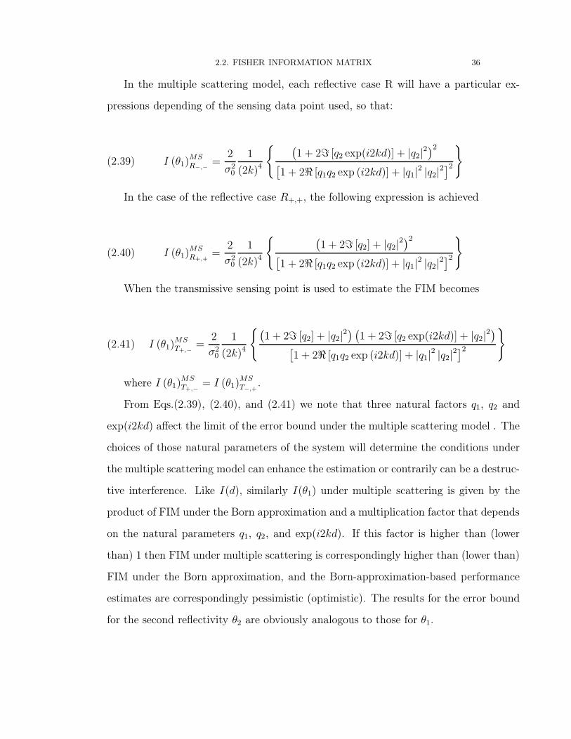
2.2. FISHER INFORMATION MATRIX 36
In the multiple scattering model, each reflective case R will have a particular ex-
pressions depending of the sensing data point used, so that:
(2.39) I (θ1)MSR−,− =
2
σ20
1
(2k)4
{ (1 + 2 [q2 exp(i2kd)] + |q2|2
)2[1 + 2� [q1q2 exp (i2kd)] + |q1|2 |q2|2
]2}
In the case of the reflective case R+,+, the following expression is achieved
(2.40) I (θ1)MSR+,+
=2
σ20
1
(2k)4
{ (1 + 2 [q2] + |q2|2
)2[1 + 2� [q1q2 exp (i2kd)] + |q1|2 |q2|2
]2}
When the transmissive sensing point is used to estimate the FIM becomes
(2.41) I (θ1)MST+,− =
2
σ20
1
(2k)4
{(1 + 2 [q2] + |q2|2
) (1 + 2 [q2 exp(i2kd)] + |q2|2
)[1 + 2� [q1q2 exp (i2kd)] + |q1|2 |q2|2
]2}
where I (θ1)MST+,− = I (θ1)
MST−,+
.
From Eqs.(2.39), (2.40), and (2.41) we note that three natural factors q1, q2 and
exp(i2kd) affect the limit of the error bound under the multiple scattering model . The
choices of those natural parameters of the system will determine the conditions under
the multiple scattering model can enhance the estimation or contrarily can be a destruc-
tive interference. Like I(d), similarly I(θ1) under multiple scattering is given by the
product of FIM under the Born approximation and a multiplication factor that depends
on the natural parameters q1, q2, and exp(i2kd). If this factor is higher than (lower
than) 1 then FIM under multiple scattering is correspondingly higher than (lower than)
FIM under the Born approximation, and the Born-approximation-based performance
estimates are correspondingly pessimistic (optimistic). The results for the error bound
for the second reflectivity θ2 are obviously analogous to those for θ1.

2.2. FISHER INFORMATION MATRIX 37
2.2.4. Simultaneous Estimation of X1 and d. The preceding results for I(X1)
and I(d) can be further generalized by considering the more general FIM submatrix
IX1,d related to unknown X1 and d and known scattering strengths. After some manip-
ulations, one obtains
IX1,d =2
σ20
⎡⎣ IX1 IX1,d
Id,X1 Id
⎤⎦(2.42)
where IX1 and Id are the diagonal entries of the total FIM that were defined in sub-
sections 2.2.1 and 2.2.2. The off-diagonal element Id,X1 = I∗X1,d. For transmissive data,
IX1,d = 0. For reflective data,
(IX1,d)MSR−− =
[|q2|2
(1 + 2q1 + |q1|2
)[1 + q1q2 exp(i2kd)]
[1 + 2�q1q2 exp(i2kd) + |q1|2 |q2|2
]]
+
[q∗1q2 exp(i2kd)
(1− iq1)2
[1 + q1q2 exp(i2kd)]
](2.43)
and
(IX1,d)MSR++
={|q2|2 + q∗1q2(1 + iq∗2) exp(−i2kd) + q21 |q2|2 (1− iq2)
2 exp(i4kd)}
+
{q1q2 |q1|2
(1 + 2q1 + |q1|2
)2exp(i2kd)
[1 + q1q2 exp(i2kd)][1 + 2�q1q2 exp(i2kd) + |q1|2 |q2|2
]}(2.44)
which for |q1| << 1 and |q2| << 1 reduce to the Born approximation results,
(2.45) (IX1,d)BornR−− =
[|q2|2 + q∗1q2 exp(i2kd)]
and
(2.46) (IX1,d)BornR++
=[|q2|2 + q∗1q2 exp(−i2kd)
].
2.2.5. Complete FIM Matrix for Case RRTT under the Born Approx-
imation. Under elastic scattering, the parameter vector (2.31) is reduced. Both the

2.2. FISHER INFORMATION MATRIX 38
Born approximation model and the more general multiple scattering model are consid-
ered. The CRB for the Born approximation model can be given in closed-form after
long manipulations. In contrast, generally the multiple scattering case does not facili-
tate closed-form results. As an illustrative example of the CRB calculations under the
Born model, consider the case of four measurements (RRTT) corresponding to the full
scattering matrix including for the 1D geometry. In this case the FIM is of the form:
IBornRRTT
(ξ) =2
σ20
⎡⎣ IX1,d(ξ) IX1,d,θ1θ2(ξ)
Iθ1,θ2,X1,d(ξ) Iθ1,θ2(ξ)
⎤⎦(2.47)
where the elements in (2.47 ) are submatrices that represent special cases. The diagonal
2 X 2 submatrices IX1,d(ξ) and Iθ1,,θ2(ξ) represent the FIM under the a priori knowledge
of the scatterers’ strength and the scatterers’ position respectively. The off diagonal
submatrices IX1,d,θ1,θ2(ξ) and Iθ1,θ2,X1,d(ξ) are the cross information when there is no a
priori information of the material and the position of the points targets.
From subsection 2.2.4, IX1,d(ξ) =
⎡⎣ JX1 JX1,d
Jd,X1 Jd
⎤⎦, whose components for case
RRTT are defined by:
JX1 =2
(2k)2{|τ1|2 + |τ2|2 + 2 |τ1| |τ2| cos (2kd)�{exp i (θ1 − θ2)}
}
JX1,d = J∗d,X1
=2
(2k)2{|τ2|2 + |τ1| |τ2| cos (2kd) exp i (θ1 − θ2)
}
Jd =2
(2k)2{|τ2|2}
Similarly, Iθ1,θ2 =
⎡⎣ Jθ1 Jθ1,θ2
Jθ2,θ1 Jθ2
⎤⎦, where

2.3. NUMERICAL ILLUSTRATION 39
Jθ1 = Jθ2 =4
(2k)4
Jθ1,θ2 = J∗θ2,θ1 =
4
(2k)4{cos2 (kd) exp i (2θ1 − 2θ2)
}where ∗ denotes the complex conjugate. The “cross-information” matrices IX1,d,θ1,θ2
,and Iθ1,θ2,X1,d are given by
Iθ1,θ2,x1,d =
⎡⎣ −i2(2k)3
{|τ2| sin (2kd) exp i (2θ1 − θ2)} −i2(2k)3
{|τ2| sin (2kd) exp [i (2θ1 − θ2)]}i2
(2k)3
{|τ1|2 sin (2kd) exp− [i (θ1 − 2θ2)]}
0
⎤⎦where Iθ1,θ2,x1,d = IHx1,d,θ1,θ2
, where H indicates the hermitian.
2.3. Numerical Illustration
In the following numerical experiments, we consider the wavenumber k = 2π/λ for
unit-value λ = 1. In presenting the results for different values of θ1 or θ2, in some of
the plots we consider only the interval (0, π/2) because the corresponding results are
symmetrical to those for (−π/2, 0).Figure (2.1) shows plots of CRB(kd) versus scattering separation (kd), all under
the multiple scattering model, for different data. In this example, τ1 = −0.5 + i0.5
and τ2 = −0.9 + i0.3. Clearly the reflective data dictates the estimation limits. The
transmissive data contributes minimally.
The CRB for θ1 is computed from (2.38), (2.39), (2.40), and (2.41). In addition, one
can also obtain from the same results and the method in [34, pp. 229-233] the CRB for
the real and imaginary parts of τ1. Figure (2.2) shows the corresponding CRB(�(τ1)/k))versus kd. As in figure (2.1), τ1 = −0.5 + i0.5 and τ2 = −0.9 + i0.3. A quasi-resonance
appears in the plot of the CRB as a function of kd. We observe that the cases R and T
individually have, in average, the same error bounds as function of the natural scatterer

2.3. NUMERICAL ILLUSTRATION 40
0 0.2 0.4 0.6 0.8 1 1.2 1.4 1.6 1.8 210
−1
100
101
102
kd(π)
CR
B(k
d)
MRMTMRTMTTMRRMRRTMRRTT
Figure 2.1. CRB(kd) including multiple scattering, versus kd, for σ20 =
10−4, for data sets R, T, RR, TT, RT, RRT and RRTT.
separation kd, although the plot reveals that for kdε (.596π − 1.007π) the case R(−,−)
is better. Similar characteristics remains for case R(+,+) not shown. As more sensing
data are added, the error bound for the first scatterer reflectivity decreases. The “next
optimal data” (R or T) to estimate the scatterer reflectivity can be either reflective or
transmissive because the CRB’s with the same number of samples show comparable
results, see, e.g., for example, the cases RR, RT and TT in the figure.
To elucidate the regions in scattering parameter space where multiple scatter-
ing enhances or diminishes the CRB relative to the Born approximation reference
model, we plot in the following the ratio of the Fisher information of the two models,
I(ξ)MS/I(ξ)Born. When this quantity is above 1 the Born approximation estimation
performance estimates are pessimistic, while when it is below 1 the Born approximation
estimates are optimistic. When I(ξ)MS/I(ξ)Born � 1 both models coincide in information-
carrying capacity about ξ.
Figures (2.3) and (2.4) show the ratio I(d)MS/I(d)Born for different reflective data. In
figure (2.3a) the I (d) ratio is shown as a function of the scatterers strength θ1 and θ2,

2.3. NUMERICAL ILLUSTRATION 41
0 0.2 0.4 0.6 0.8 1 1.2 1.4 1.6 1.8 2
10−2
10−1
kd(π)
CR
B(�
(τ1)/
k)
MR MT MRT MTT MRR MRRT MRRTT
Figure 2.2. CRB(�(τ1)/k) including multiple scattering, versus kd, forσ20 = 10−4, for data sets R, T, RR, TT, RT, RRT, and RRTT.
for d = 0.25λ for data set R(−,−). The dark regions in the plot correspond to regions
where both models coincide in estimation capabilities. The other areas illustrate the
enhancement of multiple scattering in the estimation for scatterers separation d. Figure
(2.3b) shows the ratio of the I(d) for reflective data R(+,+) for d = 0.15λ. We can identify
regions with ratio less than one. This means the Born approximation model presents a
smaller error bound than the real multiple scattering model.
Figure (2.4) illustrates the behavior of I(d)MS/I(d)Born versus θ and d, in the case
when both scatterers have the same reflectivity, θ1 = θ = θ2. Each data set shows
a different behavior. For the reflective data set R(−,−), the scatterers reflectivity θ
is dominant in controlling when multiple scattering enhances or diminishes estima-
tion. From figure (2.4a), approximately for θ � 0 multiple scattering enhances infor-
mation about d. In contrast, as seen in figure (2.4b), for the data set R(+,+) both
parameters d and θ play an important role in the estimation. Approximately, for
(−0.2π � θ � 0.2π)⋂
(0.22λ � d � 0.35λ) multiple scattering enhances the estimation.
The behavior of the ratio I (θ1) versus θ2 and d is shown in figure (2.5). The top
2.4. CONCLUSIONS 42
(a), middle (b), and bottom (c) plots forming this figure correspond to cases R(−,−) ,
R(+,+), and T , respectively. Each data set shows a different behavior. The dark region
in (a), (b), and (c) corresponds to diminished estimation due to destructive multiple
scattering. On the other hand, the regions where multiple scattering significantly en-
hances estimation are, approximately: 0.25λ � d � 0.5λ for R(−,−) in part (a), θ2 � 0
for R(+,+) in part (b), and {θ2 � 0}⋂ {0.25λ � d � 0.5λ} for T in part (c).
2.4. Conclusions
This chapter investigated the application of the fundamental estimation-theoretic
Cramer-Rao bound, which gives the lower bound for the error variance of unbiased esti-
mation of scattering parameters from scattering matrix data. Attention was restricted
to scattering systems in 1D space with special interest in describes the connections be-
tween the information capabilities and the scattering parameters of the system for Born
approximation and the most general multiple scattering model. Particular emphasis was
given to systems of small (point-like) elastic scatterers for which the complex-valued
scattering strength is described by a single scattering parameter.
To further maintain the focus, we considered the special case of two scatterers for
which the total number of parameters is four (two positions and two angles describing
the individual scattering strengths) under the elastic conditions. This focus allowed
closed form expressions for special cases. Of much interest are the diagonal elements of
the FIM, for which closed form expressions were derived. Quite often the inverse of the
FIM which defines the CRB is essentially dominated by the diagonal elements of FIM.
This calculation is also relevant in special cases when one has a priori information
in scatterer position and/or scattering strength, and the different diagonal elements
correspond to different physical situations or applications.
It was found that certain natural parameters, in particular, qm = τm/2k, consistently
appear in all the CRB calculations. The information content in reflective (R) data is

2.4. CONCLUSIONS 43
usually better than transmissive (T) data, particularly in position or separation distance
estimations, but that they are comparable in certain cases, particularly in scattering
strength estimation. We developed our results for both signal models, to comparatively
study the role of multiple scattering in either enhancing or diminishing estimation
performance from scattering data. This gives an good indication of the performance
estimates based on the Born approximation model and establishes parametric conditions
under which such estimates are applicable, or in contrary, are either clearly optimistic
or pessimistic. Optimistic and pessimistic regions in parameter space were illustrated.
Thus contrary to the focus in several recent papers [9,14], which emphasize the positive
role of multiple scattering in enhancing imaging, we have provided counterexamples
where multiple scattering is detrimental relative to weak scattering imaging despite the
greater contrast of highly scattering targets.
It is important to point out that the 1D case is also important in its own right, e.g.,
our multiple scattering results (which are algorithm-independent since they are based on
the CRB approach) provide light on the role of multiple scattering among different cross
sections of an object under investigation via tomographic experiments for cross sections
that exhibit slow spatial variation relative to the wavelength (as in x-ray tomography)
but where unlike most (linearizing) models the multiple scattering interactions including
backscattering by different cross section planes are not neglected. Also, even though
we have emphasized for conceptual simplicity the case of point scatterers, in reality a
similar formulation applies to extended objects having uniform constitutive properties
(like a wall) after substitution of our scattering strength coefficients for reflection and
transmission coefficients that depend on the mismatch between the wall and the free
space medium, as is well known (for example, see [30, pp.220-223]).

2.4. CONCLUSIONS 44
Figure 2.3. I(d)MS/I(d)Born for reflective data versus the scatteringstrengths θm for m= 1,2, under scatterer separation d = 0.25λ in (topplot) and d = 0.15λ (bottom plot), with σ2
0 = 10−4. The top plot corre-sponds to R(−,−), while the bottom plot corresponds to R(+,+).

2.4. CONCLUSIONS 45
Figure 2.4. I(d)MS/I(d)Born for reflective data versus θ and d, whenboth scatterers have the same reflectivity. The top and bottom plotscorrespond to the cases R(−,−) and R(+,+), respectively.

2.4. CONCLUSIONS 46
Figure 2.5. I(θ1)MS/I(θ1)Born versus θ2 and d. The top left, top right,and bottom plots correspond to the cases R(−,−), R(+,+) and T , respec-tively

CHAPTER 3
Cramer-Rao Bound Analysis of Scattering Systems in
Three-dimensional Space
This chapter extends some of the CRB results of the previous chapters to the three-
dimensional case. The focus is the case of two point scatterers located along the z axis,
which serves to investigate the role of multiple scattering in resolution and other related
questions.
3.1. The Forward Scattering Mapping
We consider scattering systems in the context of the scalar Helmholtz operator in
three-dimensional space. The incident fields Ψ(i)(r) obey the Helmholtz equation in the
background medium of interest, in particular,
(3.48)(∇2 + k2
)Ψ(i)(r) = 0,
where k = 2π/λ is the wavenumber of the field corresponding to wavelength λ. In the
presence of scatterers or inhomogeneities to the background medium, characterized by
scattering potential V (r), the total field Ψ(r) obeys
(3.49) (∇2 + k2)Ψ(r) = V (r)Ψ(r).
The scattering potential is given by V (r) = k2−κ2(r) where κ(r) denotes the wavenum-
ber of the field in the total medium including the scatterers.
From (3.48, 3.49) the scattered field,
(3.50) Ψ(s)(r) = Ψ(r)−Ψ(i)(r),
47

3.1. THE FORWARD SCATTERING MAPPING 48
obeys
(3.51)(∇2 + k2
)Ψ(s)(r) = V (r)Ψ(r).
The solution of (3.51) obeying outgoing wave boundary conditions for the scattered
field is given by
(3.52) Ψ(s)(r) =
∫d3r′V (r′)Ψ(r′)G (r− r′)
where G (r− r′) is the outgoing Green function of the Helmholtz operator, which is
given by
(3.53) G (r− r′) = − 1
4π
eik|r−r′|
|r− r′| .
In the far field where r � r′, we can approximate |r− r′| � r − s.r′, where r = |r|and s = r/r. Then the far-field approximation for Green’s function is
(3.54) G (r− r′) ∼ − 1
4πreikre−iks.r′
which upon substitution in (3.52) yields the expression for the far scattered field
(3.55) Ψ(s)(r) ∼ − 1
4π
eikr
rf(s; Ψ(i)
)where the quantity f
(s; Ψ(i)
)is the far-field scattering amplitude and is given by
(3.56) f(s; Ψ(i)
)=
∫d3r′V (r′)Ψ(r′)e−iks·r′.
For weak scattering, wherein Ψ(r) � Ψ(i)(r), the result (3.56) reduces to the (first)
Born approximation form
(3.57) f(s; Ψ(i)
)=
∫d3r′V (r′)Ψ(i)(r′)e−iks·r′

3.1. THE FORWARD SCATTERING MAPPING 49
which for the important case of incident plane wave excitation where Ψ(i)(r) = eiksi·r
reduces further to
(3.58) f(s; Ψ(i)
)=
∫d3r′V (r′)e−ik(s−si)·r′.
For point targets we consider the Foldy-Lax multiple scattering model (see, e.g.,
Ysanget al. [35],pp.379) where the scattered field is given by the discrete counterpart
of (3.52),
(3.59) Ψ(s)(r) =M∑
m=1
τmΨ(Rm)G (r−Rm) ,
so that the total field is given by the discrete form of (3.50,3.52),
(3.60) Ψ(r) = Ψ(i)(r) +
M∑m=1
τmΨ(Rm)G(r−Rm),
valid everywhere, except at the target positions where
(3.61) Ψ(Rm) = Ψ(i)(Rm) +∑n �=m
τnΨ(Rn)G(Rm −Rn).
By using (3.54) in the expressions (3.59,3.61) that define the scattered field one arrives at
(3.55) where the corresponding scattering amplitude is given by the discrete counterpart
of (3.56),
(3.62) f(s; Ψ(i)) =M∑
m=1
τmΨ(Rm)e−iks·Rm.
Let us focus on a system of two point scatterers having complex scattering strengths
τ1 and τ2, and positions R1 = (0, 0, d1) and R2 = (0, 0, d2), in the z axis. We assume
d2 > d1. Let the target separation d = d2 − d1 > 0. Consider incident plane waves
eiksi·r with incidence polar angle α (cosα = si · z) and far-zone sensing at scattering
angle β (cos β = s · z).

3.1. THE FORWARD SCATTERING MAPPING 50
For this two-scatterer system, and under plane wave excitation, expression (3.61)
yields the system of equations
Ψ(R1) = eikd1 cosα + τ2Ψ(R2)G0(d)
Ψ(R2) = eikd2 cosα + τ1Ψ(R1)G0(d)(3.63)
where G0(d) =−eikd
4πdand whose solution is given by
Ψ(R1) = F(d, τ1, τ2)[eikd1 cosα(1 + τ2G0(d)e
ikd cosα)]
Ψ(R2) = F(d, τ1, τ2)[eikd1 cosα(τ1G0(d) + eikd cosα)
]where the quantity
(3.64) F(d, τ1, τ2) =
(1
1− τ1τ2G20(d)
)is due to multiple scattering and will play an important role in the Cramer-Rao study
to follow.
The scattering amplitude including multiple scattering takes the form
f(s; Ψ(i)
)=eikd1(cosα−cos β)
1− τ1τ2G20(d)
× [τ1 + τ2eikd(cosα−cos β)
+τ1τ2G0(d)(eikd cosα + e−ikd cos β)](3.65)
For the special case of weak scatterers this takes the Born approximation form
(3.66) f(s; Ψ(i)
)= eikd1(cosα−cos β)
[τ1 + τ2e
ikd(cosα−cos β)]
In these expressions the angles α and β lie in the range [0, π]. This will be used
next to define different cases of interest.

3.2. ELASTIC SCATTERING CONDITION IN 3D SPACE 51
3.2. Elastic Scattering Condition in 3D Space
In the 3D scattering system, the elastic scattering condition is given by
(3.67) k([Re(τm)]
2 + [Im(τm)]2)− Re(τm) = 0
To show this, we consider the energy flux vector [33] which in the 3D case can be
expressed in terms of the field as
(3.68) 〈F(r)〉 = −iβ [Ψ∗(r)∇Ψ(r)−Ψ(r)∇Ψ∗(r)]
where β is a positive constant and Ψ(r) is the total field, hence
(3.69) 〈F(r)〉 = ⟨F(i)(r)⟩+⟨F(s)(r)
⟩+⟨F
′(r)⟩
where⟨F(i)⟩,⟨F(s)⟩, and
⟨F
′⟩ are the average flux energy due to the incident wave,
the scattering field and the iteractions between both waves, respectively. Therefore the
outward flow through a surface of a large sphere Σ of radius R is given by
(3.70) W =
∫Σ
〈F(r).ndΣ〉
where n is the unit outward normal to Σ.
Consider a point target spherically symmetric of scattering strength α. The asso-
ciated scattered field due to an incident field exp(iks0.r) (where s0 is the direction of
incidence) behaves in the far zones (kR → ∞) as
(3.71) Ψ(Rs) ∼ αexp(ikR)
R
where s is the unit vector in the direction of the observation point. The scattering
amplitude α remains the same for all incidence directions (due to spherical symmetry of
the scatterer) and scattering directions (due to the small size of the scatterer which gives

3.3. CRAMER-RAO BOUND ESTIMATION 52
rise to isotropic radiation due to any incident field). Due to law of energy conservation
the net of energy flux through the surface is equal to the absorption. Then the energy
flux W is zero for nonabsorbing medium, so that
(3.72) W = W (i) +W (s) +W′= 0
where W (i), W (s) and W ′ are the outward flow corresponding Eq.(3.69) where W (i) = 0
because the incident field satisfy the Helmholtz equation. By using the Eqs.(3.69,3.71),
we have
(3.73) W = 2βk(4π |α|2)− 8πβα = 0
which satisfy the elastic condition in (3.67). Furthermore, the most general scattering
strength α is of the form
(3.74) α =ei2Φ − 1
i2k
where Φ ∈ [0, 2π].
3.3. Cramer-Rao Bound Estimation
Considering additive complex Gaussian noise, the signal model is
K(ξ) = K (ξ) +W
where K is the noise-free data vector, K is the collected noisy data vector, ξ is the
estimated parameter vector, and W is complex Gaussian noise with variance σ20.
Assuming that the noise variance σ20 is known then in general, we define the param-
eter vector:
(3.75) ξ = [d1, d,�τ1,τ1,�τ2,τ2]T ,

3.3. CRAMER-RAO BOUND ESTIMATION 53
where � and denote the real and imaginary parts, respectively. Under elastic scat-
tering (non-dissipative), the target reflectivity must obey the condition in Eq.(3.74).
Thus, the vector parameter for τ1 = τ2 is given by
(3.76) ξ = [d1, d, φ]T
More specialized cases of analytical and practical interest are the estimation of d1 under
prior knowledge of the other parameters, i.e.,
(3.77) ξ = d1
which simulates a canonical target localization problem including internal multiple scat-
tering at the two-target system, and the estimation of the two-target separation d (the
targets’ resolution) under prior knowledge of the strengths and the reference position
d1, in particular,
(3.78) ξ = d.
Another analytically tractable and practically important case is the estimation of the
target strengths under prior knowledge of the target positions (simulating the practi-
cal inverse scattering problem after the target support has been estimated). Further
reductions of the parameter space apply for special cases such as elastic scatterers, as
we shall consider later in the paper. From (3.65)
(3.79) Ki,j(ξ)=eikd1(cosαi−cos βj)[1− ei2kd
(4πd)2τ1τ2
] [τ1 + τ2eikd(cosαi−cos βj) − τ1τ2
eikd
4πd(eikd cosαi+e−ikd cos βj)]
for i = 1, 2, . . . , Nt incident waves and j = 1, 2, . . . , Nr sensing points. In the following
we consider the vectorized or stacked form of K (ξ), i.e., K (ξ) is the NtNr × 1 vector
formed by the entries Ki,j(ξ), i = 1, 2, · · · , Nt; j = 1, 2, · · · , Nr. Similarly we arrange
the corresponding NtNr data entries Ki,j, i = 1, 2, · · · , Nt; j = 1, 2, · · · , Nr into the

3.3. CRAMER-RAO BOUND ESTIMATION 54
NtNr × 1 data vector K. The respective Born approximation is given from (3.66) by
(3.80) KBorni,j (ξ) = eikd1(cosαi−cos βj)
[τ1+τ2e
ikd(cosαi−cos βj)].
A fundamental measure of the estimability of the parameters of interest, ξ, from
the noisy data is the Cramér-Rao lower bound or CRB. The CRB, CRB(ξi), of the
parameter ξi, constitutes a lower bound, achievable under mild conditions, for the
variance var(ξi) = E[(ξi − ξi)2] (where E denotes the expected value) of any unbiased
estimate ξi of the parameter ξi. It is given by the diagonal elements of the so-called
Fisher information matrix (FIM) [7, eq.3.20]
(3.81) var(ξi) ≥ [I−1(ξ)]i,i = CRB(ξi)
where the FIM I(ξ) is given by [7, eq.15.52]
(3.82) I(ξ)i,j=2�[∂KH(ξ)
∂ξiC−1
˜K(ξ)
∂K(ξ)
∂ξj
]
where H denotes the conjugate transpose, and C˜K is the covariance matrix [7, pp. 501]
which in our case is simply C˜K = σ2
0I. Here I denotes the NtNr×NtNr identity matrix.
Therefore (3.82) reduces to
(3.83) I(ξ)i,j = 2σ−20 �
[∂KH(ξ)
∂ξi(ξ)
∂K(ξ)
∂ξj
]
or equivalently to the sum of the FIM of all the observations, in particular,
(3.84) I(ξ)i,j =
Nt∑m=1
Nr∑n=1
I(m,n)i,j (ξ)

3.3. CRAMER-RAO BOUND ESTIMATION 55
where I(m,n)i,j is the FIM of the (m,n) scattering experiment, for incidence angle αm and
scattering or sensing angle βn, which is given by
I(ξ)m,ni,j = 2σ−2
0 �[∂K∗
m,n(ξ)
∂ξi
∂Km,n(ξ)
∂ξj
]
= 2σ−20
[∂�{Km,n(ξ)}
∂ξi
∂�{Km,n(ξ)}∂ξj
+∂{Km,n(ξ)}
∂ξi
∂{Km,n(ξ)}∂ξj
](3.85)
Also the derivative of the noisy scattering amplitude could be computed as [29]
(3.86)∂K(ξ)
∂ξi=∂∣∣∣K(ξ)
∣∣∣∂ξi
ei∠˜K(ξ) + i
∂∠K(ξ)
∂ξi
∣∣∣K(ξ)∣∣∣ ei∠ ˜K(ξ)
We may further simplify the CRB(ξi) in the form [36],
(3.87) CRB(ξi) =[I(ξ)i,i − ud,ξi−1
I−1(ξ)i−1uHd,ξi−1
]−1
where I(ξ)i,i is the Fisher score function for the parameter ξi, I(ξ)i−1 is the FIM matrix
for the remaining (i− 1) parameters, and ud,ξi−1is the vector 1× (i− 1) with the cross
information terms defined by
ud,ξi−1=
2
σ20
�{∂KH
∂ξi
(∂K
∂ξ1...
∂K
∂ξi−1
)}
In addition, it is not hard to show that
(3.88) CRB(ξ) ≥ [I(ξ)i,i]−1
with equality holding if ξ is a scalar, e.g., if the target strengths and separation are
known but the position d1 is unknown (two-target system localization).
We focus in the following on the diagonal entries of the FIM, to obtain approxi-
mate analytical insight on the information content of scattering data, which applies via
(3.88) as lower bound for the CRB itself, or as the exact CRB when only one scattering

3.3. CRAMER-RAO BOUND ESTIMATION 56
parameter is estimated (scalar ξ). Therefore, rather than consider the full FIM matrix,
which is more difficult to compute analytically, and harder to interpret, we develop
in the following closed form expressions for the diagonal components of the FIM for
canonical situations simulating target localization, the estimation of target separation
(resolution), and inversion of the scattering strengths for known target positions (in-
verse scattering problem). This task is more analytically tractable, and still gives a
lot of insight about the information about scattering parameters in scattering data.
The results of this work generalize to the 3D case the corresponding 1D results of a
recent conference paper [16]. Of particular interest is to gain insight about the impact
that the separation distance between the targets d, the target strengths τ1, τ2, and the
sensing configuration have in the estimation of scattering-based systems, which renders
further understanding about the intrinsic limits of scattering parameter estimability
under the general multiple scattering regime, and also helps to design optimal exper-
iments relevant to radar, sonar, and wireless communications in multiple scattering
environments.
3.3.1. Scatterer Position “d1”: Localization. This calculation characterizes the
information about the scatterer position, for a known scatterer formed by two point
scatterers with given strengths τ1 and τ2 and separation distance (d). From a radar or
sonar point of view, the question is up to what point the localizability of the two-point
scatterer target is affected by the target parameters τ1, τ2, d, and the particular remote
sensing configuration (in the present case, the angles (α, β) for which scattering data
are collected). One may intuitively expect weak scatterers to be harder to locate (due
to lower signal-to-noise ratio (SNR)) than strong scatterers involving (internal) multiple
scattering. However the following results show that multiple scattering can diminish
SNR and thereby also the target localizability in certain regions of scattering parameter
and sensing configuration spaces while it can enhance it in others.

3.3. CRAMER-RAO BOUND ESTIMATION 57
The Fisher information I(d1) is given by Eq.(3.84) where the Fisher information
I(m,n)(d1) of the (m,n) experiment is evaluated by applying Eq.(3.85) to the signal
models in Eqs.(3.79) and (3.80). For the Born approximation model based on (3.80)
one obtains
(3.89) I(m,n)(d1)Born = 2k2g2(αm, βn)SNRBorn(αm, βn)
where
(3.90) g(α, β) = cos(α)− cos(β)
and
(3.91) SNRBorn(α, β) =∣∣τ1 + τ2e
ikdg(α,β)∣∣2 /σ2
0.
For the more general multiple scattering model based on (3.79) one obtains
(3.92) I(m,n)(d1) = 2k2g2(αm, βn)SNR(αm, βn)
where
SNR(α, β) =|F (d, τ1, τ2)|2
σ02
{σ20SNRBorn(α, β) + �
[τ1τ24πd
Q(d, α, β)(τ ∗1 + τ ∗2 e
−ikdg)]
+2 |τ1|2|τ2|2(4πd)2
[1 + cos(kd(cosα + cos β))]
}(3.93)
where
(3.94) |F (d, τ1, τ2)|2 = 1[1− 2�
{τ1τ2
ei2kd
(4πd)2
}+ |τ1|2|τ2|2
(4πd)4
]and
(3.95) Q(d, α, β) = eikd cosα + e−ikd cos β.

3.3. CRAMER-RAO BOUND ESTIMATION 58
The latter result reduces to the Born approximation result (3.91) for small |τmG0(d)| <<1, m = 1, 2, as expected.
In general, in both the exact multiple scattering context and the Born approximation
contexts, the Fisher information I(m,n)(d1) and therefore the associated localizability of
the two-target system is seen to depend on the respective SNR and the difference of
cosine term g(αm, βm) given by (3.90). The latter depends only on the sensing configu-
ration (the incidence and scattering or sensing angles). For the sensing configurations
where g = 0, in particular, the line-of-sight experiments where α = β, it is not possible
to extract information about the two-target system location from the scattering data,
this being the case for both weak and strong scattering systems. However, if one cap-
tures non-line-of-sight data then g �= 0 and one may deduce the sought-after location.
For a given α, the sensing configuration term (g2(α, β)) is maximized if β = π for
α ∈ [0, π/2), if β = 0 for α ∈ (π/2, π], and if β = 0 or π for α = π/2. And with these
values of β, the values of α giving the largest g2 = 4 are α = 0 (with β = π) and α = π
(with β = 0), which correspond to special cases of backscattering-based sensing where
β = π − α as in monostatic radar and sonar systems. On the other hand, the exact
multiple scattering model SNR is seen from the general results Eqs.(3.93,3.94,3.95) to
be proportional to the (d, τ1, τ2)-dependent factor |F (d, τ1, τ2)|2 in (3.94). Hence one
expects that maximization (minimization) of this scattering-parameter-dependent fac-
tor enhances (diminishes) localizability. The Born approximation model result (3.91)
does not have this factor and, in addition, involves only the first of the three terms
in the outer parenthesis of the more general result (3.93). Thus the SNR differs in
the exact versus approximate models. In the exact model it depends through F on
the scattering parameters (d, τ1, τ2) and, in a more complex manner, through the large
multiplicative parenthesis term in (3.93), on both the scattering parameters and the
sensing configuration.
We discuss next some results which illustrate the type of interesting insight about the

3.3. CRAMER-RAO BOUND ESTIMATION 59
information content of scattering data and the combined roles of scattering parameters
and sensing configuration that can be gained from the Fisher information/CRB analysis,
by discussing the issue of blind data spots as applicable to Born approximation and
exact multiple scattering models. First we emphasize that no information about the
location is contained in line-of-sight data, and this holds for both exact and approximate
models. Another situation when the experiment does not render information is when
due to the combined role of scattering parameters and sensing configuration the SNR
happens to vanish. Within the Born approximation model, the zero SNR condition,
SNRBorn(α, β) = 0, is from (3.91)
(3.96) τ1 + τ2eikdg(α,β) = 0.
There are infinite values of the scattering parameters and the sensing angles for which
this condition is obeyed. In particular, the constraint Eq.(3.96) requires |τ1| = |τ2|, and
if this holds the condition becomes
(3.97)
kdg(α, β) = kd(cosα− cos β) = θ1 − θ2 + lπ, l = ±(2n + 1), n = 0, 1, 2, · · · , nmax
where the real-valued θ1, θ2 are the phase angles of τ1, τ2, i.e., τ1 = |τ1|eiθ1, τ2 = |τ2|eiθ2 .Since the maximum value of |g(α, β)| = 2, then the maximum value nmax of integer
index n in (3.97) is constrained by |(θ1 − θ2)/π ± (2n+ 1)| ≤ 4d/λ, i.e.,
(3.98) (2nmax + 1)2 ± (2nmax + 1)(θ1 − θ2)/π + (θ1 − θ2)2/π2 ≤ 16(d/λ)2.
For example, if τ1 = τ2 then from (3.97) if the condition kdg(α, β) = lπ, l = ±(2n +
1), n = 0, 1, 2, · · · , nmax holds, then SNRBorn(α, β) = 0. Given any choice of the
angles α, β, the target separations d = (2n+ 1)λ/[2|g(α, β)|] > 0, n = 0, 1, 2, · · · ren-
der zero SNR, SNRBorn(α, β) = 0. Alternatively, for any separation distance d, then
SNRBorn(α, β) = 0 for the angles α, β such that g = ± (2n+1)λ2d
, n = 0, 1, 2, · · · , nmax,

3.3. CRAMER-RAO BOUND ESTIMATION 60
where nmax is the largest integer such that nmax ≤ 2d/λ− 1/2. Thus clearly under the
Born approximation model there are values of the parameters and the sensing angles
which can be thought of as “blind spots” for target data acquisition, i.e., they correspond
to zero SNR signals and information. Referring to the more general multiple scattering
model result (3.93) we see that the vanishing of the SNR under the Born approximation
does not imply the corresponding vanishing of SNR under the more general multiple
scattering model. In particular, blind spots under the Born approximation model may
not extend to the multiple scattering regime which can, more generally, still carry infor-
mation about the sought-after parameter, in this case the two-target system location.
Examples of this general situation where the Born approximation offers no information
while the more general multiple scattering model does carry target information are
given later in the numerical illustration section of this paper. Here we wish to continue
this line of discussion by addressing the other related question whether analogous blind
spots exist or not under the more general multiple scattering model. The answer is a
categoric yes, as we detail in the following alongside a simple example.
The question is whether the multiple scattering SNR, SNR(α, β), can also vanish
for certain values of the parameters and the sensing angles. To show this is possible,
consider the second term in (3.93). This term vanishes ifQ defined in Eq.(3.95) vanishes,
which in turn happens if
(3.99) kd(cosα + cos β) = lπ, l = ±(2n + 1), n = 0, 1, 2, · · · .
In turn, this condition automatically causes the vanishing of the third term in (3.93).
Thus if conditions (3.96,3.99) are both obeyed under the constraints | cosα| ≤ 1 and
cos β| ≤ 1, then SNR(α, β) = 0. Equivalently, if |τ1| = |τ2| and conditions (3.97,3.99)
are both obeyed under the constraints | cosα| ≤ 1 and | cosβ| ≤ 1, then SNR(α, β) = 0.

3.3. CRAMER-RAO BOUND ESTIMATION 61
The general condition can be stated as
cosα =λ
4d
[l1 + l2 +
(θ2 − θ1)
π
]cos β =
λ
4d
[l2 − l1 − (θ2 − θ1)
π
]l1 = ±(2n1 + 1), n1 = 0, 1, 2, · · ·
l2 = ±(2n2 + 1), n2 = 0, 1, 2, · · ·
| cosα| =∣∣∣∣λd[l1 + l2
4+
(θ2 − θ1)
2π
]∣∣∣∣ ≤ 1
| cos β| =∣∣∣∣λd[l2 − l1
4+
(θ2 − θ1)
2π
]∣∣∣∣ ≤ 1(3.100)
where as before the real-valued θ1, θ2 are the phase angles of τ1, τ2, i.e., τ1 = |τ1|eiθ1 , τ2 =|τ2|eiθ2. An example is the case τ1 = τ2, and l1 = l = l2, which implies β = π/2, which
further implies d = lλ/(2 cosα) > 0, l = ±(2n + 1), n = 0, 1, 2 · · · . These and related
results are examined further later in the numerical illustration section. It is important
to note that blind spots under the exact multiple scattering modeling automatically
imply the same blind spots in the approximate Born model since then the first term
in (3.93) which is proportional to SNRBorn must also vanish. Then blind spots under
multiple scattering imply the same blind spots under the Born approximation. However,
the converse is not true as we have outlined earlier and as we outline further next for
another sensing scenario.
Finally, another important issue is the implications of these results for the case of
monostatic radar or sonar observations where for a given incidence angle α one captures
data for the backscattering direction associated to β = π − α. In this special case,
condition (3.99) cannot be obeyed, therefore the second and third terms in (3.93) do
not generally vanish. On the other hand, the first term in (3.93) vanishes if condition
(3.97) holds, where in this case cos β = − cosα, and this can in fact happen as we
illustrate in the numerical illustration section. For example, if τ1 = τ2, and d = λ/4,

3.3. CRAMER-RAO BOUND ESTIMATION 62
then for α = 0 (or for α = π) the backscattering SNRBorn(α = 0, π − α = π) = 0
(or SNRBorn(α = π, π − α = 0) = 0). In this case, however, the exact SNR(α =
0, π − α) �= 0 due to the nonvanishing of the second and third terms in (3.93) as we
discuss in the numerical illustration section. Thus while the Born approximation model
may falsely reveal blind spots for backscattering sensing, more generally such blind spots
do not arise in the multiple scattering model. Thus only if the Born approximation
holds, i.e., |τmG0(d)| << 1, m = 1, 2, do the respective backscattering blind spots
approximately apply. This is an example of a situation where multiple scattering can
enhance the sensing capabilities, in this case, the localizability, relative to what one
would have expected from the Born approximation-based model. More implications of
the Fisher information and associated CRB analysis above are discussed alongside plots
in the numerical illustration section. The numerical results include calculations for the
MIMO scenario, where multiple angles are used for both incidence and scattering or
sensing. For this more general situation we employ the result Eq.(3.84) where the Fisher
information I(m,n)(d1) is defined by the expressions given in this section.
3.3.2. Scatterers Separation Distance “d”: Resolution. This part describes
the statistical information that is contained in scattering data about the separation
distance d between two known point scatterers. In imaging systems, the ability to
estimate the separation distance d of two point targets is usually regarded as a metric
for the resolution or ability to resolve target details of the imaging system. The smaller
the separation distance d of two point targets that can be properly estimated, the better
the resolution. The question is how the resolution is affected by the target parameters
τ1, τ2, d, and the remote sensing configuration, particularly in the case when multiple
scattering is significant. In the following we study this question in the exact multiple
scattering framework, and provide conditions under which multiple scattering can be
beneficial or detrimental to resolution, relative to the Born approximation model limits.

3.3. CRAMER-RAO BOUND ESTIMATION 63
In the Born approximation model, the Fisher information I(m,n)(d) is found to be
given by
(3.101) I(m,n)(d)Born = 2σ−20 k2|τ2|2g2(α, β).
On the other hand, in the exact multiple scattering model
(3.102) I(m,n)(d) = 2σ−20 |τ2|2|F |2|A+BF |2
where
A= ikg(α, β)eikdg(α,β) − τ1eikd(1+cosα)
4πd
[ik(1+cosα)− 1
d
](3.103)
−τ1eikd(1−cos β)
4πd
[ik(1−cos β)− 1
d
]B=
τ1ei2kd
(4πd)2
(i2k− 2
d
)[τ1+τ2e
ikdg(α,β)− τ1τ2eikd
4πdQ(d,α,β)
](3.104)
As in the localization problem, in the Born approximation model the Fisher infor-
mation is proportional to g(α, β), which implies that under the condition g = 0 the
target separation d cannot be estimated at all. However, this is not the case under the
multiple scattering model, where according to (3.103,3.104) in general I(m,n)(d) does
not necessarily vanish if g = 0.
Alternatively we may consider another scenario, where the center of the two targets,
dc = (d1 + d2)/2, is known. Physically and informationally, this is a different situation
than the one of the preceding results, and therefore it gives different Fisher information
and CRB results. In particular, in this case we rewrite the signal models Eqs.(3.65)

3.3. CRAMER-RAO BOUND ESTIMATION 64
and (3.66) as
f(α;β) = F (d, τ1, τ2)eikdcg(α,β) ×
[τ1e−ikdg(α,β)/2+τ2e
ikdg(α,β)/2+τ1τ2e−ikdg(α,β)/2G0(d)Q(d,α,β)].
= F (d, τ1, τ2)eikdcg(α,β)[τ1e
−ikdg(α,β)/2+τ2eikdg(α,β)/2+2τ1τ2G0cos(kdg
′/2)].(3.105)
where
(3.106) g′ = cosα + cos β
and
(3.107) f(α; β) � fBorn (α; β) = eikdcg(α,β)[τ1e
−ikdg(α,β)/2 + τ2eikdg(α,β)/2
].
The respective Fisher informations I(m,n)(d) and I(m,n)B (d) can be computed readily.
Computationally they can be shown to exhibit similar behavior to that of the other
approach given earlier.
3.3.3. Scatterers Strength “τ”: Inverse Scattering. We develop further the
statistical information regarding to the scatterers strength for the case of previously
knowledge of the scatterers positions. This problem is well known as an inverse scatter-
ing. Another important question is how the accuracy of the inverse scattering problem
is affected by specific sensing configurations and/or the scattering parameters of the
system when multiple scattering is significant. Due to the difficulty associated to this
problem, we can expect higher error levels in comparisons with the estimation of the
targets position. We simplify the problem by using similar elastic strengths, although
we will explain the connections of our results to complex target strength.
In the case of the estimation of the complex scatterers strength τ , we consider
a complex estimator τ = ˆτ(r) + i ˆτ(i) where [τ(r), τ(i)]T are two real parameter of ξ in

3.3. CRAMER-RAO BOUND ESTIMATION 65
Eq.(3.75). When both estimators ˆτ(r) and ˆτ(i) achieve the minimum variance, τ reaches
the Cramer-Rao lower bound (minimum variance) [37], [7, pp. 527-528]. However this
approach represents that one parameter will be a nuisance parameter of the other,
therefore the error ellipse of ξ increases [34, pp. 231-233]. Consequently, to proceed
with the statistical bound of the scatterers strengths, we find convenient to work with
Φ in the vector parameter in Eq.(3.76) for elastic scattering instead of use the subset
of parameters in Eq.(3.75).
Consider next τ = τ1 = τ2, with scatterer strength τ = (ei2Φ − 1)/i2k Eq.(3.74).
The Fisher information of the scatterers’ reflectivity according to (3.76) is given by:
(3.108) I(Φ)Born =2
k2σ20
(2 + 2 cos [kdg(α,β)]) .
I(Φ)MS =2 |F|4k2σ2
0
(2+2 cos [kdg(α,β)])
[1+2�
{τ 2
ei2kd
(4πd)2
}+
|τ |4(4πd)4
](3.109)
+8 |τ |2 |F|4k2σ2
0(4πd)2(2+2 cos [kd(cosα+ cos β)])
− 8 |F|4k2σ2
04πd
[1+
|τ |2(4πd)2
]�{τQ(d,α,β)[1+e−ikdg(α,β)
]}.
Before proceeding further, we first establish the connection between the CRB of the
elastic parameter Φ with τ(r) and τ(r). We may invoke the chain rules for differentiation
of composite functions τ = (τ(r) + iτ(i)) [29], we get
∂K
∂τ(i)= i
∂K
∂τ(r).
In the case of elastic scattering, when the targets strength obeys Eq.(3.74), we have
(3.110)∂K
∂Φ=∂K
∂τ
∂τ
∂Φ=ei2Φ
k
∂K
∂τ.

3.3. CRAMER-RAO BOUND ESTIMATION 66
According to Eq.(3.110) and the definition in Eq.(3.85), we may write [7],
(3.111) I(τ(r)) = I(τ(i)) = k2I(Φ).
On the basis of Eq.(3.111), we can associate our results to the real and imaginary part
of the elastic strength for a fixed wavenumber k.
Another case of interest is τ = τ(r), we obtain in this case:
(3.112) I(τ(r))Born =
2
σ20
(2 + 2 cos [kdg(α,β)]) .
I(τ(r))MS=
2 |F|4σ20
(2+2 cos [kdg(α,β)])
[1+2�
{τ 2
ei2kd
(4πd)2
}+
|τ |4(4πd)4
](3.113)
+8 |τ |2 |F|4σ20(4πd)
2(2+2 cos [kd(cosα+ cos β)])
−8 |F|4σ204πd
[1+
|τ |2(4πd)2
]�{τQ(d,α,β)[1+e−ikdg(α,β)
]}.
These results agree with the definitions in Eq.(3.111). We can use same approach to
computer the Fisher score for the imaginary part of the targets’ strength.
One notes from Eqs.(3.108),(3.109), (3.112), and (3.113) that our ability to solve
the inverse scattering problem under Born approximation model is affected principally
by the configuration g(α, β) and the separation distance d. Contrarily the multiple
scattering model depends on those parameters as well as how strong are the targets in
a complex non linear way.
3.3.4. Simultaneous Estimation of d1 and d. The preceding results for I(d1)
and I(d) can be further generalized by considering the more general FIM submatrix Id1,d
related to unknown d1 and d and known scattering strengths. After some manipulations,

3.3. CRAMER-RAO BOUND ESTIMATION 67
one obtains
Id1,d =2
σ20
⎡⎣ Id1 Id,d1
Id1,d Id
⎤⎦(3.114)
where Id1 and Id are the diagonal entries of the total FIM that were defined in Eqs.(3.89-
3.102). The off-diagonal element Id1,d = I∗d,d1 , so that
IMSd1,d
=2k2g2(α, β) |F|2
σ20
�{τ2A
(τ1 + τ2e
ikdg(α,β) − τ1τ2eikd
4πdQ(α, β)
)}(3.115)
2kg(α, β) |F|2σ20
�{iτ2BF
(τ1 + τ2e
ikdg(α,β) − τ1τ2eikd
4πdQ(α, β)
)}with F, A and B defined in Eqs.(3.64),(3.103), and (3.104) respectively. For |τ1| << 1
and |τ2| << 1 the previous expression reduces to the Born approximation result,
(3.116) IBornd1,d
=2k2g2(α, β)
σ20
[|τ2|2 + �{τ ∗1 τ2eikdg(α,β)}]When τ1 = τ2 = τ , we apply Eqs.(3.89), (3.101) and (3.116) into Eq.(3.81). After
mathematical manipulation, we get the following result for a single sensing pair (α, β)
(3.117) CRB(d)Born =
[2k2g2(α, β)
σ20
|τ |2 (2 + 2 cos [kdg(α, β)])
]−1
.
For the multiple scattering case, we can use the same procedure. However, it requires
the manipulation of complex mathematical expressions.
3.3.5. Born versus Multiple Scattering Analysis. The essential variation in
information between the Born approximation and multiple scattering model may be
stated as follows: a) the dependence of the characteristics of system (d, τ1, and τ2)
and b) how the position of the transmitter and receiver (α, β) affects the accuracy in
the estimation process. In the first case, the Born approximation model shows small
dependence of d in the estimation of the scatterers strength and only relies on τ2 in the

3.3. CRAMER-RAO BOUND ESTIMATION 68
estimation of the scatterers separation d. Contrarily, multiple scattering shows complex
dependency of all the characteristics of the system.
Like is was mention before the configuration with the line of sight between trans-
mitter and receiver point is critical for the localization of the targets under both models
and the resolution under the Born approximation model in cases of single data experi-
ments or limited scattering data. This special case g(α, β) = 0 belongs to what we call
an ambiguity region conformed |α| = |β| for (α, β ∈ [0, π]). The effect of the sensing
configuration is represented by the cosine of the incident and receiving angles α, β. Of
special importance is the difference of cosine g(α, β) which impacts directly the estima-
tion of the targets positions (d, d1). In particular, the case when g(α, β) = 0 eliminates
the capacity to estimate the position of the first scatterer d1 under both models and
the separation distance d for the Born approximation which occurs when there is line of
sight between transmitter and receiver point. It is important to emphasize that when
the transmissive and observation points are in line of sight, the CRB(d1) will become
infinite. Similar characteristics were described with the transmissive experiment in 1D,
however the 3D case demonstrates that this fact is independent of the targets plane.
The special case g(α, β) = 0 belongs to what we call an ambiguity region conformed
|α| = |β| for (α, β ∈ [0, π]). Under this ambiguity region multiple scattering is still able
to estimate the separation distance d and according to the scattering characteristics of
the system, the estimation error will be low or high. One common way to mitigate this
problem of ambiguity is avoiding the line of sight between the receiver and the trans-
mitter for each pair of probing signal and observation point and using an incoherent
system.
One notes that for targets with equal strength, the error performance in the esti-
mated parameter d1 is worst as d is close to (2n+1)λ2|g(α,β)| for n = 0, 1, . . . where g ∈ [−2, 2]
under the Born approximation model. This result holds for single data experiments.
The effect of this critical distance is diminished as the number of observations increases
3.4. NUMERICAL EXPERIMENTS 69
with different g(α, β), especially as the signal is collected avoiding the line of sight.
On the opposite, the best performance under the Born approximation is found for
d = mλ|g(α,β)| for m = 1, 2, . . . for a single observation. Those critical distances for the
best and worst scenarios under the Born approximation model hold for the estimated
scatterers’ strength (τ or Φ) under similar conditions. However for multiple scatter-
ing the best/worst error performance associated to estimated scatterers’ strength and
position "relies" on the targets strength and their separation jointly with the sens-
ing configuration. Such interpretation for those critical separation d cannot be easily
described for multiple scattering due to its highly non-linear condition. However one
clearly notes that the performance of multiple scattering associated to the statistical
information of d1, d, and τ is highly impacted by the magnitude of F, (Eq. 3.64). The
best error performance of multiple scattering is found for
maxd,τ1,τ2
|F(d, τ1, τ2)|2
which means d, τ1, τ2 values that ensure the maximum signal to noise ratio under multi-
ple scattering and the highest gradient. This not always can be achieved due to physical
limitations of available materials.
3.4. Numerical Experiments
In this section several CRB results are presented and discussed that are pertinent
for the more general multiple scattering signal model. We consider the wavenumber
k = 2π/λ for unit-value λ = 1, and noise variance σ20 = 10−3. We present experimental
results paying attention to CRB dependence on scatterer strength τ and on scatterer
separation d. When the targets strengths obey the elastic scattering condition, τ =
(ei2Φ − 1)/i2k, we focus on presenting the results for different values of Φ, considering
only the interval (0, π) because the corresponding results are symmetrical to those for

3.4. NUMERICAL EXPERIMENTS 70
Figure 3.1. Illustration of a scattering experiment to interrogate twopoint targets.
Figure 3.2. Real and imaginary parts of the target strength under theelastic condition.

3.4. NUMERICAL EXPERIMENTS 71
0 0.1 0.2 0.3 0.4 0.5 0.6 0.7 0.8 0.9 110
−10
10−5
100
105
1010
β(π)
CR
B(d
1)
MS,d=λ/4MS,d=λ/2
Figure 3.3. CRB(d1) as the observation angle β varies with incidentfield at α = 0 for the scatterers’ separation d = λ/4 and d = λ/2.
(−π, 0). Figure 3.2 provides a plot of the real and imaginary part of elastic strength as
Φ varies.
In our results we will present the Born approximation model as a benchmark how-
ever, it is not the principal goal of this work to make a comparative analysis between
both models. We will focus in the real physical multiple scattering model and his effect
in the localization, resolution and inverse scattering problems. Although in case of crit-
ical situations in which there exits marked differences, we will provide some comments.
3.4.1. Estimation of the First Scatterer Position d1: Localization. We ex-
amine first the effect on localization information, as described by CRB(d1), of the
direction of the receiver, β1 = β, for a single-input single-output (SISO) experiment
corresponding to α1 = α = 0. Figure 3.3 shows two plots of CRB(d1) versus β for
α = 0 and τ1 = 1 = τ2. The two plots shown correspond to d = λ/4 and d = λ/2,
respectively. The general tendency is for CRB(d1) to be larger for the small angles β
near zero, and to be smaller for the large angles β near π. Thus it seems that as a rule

3.4. NUMERICAL EXPERIMENTS 72
of thumb one should expect to extract more location information from backscattering
and near-backscattering data, than from forward scattering and near-forward scattering
experiments. However, we also expect from (3.100) that CRB(d1) = ∞ for β = π/2,
and this is in fact the behavior shown in the figure. Thus for d = λ/2, CRB(d1) decays
with β except in the approximate interval (π/3, π/2) where it grows as it reaches a peak
at β = π/2, and then decays steadily beyond π/2 up to π. In contrast, for d = λ/4,
CRB(d1) decays with β in the approximate interval (0, 0.6π) and remains almost con-
stant for β > 0.6π up to π. It is important to note that, as explained in the paragraph
following the discussion of (3.100), under the Born approximation the location infor-
mation vanishes completely for d = λ/4 if β = π. In contrast, as shown in the plot
(which corresponds to the multiple scattering model), for these values (d = λ/4, β = π)
in general the Fisher information does not vanish (and the respective CRB is not in-
finity) under the multiple scattering model. This illustrates an scenario where multiple
scattering enables information that is not present in the Born approximation model.
Figure 3.4 shows plots of CRB(d1) versus α, for SISO experiments giving backscat-
tering data (corresponding to monostatic radar or sonar) where β = π − α. In the
calculations τ1 = 1 = τ2. Plots for both the exact and Born approximation models are
shown, which correspond to the scatterers’ separations d = λ/4 and d = λ/2. The Born
approximation model requires in view of (3.97,3.98) that CRB(d1) = ∞ for α = 0, π
for d = λ/4, and this is the behavior shown in the respective plot (figure 3.4(b)). This
example was discussed in the theoretical section. In addition, the Born approxima-
tion model requires in view of (3.97,3.98) that CRB(d1) = ∞ for α = π/3, 2π/3 for
d = λ/2, and as expected this is the behavior illustrated in the respective plot (figure
3.4(d)). In contrast, the exact model results in figures 3.4(a) and 3.4(c) do not show
these peaks in CRB or blind spots for the extraction of localization information. These
results illustrate concrete situations elaborated in the theoretical discussion where mul-
tiple scattering is necessarily beneficial. In particular, as explained in the discussion

3.4. NUMERICAL EXPERIMENTS 73
0 0.1 0.2 0.3 0.4 0.5 0.6 0.7 0.8 0.9 110
−10
10−5
100
105
1010
α(π)
CR
B(d
1)
MS,d=λ/4
(a)
0 0.1 0.2 0.3 0.4 0.5 0.6 0.7 0.8 0.9 110
−10
10−5
100
105
1010
α(π)
CR
B(d
1)
Born,d=λ/4
(b)
0 0.1 0.2 0.3 0.4 0.5 0.6 0.7 0.8 0.9 110
−10
10−5
100
105
1010
α(π)
CR
B(d
1)
MS,d=λ/2
(c)
0 0.1 0.2 0.3 0.4 0.5 0.6 0.7 0.8 0.9 110
−10
10−5
100
105
1010
α(π)C
RB
(d1)
Born,d=λ/2
(d)
Figure 3.4. CRB(d1) as the incident angle α varies with observationangle at β = π − α for the scatterers’ separation d = λ/4 and d = λ/2.Subfigures (a) and (c) correspond to the real multiple scattering modelwhile subfigures (b) and (d) to the Born approximation model.
following (3.100), under backscattering, if SNRBorn(α, π − α) = 0 (CRB(d1) = ∞)
then necessarily the exact SNR(α, π − α) �= 0 (finite CRB(d1)). By comparing figure
3.4(a) with figure 3.4(b) we notice that CRB(d1) under the exact model is consistently
smaller than that for the Born approximation, the difference being more drastic near
the axis (angles close to α = 0, π) where the aforementioned infinity of CRB(d1) under
the Born approximation occurs. On the other hand, by comparing figure 3.4(c) with
figure 3.4(d) we notice that the values of CRB for the two models are comparable for a
broad range of angles, with the most marked differences (where the exact model is much
better) occurring near the angles α = π/3, 2π/3 where the CRB becomes infinite under
the Born approximation. However, these plots also show that there are sensing angles
for which the Born approximation prediction is better, which corresponds of course to

3.4. NUMERICAL EXPERIMENTS 74
0 0.1 0.2 0.3 0.4 0.5 0.6 0.7 0.8 0.9 110
−8
10−7
10−6
10−5
10−4
10−3
d(λ)
CR
B(d
1)
#10 #20
Figure 3.5. CRB(d1) as scatterers’ separation d varies. Plots are gen-erated using Nr = Nt where α, β ∈ (0, π).
0 0.05 0.1 0.15 0.2 0.25 0.3 0.35 0.4 0.45 0.510
−2
100
102
104
106
108
d(λ)
1/|F
|2
CRB(d1)MS ∝ 1/|F |2
Figure 3.6. Plot of 1/|F|2 with τ1 = τ2 = 1.
an optimistic expectation since the exact multiple scattering model is the real physical
one.
The results discussed so far apply to SISO sensing scenarios. We consider next

3.4. NUMERICAL EXPERIMENTS 75
multiple-input multiple-output (MIMO) sensing scenarios, corresponding to discrete
sets of incidence and scattering angles. Figure 3.5 shows plots of CRB(d1) versus d
(in λ) for scattering data corresponding to MIMO experiments using Nt = 10 and 20
incidence angles αm, m = 1, 2, · · · , Nt that are evenly spaced in the interval [0, π], and
Nr = 10 and 20 scattering angles βn, n = 1, 2, · · · , Nr that are evenly spaced in the
same interval. The line-of-sight experiments (α = β) do not contribute localization
information and are not included. As expected, as more data are gathered, the Fisher
information becomes larger and the corresponding CRB decreases. Despite showing
different fluctuations, the plots for the different numbers of samples show the same
general behavior where the CRB is large for small targets’ separation d, and fluctuates
much more slowly for d in the broad range from λ/10 to λ. Figure 3.6 shows the behav-
ior of the term 1/|F (d, τ1, τ2)|2 which, according to Eqs.(3.92,3.93), is proportional to
CRB(d1). Clearly the general behavior of this term coincides with that of CRB(d1) for
the cases considered, which suggests that this term is quite dominant in controlling the
Fisher information and CRB for the MIMO sensing with the full angular range [0, π]
for both incidence and scattering directions. We consider in the following other exper-
iments where the angular ranges are narrower, being of particular interest situations
corresponding to near-forward scattering in the endfire direction or array axis (small
incidence and scattering angles), to near-backscattering in the endfire direction (small
incidence angles and large scattering angles), to forward or backward scattering near
the broadside angle (angles near π/2), as well as to probing in either near endfire or
near broadside directions followed by sensing in the other (near broadside or endfire)
directions.
Figure 3.7 shows the results of MIMO experiments in the near-forward scatter-
ing directions, near the endfire or array axis. The figure shows the dependence of
CRB(d1) versus d for MIMO experiments corresponding to Nt = 20 incidence angles
αm, m = 1, 2, · · · , Nt, and Nr = 20 scattering angles βn, n = 1, 2, · · · , Nr, where the

3.4. NUMERICAL EXPERIMENTS 76
0 0.1 0.2 0.3 0.4 0.5 0.6 0.7 0.8 0.9 110
−8
10−6
10−4
10−2
100
d(λ)
CR
B(d
1)
θe=π/16 θ
e=π/8 θ
e=π/4 θ
e=π/2 Born θ
e=π/2
Figure 3.7. CRB(d1) as scatterers’ separation d varies. Plots are gen-erated using Nr = Nt = 20 evenly spaced in the angular region α, β ∈(0, θe).
angles are uniformly spaced in the angular region [0, θe], where θe takes the values
θe = π/16, π/8, π/4, π/2. For reference, also shown in the figure is the corresponding
curve for the Born approximation model for θe = π/2. Clearly as the angular range
increases the CRB decreases. In addition, the CRB for the Born approximation model
approximates very well the true CRB for d larger than approximately λ/4. Below that
point, the multiple scattering and Born approximation plots diverge with the multiple
scattering CRB increasing rapidly as d becomes smaller.
Figure 3.8 corresponds to MIMO experiments in the near-backward scattering di-
rections, near the endfire or array axis. In this case the CRB levels are much lower
than those for the near-forward scattering data in figure 5. Unlike the results in figure
3.7, in this case larger angular region does not imply lower CRB. Thus it seems the
experiments closer to the strict backscattering direction have more information density.
For example, for approximately d ≤ 0.65λ, the smaller the angular range the smaller
the CRB. The Born approximation results for θe = π/2 are very similar to the exact
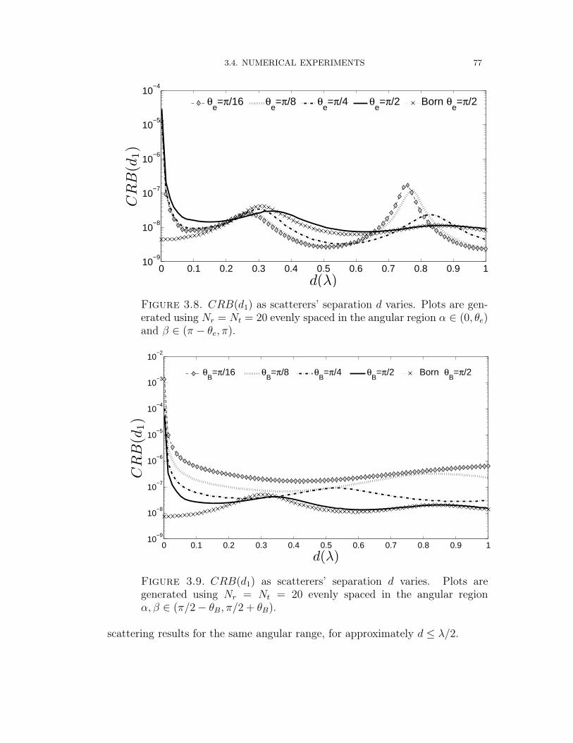
3.4. NUMERICAL EXPERIMENTS 77
0 0.1 0.2 0.3 0.4 0.5 0.6 0.7 0.8 0.9 110
−9
10−8
10−7
10−6
10−5
10−4
d(λ)
CR
B(d
1)
θe=π/16 θ
e=π/8 θ
e=π/4 θ
e=π/2 Born θ
e=π/2
Figure 3.8. CRB(d1) as scatterers’ separation d varies. Plots are gen-erated using Nr = Nt = 20 evenly spaced in the angular region α ∈ (0, θe)and β ∈ (π − θe, π).
0 0.1 0.2 0.3 0.4 0.5 0.6 0.7 0.8 0.9 110
−9
10−8
10−7
10−6
10−5
10−4
10−3
10−2
d(λ)
CR
B(d
1)
θB=π/16 θ
B=π/8 θ
B=π/4 θ
B=π/2 Born θ
B=π/2
Figure 3.9. CRB(d1) as scatterers’ separation d varies. Plots aregenerated using Nr = Nt = 20 evenly spaced in the angular regionα, β ∈ (π/2− θB, π/2 + θB).
scattering results for the same angular range, for approximately d ≤ λ/2.

3.4. NUMERICAL EXPERIMENTS 78
10−3
10−2
10−1
100
101
10−10
10−9
10−8
10−7
10−6
10−5
10−4
10−3
τ2
CR
B(d
1)
d=0.01λd=0.02λd=0.1λd=0.5λ
Figure 3.10. CRB(d1) as the scatterer strength τ2 increases under theBorn approximation and the multiple scattering model for different tar-gets’ separation d. Plots are generated using a sensing configuration with10 probing fields and 10 receivers point (α, β ∈ (0, π)) with τ1 = 1.
Figure 3.9 corresponds to MIMO experiments in the near-broadside directions. The
figure shows the dependence of CRB(d1) versus d for MIMO experiments corresponding
to Nt = 20 incidence angles αm, m = 1, 2, · · · , Nt, and Nr = 20 scattering angles
βn, n = 1, 2, · · · , Nr, where the angles are uniformly spaced in the angular region [π/2−θB, π/2 + θB], where θB takes the values θB = π/16, π/8, π/4, π/2. For reference, also
shown in the figure is the corresponding curve for the Born approximation model for
θB = π/2. In this case the CRB levels consistently decrease as the angular region
becomes larger. As in the previous MIMO examples, the Born approximation results
are similar to the exact scattering model results for θB = π/2, except for small d below
λ/4.
Figure 3.10 illustrates the dependence of CRB(d1) on target strength τ2, for fixed
τ1 = 1. The plot corresponds to the MIMO sensing scenario involving Nt = 20 uni-
formly sampled incidence angles αm, m = 1, 2, · · · , Nt in the interval [0, π] and Nr = 20

3.4. NUMERICAL EXPERIMENTS 79
uniformly sampled scattering angles βn, n = 1, 2, · · · , Nr in the interval [0, π]. The line-
of-sight experiments (α = β) are included. For very small d the dependence of CRB(d1)
on τ2 is quite marked for small values of τ2, revealing sharp local maximum and mini-
mum peaks. As d becomes moderately large (d ≥ 0.1λ) the CRB varies little with τ2
approximately below 0.5, and decays steadily beyond that point. Thus for moderate
values of d the effect of adding the scatterer seems to be positive (towards reducing
the CRB) particularly for large τ2. For very small d the dependence is more complex,
exhibiting noticeable local maximum and minimum peaks for τ2 approximately below
0.5.
In summary, these numerical results show that under broad angle MIMO data, in
which the effect of the particular sensing configuration is somehow averaged, the Born
approximation model seems to approximate well the exact multiple scattering results
for values of d ≥ λ/4, but that for d < λ/4 the difference between the two is very
marked. For d < λ/4 the exact model predicts that the CRB steadily increases as d
decreases, while under the Born approximation the CRB varies little for d ∈ (0, λ/4].
Thus it seems the difference between the Born approximation and exact scattering
models becomes more visible for specific SISO configurations where the role of the
configuration can be decisively in favor (as enhancer of the CRB) of one or the other
model. In the theoretical discussion and the above SISO results we provided explicit
examples of cases where the multiple scattering model yields lower CRB. However, the
plots also show that in certain configurations it is the Born approximation model which
renders lower CRB. However, even in those cases, the multiple scattering result is not
that far from the respective Born approximation result. Thus it seems that overall
multiple scattering enhances localizability under certain SISO conditions, in particular,
due to its immunity to Born approximation blind spots. On the other hand, the MIMO
results show that for small d the effect of multiple scattering is consistently detrimental
to localizability, thus for large scattering data sets and small separations d the effect of

3.4. NUMERICAL EXPERIMENTS 80
0 0.05 0.1 0.15 0.2 0.25 0.3 0.35 0.4 0.45 0.510
−3
10−2
10−1
d(λ)
√ CR
B(d
)/d2
α=0,β=0
α=π/2,β=π/2
Figure 3.11. Resolution√CRB(d)/d2 as d increases with τ1 = τ2 = 1
under the multiple scattering model.
multiple scattering appears to be destructive relative to the Born approximation whose
associated predictions are therefore optimistic.
3.4.2. Estimation of the Scatterers’ Separation d: Resolution. When we
estimate the scatterers’ separation d, we present our results in terms of the relative
resolution [2],
γd =
√CRB(d)
d2.
We start with the study of a single incident single output experiment with the
objective to clarify how the targets plane could affect the resolution under the real
multiple scattering model. Figure 3.11 shows γd as a function of d with τ1 = τ2 = 1.
The scattering data are collected using a single incident direction and observation for the
particular case when the incident and receiving point are in line of sight. In general it
look like the resolution is deteriorated as d increases. Note also that the performance is
better when the targets plane is transversal (α = β = π/2) to the sensing configuration

3.4. NUMERICAL EXPERIMENTS 81
0 0.05 0.1 0.15 0.2 0.25 0.3 0.35 0.4 0.45 0.510
−3
10−2
10−1
100
101
102
d(λ)
√ CR
B(d
)/d2
1 2 5 10 50 100 1000
Figure 3.12. Resolution√CRB(d)/d2 versus d as the number of ob-
servations increases with τ1 = τ2 = 1. The observations are collected inthe interval of scattering directions β ∈ [0 − π/4] with α = 0 under theBorn approximation model.
compared with the longitudinal case (α = β = 0) with the exemption of the interval
0.06λ � d � 0.14λ.
One wonder how will be affected the resolution as the number of scattering data
increases. For this case we will use a single incident field and increment the receiving
points under a specific interval of reception under same conditions. Figure 3.13 shows
γd as a function of d for different number of observations for τ1 = τ2 = 1 when the
data are collected in the scattering directions interval β ∈ [0, π/4]. The data points
are uniformly spaced (equally spaced samples in the interval of interest). As expected,
we note lower CRB as more samples are collected. We note that CRB(d) decreases
around 0.5, 1, and 1.5 dB when the scattering data corresponds 10, 100, and 1000
angular observations respectively. In general we observe the trajectories will be similar
with better performance as the amount of data increase independently of the non linear
complex relation between the parameter and the information associated to its.

3.4. NUMERICAL EXPERIMENTS 82
0 0.05 0.1 0.15 0.2 0.25 0.3 0.35 0.4 0.45 0.5
10−3
10−2
10−1
100
d(λ)
√ CR
B(d
)/d2
1 2 5 10 50 100 1000
Figure 3.13. Resolution√CRB(d)/d2 versus d as the number of ob-
servations increases with τ1 = τ2 = 1. The observations are collected inthe interval of scattering directions β ∈ [0 − π/4] with α = 0 under themultiple scattering model.
Next a comparison of the resolution γd for different sensing intervals is illustrated in
figure 3.14 as the targets’ separation d increases. The goal is illustrated how the sens-
ing configuration impact the resolution and the difference in only using forward and
back scattering data. Hence we study the lower error bound of the targets’ separation
distance CRB(d) (γd) versus d considering four intervals of observation, β ∈ (0, π/4),
β ∈ (π/4, π/2), β ∈ (π/2, 3π/4), β ∈ (3π/4, π), corresponding to a “single-transmit
multiple receive” or “single-input multiple-output” (SIMO) experiment. It is worth not-
ing that as the angular difference between receivers and transmitter angles increases
the resolution increases (CRB(d) decreases). This means that, generally, the larger
the available backscattering data the better the achievable resolution (for example
.16λ � d � 0.5λ). However as the scatterers get closer the resolution could become
necessarily worse or better. Physical intuition about this result is given by the Born
approximation model, wherein the backscattered data corresponds to high frequency

3.4. NUMERICAL EXPERIMENTS 83
0 0.05 0.1 0.15 0.2 0.25 0.3 0.35 0.4 0.45 0.5
10−3
10−2
10−1
100
d(λ)
√ CR
B(d
)/d2
MS,β(0−π/4)MS,β(π/4−π/2)MS,β(π/2−3π/4)MS,β(3π/4−π)
B,β(0−π/4)B,β(π/4−π/2)B,β(π/2−3π/4)B,β(3π/4−π)
Figure 3.14. Resolution√CRB(d)/d2 versus d with τ1 = τ2 = 1 for
different observation intervals. The plots are generated using 100 obser-vations collected using a single incident field (α = 0) under both the Bornapproximation and the multiple scattering model.
Fourier components of the object in the extended Ewald sphere while the forward scat-
tering data are related to the low frequency components.
Under Born approximation the resolution decays monotonically with d. Also, it
becomes more difficult to estimate their separation or distinguish them in small sub-
wavelength separation distances when backscattering data is used. In contrast, in the
multiple scattering case we notice regions of subwavelength separation wherein estima-
tion error for d is comparable to or lower than that of the half-wavelength separation.
This means that at least under certain conditions, the estimation of subwavelength sep-
aration is comparable to that of the half-wavelength case which is used as a reference for
super-resolution studies. Also the contrary case it is exposed that multiple scattering
could deteriorate the resolution and be much worse than the half wavelength distances.
In particular, figures 3.13 and 3.14 illustrate the most favorable targets separation
interval under multiple scattering where the optimum subwavelength resolution region

3.4. NUMERICAL EXPERIMENTS 84
0 0.05 0.1 0.15 0.2 0.25 0.3 0.35 0.4 0.45 0.510
−4
10−3
10−2
10−1
100
d(λ)
√ CR
B(d
)/d2
B,τ1=τ
2=0.25
MS,τ1=τ
2=0.25
B,τ1=τ
2=1
MS,τ1=τ
2=1
B,τ1=τ
2=1.5
MS,τ1=τ
2=1.5
Figure 3.15. Resolution√CRB(d)/d2 versus d. Plots are generated
using 100 observations collected using different sensing configurations of10 probing field and 10 observations points with α ∈ [0 − π/4], β ∈[3π/4, π].
(lower estimate errors) are exhibited for 0.05λ � d � 0.15λ when using forward scatter-
ing data. However, figure 3.14 also shows in the same region that multiple scattering
deteriorates the resolution when back scattering data is collected (in comparison with
the Born approximation model).
Figure 3.15 illustrates an example for a sensing configuration with 10 probing fields
and 10 receivers points (α ∈ (0, π/4), β ∈ (3π/4, π]) with the same systems characteris-
tic in figure 3.14 where multiple scattering shows a similar performance. Similar to 3.14,
multiple scattering diminishes the resolution when targets are strongest (τ1 = τ2 = 1.5).
Similar characteristic are founded for elastic strength like it is illustrated in figure
3.16 with τ1 = τ2 = 0.0689+0.1194i. However the error performance for elastic scatter-
ers is higher and multiple scattering becomes more similar to the Born approximation
model as d increases.
In order to illustrate the usefulness of using a helper scatter in the resolution, we

3.4. NUMERICAL EXPERIMENTS 85
0 0.05 0.1 0.15 0.2 0.25 0.3 0.35 0.4 0.45 0.510
−3
10−2
10−1
100
101
d(λ)
√ CR
B(d
)/d2
MS,β(0−π/4)MS,β(π/4−π/2)MS,β(π/2−3π/4)MS,β(3π/4−π)B,β(0−π/4)B,β(π/4−π/2)B,β(π/2−3π/4)B,β(3π/4−π)
Figure 3.16. Resolution√CRB(d)/d2 versus d with τ1 = τ2 = 0.0689+
0.1194i for different observation intervals. The plots are generated using100 observations collected using a single incident field (α = 0) under boththe Born approximation and the multiple scattering model.
next examine γd when the second scatterer can be controlled with the idea of enhanc-
ing estimation of d. Therefore we study the resolution γd as the helper strength τ2
increases. After several experiments, it seems than multiple scattering enhances the
resolution when both targets get closer with γ(d) comparable or lower than the half
wavelength separation. However in these same targets’ separation when τ2 � τ1 mul-
tiple scattering deteriorates the resolution. This performs of multiple scattering offers
a range of the magnitude of targets strength (this is limited by physical conditions of
available materials) that could be selected for a helper scatterer (τ2) to ensure a high
resolution when it is placed close to other targets. However, we should consider the ef-
fect of the sensing configuration, especially when the intervals of testing and observation
are limited.
As an example in figure 3.17 shows γd versus τ2 using a sensing configuration with 10
probing fields and 10 observation points. Comparison of the Born approximation and

3.4. NUMERICAL EXPERIMENTS 86
10−3
10−2
10−1
100
101
10−4
10−3
10−2
10−1
100
101
102
τ2
√ CR
B(d
)/d2
B,d=0.01λMS,d=0.01λB,d=0.02λMS,d=0.02λ
B,d=0.1λMS,d=0.1λB,d=0.5λMS, d=0.5λ
Figure 3.17. Resolution√CRB(d)/d2 as τ2 increases with τ1 = 1 for
different scatterers’ separation d. Plots are generated using 100 obser-vations collected using a 10 probing fields and 10 observation points(α, β ∈ [0, π]) under the Born approximation and the multiple scatteringmodel.
the multiple scattering model is provided under different scatterers’ separation d with
τ1 = 1. In the meanwhile multiple scattering outperform Born most of time for d � 0.1λ
showing an optimum resolution around τ2 ≈ 0.016 and τ2 ≈ 0.06 for d = 0.01λ and
d = 0.02λ respectively. When τ1 = 0.1 we found the optimum resolution in τ2 ≈ 0.17
and τ2 ≈ 0.67 for d = 0.01λ and d = 0.02λ respectively (results not shown).
3.4.3. Estimation of the Scatterers’ Strength τ : Inverse Scattering. In
this set of experiments we study the CRB(Φ) for the case of elastic scatterers as the
their separation d increases, assuming previously knowledge of the scatterers’ position
(d1,d). Figure 3.18 (a) illustrates the CRB(Φ) with τ = τ1 = τ2 = 0.0689 + 0.1194i
using 10 receivers points and 10 probing fields for α, β ∈ (0, π). This case represent
when the sensing configuration is not a constraint. The targets’ separation d shows a
minimal effect in the outcome bounds with the exception when the targets get closer

3.4. NUMERICAL EXPERIMENTS 87
with high levels of errors. Figure 3.18 (b) illustrates the CRB(Φ) for the same scatterers’
strengths using 10 receivers points and 10 probing fields for α ∈ (0, π/4), β ∈ (5π/6, π).
Here the sensing configuration have limited testing and observation angles. Contrarily
to the subfigure 3.18 (a), the outcome is highly impacted by d, with high error level
similar when the targets get closer. In general we note small differences for the Born
approximation model and the real physical multiple scattering with the exception of
smallest d. Also high error bounds are observed for both models in comparison with
the estimated for d and d1 under same conditions.
Take into consideration that elastic targets have relative small magnitude,we con-
sider necessary to illustrate the effect with strongest scatterers. To carry out this com-
putation, we assume real scatterers’ reflectivity with τ = τ1 = τ2. This fact simplifies
and allows us illustrate the effect of the separation distance d for dissipative scatterers.
Our result can be extended to a complex strength using the definition addressed in Sub-
section 3.3.3. Contrarily to the elastic case, it exhibits lower bound levels. Similarly,
the multiple scattering seems to reduce or eliminate our estimation capability for close
targets. Figure 3.19 shows the CRB(τ) using 10 receivers points and 10 probing fields
with α ∈ (0, π/4), β ∈ (5π/6, π) for different τ . For this particular example, multiple
scattering enhances the estimation as the scatterers’ strength τ increases. Additionally,
the destructive effect of this particular sensing configurations found in 3.18(b) is exhib-
ited for τ = 0.25 in figure 3.19. However one notes that this effect is minimized as the
strength of the targets increases. The Born approximation keeps his similar response
with respect to d (as illustrated in figure 3.18(b)) and it is not affected by the increment
of the scatterers strength τ .
3.4.4. Comparison of the Statistical Information. In order to illustrate how
the multiple scattering model differs from the Born approximation in terms of the
statistical information associated to the scattering parameter ξ, we evaluate the ratio
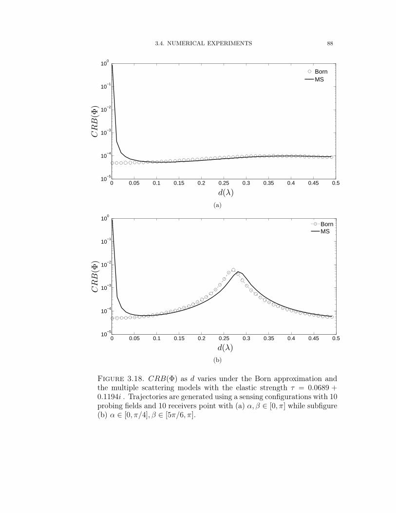
3.4. NUMERICAL EXPERIMENTS 88
0 0.05 0.1 0.15 0.2 0.25 0.3 0.35 0.4 0.45 0.510
−5
10−4
10−3
10−2
10−1
100
d(λ)
CR
B(Φ
)
BornMS
(a)
0 0.05 0.1 0.15 0.2 0.25 0.3 0.35 0.4 0.45 0.510
−5
10−4
10−3
10−2
10−1
100
d(λ)
CR
B(Φ
)
BornMS
(b)
Figure 3.18. CRB(Φ) as d varies under the Born approximation andthe multiple scattering models with the elastic strength τ = 0.0689 +0.1194i . Trajectories are generated using a sensing configurations with 10probing fields and 10 receivers point with (a) α, β ∈ [0, π] while subfigure(b) α ∈ [0, π/4], β ∈ [5π/6, π].
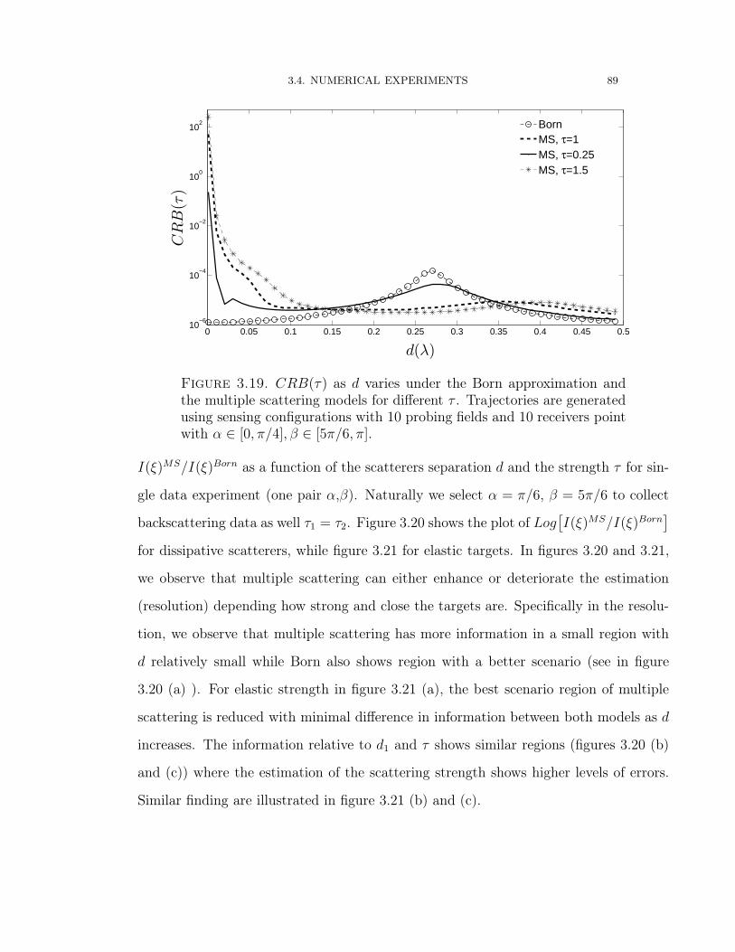
3.4. NUMERICAL EXPERIMENTS 89
0 0.05 0.1 0.15 0.2 0.25 0.3 0.35 0.4 0.45 0.510
−6
10−4
10−2
100
102
d(λ)
CR
B(τ
)
BornMS, τ=1MS, τ=0.25MS, τ=1.5
Figure 3.19. CRB(τ) as d varies under the Born approximation andthe multiple scattering models for different τ . Trajectories are generatedusing sensing configurations with 10 probing fields and 10 receivers pointwith α ∈ [0, π/4], β ∈ [5π/6, π].
I(ξ)MS/I(ξ)Born as a function of the scatterers separation d and the strength τ for sin-
gle data experiment (one pair α,β). Naturally we select α = π/6, β = 5π/6 to collect
backscattering data as well τ1 = τ2. Figure 3.20 shows the plot of Log[I(ξ)MS/I(ξ)Born
]for dissipative scatterers, while figure 3.21 for elastic targets. In figures 3.20 and 3.21,
we observe that multiple scattering can either enhance or deteriorate the estimation
(resolution) depending how strong and close the targets are. Specifically in the resolu-
tion, we observe that multiple scattering has more information in a small region with
d relatively small while Born also shows region with a better scenario (see in figure
3.20 (a) ). For elastic strength in figure 3.21 (a), the best scenario region of multiple
scattering is reduced with minimal difference in information between both models as d
increases. The information relative to d1 and τ shows similar regions (figures 3.20 (b)
and (c)) where the estimation of the scattering strength shows higher levels of errors.
Similar finding are illustrated in figure 3.21 (b) and (c).

3.4. NUMERICAL EXPERIMENTS 90
(a)
(b)
(c)
Figure 3.20. Log[IMS(ξ)/IB(ξ)] as d and τ increase with real targetsstrength τ1 = τ2 = τ . Subfigures (a), (b), and (c) correspond to ξ equalto d, d1, and τ respectively.
3.4.5. Discussion and Further Interpretation. In view of the previous results
in localization, imaging resolution and inverse scattering one naturally wonders: How
different are the scattering waves of both models to lead us to a better or worse outcome?
For this we study the punctual scattering data first (signal as the observation point

3.4. NUMERICAL EXPERIMENTS 91
(a)
(b)
(c)
Figure 3.21. Log[IMS(ξ)/IB(ξ)] as d and Φ increase with elastic targetsstrength τ1 = τ2 = τ = (ei2Φ − 1)/i2k. Subfigures (a), (b), and (c)correspond to ξ equal to d, d1, and τ respectively.
changes) and second scattering data as a function of the targets separation d. For the
first point, we plot the magnitude and phase of the scattering amplitude, as the angle of
observation β varies in figure 3.22, for the particular values of the scattering strengths
τ = 1 for d = 0.08λ and d = 0.5λ under both models (under such conditions d =
0.08λ shows resolution similar to the half-wavelength separation distance or contrarily it

3.4. NUMERICAL EXPERIMENTS 92
0 0.2 0.4 0.6 0.8 10
0.5
1
1.5
2
2.5
β(π)
|K|
MS Born
(a)
0 0.2 0.4 0.6 0.8 1−1
−0.5
0
0.5
1
β(π)
�(K
)
MS Born
(b)
0 0.2 0.4 0.6 0.8 10
0.5
1
1.5
2
2.5
β(π)
|K|
MS Born
(c)
0 0.2 0.4 0.6 0.8 1−1
−0.5
0
0.5
1
β(π)�(K
)
MS Born
(d)
Figure 3.22. Plot of the magnitude and phase of the scattering ampli-tude K versus the angle of reception β with τ1 = τ2 = 1 and α = 0 underthe Born approximation and the multiple scattering model. Subfigures(a) and (b) correspond to the scatterers’ separation d = 0.08λ while (c)and (d) to d = 0.5λ.
represents the worst case). For d = 0.08λ, in figure 3.22(a), we note that the amplitude
of K for Born approximation varies slowly while for multiple scattering is constant.
Contrarily, the corresponding phase plot (figure 3.22(b)) shows large changes with some
differences between both models as the β increases. Subfigures 3.22(c) and (d) show
that both models agree in phase and have small difference between them in amplitude,
so their error bounds have small difference for d = 0.5λ. Those results are based in
punctual plots of the scattering data K for a single probing field at α = 0 which suggest
the phase of the signal plays an important role in the estimation at subwavelength
separations (Eqs. (3.85) and (3.86)).
In the second point, the signal is study as the scatterers’ separation d increases with
a fixed sensing configuration. Figure 3.23 shows the plots of the magnitude and phase

3.4. NUMERICAL EXPERIMENTS 93
of K and the factor F (refer to Eq.(3.64)) which appears in multiple scattering model.
Subfigures 3.23(a) and (b) correspond to α = π/6, β = 5π/6 (back scattering data
collected longitudinal to the targets plane) while 3.23 (c) and (d) to α = π/4, β = π/3
(forward scattering data collected transversal to the targets plane). In the case of
backscattering data (Subfigures 3.23(a) and (b)) we observe marked differences between
both models in amplitude and phase while the forward scattering case shows differences
in amplitude for d � 0.3λ and both model have similar phase. Subfigures 3.23(a) and
(c) shows that multiple scattering have smallest signal when the targets get closer.
This fact is directly traduced in a higher error in localization(it is associated to SNR)
at those smallest d. In the case of the imaging resolution, we can clearly see that it will
affected by both derivatives of the magnitude and phase. In general it important to
observe also that under this experiment with τ1, τ2 = 1, the factor F does not maximize
the magnitude of the signal.
Another interesting study of the signal will be when a helper scatterer (τ2) is in play
to evaluate the connections with the results in figures 3.17 and 3.10 for the resolution
and localization problem respectively. Those results show that multiple scattering could
have much lower error that the half-wavelength separations.
Figure 3.24 illustrates the magnitude and phase of K and F. Subfigures 3.24(a)
and (b) correspond to d = 0.01λ while 3.24(c) and (d) to d = 0.02λ. Subfigures
3.24(a) and 3.24 (c) show the plots of the magnitude of the signal |K| (related to
SNR) is maximum for the same value of τ2 where the factor F(refer to Eq.3.64) have
his maximum amplitude. Those maximum values coincide with the values of τ2 for
the best scenario in the localization problem in figure 3.10. Also we observe as the
magnitude of the signal decreases the localization is limited.
In the case of the resolution, we observe that the derivative of magnitude and phase
are maximum and positive for the same value of τ2 where the best scenario is observed
in figure 3.17. The worst scenario also depends of both derivatives and it is easy to

3.4. NUMERICAL EXPERIMENTS 94
0 0.1 0.2 0.3 0.4 0.50
0.5
1
1.5
2
2.5
d(λ)
|K|
MS Born |F|
(a)
0 0.1 0.2 0.3 0.4 0.5−1
−0.5
0
0.5
1
d(λ)
�K
(π)
MS Born |F|
(b)
0 0.1 0.2 0.3 0.4 0.50
0.5
1
1.5
2
2.5
d(λ)
|K|
MS Born |F|
(c)
0 0.1 0.2 0.3 0.4 0.5−1
−0.5
0
0.5
1
d(λ)�K
(π)
MS Born |F|
(d)
Figure 3.23. Plot of the magnitude and phase of the scattering ampli-tude K as d varies with τ1 = τ2 = 1 under the Born approximation andthe multiple scattering model. Subfigures (a) and (b) correspond to theα = π/6, β = 5π/6 while (c) and (d) to α = π/4, β = π/3.
check these with the help of the definition in Eq.(3.86). We note that the maximum
magnitude of K under multiple scattering occurs at the same maximum amplitude of
F. In the case of the phase, the change in the phase of F coincides with the first large
change in derivative of the phase of K. Definitely in figures 3.17 and 3.10 the best
scenario is directly related with the factor F.
Of great relevance also is the study of the singular value decomposition (SVD)
of the signal using 10 probing fields and 10 observations point spatially distributed
between [0, π] avoiding line of sight . Trajectories are generated as a function of d
under elastic and inelastic conditions. Both systems show an equal number of degrees
of freedom of 2 ( [38]), however we observe variations in the largest singular value σ1
like it is illustrated in figure 3.25. Subfigures (a), (b) correspond to inelastic scatterers

3.4. NUMERICAL EXPERIMENTS 95
10−3
10−2
10−1
100
1010
2
4
6
8
10
τ2
|K|
MS Born |F|
(a)
10−3
10−2
10−1
100
101−1
−0.5
0
0.5
1
τ2
�K
(π)
MS Born |F|
(b)
10−3
10−2
10−1
100
1010
2
4
6
8
10
τ2
|K|
MS Born |F|
(c)
10−3
10−2
10−1
100
101−1
−0.5
0
0.5
1
τ2�K
(π)
MS Born |F|
(d)
Figure 3.24. Plot of the magnitude and phase of the scattering ampli-tude K as τ2 varies with τ1 = 1 under the Born approximation and themultiple scattering model. Subfigures (a) and (b) correspond to d = 0.01λwhile (c) and (d) to d = 0.02λ.
while subfigures (c), (d) to elastic scattering with targets strength τ1 = τ2 = 1 and
τ1 = τ2 = 0.0689 + j0.1194 respectively. For this particular example, we observe under
multiple scattering that σ1 increases for d � 0.25λ until it reaches a value which it is
similar to the Born approximation model for dissipative scatterers. This variation is
less noticeable when the targets strength obeys the elastic condition (figure 3.25(c))
due to the low scattering reflectivity in those cases. The Born approximation model
start with a high singular value for small separation distances and then it decrease as d
increases. It seems that the derivative of the largest singular value of K characterizes
the difference in the information content between both models.

3.5. CONCLUSIONS 96
0 0.1 0.2 0.3 0.4 0.50
5
10
15
20
25
d(λ)
σ1
MS
(a)
0 0.1 0.2 0.3 0.4 0.50
5
10
15
20
25
d(λ)
σ1
Born
(b)
0 0.1 0.2 0.3 0.4 0.50
0.5
1
1.5
2
2.5
3
d(λ)
σ1
MS
(c)
0 0.1 0.2 0.3 0.4 0.50
0.5
1
1.5
2
2.5
3
d(λ)σ
1
Born
(d)
Figure 3.25. Plot of the largest singular value σ1 of K as the scatterers’separation d increases for a sensing configuration of 10 probing fields and10 observation points (α, β ∈ [0, π]). Subfigures (a) and (b) correspondto targets strength τ1 = τ2 = 1, while subfigures (c) and (d) to elasticscatters τ1 = τ2 = 0.0689 + j0.1194.
3.5. Conclusions
This chapter fully investigated the information content associated to an inverse
scattering system in 3D space. The study is carried out in the framework of the CRB
from the given scattering data matrix. Excitation(s) in different directions (probing
fields) interact with the scatterers and the response is measured at different observation
points (receiver points). Particularly, this work shows analytically and numerically
the connections between the errors bound outcomes and scattering parameters of the
system under the most general multiple scattering and the Born approximation. Of
great relevance in our work is the study of the impact that the scattering parameters
and the sensing configuration have in the localization of the targets, imaging resolution

3.5. CONCLUSIONS 97
and solution of the inverse scattering problem.
In general multiple scattering improves the estimation as more backscattering data
is collected when the targets are no really close to each other. Our results also show
that if the scatterers are equal and really close it could deteriorate the error perfor-
mance in sub wavelength distances for all cases (localization of targets, resolution and
inverse scattering) independently of the sensing configuration used. However for dif-
ferent target there are specific sub wavelength separations that could be selected to
find better and worse scenario under multiple scattering. This statement we found is
closely related with the factor F which represents the multiple interactions between
both targets at a specific separation distance when multiple scattering is present. In
general the maximization of F coincides with the best resolution and best scenario in
the localization of the target like our results shown.
Especially important in our work is the study of the impact that the scattering
parameters and the sensing configuration have in the resolution using a definition of
the relative resolution in terms of the information capabilities (CRB) involving two
scatterers [2]. Our work demonstrates how the derivative of the signal of scattering
data plays a key role in the outcome in the resolution under the most general multiple
scattering model. Additional, it is shown that the best resolution that can be obtained
under the Born approximation model occurs at half-wavelength separation distance, in-
dependent of the scattering parameters and the sensing configuration used. Contrarily
multiple scattering achieves similar or even better results when the scattering parame-
ters maximize the signal to noise ratio (F). Another interesting result is how the signal
to noise ratio play a key role in the localization of the targets. However in the inverse
scattering problem, how strong are the targets are a key factor in multiple scattering be
enhancing or diminishing the estimation of the targets strength. Particularly for same
material targets, critical targets separation distances were found for both models where
the estimation is deteriorated in experiments with limited data.

3.5. CONCLUSIONS 98
Among other results, it is demonstrated the key role that play the sensing configu-
ration in the estimation performance particularly under the Born approximation model
where the line of sight between the probing field and the observation point eliminates
his possibility of estimation any position. On the contrary, we are still able to estimate
the targets’ separation under multiple scattering. This result agrees with our work in
1-D space in [16, 18, 19]. However the 3D case shows that such phenomenon is in-
dependent of the targets plane. For large amount of data, the sensing configuration
in the outcome related to multiple scattering could deteriorate the outcome with high
error performances similar when the targets are really close. This occurs when limited
intervals of transmission and reception angles are used to collect the data. This effect
is reduced as more data is selected but more important it can be neglected when we
measure the entire space (α, β ∈ [0, π]).
In general, when a helper or artificial scatterer is used to improve or enhance our es-
timation/imaging capability, our study shows that multiple scattering model not always
appears as constructive information. Contrarily, it could be a destructive interference
depending of the scattering parameters as our numerical experiments exhibit. The 3D
case is important because shows how multiple scattering is a natural encoding mech-
anism that can enable the extraction of high frequency (or high resolution) near field
encoded information about an object or scatterer into the scatterer data. The same in-
formation cannot be recovered from far field measurement if scattering does not include
multiple scattering (without the factor F). Specifically our study shows the necessary
conditions in terms of scattering parameters and the sensing configuration to enable a
low or high estimation error under multiple scattering. Additionally, this special case
of two scatterers is relevant because it allows us to establish the connections between
resolution and the physical characteristics of a system (scattering parameters and sens-
ing configuration) which in the conventional diffraction limit is only associated to the
separation d = λ/2.

3.5. CONCLUSIONS 99
To finalize, this work shows in 3D dimension space that multiple scattering can
be used to design the best optimal experiment especially in application with minimal
resources like in geophysical testing, chemical engineering, biomedical imaging, radar, or
in any kind of non destructive/invasive experiments where the number of observations
is limited. Analytically is demonstrated that multiple scattering is able to resolve two
targets in situations where the sensing configuration is a constraint (ambiguity regions).
Contrarily it can be used as tool in radar to limit or do not allow the localization of
our targets. Specifically multiple scattering can be applied to improve the imaging
resolution for coherent transmissive experiments. All these applications require a detail
design because multiple scattering also could diminish the resolution for small distances.

CHAPTER 4
Compressive Coherent Optical Imaging
4.1. Generalities
There is a lot of interest in the reconstruction and classification of signals with
limited data [20, 26, 27]. The novel technique of compressive sensing (CS) provides
the principles to ensure the reconstruction bases in sparse signal [20]. The idea is to
sense and data-compress simultaneously, and to subsequently recover the signals by
exploiting a priori information, mostly signal sparsity priors.
Figure 4.1 shows a schematic of the optical imaging system under consideration. A
He-Ne laser (wavelength λ = 633 nm) was adopted as illumination source. A collimated
laser beam was generated with the spatial filter-pinhole-lens system shown. This colli-
mated beam was used to fully illuminate the object, which we took to be a diffraction
aperture of a given shape.
Our goal was to capture projective measurements of the light diffracted by this
object at a given plane of interest (the DMD plane), and to subsequently create com-
putational images of the field intensity at that plane. Using an image casting sensor
architecture ( [39]. p. 227), involving a focusing lens and a single photodetector, we
captured the projections of the field intensity onto different binary patterns of the DMD.
Finally, we computed images at a computer based on compressive sensing algorithms.
100
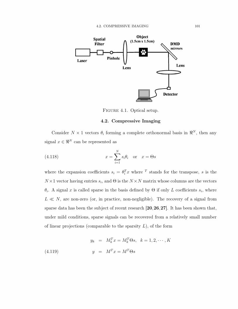
4.2. COMPRESSIVE IMAGING 101
Figure 4.1. Optical setup.
4.2. Compressive Imaging
Consider N × 1 vectors θi forming a complete orthonormal basis in �N , then any
signal x ∈ �N can be represented as
(4.118) x =
N∑i=1
siθi or x = Θs
where the expansion coefficients si = θTi x where T stands for the transpose, s is the
N×1 vector having entries si, and Θ is the N×N matrix whose columns are the vectors
θi. A signal x is called sparse in the basis defined by Θ if only L coefficients si, where
L � N , are non-zero (or, in practice, non-negligible). The recovery of a signal from
sparse data has been the subject of recent research [20,26,27]. It has been shown that,
under mild conditions, sparse signals can be recovered from a relatively small number
of linear projections (comparable to the sparsity L), of the form
yk = MTk x =MT
k Θs, k = 1, 2, · · · , K
y = MTx =MTΘs(4.119)

4.2. COMPRESSIVE IMAGING 102
where the N × 1 vectors Mk, k = 1, 2, · · · , K define the projective measurements. Ran-
dom projections, yielding incoherence between the projective measurements basis and
the sparsity basis, are ideal, giving a reduced number of experiments for the desired
signal recovery. At the heart of the reconstruction procedure is the minimization of the
1-norm, ‖s‖1, of s, which can be done readily. Many physical signals are sparse in a
known basis (wavelets, etc.), hence this approach has enormous practical importance.
Furthermore, the general 1-norm-based reconstruction approach can be extended to
a broader class of signals that become sparse under a given transformation, being of
particular interest sparse-gradient signals, characterized as follows. Let xi,j represent
the pixel in the ith row and jth column of an n× n image x, and define the operators
Dh;i,jx =
⎧⎪⎪⎨⎪⎪⎩xi+1,j − xi,j i < n
0 i = n
and
Dv;i,jx =
⎧⎪⎪⎨⎪⎪⎩xi,j+1 − xi,j j < n
0 j = n
and
Di,jx =
⎛⎝ Dh;i,jx
Dv;i,jx
⎞⎠In this way, the vector Di,jx can be considered a discrete gradient of the image x. In
sparse-gradient signals, the gradient Di,jx is sparse. This sparsity arises, e.g., in certain
piecewise constant signals. One can then define the total variation (TV) of x as
TV (x) =∑i,j
√(Dh;i,jx)2 + (Dv;i,jx)2
=∑i,j
‖Di,jx‖2(4.120)

4.3. OPTICAL SIGNAL MODEL 103
and recover the signal by solving
(4.121) min TV (x) subject to∥∥MTx− y
∥∥2≤ ε
where ε represents the noise level. This is the reconstruction approach adopted in the
following.
4.3. Optical Signal Model
Under coherent light illumination, the mapping from the field ψ0(x, y) that impinges
on the DMD to the intensity at the detector plane is of the form
(4.122) Ik(u, v)=
∣∣∣∣∫ ∫S
dxdyψ0(x, y)Mk(x, y)h(u, v; x, y)
∣∣∣∣2where S is the area of the DMD, Mk(x, y) denotes the reflectivity function of the DMD
corresponding to state k of the DMD (in the present work, a binary pattern), I(u, v)
represents the light intensity at the coordinates (u, v) in the detector plane, and h is the
impulse response of the lens from the DMD plane to the photodetector plane. Generally
h incorporates diffraction effects. In contrast, under incoherent light illumination, the
respective mapping is of the form ( [39], eq. 6.15)
(4.123) Ik(u, v)=
∫ ∫S
dxdy|ψ0(x, y)|2|Mk(x, y)h(u, v; x, y)|2
which defines the linear mapping from field intensity at the DMD to field intensity at
the detector plane. Continuing on the incoherent case, consider now a bucket detector
of capture area D, then the output signal Pk is given by
(4.124) Pk=
∫ ∫S
dxdy|ψ0(x, y)|2∫ ∫
D
dudv|Mk(x, y)h(u, v; x, y)|2

4.3. OPTICAL SIGNAL MODEL 104
which is a linear projection of the intensity |ψ0(x, y)|2 at the DMD onto M ′k(x, y) where
M ′k(x, y) =
∫ ∫D
dudv|Mk(x, y)h(u, v; x, y)|2,
as desired. Importantly, in the incoherent case this holds for any D. It is apparent
from (4.122) that this is not the case for coherent light and that only under special
circumstances the respective mapping can be dealt with as a projective measurement.
Consider, for example, the special case of a point-like, single-pixel detector at (u, v).
Then from (4.122) the output signal
(4.125) Pk � I(u, v) = |P ′k|2
where P ′k is a projective measurement (of ψ0) of the form
(4.126) P ′k=
∫ ∫S
dxdyψ0(x, y)Mk(x, y)h(u, v; x, y),
however, this is of limited use unless one uses phase retrieval or holographic measure-
ments to recover the complex field ψ0 at the DMD.
The situation assumed in this thesis is the special case of geometrical optics condi-
tions where diffraction effects are negligible. Also, the distances from the DMD to the
lens and from the lens to the detector are chosen such that the lens law of geometrical
optics holds, to ensure focusing of the DMD-reflected light at the detector. So long
as D is sufficiently large (a “bucket detector” [40,41]) to cover completely the image
plane counterpart of S (an area identical to S but lens-magnified), then in this case the
captured integrated intensity ( [39], eqs. 5.33-5.40)
(4.127) Pk=
∫ ∫D
dudvI(u, v)=
∫ ∫S
dxdy|ψ0(x, y)|2|Mk(x, y)|2
which has the desired projective measurement form. In particular, this is the same
form as equation (4.119), with the obvious substitutions x → ψ0, y → P (where P is

4.4. RESULTS AND DISCUSSION 105
the vector having entries Pk, k = 1, 2, · · · , K), and Mk → |Mk|2. Thus the discussion
in Section 2 applies to this optical model. We discuss next experimental results that
illustrate the application of compressive sensing ideas to recover images of coherent
light intensity using the combined DMD-lens-single detector system in Figure 1.
4.4. Results and Discussion
As imaging objects, we considered two apertures, one with the shape of a paw
print (symbol of Northeastern University’s mascot) and another with the shape of the
letter “T” (see Figure 4.2). For future reference, images of these objects captured with
a CCD camera positioned at the DMD plane (in place of the combined DMD-lens-
detector system of this work) are also shown in Figure 4.2. An 10.5mm×10.5mm area
of 768×768 DMD mirrors, each mirror being of 13.68μm×13.68μm (Texas Instruments’
DMD Discovery 3000 series), was used to generate the random projective measurements.
Squares of 24 × 24 adjacent mirrors acted in unison as a single effective patch in the
generation of the masks. Thus the masks were 32× 32 patch signals.
We considered two ways of capturing the data. In the first, mono-patch or “semi-
synthetic data” approach, data were captured using masks with a single patch “on”,
and subsequently due to linearity (of the field intensity to detector output map) the
corresponding data for arbitrary random masks were computed and used to create
the reconstructions. The second, multi-patch approach directly applies random 32×32
patch masks, drawn from a Bernoulli probability distribution. The two approaches gave
comparable images, but the images based on the mono-patch approach were better. The
mono-patch approach allows better control of light intensity, noise level, and diffrac-
tion and interference effects. This method also constitutes a coarse scanning imaging
system which uses much less data than a conventional CCD camera (even without the
intermediary step of mapping from raw data to semi-synthetic random mask data as
outlined above).

4.4. RESULTS AND DISCUSSION 106
(a) (b)
(c) (d)
Figure 4.2. Objects used in the experiments: a) paw print, and c) T.Figures b) and d) are 300 × 300 pixel images of “paw print” and “T”,respectively, taken with a CCD camera positioned at the DMD plane.

4.4. RESULTS AND DISCUSSION 107
Figure 4.3 (a) shows the reconstructed image of the field intensity produced at the
DMD plane by the paw print aperture (Figures 4.2 (a) and (b)), from 500 mono-patch or
semi-synthetic measurements. After filtering out what appeared to be noise-produced
outliers, we obtained a more select set of 409 such measurements, yielding the image in
Figure 4.3 (b). The results are encouraging. To compare the results of mono-patch data
with those of multi-patch data, we repeated the inversion process using the results of
random mask measurements. Figures 4.3 (c) and (d) illustrate the results with multi-
patch data, which clearly are comparable to those with mono-patch data. However, the
images from multi-patch data are more noisy than the mono-patch counterparts, which
we attribute mostly to the reduced control over light intensity, noise level and other
wave system perturbations in the multi-patch case relative to the mono-patch case. It
is important to emphasize that these images were obtained with much less data than
the CCD camera image in Figure 4.2 (b), which consists of 300 × 300 pixels (90,000
data), however they still capture the essence of the object.
To obtain results for objects with sharper edges, we replaced the paw print aperture
with the T-shaped aperture in Figures 4.2 (c) and (d), and repeated the experiment.
Again we note that using multi-patch data (390 samples) for the inversion process
(Figure 4.4 (b)) results in more noise in the resulting image than using mono-patch
data (409 samples) (Figure 4.4 (a)). To further test the reconstruction approach, and
the possibility of imaging with less data, we selected 204 apparently reliable mono-
patch samples. In this case, we were able to recover a highly recognizable image (see
Figure 4.4 (c)). While the edges are not as sharp as those in the image recovered from
the 409 mono-patch samples, the overall image is largely the same. Also note that the
204-mono-patch data image is of greater quality than the image recovered from 390
multi-patch data, even though the latter involves twice more measurements.

4.5. CONCLUSIONS 108
(a) (b)
(c) (d)
Figure 4.3. Reconstructions of the “paw print” field. a) 500 mono-patchor semi-synthetic measurements, b) 409 mono-patch measurements, c)500 multi-patch measurements, and d) 350 multi-patch measurementswith range constraints.
4.5. Conclusions
We have experimentally and computationally demonstrated a new coherent single-
detector imaging system that is based on the principles of the nascent field of compres-
sive sensing which allows data compression at the sensor level. Single-detector cameras
are among the most exciting applications of compressive sensing. However, they use
incoherent light which involves a linear object-to-data mapping even if diffraction ef-
fects are non-negligible, as we showed in Section 4.3. As shown in Section 4.3, it is not

4.5. CONCLUSIONS 109
(a) (b)
(c)
Figure 4.4. Reconstructions of the “T” field. a) corresponds to 409mono-patch or semi-synthetic samples, b) corresponds to 390 multi-patchdata, and c) corresponds to 204 mono-patch samples.
obvious that single-detector cameras can be used also for computational imaging with
coherent laser light where the mapping from object to intensity-only data is generally
nonlinear. However, we showed in this work, theoretically (in Section 4.3) and prac-
tically (in Section 4.4), that under geometrical optics conditions for which an image
casting sensor architecture applies, then the single-detector camera can also be used
for coherent single-detector imaging. For our demonstrations we adopted two different
approaches, one based on random masks (multi-patch method), and another one based

4.5. CONCLUSIONS 110
on coarsely scanned data (mono-patch approach). The latter approach functioned bet-
ter, mostly thanks to better control of light intensity, noise level, and diffraction and
coherent interference effects.
This effort is rich in future directions. In this thesis the focus has been on the
reconstruction of field intensity images. But clearly the same general approach could
be extended also to a full amplitude and phase imaging if one uses reference beams as in
holography. Furthermore, in addition to field images, if full amplitude and phase field
information is available, one can invert via compressive sensing methods the source or
object to field mapping and compute object images as in optical inverse diffraction and
tomography applications.

Bibliography
[1] F. Simonetti, M. Fleming, and E. A. Marengo, “An illustration of the role of multiple scattering
in subwavelength imaging from far-field measurements,” Journal of Opt. Soc. Am. A, vol. 25, pp.
292–303, 2008.
[2] A. Sentenac, C. Guerin, P. Chaumet, F. Drsek, H. Giovannini, N. Bertaux, and M. Holschneider,
“Influence of multiple scattering on the resolution of an imaging system: Cramer-rao analysis,”
Optics Express, vol. 15, pp. 1340–1347, 2007.
[3] X. Chen and Y. Zhong, “Influence of multiple scattering on subwavelength imaging: transverse
electric case,” Journal of Opt. Soc. Am. A, vol. 27, pp. 245–250, 2010.
[4] E. Wolf, “Three-dimensional structure determination of semi-transparent objects from holographic
data,” Optics Communications, vol. 1, pp. 153–156, Sept 1969.
[5] A. Brancaccio, G. Leone, and R. Pierri, “Information content of born scattered fields: results in
the circular cylindrical case,” Journal of Opt. Soc. Am. A, vol. 15, pp. 1909–1917, 1998.
[6] R. Pierri, R. Persico, and R. Bernini, “Information content of born field scattered by an embedded
slab: multifrequency, multiview, and multifrequency-multiview cases,” Journal of Opt. Soc. Am.
A, vol. 16, pp. 2392–2399, 1999.
[7] S. M. Kay, Fundamentals of Statistical Signal Processing: Estimation Theory. Upper Saddle
River,NJ: Prentice Hall, 1993.
[8] M. Shahram and P. Milanfar, “Imaging below the difraction limit: A statistical analysis,” IEEE
Trans. Image Processing, vol. 13, pp. 677–689, 2004.
[9] G. Shi and A. Nehorai, “Cramer-rao bound analysis on multiple scattering in multistatic poitn-
scatterer estimation,” IEEE Trans. Signal Processing, vol. 55, pp. 2840–2850, 2007.
[10] M. Cheney and R. J. Bonneau, “Imaging that exploits multiple scattering from points scatterers,”
Inverse Problems, vol. 20, pp. 1691–1711, 2004.
[11] N. Engheta and R. W. Ziolkowski, Metamaterials: Physics and Engineering Explorations. Wiley-
IEEE Press, 2006, ch. 2.
111

BIBLIOGRAPHY 112
[12] F. Chen, W. Chew, X. Yin, and W. Hong, “Study of resolution and super resolution in electro-
magnetic imaging for half-space problems,” IEEE Transactions on Antennas and Propagation,
vol. 52, no. 6, pp. 1398–1411, June 2004.
[13] ——, “Experimental verification of super resolution in nonlinear inverse scattering,” Appl. Phys.
Lett., vol. 72, pp. 3080 – 3082, 1998.
[14] K. Belkebir, P. Chaumet, and A. Sentenac, “Influence of multiple scattering on three dimensional
imaging with optical diffraction tomography,” Journal of Opt. Soc. Am. A, vol. 23, pp. 586–595,
2006.
[15] F. Simonetti, “Multiple scattering: The key to unravel the subwavelength world from the far-field
pattern of a scattered wave,” Physical Review E (Statistical, Nonlinear, and Soft Matter Physics),
vol. 73, no. 3, p. 036619, 2006.
[16] M. Zambrano, E. A. Marengo, and D. Brady, “Cramer-rao study of scattering systems in one-
dimensional space,” in IASTED International Conference on Antennas, Radar, and Wave Prop-
agation, November 2010.
[17] M. Gustafsson and S. Nordebo, “Cramer lower bounds for inverse scattering problems of multilayer
structures,” Inverse Problems, vol. 22, pp. 1359–1380, 2006.
[18] E. A. Marengo, M. Zambrano, and D. Brady, “Cramer-rao study of one-dimensional scattering
systems: Part i: Formulation,” in IASTED International Conference on Antennas, Radar, and
Wave Propagation, July 2009.
[19] ——, “Cramer-rao study of one-dimensional scattering systems: Part ii: Computer simulations,”
in IASTED International Conference on Antennas, Radar, and Wave Propagation, July 2009.
[20] E. Candès, “Compressive sampling,” in Congress of Mathematicians, vol. 3, 2006, pp. 1433–1452.
[21] D. Donoho, “Compressed sensing,” IEEE Trans. on Information Theory, vol. 52, pp. 1289–1306,
2006.
[22] R. DeVore, B. Jawerth, and B. Lucier, “Image compression through wavelet transform coding,”
IEEE Transaction on Information Theory, vol. 38, pp. 719–746, 1992.
[23] M. Antonini, M. Barlaud, P. Mathieu, and I. Daubechies, “Image coding using wavelet transform,”
IEEE Transaction on Image Processing, vol. 1, pp. 205–220, 1992.
[24] D. Takhar, J. Laska, M. Wakin, M. Duarte, D. Baron, S. Sarvotham, K. Kelly, and R. Baraniuk, “A
new compressive imaging camera architecture using optical-domain compression,” Computational
Imaging IV, vol. 6065, pp. 43–52, 2006.

BIBLIOGRAPHY 113
[25] M. Duarte, M. Davenport, D. Takhar, J. Laska, T. Sun, K. Kelly, and R. Baraniuk, “Single-pixel
imaging via compressive sampling,” IEEE Signal Processing Magazine, vol. 25, pp. 83–91, 2008.
[26] E. Candès, J. Romberg, and T. Tao, “Robust uncertainty principles: Exact signal reconstruction
from highly incomplete frequency information,” IEEE Trans. Information Theory, vol. 52, pp.
489–509, 2006.
[27] R. Baraniuk, “Compressive sensing,” IEEE Signal Processing Magazine, vol. 24, pp. 118–121, 2007.
[28] W. Chan, K. Charan, D. Takhar, K. Kelly, R. Baraniuk, and D. Mittleman, “A single-pixel
terahertz imaging system based on compressed sensing,” Appl. Phys. Lett., vol. 93, pp. 121 105–3,
2008.
[29] G. B. Arfken and H. J. Weber, Mathematical Methods For Physicists, 5th ed. San Diego, CA:
Academic Press, 2001.
[30] C. A. Balanis, Advanced Engineering Electromagnetics. Wiley, 1989.
[31] J. Shao, Mathematical Statistics, 2nd ed. New York, NY: Springer Verlag, 1999.
[32] H. V. Poor, An Introduction to Signal Detection and Estimation, 2nd ed. New York, NY: Springer
Verlag, 1994.
[33] M. Born and E. Wolf, Principles of Optics: Electromagnetic Theory of Propagation, Interference
and Diffraction of Light, 7th ed. Cambridge University Press, 1999.
[34] L. L. Scharf, Statistical Signal Processing, Detection, Estimation, and Time Series Analysis. Pear-
son Education, 2002.
[35] K.-H. D. L. Tsang, J.A. Kong and C. Ao, Scattering of Electromagnetic Waves: Numerical Sim-
ulations. New York: John Wiley & Sons, 2001.
[36] H. Lutkepol, Handbook of Matrices. New York: John Wiley, 1996.
[37] A. van de Bos, “A cramer rao lower bound for complex parameters,” IEEE Transactions on Signal
Processing, vol. 42, p. 2859, October 1994.
[38] E. A. Marengo, F. Gruber, and F. Simonetti, “Time-reversal music imaging of extended targets,”
IEEE Transactions on Image processing, vol. 16, pp. 1967–1984, 2007.
[39] J. Goodman, Ghost imaging with a single detector, 3rd ed. Greenwood Village,CO: Roberts &
Company, 2005.
[40] Y. Bromberg, O. Katz, and Y. Silberbergi, “Ghost imaging with a single detecto,” Physical Review
A, vol. 79, pp. 053 840–4, 2009.

BIBLIOGRAPHY 114
[41] O. Katz, Y. Bromberg, and Y. Silberbergi, “Compressive ghost imaging,” Appl. Phys. Lett, vol. 95,
pp. 131 110–3, 2009.