Statistical Signal Processing - 大阪工業大学 ...kamejima/lectureNotes/SSslide.pdf ·...
147
Statistical Signal Processing An Experimental Mathematics Approach ∗ Kohji Kamejima † December 22, 2009 ∗ † Faculty of Information Science and Technology, Osaka Institute of Technology
Transcript of Statistical Signal Processing - 大阪工業大学 ...kamejima/lectureNotes/SSslide.pdf ·...

Statistical Signal Processing
An Experimental Mathematics Approach∗
Kohji Kamejima†
December 22, 2009
∗†Faculty of Information Science and Technology, Osaka Institute of Technology

2
Linux

3
1 Random Numbers 1
1November 17

4
GPS User Segment: Personal Navigator

5
GPS User Segment: Statistical Analysis

6
SRV Rendezvous
IMGraph.c[img]

7
SRV Network Integration
Vehicle Segment
Relay Site
pseudo range
longitude-latitude
Roadway Segment
Satellite Image

8
SRV Tracking Signal
GGLLT.c[ggllt]

9
GPS: Fluctuation

10
GPS: Bias

11
GPS: Model Error

12
Getting Software Package
First of all create a folder entitled by ISS under properly chosen main folder, say Cprograms.

13
Getting Software Package
Visit http://www.is.oit.ac.jp/~kamejima/ to download ISS.tar UNIX archive file into ISS.
Extract all files into ISS folder.
All the utility functions are stored in initXWindow.h. Please download it into Cprogramsfolder so that the initXWindow.h file should be included via #include ‘‘../initXWindow.h’’command.
Use PR.c program for the simulation associated with probability and statistics.
Use AR.c program for simulating autoregression model.
The KF.c program can be utilized as the basis for designing filter dymanics.
In the GPS package you can find C programs and toolkit for analyzing GPS signals and relatedionosphere processes.

14
Random Numbers: rand()
Random Number Generator
rt+1 ← (k · rt + c) mod m, (1a)r0 ∈ Z, (1b)
k = 1103515245,
c = 12345,
m = 32768.
mod : modulo operator

15
Coin Game: HT.c
Mathematician Trials FrequencyBuffon 4040 0.507
de Morgan 4092 0.5005Jevons, S. (Economist) 20480 0.5068
Romanovsky 80640 0.4923Pilson 24000 0.5009Feller 10000 0.4947
Program: PRrandomB(double probability )

16
Coin Game (HT.c)#include "./initPR.h"int main(int argc, char *argv[]){....................while(True){....................// Coin Game ..... startstrcpy(text, "T");if(rand()%2==0){strcpy(text, "H");sumH++;
} else {strcpy(text, "T");sumT++;
}// Coin Game ..... end....................}// end of time loopprintf(" End of HT. ButtonPress for Exit, please\n");
}

17
Coin Game (CoinGame.c)CoinGame(int length, int mask, int* ptrEvent, double* ptrValue){....................int Hgain=1;int Tgain=-1;int Event=0;int Gain=0;for(i=0; i<length; i++){....................Rnumber = rand()%2;....................Event = 2*Event + Rnumber;if(Rnumber>0) Gain += Hgain;if(Rnumber<=0) Gain += Tgain;
}....................return (mask & Event)==mask;
}
x(H) Hgainx(T) Tgain∑t
xt Gain
H-T pattern Eventcondition (H***,HH**,. . . ) mask

18
Accident: PR.c, PRdistribution.c
• HH, HHH, HHHH,. . .
Year Total Letters No Address Frequency(×10−6)
1906 983,000,000 26,112 26.561907 1,076,000,000 26,977 25.071908 1,214,000,000 33,515 27.611909 1,357,000,000 33,643 24.701910 1,507,000,000 40,101 26.61
Program: PRrandomBS(int N, double probability )

19
Buffon’s Needles: BF.c, Buffon.c
P =2`
πa (` ≤ a)
Program: Buffon, BuffonNeedle

20
Buffon’s Needles: BF.c, Buffon.c
a
x
0
θ
`
y =x
cos θ
y
P (0 ≤ y ≤ `) =∫ π/2
0
P (0 ≤ x ≤ a | θ)(
dθ
π/2
)=
∫ π/2
0
(min { ` cos θ, a }
a
)(dθ
π/2
)
=
2`
πa
∫ π/2
0
cos θdθ; for ` ≤ a,
???; otherwise.
Program: Buffon, BuffonNeedle

21
Buffon’s Needle (BF.c)#define BUFFON_A 100#define BUFFON_L 50....................// Time LoopSamples = 0; Matches = 0;while(WaitGoExit(&BFW)){Samples++;Condition = BuffonNeedle(BFW, BUFFON_A, BUFFON_L);if(Condition) Matches++;// Statistical Momentssprintf(text, "%4.1f%(%d/%d)",100*(double)Matches/Samples, Matches, Samples);BoxedString(BFW, 0, 10, text, BLUE, WHITE);//getchar();....................}// end of loop....................

22
Buffon’s Needle(Buffon.c)Buffon(double* ptrPoint, int Abuffon, int Lbuffon){double Rshift=Abuffon*Random01();double Rtheta=(PI/2)*Random01();double x=Lbuffon*cos(Rtheta)-Rshift;int cross=(x>=0);double point=0;if((Rtheta<(PI/2))&&(cross))point = x/cos(Rtheta);
....................return cross;
}a
x
0
θ
`
y =x
cos θ
y
a Abuffon` Lbuffonx Rshiftθ Rthetay cross
` cos θ − x x

23
Two Approaches
24
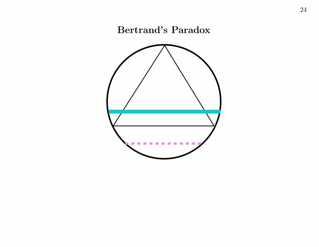
Bertrand’s Paradox

25
Bertrand’s Paradox
Model-1: P =12
Model-2: P =13
Model-4: P = 0Model-3: P =
14

26
Gaussian Process
200 400 t
−1
w
1
Program: PRrandomG()

27
Gaussian Distribution: PR.c, PRdistribution.c
Program the following generator of Gaussian random numbers {wt, t = 0, 1, 2, . . . }based on rt.
wt =
{√Gt; for Gt ≥ 0,
−√
Gt; otherwise,(1a)
Gt = yt
[a0 +
a1
yt + a2
], (1b)
a0 = 2.0611786, a1 = −5.7262204, a2 = 11.640595,
yt = − log[(1 + rt)(1 − rt)]. (1c)
Statistics of random numbers can be designed via “histogram equalization.” Sam-ple values at each iteration time (·) are scattered around “mean value (=0)” with“variance (=1)”.
Program: PRInvGauss(double xpm)

28
Gaussian Distribution: PR.c, PRdistribution.c
P (|y| ≤ σ) ' 0.6826P (|y| ≤ 2σ) ' 0.9545P (|y| ≤ 3σ) ' 0.9973
−5 0y
5
0.5
√2πp
1
Program: PRrandomGcLt(int n)

29
Central Limit Theorem
Program the generator of random numbers given by
yn =r1 + r2 + r3 + · · · + rn√
σ · n. (1)
The histogram of finite sum of independent random numbers converges to the Gauss-ian distribution.

30
Random Number (PR.c)#define BUFFON_A 10#define BUFFON_L 4#define CG_LENGTH 16#define CG_MASK 0x0000 //0x0000 0x8000 0xc000 0xe000 0xf000....................int main(int argc, char *argv[]){....................// Time Loop
....................// Random Numbersvalue = 0.05*PRrandomBpmS(1000, 0.5);dp=0.1*dp0;Condition = CoinGame(Clength, Cmask, &Event, &value);dp=0.01*dp0;Condition = Buffon(&value, ...);dp=dp0;// end of Random Numbers
....................}

31
Random Number (RN.c)RNsample(double* ptrValue){int Mlevel=3, Condition=True;double value=*ptrValue;value = RandomGx2(10);value = RandomGcLt(10);value = 1*RandomG()+0;value = 1*RandomU()+0;value = RandomBpm(0.5);//value = RandomT(10*DT/T_MAX);//value = 0.1*RANDOM_TIME;//value = 4*DT*Casino(0.51, BANKRUPTCHY_SUM);//if(fabs(value)>Mlevel) Condition = True;*ptrValue = value;return Condition;
}
Binary Distribution RandomBpm( probability )Uniform Distribution RandomU()
Gaussian Distribution RandomG() (Central Limit Theorem: RandomGclt( n ))χ2 Distribution RandomGx2( n )

32
2 Stochastic Differential Equation – finite differencescheme – 2
2November 24

33
Simulation Physics: Galilei’s World
GL.c/’G’[gl]

34
Getting Software Package
Create DE folder in Cprograms.

35
Getting Software Package
Visit http://www.is.oit.ac.jp/~kamejima to download DE.tar UNIX archive file into DE.
Extract all files into DE folder.
Use GL.c program for simulating Galilei-Aristotle World.
Use DE1.c program for the simulation of first order system.
Use DE2.c program for simulating second order system.
The DE.c program can be utilized as mathematical model of dynamicsl systems.

36
Simulation Physics: Aristotle’s World
GL.c/’A’[gl]

37
Simulation Physics (GL.c)#define GRV -9.8#define GA_MODE ’G’ // ’A’ // Galilei -- Aristotle....................int main(int argc, char *argv[]){
....................while(WaitGoExit(&(GLgraph.wi))){Galilei(GLgraph, GA_MODE, g, t, y, &dydt, dt); //Galilei-Aristotle....................
}// end of t-loop....................return True;
}....................

38
Newton’s World
f = ma, (1)f = −mg, g = 9.8m/s2 (2)
Position : y(t), (3)
Velocity : v(t) =dy(t)dt
, (4)
Acceleration : a =dv(t)dt
=d
dt
(dy(t)dt
)=
d2y(t)dt2
. (5)
Differential Equation : −g = a =d2y(t)dt2
. (6)
Finite Difference :dy
dt∼ y(t + dt) − y(t)
dt, (7)
d2y
dt2∼
dy(t + dt)dt
− y(t)dt
dt. (8)

39
Newton’s World – Simulated
Differential Equation : −g = a =d2y(t)dt2
. (1)
Finite Difference :dy
dt∼ y(t + dt) − y(t)
dt, (2)
d2y
dt2∼
dy(t + dt)dt
− y(t)dt
dt, (3)
Forward Difference : y(t + dt) ∼ y(t) +dy
dtdt, (4)
dy(t + dt)dt
∼ y(t)dt
− gdt, (5)
Programming : y ← y + dydt*dt, (6)dydt ← dydt− g*dt, (7)

40
Simulation Physics (initDE.h)
int Galilei(struct XGRAPH_INFO GR, char mode, double g,double t, double y, double* ptrDydt, double dt)
{double d2ydt2=g;double dydt=*ptrDydt;int radius=5;if(mode==’G’){// Galilei-Newtonif(y<0) d2ydt2 = -2*dydt/dt;dydt += d2ydt2*dt;
}if(mode==’A’){// Aristotleif(y>=Y0) dydt = g;if(y<=0) dydt = -g;
}DrawGraphCircle(GR, t, y, radius, GREEN, WHITE);
....................}

41
2.1 First Order System

42
Dynamical Systems: DE1.c

43
Dynamical Systems: DE1.c
αγ
β
isotope [C14]

44
Differential Equation: First Order System
Differential Equation:
dx(t)
dt= f [x(t)], x(0) = x0.
Simple Example:
dx(t)
dt= −ax(t), x(0) = x0.
Solution:
x(t) = x(0) exp [−at] ,( dx
x= −adt
)

45
Differential Equation: Forward Difference
Differential Equation:
dx(t)
dt= f [x(t)], x(0) = x0.
Integral Representation:
x(t) = x0 +
∫ t
0
f [x(s)]ds.
Forward Difference:
x(dt) = x(0) +
∫ dt
0
f [x(s)]ds ' x(0) + f [x(0)]dt.
x(t + dt) ' x(t) + f [x(t)]dt.

46
Dynamical Systems: DE1.c

47
Differential Equation: DE1.c -- MainLoop
#define Y0 1.............................int main(int argc, char *argv[]){.............................// t-Loopt = T0;y = Y0;while(WaitGoExit(&(DEgraph.wi))){// Input ... startf = 0;// Input ... end.............................// Differential Equation ... start// First Order Equation.............................dydt = -0.2*y;// Differential Equation ... end.............................
}// end of t-loop}

48
Differential Equation: DE1.c -- Plot
#define Y0 1.............................int main(int argc, char *argv[]){.............................// t-Loopt = T0;y = Y0;while(WaitGoExit(&(DEgraph.wi))){.............................DrawGraphPoint(DEgraph, h, y, GREEN);DrawGraphPoint(DEgraph, h, f, BLUE);.............................
}// end of t-loop}

49
Differential Equation: DE1.c -- Update
#define Y0 1.............................int main(int argc, char *argv[]){.............................while(WaitGoExit(&(DEgraph.wi))){.............................// Dynamicsl Systemdydt += f;// Dynamicsl System ... end// Forward Differencey += dydt*dt;.............................
}// end of t-loop}

50
Dynamical Systems: DE1.c

51
Differential Equation: DE1.c -- Excitation
#define Y0 0.............................int main(int argc, char *argv[]){.............................while(WaitGoExit(&(DEgraph.wi))){// Input ... startf = 0;//f = 1*sin(20*t)+0;// Input ... end.............................
}// end of t-loop}

52
2.2 Second Order System

53
Dynamical Systems: DE2.c

54
Differential Equation: Second Order System
Differential Equation:
d2y
dt2+ 2ζωn
dy
dt+ ω2
ny = 0, y(0) = y0,dy(0)
dt= y0.
(x1, x2): x1 = y, x2 =dy
dt..
dx1
dt= x2,
dx2
dt=
d2y(t)
dt2= −2ζωn
dy
dt− ω2
ny
= −2ζωnx2 − ω2nx1.
Programming:
x1 : y ← y + dydt*dt,
x2 : dydt ← dydt + d2ydt2+dt,
d2ydt2 = −2ζωny*dt− ω2nx*dt.

55
Differential Equation: DE2.c -- MainLoop
#define Y0 1#define DY0 0.............................int main(int argc, char *argv[]){.............................while(WaitGoExit(&(DEgraph.wi))){
.............................// Input ... startf = 0;// Input ... end.............................// Differential Equation ... start// Second Order Equation.............................d2ydt2 = -2*dydt - 2*y;d2ydt2 = -3*dydt -2*y;.............................// Differential Equation ... end.............................}// end of t-loop
.............................}

56
Differential Equation: DE2.c -- Update
#define Y0 1#define DY0 0.............................int main(int argc, char *argv[]){.............................while(WaitGoExit(&(DEgraph.wi))){// Second Order Systemd2ydt2 += f;// Second Order System ... end// Forward Differencedydt += d2ydt2*dt;y += dydt*dt;.............................}// end of t-loop
.............................}

57
Dynamical Systems: DE2.c

58
Differential Equation: DE2.c -- Excitation
#define Y0 0 // 1#define DY0 0.............................int main(int argc, char *argv[]){.............................while(WaitGoExit(&(DEgraph.wi))){
.............................// Input ... startf = 0;//f = 1*sin(1*t)+0;// Input ... end.............................}// end of t-loop
.............................}

59
Differential Equation: Second Order System
Differential Equation:
d2y
dt2+ 2ζωn
dy
dt+ ω2
ny = 0, y(0) = y0,dy(0)
dt= y0.
Vector Form:
x1 = y, x2 =dy
dt.
d
dt
[x1
x2
]=
dx1
dtdx2
dt
=
[x2
−2ζωnx2 − ω2nx1
]=
[0 1
−ω2n −2ζωn
] [x1
x2
]
First Order System:
dx
dt= Ax, x =
[x1
x2
], A =
[0 1
−ω2n −2ζωn
].

60
Differential Equation: DE.c -- MainLoop
#define X0 0 // 0.5#define Y0 0 // 0.5.............................int main(int argc, char *argv[]){.............................while(WaitGoExit(&(DEgraph.wi))){.............................// Input ... startf = 0;g = 0;// Input ... end// Differential Equation ... start// System.............................dxdt = y;dydt = -2*x -2*y + 3;.............................// Differential Equation ... end.............................
}// end of t-loop.............................}

61
Differential Equation: DE.c -- Plot
#define X0 0 // 0.5#define Y0 0 // 0.5.............................int main(int argc, char *argv[]){.............................// t-Loopt = T0;x = X0;y = Y0;while(WaitGoExit(&(DEgraph.wi))){.............................DrawGraphPoint(DEgraph, h, x, RED);DrawGraphPoint(DEgraph, h, y, GREEN);.............................
}// end of t-loop.............................}

62
Differential Equation: DE.c -- Update
#define X0 0 // 0.5#define Y0 0 // 0.5.............................int main(int argc, char *argv[]){.............................while(WaitGoExit(&(DEgraph.wi))){.............................// Forward Differencex += dxdt*dt + f*dt;y += dydt*dt + g*dt;.............................
}// end of t-loop.............................}

63
2.3 Stochastic Differential Equation

64
Dynamical Systems: DE2.c

65
Stochastic Differential Equation
Differential Equation:
dx(t)
dt= f [x(t)] + Gn(t), x(0) = 0,
E{n(t) } = 0, E{n2(t) } = 1.
Integral Representation:
x(t) =
∫ t
0
f [x(s)]ds +
∫ t
0
Gn(s)ds.
Forward Difference:
dx ' f [x]dt + Gndt.

66
Stochastic Differential Equation: White Noise
Formal Representation:
dx = f [x]dt + Gndt,
E{n(t) } = 0, E{n2(t) } = 1.
Brownian Motion:
ndt ∼ σdw,
E{ dw } = 0, E{ dw2 } = dt
σ2E{ dw2 } = σ2dt ∼ E{n2dt2 } = dt2,
σ2 ∼ dt.
n ∼ σdw
dt=
√dt
dw
dt.

67
Stochastic Differential Equation: White Noise
MAthematical Representation:
dx = f [x]dt + Gdw,
E{ dw } = 0, E{ dw2 } = dt.
Equivalent Representation:
dw
dt∼ n√
dt.
dx
dt= f [x] +
G√dt
n.

68
Differential Equation: DE1.c
#define Y0 1.............................int main(int argc, char *argv[]){.............................while(WaitGoExit(&(DEgraph.wi))){// Input ... startf = 0;f = 0.1*RandomG()/sqrt(dt)+0;//f = 1*sin(20*t)+0;// Input ... end.............................
}// end of t-loop}

69
Differential Equation: DE2.c
#define Y0 1#define DY0 0.............................int main(int argc, char *argv[]){.............................while(WaitGoExit(&(DEgraph.wi))){
.............................// Input ... startf = 0;f = 1*RandomG()/sqrt(dt)+0;//f = 1*sin(1*t)+0;// Input ... end.............................}// end of t-loop
.............................}

70
3 Linear Stochastic Systems – from random sequence tosignals – 3
3December 1

71
Linear Stochastic System: AR Model
AR.c[issar]

72
Random Variable (RV.c)int main(int argc, char *argv[]).............................// Time Loop
.............................// Random Numbers.............................value = 0.01*PRCasino(0.51, PR_BANKRUPTCHY_SUM);value = 0.01*PRrandomL(0.01);value = PRrandomT(0.0001);value = 0.5*PR_RANDOM_TIME;value = 0.1*PRrandomBS(1000, 0.001);dp=0.02*dp0;value = 0.05*PRrandomBpmS(1000, 0.5);dp=0.3*dp0;.............................// end of Random Numbers
.............................}
Sum of Binary Random Variable PRrandomBpmS( n, probability )Number of Accidents PRrandomBS( n, probability )
Random Arrival PR RANDOM TIMERandom Jump PRrandomT( probability )Life of System PRrandomL( probability )
Life of Bank PRCasino( probability, assets )

73
Stochastic Process: AR.c
#define DT 0.001#include "./initAR.h"................................intmain(int argc, char *argv[]){//FitISSwindows();AR_DISTURBANCE=False;AR_PARAMETER=False;AR_ESTIMATE_B=False, AR_ESTIMATE_T=False, AR_ESTIMATE_M=False;AR_ERROR=False;return ARmodel();
}

74
Stochastic Process
t
x

75
Stochastic Process
Program stochastic dynamical system governed by
xt+1 = axt + wt, (1)
where {wt, t = 0, 1, 2, . . . } are Gaussian random numbers. Current state is deter-mined by current disturbance and past state. This implies that the effect of randomexcitations is fedback as future disturbances. As the result, stochastic system gen-erates complex signal ( ).
Continuous Systems:
dx
dt= αxt + wt. (2)

76
ARmodel: AR.c
ARmodel.c:
while(t<=t max){
disturbance = w(beta);
signal = x(signal, disturbance);
estimate = My a(signal);
t += dt;}
AR.c:
double My a(double x1){return 0;}int main(int argc, char *argv[]){return ARmodel();}
double w(double Bt){return Bt*sqrt(DT)*RandomG();}
double x(double x0, double w){double dxdt = alpha*x0 + w;return (1+alpha*DT)*x0 + w*sqrt(DT);}
initAR.h:
double ab(double x1);
double at(double x1);

77
Stochastic Process: ARmodel.c
double alpha=-0.05;double beta=50;double x(double x0, double w){double dxdt = alpha*x0 + w;return (1+alpha*DT)*x0 + w*sqrt(DT);
}
double w(double Bt){return Bt*sqrt(DT)*RandomG();
}
xt x( xt−dt, w )α alpha (a ∼ 1 + αdt)dt DTwt w( intensity )
Gaussian Random Number RandomG()

78
Stochastic Process: ARmodel.c
intARmodel(){double t=0, dt=DT;double signal=2, disturbance=0;double estimate=0, error=0;...........................// Time Loopwhile((t<=t_max)&&(WaitGoExitT(1000, &(Sgraph.wi)))){disturbance = w(beta);if(!AR_DISTURBANCE) disturbance = 0;signal = x(signal, disturbance);if(AR_ESTIMATE_B) estimate = ab(signal);if(AR_ESTIMATE_T) estimate = at(signal);if(AR_ESTIMATE_M) estimate = My_a(signal);error = 1000*(estimate-parameter)/parameter;.........................................// next tt += dt;
}// end of time loop..................................}

79
Stochastic Process: ARmodel.c
intARmodel(){...........................// Time Loopwhile((t<=t_max)&&(WaitGoExitT(1000, &(Sgraph.wi)))){.....................................DrawGraphPoint(Sgraph, t, signal, BLUE);if(AR_PARAMETER) DrawGraphPoint(Sgraph, t, parameter, ADRIATIC_SEA);if(AR_DISTURBANCE) DrawGraphPoint(Sgraph, t, disturbance, RED);if((AR_ESTIMATE_B)||(AR_ESTIMATE_T)||(AR_ESTIMATE_M))DrawGraphPoint(Sgraph, t, estimate, GREEN);
if(AR_ERROR) DrawGraphPoint(Sgraph, t, error, WHITE);.....................................
}// end of time loop..................................}

80
4 Parameter Estimation 4
4December 8

81
Parameter Estimation: AR Model
AR.c[issar]

82
Parameter Estimation ProblemFor linear system,
xt+1 = axt + wt,
minimize square sum of equation errors with respect to the parameter a, i.e.,
xt+1 ' axt =⇒ e2t =
t∑s=0
|xs+1 − axs|2 → min . w.r.t. a. (1)
ytxt−1
wt
axt−1

83
Parameter Estimation: Least Squares
Normal Equation:
∂e2t
∂a= 0 =⇒
t∑s=0
xs+1xs − a
t∑s=0
x2s = 0. (1)
ytxt−1
wt
axt−1

84
Parameter Estimation: AR.c
ARmodel.c:
while(t<=t max){
disturbance = w(beta);
signal = x(signal, disturbance);
estimate = My a(signal);
t += dt;}
AR.c:
double My a(double x1){return 0;}int main(int argc, char *argv[]){return ARmodel();}
double w(double Bt){return Bt*sqrt(DT)*RandomG();}
double x(double x0, double w){double dxdt = alpha*x0 + w;return (1+alpha*DT)*x0 + w*sqrt(DT);}
initAR.h:
double ab(double x1);
double at(double x1);

85
Parameter Estimator: AR.c
................................double My_a(double x1){return 0;
}................................intmain(int argc, char *argv[]){................................AR_ESTIMATE_B=False, AR_ESTIMATE_T=False, AR_ESTIMATE_M=False;................................return ARmodel();
}

86
Impulse Response
Stationary Stochastic System:
dx
dt= −ax + wt,
xt = e−atx0 + Φ(t),
Φ(t) =
∫ t
0
e−a(t−s)w(s)ds.
Steady State:
xt → Φ(t), (t → ∞)
Discrete Model: t = n · dt
Φ(t) =
t/dt∑k=0
φkw(t − kdt),
φk = e−akdt =(e−adt
)k.

87
Parameter Estimation: Successive SchemeThe least squares estimate of the linear system
xs+1 = axs + ws, s = 0, 1, 2, . . . , t
is generated by the following dynamical system:
at = at−1 + P (t)xt[xt+1 − at−1xt],
where P (t) is computed successively as follows:
P (t) = [1 + x2t P (t − 1)]
−1P (t − 1).
yt − yt
yt = at−1xt−1at−1
at

88
Recursive Algorithm
t
pax
axp

89
Stochastic Process: AR.c
#define DT 0.001#include "./initAR.h"................................intmain(int argc, char *argv[]){//FitISSwindows();AR_DISTURBANCE=True;AR_PARAMETER=True;AR_ESTIMATE_B=True, AR_ESTIMATE_T=False, AR_ESTIMATE_M=False;AR_ERROR=True;return ARmodel();
}

90
Stochastic Process: ARmodel.c
intARmodel(){double t=0, dt=DT;double signal=2, disturbance=0;double estimate=0, error=0;...........................// Time Loopwhile((t<=t_max)&&(WaitGoExitT(1000, &(Sgraph.wi)))){disturbance = w(beta);if(!AR_DISTURBANCE) disturbance = 0;signal = x(signal, disturbance);if(AR_ESTIMATE_B) estimate = ab(signal);if(AR_ESTIMATE_T) estimate = at(signal);if(AR_ESTIMATE_M) estimate = My_a(signal);error = 1000*(estimate-parameter)/parameter;.........................................// next tt += dt;
}// end of time loop..................................}

91
Stochastic Process: ARmodel.c
intARmodel(){...........................// Time Loopwhile((t<=t_max)&&(WaitGoExitT(1000, &(Sgraph.wi)))){.....................................DrawGraphPoint(Sgraph, t, signal, BLUE);if(AR_PARAMETER) DrawGraphPoint(Sgraph, t, parameter, ADRIATIC_SEA);if(AR_DISTURBANCE) DrawGraphPoint(Sgraph, t, disturbance, RED);if((AR_ESTIMATE_B)||(AR_ESTIMATE_T)||(AR_ESTIMATE_M))DrawGraphPoint(Sgraph, t, estimate, GREEN);
if(AR_ERROR) DrawGraphPoint(Sgraph, t, error, WHITE);.....................................
}// end of time loop..................................}

92
Stochastic Process: ARmodel.c
double alpha=-0.05;double beta=50;double x(double x0, double w){double dxdt = alpha*x0 + w;return (1+alpha*DT)*x0 + w*sqrt(DT);
}
double w(double Bt){return Bt*sqrt(DT)*RandomG();
}

93
Parameter Estimator: AR.c
#define DT 0.001#include "./initAR.h"
double My_a(double x1){return 0;
}
intmain(int argc, char *argv[]){..............................AR_ESTIMATE_B=False, AR_ESTIMATE_T=False, AR_ESTIMATE_M=True;..............................
}

94
Parameter Estimator: initAR.h
double x0=0;double S00=0;double S10=0;double ab(double x1){double a1=0;S00 += x0*x0;S10 += x1*x0;x0 = x1;if(S00>0) a1 = S10/S00;return a1;
}

95
Recursive Algorithm: initAR.h
double p0=100;double a0=0;double at(double x1){double p1=p0/(1+x0*x0*p0);double e1=x1-a0*x0;double a1=a0+p1*x0*e1;x0 = x1;a0 = a1;p0 = p1;return a1;
}

96
Parameter Estimation: Stochastic ApproximationThe linear system
xt+1 = axt + wt,
can be identified via the following scheme:
at = at−1 + Ktxt[xt+1 − xt+1],
xt+1 = at−1xt,
where Kt is properly designed gain.
yt − yt
yt = at−1xt−1at−1
at

97
5 Kalman Filtering 5
5December 15

98
Kalman Filter
KF.c[isskf]

99
Parameter Estimation: Successive SchemeThe least squares estimate of the linear system
xt+1 = axt + wt,
is generated by the following dynamical system:
at = at−1 + P (t)xt[xt+1 − at−1xt].
where P (t) is update gain.
yt − yt
yt = at−1xt−1at−1
at
Problem: How to generate the prediction of stochastic process xt?

100
Kalman Filter
t
pxyx
· yt
xt
xp

101
Kalman Filter (Continuous Time Model)
Stochastic System: Lsystem/initKF.h
dxt
dt= axt + wt, (1a)
yt = hxt + vt. (1b)
Filter Dynamics: KFdynamics/initKF.h
dxt
dt= axt + kt[yt − hxt], (2)
Filter Gain: KFgain/initKF.h
kt = pthσ−1vv , (3)
Error Covariance: KFcovariance/initKF.h
dpt
dt= 2apt + σww − h2p2
t σ−1vv . (4)

102
Kalman Filter (Discrete Time Model)
Stochastic System
xt+1 = axt + wt, (1a)
yt+1 = hxt+1 + vt+1. (1b)
Filter Dynamics:
xt+1 = axt + kt+1[yt+1 − hxx+1], (2a)
Filter Gain:
kt+1 = qth[h2qt + σvv]−1
, (2b)
Error Covariance:
qt+1 = a2pt + σww, pt+1 = [1 − kt+1h]qt+1.

103
Kalman Filter (Stationary Filter)
System with Observation Channel:
dxt
dt= axt + wt, (1a)
yt = hxt + vt. (1b)
Filter Dynamics:
dxt
dt= axt + k∞[yt − hxt], (2)
Stationary Gain:
k∞ = p∞hσ−1vv , (const.)(
dpt
dt→
)0 = 2ap∞ + σww − h2p2
∞σ−1vv .

104
MyFilter (a)
Stochastic System: Lsystem/initKF.h
dxt
dt= axt + wt, (1a)
yt = hxt + vt. (1b)
Filter Dynamics: MyKFdynamics/KF.c⇐ KFdynamics/initKF.h
dxt
dt= axt + kt[yt − hxt], (2)
Filter Gain: KFgain/initKF.h
kt = pthσ−1vv , (3)
Error Covariance: KFcovariance/initKF.h
dpt
dt= 2apt + σww − h2p2
t σ−1vv . (4)

105
Kalman Filter: KF.c
KalmanFilter.c:
disturbance = w(Gt);noise = v(Rt);
Lsystem(disturbance, &signal, noise, &data);
Kt=MyKFgain(pt);
estimate = MyKFdynamics(estimate, Kt, data);
pt = KFcovariance(pt);
KF.c:
double MyKFgain(double p0)
double MyKFdynamics(...)
int main(int argc, char *argv[]){return KalmanFilter();}
initKF.h:
double w(double Gt)double v(double Rt)
double KFcovariance(double p0)
double KFgain(double p0)
double KFdynamics(...)
int Lsystem(...)

106
MyFilter (b)
Stochastic System: Lsystem/initKF.h
dxt
dt= axt + wt, (1a)
yt = hxt + vt. (1b)
Filter Dynamics: MyKFdynamics/KF.c⇐ KFdynamics/initKF.h
dxt
dt= axt + kt[yt − hxt], (2)
Filter Gain: MyKFgain/KF.c
kt = k∞. (3)

107
Filter Gain: KF.c
KalmanFilter.c:
disturbance = w(Gt);noise = v(Rt);
Lsystem(disturbance, &signal, noise, &data);
Kt=MyKFgain(pt);estimate = MyKFdynamics(estimate, Kt, data);
pt = KFcovariance(pt);
KF.c:
double MyKFgain(double p0)double MyKFdynamics(...)
int main(int argc, char *argv[]){return KalmanFilter();}
initKF.h:
double w(double Gt)double v(double Rt)
double KFcovariance(double p0)
double KFgain(double p0)
double KFdynamics(...)
int Lsystem(...)

108
Stochastic System: KF.c
#define DT 0.001#define At0 -0.001#define Gt0 5.0#define Ht0 1.0#define Rt0 10.0..................int main(int argc, char *argv[]){..................//KF_L_SYSTEM=False;KF_LV_SYSTEM=True; // default: True/FalseKF_DISTURBANCE=False; // default: TrueKF_NOISE=False; // default: TrueKF_SIGNAL=True; // default: FalseKF_DATA=True; // default: TrueKF_ESTIMATE=False; // default: True//KF_MY_ESTIMATE=True;// default: Falsereturn KalmanFilter();
}

109
Stochastic System: KalmanFilter.c
int KalmanFilter(){double t=0, dt=DT;....................................// Time Loopwhile((t<=t_max)&&(WaitGoExitT(1000, &(Sgraph.wi)))){TIME = t;disturbance = w(Gt);if(!KF_DISTURBANCE) disturbance=0;noise = v(Rt);if(!KF_NOISE) noise=0;if(KF_L_SYSTEM) Lsystem(disturbance, &signal, noise, &data);if(KF_LV_SYSTEM) LVsystem(disturbance, &signal, noise, &data);................................................// next tt += dt;
}// end of time loop................................................
}

110
Stochastic System: KalmanFilter.c
int KalmanFilter(){double t=0, dt=DT;....................................// Time Loopwhile((t<=t_max)&&(WaitGoExitT(1000, &(Sgraph.wi)))){................................................Kt = KFgain(pt);if(KF_MY_GAIN) Kt=MyKFgain(pt);if(!KF_GAIN) Kt=0;estimate = KFdynamics(estimate, Kt, data);if(KF_MY_ESTIMATE) estimate=MyKFdynamics(estimate, Kt, data);pt = KFcovariance(pt);................................................// next tt += dt;
}// end of time loop................................................
}

111
Stochastic System: KalmanFilter.c
int KalmanFilter(){double t=0, dt=DT;....................................// Time Loopwhile((t<=t_max)&&(WaitGoExitT(1000, &(Sgraph.wi)))){................................................if(KF_SIGNAL) DrawGraphPoint(Sgraph, t, signal, WHITE);if(KF_DATA) DrawGraphPoint(Sgraph, t, data, CLEAR_SKY);if(KF_PT) DrawGraphPointP(Sgraph, t, pt*Pscale, RED);if(KF_ESTIMATE) DrawGraphPoint(Sgraph, t, estimate, GREEN);if(KF_MY_ESTIMATE) DrawGraphPoint(Sgraph, t, estimate, EMERALD_GREEN);................................................UpdateISShistogram(&Dhistogram,disturbance, dp, ’p’, WHITE, BLACK);UpdateISShistogram(&Nhistogram, noise, dp, ’p’, WHITE, BLACK);................................................
}// end of time loop................................................
}

112
Linear Stochastic System: initKF.h
////////////////////////////////////// Linear System//intLsystem(double Gwt, double* xt, double Rvt, double* yt){double dxdt = At*(*xt) + Gwt/sqrt(DT);Gt = Gt0;*xt += dxdt*DT;*yt = Ht*(*xt) + Rvt/sqrt(DT);return True;
}//// end of Lsystem////////////////////////////////////

113
Kalman Filter: initKF.h
double w(double Gt){return Gt*sqrt(DT)*RandomG();
}double v(double Rt){return Rt*sqrt(DT)*RandomG();
}double KFcovariance(double p0){double dpdt = 2*At*p0 + Gt*Gt - p0*Ht*(1/(Rt*Rt))*Ht*p0;return p0 + dpdt*DT;
}double KFgain(double p0){return p0*Ht/(Rt*Rt);
}double KFdynamics(double e0, double Kt, double y){double n=y-Ht*e0;double dedt = At*e0 + Kt*n;return e0 + dedt*DT;
}

114
6 Joint Paramter and State Estimation6
6December 15

115
Ionosphere Instability
Thunder Cloud
n+
e− e−
e− e− e−
e− e−e−
e−
300KV
+
-
+ n+ n- + Electrosphere
Solar RadiationSolar Wind
Cosmic Ray
Kennelly-Heaviside Layer
5780K
He++
1.4KW/m2
n+e−
450Km/s
Rn
Earth
+-

116
Whistler Effect
ISD.c[isd]

117
GPS Deviation: Longitude

118
GPS Deviation: Latitude

119
GPS: Bias

120
Linear System Model
Random Constant:
et = c + vt. (1)
Stochastic System: Lsystem/initKF.h
dxt
dt= wt, (2a)
yt = hxt + vt. (2b)

121
Kalman Filter (Continuous Time Model)
dxt
dt= kt[yt − hxt], (1)
Filter Gain: KFgain/initKF.h
kt = pthσ−1vv , (2)
Error Covariance: KFcovariance/initKF.h
dpt
dt= σww − h2p2
t σ−1vv . (3)

122
Kalman Filter (Discrete Time Model)
Stochastic System
xt+1 = xt + wt, (1a)
yt+1 = hxt+1 + vt+1. (1b)
Filter Dynamics:
xt+1 = xt + kt+1[yt+1 − hxx+1], (2a)
Filter Gain:
kt+1 = qth[h2qt + σvv]−1
, (2b)
Error Covariance:
qt+1 = pt + σww, pt+1 = [1 − kt+1h]qt+1.

123
Kalman Filter (Stationary Filter)
System with Observation Channel:
dxt
dt= wt, (1a)
yt = hxt + vt. (1b)
Filter Dynamics:
dxt
dt= k∞[yt − hxt], (2)
Stationary Gain:
k∞ = p∞hσ−1vv , (const.)(
dpt
dt→
)0 = σww − h2p2
∞σ−1vv .

124
Kalman Filter: KF.c
KalmanFilter.c:
disturbance = w(Gt);noise = v(Rt);
Lsystem(disturbance, &signal, noise, &data);
Kt=MyKFgain(pt);
estimate = MyKFdynamics(estimate, Kt, data);
pt = KFcovariance(pt);
KF.c:
double MyKFgain(double p0)
double MyKFdynamics(...)
int main(int argc, char *argv[]){return KalmanFilter();}
initKF.h:
double w(double Gt)double v(double Rt)
double KFcovariance(double p0)
double KFgain(double p0)
double KFdynamics(...)
int Lsystem(...)

125
Parameter Estimation: Deterministic System (1)
System to be identified:
dxt
dt= −axt,
System model:
dxt
dt= −atxt,
Error Process: (et = xt − xt)
det
dt= −(atxt − axt) = −[(at − a + a)xt − axt]
= −a(xt − xt) − (at − a)xt
= −aet − (at − a)xt,

126
Parameter Estimation: Deterministic System (2)
System and model:
dxt
dt= −axt,
dxt
dt= −atxt,
Liapunov Function: V (t, x) = γte2t + (at − a)2
1
2
dV (t, x)
dt= γtet
det
dt+ (at − a)
dat
dt
= −aγte2t + (at − a)
(dat
dt− γtxtet
),
Adaptation Scheme: V (t, x) ↓ 0
dat
dt= −γtxt(xt − xt).
(et = xt − xt
)

127
7 Project7
7December 22

128
Project
1. Let the output of the dynamical system
xt+1 = axt + wt,
be observable as a time series xt, t = 0, 1, 2, . . .. Program and evaluate the recursive algorithmfor updating the estimate at based on the observation xt and its prediction.
2. Program a version of the Kalman filter for the stochastic system
xt+1 = axt + wt,
yt+1 = hxt+1 + vt+1.
Discuss on the optimality of the filtering gain.

129
8 Summary 8
8January 19

130
Ionosphere Instability
Thunder Cloud
n+
e− e−
e− e− e−
e− e−e−
e−
300KV
+
-
+ n+ n- + Electrosphere
Solar RadiationSolar Wind
Cosmic Ray
Kennelly-Heaviside Layer
5780K
He++
1.4KW/m2
n+e−
450Km/s
Rn
Earth
+-

131
GPS Instability
GPS.c[gps]

132
Nonlinear Dynamics: Predator-Prey
ISD.c[isd]

133
GPS Deviation: Longitude

134
GPS Deviation: Latitude

135
Stochastic System Model
Predator-Prey Dynamics:
dn+
dt= −b(1 − k−e−)n+,
de−
dt= a(1 − k+n+)e−,
Stochastic Population Dynamics:
1n+
dn+
dt= −b(1 − k−e−) + θ+,
1e−
de−
dt= a(1 − k+n+) + θ−.
Stochastic Differential Equation:
dn+
n+= −b(1 − k−e−)dt + Gdw,
de−
e−= a(1 − k+n+)dt + Rdv.

136
Estimatable Model
Stochastic Differential Equation:
dn+ = −b(1 − k−e−)n+dt + Gn+dw,
de−
e−= a(1 − k+n+)dt + Rdv.
State Space Representation:
dn+ = −b(1 − k−e−)n+dt + Gtdw,(Gt = Gn+
)(
adt − de−
e−
)= ak+n+dt + Rdv.
zt = n+, At = −b(1 − k−e−), dy = adt − de−
e−, H = ak+.
bk−e− = b + At,
bk−de− = dAt,
dAt
b + At=
bk−de−
bk−e−=
de−
e−= adt − dy

137
Kalman Filtering
State Space Representation:
dz = Atzdt + Gtdw,
dy = Hzdt + Rdv.
Model Generator:
dAt = (b + At)(adt − dy),
Observation Mechanism:
H = ak+,
Innovation Representation:
dz = Atzdt + Ktdν,
dν = dy − Hzdt.

138
Estimatable Model
System Modeldn+ = −b(1 − k−e−)n+dt + Gtdw(
adt − de−
e−
)= ak+ · n+dt + Rdv
?
?
H = ak+
Model GeneratordAt
b + At= adt − dy
Kalman Filter
? ?dz = Atzdt + Kt[dy − Hzdt]
Estimate-6
Gt = Gz
6
Innovation Representation:
dzt = Atztdt + Ktdνt,
dνt = dyt − Hztdt.
dAt = (b + At)(adt − dy),H = ak+.
Population Dynamics:
dzt
zt= Atdt + Ktdνt,
de−
e−= adt − dyt.

139
Nonlinear Dynamics: Predator-Prey
ISD.c[isd]

140
Kalman Filter: KF.c
KalmanFilter.c:
disturbance = w(Gt);noise = v(Rt);
LVsystem(disturbance, &signal, noise, &data);
Kt=MyKFgain(pt);estimate = KFLVdynamics(estimate, Kt, data);
pt = KFcovariance(pt);
KF.c:
double MyKFgain(double p0)double MyKFdynamics(...)
int main(int argc, char *argv[]){return KalmanFilter();}
initKF.h:
double w(double Gt)double v(double Rt)
double KFcovariance(double p0)
double KFgain(double p0)
double KFLVdynamics(...)
int LVsystem(...)

141
Stochastic Growth Dynamics: KF.c
#define DT 0.001#define At0 -0.001#define Gt0 5.0#define Ht0 1.0#define Rt0 10.0..................int main(int argc, char *argv[]){KF_DISTURBANCE=True;KF_NOISE=True;KF_L_SYSTEM=False, KF_LV_SYSTEM=True;KF_SIGNAL=True;KF_DATA=True;KF_GAIN=True;KF_PT=True;KF_ESTIMATE=True;return KalmanFilter();
}

142
Stochastic Growth Dynamics: KalmanFilter.c
int KalmanFilter(){double t=0, dt=DT;....................................// Time Loopwhile((t<=t_max)&&(WaitGoExitT(1000, &(Sgraph.wi)))){TIME = t;disturbance = w(Gt);if(!KF_DISTURBANCE) disturbance=0;noise = v(Rt);if(!KF_NOISE) noise=0;if(KF_L_SYSTEM) Lsystem(disturbance, &signal, noise, &data);if(KF_LV_SYSTEM) LVsystem(disturbance, &signal, noise, &data);................................................if(KF_L_SYSTEM) estimate = KFdynamics(estimate, Kt, data);if(KF_LV_SYSTEM) estimate = KFLVdynamics(estimate, Kt, data);................................................// next tt += dt;
}// end of time loop................................................
}

143
Stochastic Growth Dynamics: initKF.h
////////////////////////////////////// Lotka-Volterra System//double alpha=0.3;double beta=0.5;double kx=1.5;double ky=1.5;int LVsystem(double Gwt, double *ptrZ, double Rvt, double *ptrY){.......................double dzdt = At*zt + Gwt/sqrt(DT);double dAdt = (alpha-yt)*(beta+At);At += dAdt*DT;Gt = Gt0*zt;Ht = alpha*kx;zt += dzdt*DT;yt = Ht*zt + Rvt;.......................
}

144
Kalman Filtering: KalmanFilter.c
int KalmanFilter(){double t=0, dt=DT;....................................// Time Loopwhile((t<=t_max)&&(WaitGoExitT(1000, &(Sgraph.wi)))){................................................if(KF_SIGNAL) DrawGraphPoint(Sgraph, t, signal, WHITE);if(KF_DATA) DrawGraphPoint(Sgraph, t, data, CLEAR_SKY);if(KF_PT) DrawGraphPointP(Sgraph, t, pt*Pscale, RED);if(KF_ESTIMATE) DrawGraphPoint(Sgraph, t, estimate, GREEN);if(KF_ESTIMATE) DrawGraphPoint(Sgraph, t, kx, YELLOW);................................................UpdateISShistogram(&Dhistogram,disturbance, dp, ’p’, WHITE, BLACK);UpdateISShistogram(&Nhistogram, noise, dp, ’p’, WHITE, BLACK);................................................
}// end of time loop................................................
}

145
Parameter Estimation: Continuous Time System (1)
System to be identified:
dxt
dt= −axt,
System model:
dxt
dt= −atxt,
Error Process: (et = xt − xt)
det
dt= −(atxt − axt) = −[(at − a + a)xt − axt]
= −a(xt − xt) − (at − a)xt
= −aet − (at − a)xt,

146
Parameter Estimation: Continuous Time System (2)
System and model:
dxt
dt= −axt,
dxt
dt= −atxt,
Liapunov Function: V (t, x) = γte2t + (at − a)2
1
2
dV (t, x)
dt= γtet
det
dt+ (at − a)
dat
dt
= −aγte2t + (at − a)
(dat
dt− γtxtet
),
Adaptation Scheme: V (t, x) ↓ 0
dat
dt= −γtxt(xt − xt).
(et = xt − xt
)

147
Joint Parameter and State Estimation
Volterra’s Principle:1
t1 − t0
∫ t1
t0
(1 − k+n+)dtk+=⇒ 0, n+ ∼ e− ∼ clock bias
Proposition 1 By updating interaction parameter k+ following
dk+
dt= γ+zt(1 − k+zt), (1)
with positive gain γ+ the Kalman filter is adapted to observation dyt ∼ τt.
doubleKFLVdynamics(double e0, double Kt, double yt){double et=KFdynamics(e0, Kt, yt);//return et;double gamma=0.03;double dkdt=gamma*et*(1-kx*et);kx += dkdt*DT;return et;
}


![[Monson H. Hayes] Statistical Digital Signal Processing](https://static.fdocuments.net/doc/165x107/563db7e3550346aa9a8ee680/monson-h-hayes-statistical-digital-signal-processing.jpg)