Statistical Shape Analysis: Clustering, Learning, and Testing ∗

Anuj Srivastava † Shantanu Joshi ‡ Washington Mio § Xiuwen Liu ¶

Abstract

Using a differential-geometric treatment of planar shapes, we present tools for: (i) hierar-chical clustering of imaged objects according to the shapes of their boundaries, (ii) learningof probability models from clustered shapes, and (iii) testing of newly observed shapes undercompeting probability models. Clustering at any level of hierarchy is performed using a mim-imum dispersion criterion and a Markov search process. Statistical means of clusters provideshapes to be clustered at the next higher level, thus building a hierarchy of shapes. Usingfinite-dimensional approximations of spaces tangent to the shape space at sample means, we(implicitly) impose probability models on the shape space; results are illustrated via randomsampling and classification (hypothesis testing). Together, hierarchical clustering and hypoth-esis testing provide an efficient framework for shape retrieval. Examples are presented usingshapes and images from ETH, Surrey, and AMCOM databases.

Keywords: shape analysis, shape statistics, shape learning, shape testing, shape retrieval, shapeclustering

1 Introduction

An important goal in image analysis is to classify and recognize objects of interest in given im-ages. Imaged objects can be characterized in several ways, using their colors, textures, shapes,movements, and locations. The past decade has seen large efforts in modeling and analysis of pixelstatistics in images to attain these goals albeit with limited success. An emerging opinion is thatglobal features such as shapes be taken into account. Characterization of complex objects using theirglobal shapes is fast becoming a major tool in computer vision and image understanding. Analy-sis of shapes, especially those of complex objects, is a challenging task and requires sophisticatedmathematical tools. Applications of shape analysis include biomedical image analysis, morphom-etry, database retrieval, surveillance, biometrics, military target recognition and general computervision.

In order to perform statistical shape analysis, one needs a shape space and probability modelsthat can be used for future inferences. Since past observations can lead to future shape models,we are interested in learning probability models from a given set of observations on a shape space.Towards that goal, we will study the following topics.Problem 1: Hierarchical Clustering: We will consider the problem of clustering planar objects,or images of objects, according to the shapes of their boundaries. To improve efficiency, we willinvestigate a hierarchy in which the mean shapes are recursively clustered. This can significantly

∗This paper was presented in part at ECCV 2004, Prague, Czech Republic.†Department of Statistics, Florida State University, Tallahassee, FL 32306‡Department of Electrical Engineering, Florida State University, Tallahassee, FL 32306§Department of Mathematics, Florida State University, Tallahassee, FL 32306.¶Department of Computer Science, Florida State University, Tallahassee, FL 32306.

improve database searches in systems with shape-based queries. For instance, testing a shapeagainst prototypes of different clusters, to select a cluster, and then testing against shapes only inthat cluster, is much efficient than the exhaustive testing.Problem 2: Learning Shape Models: Given a cluster of similar shapes, we want to “learn” aprobability model that captures observed variability. Examples of this problem using landmark-based shape analysis are presented in [4]. For the representation introduced in [15], the problemof model building is more difficult for two reasons: the shape space is (a quotient space of) anonlinear manifold, and it is infinite dimensional. First is handled by using tangent spaces at themean shapes, as suggested in [3], and second is handled via finite-dimensional approximations oftangent functions.Problem 3: Testing Shape Hypotheses: Probability models on shape spaces can be used toperform statistical shape analysis. For example, one can study the question: Given an observedshape and two competing probability models, which model does this shape belong to? We areinterested in analyzing binary hypothesis tests on shape spaces. More general m-ary testing isapproached similarly. Hypothesis tests for landmark-based shape analysis have previously beenstudied in [3]. Hypothesis testing, together with hierarchical organization forms an efficient toolfor shape retrieval.

Furthermore, these tools can also contribute in developing robust algorithms for computervision, by incorporating shape information in image models for recognition of objects. We willassume that either the shapes have already been extracted from training images (e.g. Surreydatabase) or can be extracted using a standard edge detector (e.g. ETH image database). Ofcourse, in many applications, extraction of contours itself is a difficult problem but our focus hereis on analyzing shapes. However, we remark that this framework for analyzing shapes is also usefulin extracting shapes from images using informative priors [15, 19].

1.1 Past Research in Shape Analysis

Shapes have been an important topic of research over the past decade. A significant part has beenrestricted to “landmark-based” analysis, where shapes are represented by a coarse, discrete sam-pling of the object contours[3, 23]. One establishes equivalences with respect to shape preservingtransformations, i.e. rigid rotation and translation, and non-rigid uniform scaling, and then com-pares shapes in the resulting quotient spaces. This approach is limited in that automatic detectionof landmarks is not straightforward and the ensuing shape analysis depends heavily on the choiceof landmarks. In addition, shape interpolation with geodesics in this framework lacks a physicalinterpretation, as exemplified later. Despite these limitations, landmark-based representations havebeen successful in many applications, especially in physician-assisted medical image analysis, wherelandmarks are readily available, and have led to advanced tools for statistical analysis of shapes[3, 14, 10]. A similar approach, called active shape models, uses principal component analysis (PCA)(of coordinates) of landmarks to model shape variability [1]. Despite its simplicity and efficiency,its scope is rather limited because it ignores the nonlinear geometry of shape space. Grenander’sformulation [6] considers shapes as points on infinite-dimensional manifolds, and the variations be-tween the shapes are modeled by the action of Lie groups (diffeomorphisms) on these manifolds [7].A major limitation here is the high computational cost. Although level set methods have recentlybeen applied to shape analysis, an intrinsic formulation of shape analysis using level sets, that isinvariant to all shape-preserving transformations, is yet to be presented. A large number of studieson shape metrics have been published with a more limited goal of fast shape retrieval from largedatabases. One example is the use of scale space representations of shapes, as described in [20].In summary, the majority of previous work on analyzing shapes of planar curves involves either

2

(i) use a discrete collection of points (landmarks or active shape models), or (ii) use of mappings(diffeomorphism) or functions (level sets) on R2, seldom have they been studied as curves!

1.2 A Framework for Planar Shape Analysis

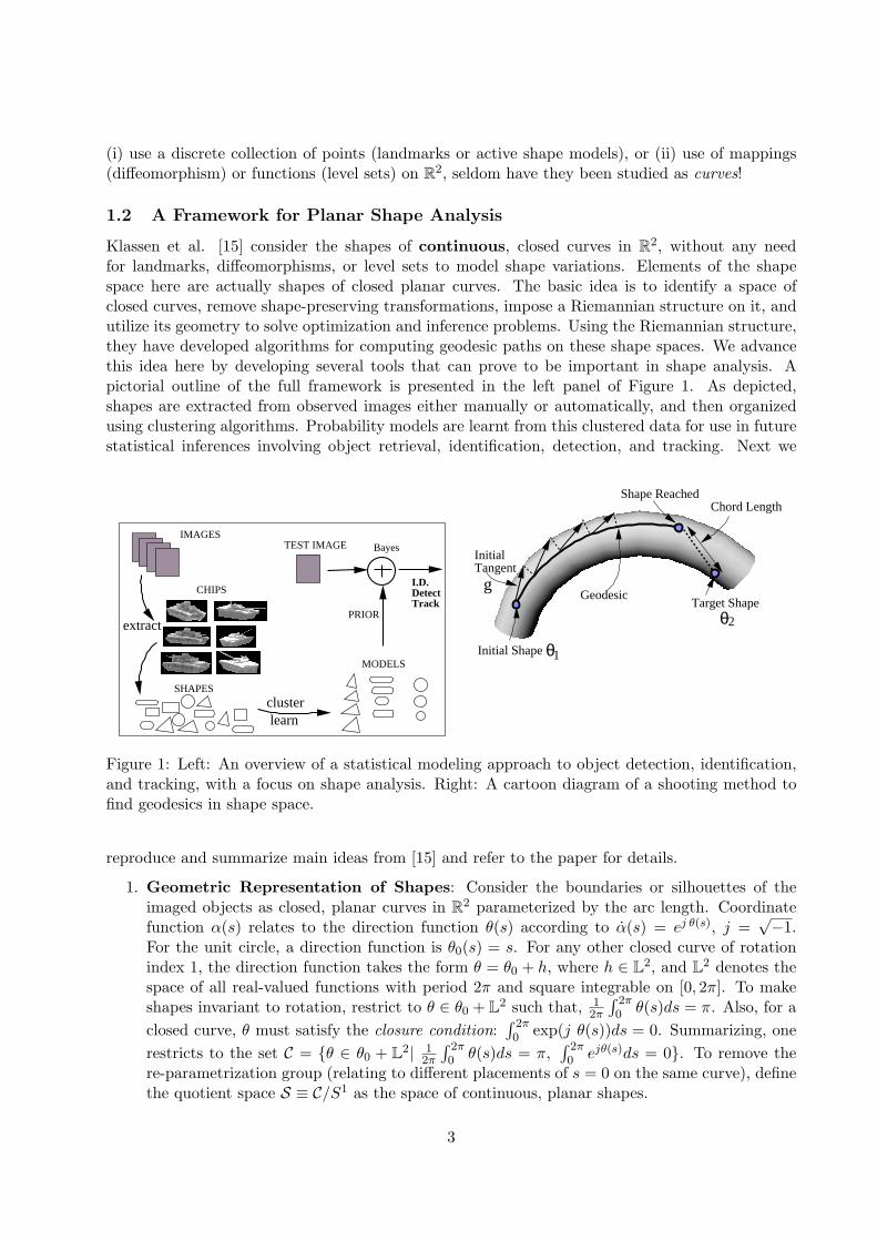
Klassen et al. [15] consider the shapes of continuous, closed curves in R2, without any needfor landmarks, diffeomorphisms, or level sets to model shape variations. Elements of the shapespace here are actually shapes of closed planar curves. The basic idea is to identify a space ofclosed curves, remove shape-preserving transformations, impose a Riemannian structure on it, andutilize its geometry to solve optimization and inference problems. Using the Riemannian structure,they have developed algorithms for computing geodesic paths on these shape spaces. We advancethis idea here by developing several tools that can prove to be important in shape analysis. Apictorial outline of the full framework is presented in the left panel of Figure 1. As depicted,shapes are extracted from observed images either manually or automatically, and then organizedusing clustering algorithms. Probability models are learnt from this clustered data for use in futurestatistical inferences involving object retrieval, identification, detection, and tracking. Next we

IMAGES

CHIPS

SHAPES

clusterlearn

extract

MODELS

TEST IMAGE

PRIOR

I.D.DetectTrack

Bayes

Initial Shape

Target ShapeGeodesic

InitialTangent

Chord LengthShape Reached

θ1

θ2

g

Figure 1: Left: An overview of a statistical modeling approach to object detection, identification,and tracking, with a focus on shape analysis. Right: A cartoon diagram of a shooting method tofind geodesics in shape space.

reproduce and summarize main ideas from [15] and refer to the paper for details.

1. Geometric Representation of Shapes: Consider the boundaries or silhouettes of theimaged objects as closed, planar curves in R2 parameterized by the arc length. Coordinatefunction α(s) relates to the direction function θ(s) according to α(s) = ej θ(s), j =

√−1.For the unit circle, a direction function is θ0(s) = s. For any other closed curve of rotationindex 1, the direction function takes the form θ = θ0 + h, where h ∈ L2, and L2 denotes thespace of all real-valued functions with period 2π and square integrable on [0, 2π]. To makeshapes invariant to rotation, restrict to θ ∈ θ0 + L2 such that, 1

2π

∫ 2π0 θ(s)ds = π. Also, for a

closed curve, θ must satisfy the closure condition:∫ 2π0 exp(j θ(s))ds = 0. Summarizing, one

restricts to the set C = {θ ∈ θ0 + L2| 12π

∫ 2π0 θ(s)ds = π,

∫ 2π0 ejθ(s)ds = 0}. To remove the

re-parametrization group (relating to different placements of s = 0 on the same curve), definethe quotient space S ≡ C/S1 as the space of continuous, planar shapes.

3

For an observed contour, denoted by a set of non-uniformly sampled points in R2, one cangenerate a representative element θ ∈ S as follows. For each neighboring pair of points,compute the chord angle θi and the Euclidean distance si between them. Then, fit a smoothθ function, e.g. using splines, to the graph formed by {(si, θi)} . Finally, resample θ uniformly(using arc-length parametrization) and project onto S.

2. Geodesic Paths Between Shapes: An important tool in a Riemannian analysis of shapesis to construct geodesic paths between arbitrary shapes. Klassen et al. [15] approximategeodesics on S by successively drawing infinitesimal line segments in L2 and projecting themonto S, as depicted in the right panel of Figure 1. For any two shapes θ1, θ2 ∈ S, they usea shooting method to construct the geodesic between them. The basic idea is search for atangent direction g at the first shape θ1, such that a geodesic in that direction reaches thesecond shape θ2, called target shape, in unit time. This search is performed by minimizing a“miss function”, defined as a L2 distance between the shape reached and θ2, using a gradientprocess. The geodesic is with respect to the L2 metric 〈g1, g2〉 =

∫ 2π0 g1(s)g2(s)ds on the

tangent space of S. This choice implies that a geodesic between two shapes is the path thatuses minimum energy to bend one shape into the other.

We will use the notation Ψ(θ, g, t) for a geodesic path starting from θ ∈ S, in the directiong ∈ Tθ(S), as a function of time t. Here Tθ(S) is the space of tangents to S at the pointθ. In practice, the function g is represented using an orthogonal expansion according tog(s) =

∑∞i=1 xiei(s), where {ei, i = 1, . . . , } forms an orthonormal basis of Tθ(S) and the

search for g is performed via a search for corresponding x = {x1, x2, . . . , }. An additionalsimplification is to let {ei} be a basis for L2, represent g using this basis, and subtractits projection onto the normal space at θ to obtain a tangent vector g. On a desktop PCwith Pentium IV 2.6GHz processor, it takes on average 0.065 seconds to compute a geodesicbetween any two shapes. In this experiment, the direction functions were sampled at 100points each and g is approximated using 100 Fourier terms.

Empirical evidence motivates us to consider shapes of two curves that are mirror reflectionsof each other as equivalent. For a θ ∈ S, its reflection is given by: θR(s) = 2π− θ(2π− s). Tofind a geodesic between two shapes θ1, θ2 ∈ S, we construct two geodesics: one between θ1

and θ2, and the other between θ1 and θ2R. The shorter of these two paths denotes a geodesicin the quotient space. With a slight abuse of notation, from here on, we will call the resultingquotient space as S.

3. Mean Shape in S: [15] suggests the use of Karcher mean to define mean shapes. Forθ1, . . . , θn in S, and d(θi, θj) the geodesic length between θi and θj , the Karcher mean is definedas the element µ ∈ S that minimizes the quantity

∑ni=1 d(θ, θi)2. A gradient-based, iterative

algorithm for computing the Karcher mean is presented in [16, 13] and is particularized toS in [15]. Statistical properties, such as bias and efficiency, of this estimator remain to beinvestigated.

1.3 Comparison with Previous Approaches

Some highlights of the above-mentioned approach are that it: (i) analyzes full curves and not acoarse collections of landmarks, i.e. there is no need to determine landmarks a-priori, (ii) com-pletely removes shape-preserving transformations from the representation and explicitly specifiesa shape space, (iii) utilizes nonlinear geometry of the shape space (of curves) to define and com-pute statistics, (iv) seeks full statistical frameworks and develops priors for future Bayesian infer-

4

ences, and (v) can be applied to real-time applications. Existing approaches seldom incorporateall of these features: Kendall’s representations are equipped with (ii)-(v) but using landmark-based representations; active shape models are fast and efficient but do not satisfy (ii) and (iii).Diffeomorphism-based models satisfy (i)-(iv) and can additionally take into account image inten-sities, but are currently slow for real-time applications. Curvature scale space methods are notequipped with either (iii) or (iv). It must be noted that for certain specific applications, existingapproaches may suffice or maybe more efficient than the proposed approach. For example, forretrieving shapes from a database, a simple metric using either Fourier descriptors or a PCA of co-ordinate vectors, or scale-space shape representations, may prove sufficient. However, the proposedapproach is intended as a comprehensive framework to handle a wide variety of applications.

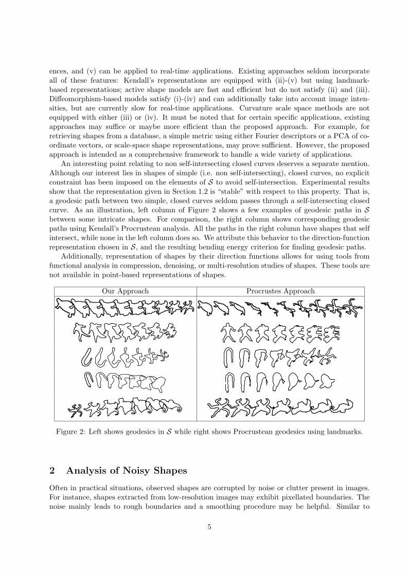
An interesting point relating to non self-intersecting closed curves deserves a separate mention.Although our interest lies in shapes of simple (i.e. non self-intersecting), closed curves, no explicitconstraint has been imposed on the elements of S to avoid self-intersection. Experimental resultsshow that the representation given in Section 1.2 is “stable” with respect to this property. That is,a geodesic path between two simple, closed curves seldom passes through a self-intersecting closedcurve. As an illustration, left column of Figure 2 shows a few examples of geodesic paths in Sbetween some intricate shapes. For comparison, the right column shows corresponding geodesicpaths using Kendall’s Procrustean analysis. All the paths in the right column have shapes that selfintersect, while none in the left column does so. We attribute this behavior to the direction-functionrepresentation chosen in S, and the resulting bending energy criterion for finding geodesic paths.

Additionally, representation of shapes by their direction functions allows for using tools fromfunctional analysis in compression, denoising, or multi-resolution studies of shapes. These tools arenot available in point-based representations of shapes.

Our Approach Procrustes Approach

Figure 2: Left shows geodesics in S while right shows Procrustean geodesics using landmarks.

2 Analysis of Noisy Shapes

Often in practical situations, observed shapes are corrupted by noise or clutter present in images.For instance, shapes extracted from low-resolution images may exhibit pixellated boundaries. Thenoise mainly leads to rough boundaries and a smoothing procedure may be helpful. Similar to

5

considerations in image denoising and restoration, a balance between smoothing and preservationof true edges is required, and the required amount of smoothing is difficult to predict in practice.In this section, we briefly discuss three ways to avoid certain noise effects:1. Robust Extraction: Use a smoothness prior on shapes during Bayesian extraction of shapes.For a shape denoted by θ, one can use elastic energy, define as

∫θ(s)2ds, as a roughness prior for

Bayesian extraction of shapes from images.2. Shape Denoising: Since shapes are represented as parameterized direction functions, one canuse tools from functional analysis for denoising. In case the extracted shapes have rough parts,one can replace them with their smooth approximations. A classical approach is to use waveletdenoising or Fourier smoothing. For example, shown in Figure 3 are examples of denoising thedirection function of a noisy shape using (i) wavelets (Daubechies, at level 4 in matlab), and (ii)Fourier expansion using first 20 harmonics.

0 50 100 150 200−2

−1.5

−1

−0.5

0

0.5

1

1.5

2

wavelet residualFourier residual

Figure 3: Noisy shape (left), wavelet denoised shape (second), Fourier denoised shape (third).Difference (residual) between noisy and denoised direction functions (right).

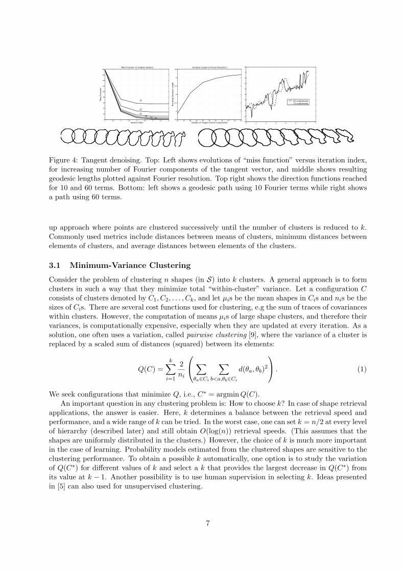
3. Tangent Denoising: Another possibility is to denoise the tangent function, rather than theoriginal direction functions (denoting shapes), as follows. A geodesic path between two givenshapes is found using a shooting method. By restricting the search for tangent direction g to aset of smooth functions, one can avoid certain noise effects. Shown in Figure 4 is an example ofthis idea, where the target shape is corrupted by noise. In top left panel, each curve shows thegradient-based evolution of “miss function” versus the iteration index. Different curves correspondto different number of terms used in Fourier expansion for the tangent direction; increasing thenumber of Fourier terms results in a better approximation of optimal g, and a smaller value of“miss” function. Top middle panel shows resulting geodesic lengths plotted against the Fourierresolution. A tangent function with smaller Fourier terms can help avoid the problem of over-fitting that often occurs with the noisy data. Bottom figures show the resulting geodesics for twodifferent tangent resolutions: the left path results from restricting the tangent direction to 10 terms,and the right path shows over fitting to noise in the target shape using 60 terms. Top right showsthe direction functions reached in unit time for these two cases.

3 Problem 1: Shape Clustering

An important need in statistical shape studies is to classify and cluster observed shapes. In thissection, we develop an algorithm for clustering objects according to shapes of their boundaries.Classical clustering algorithms on Euclidean spaces are well researched and generally fall into twomain categories: partitional and hierarchical [12]. Assuming that the desired number k of clustersis known, partitional algorithms typically seek to minimize a cost function Qk associated with agiven partition of the data set into k clusters. Hierarchical algorithms, in turn, take a bottom-

6

1 1.5 2 2.5 3 3.5 4 4.5 50

20

40

60

80

100

120

140

160

180"Miss Function" vs Gradient Iteration

Iteration Index

"Mis

s F

unct

ion"

10

20

3040

50 6010 15 20 25 30 35 40 45 50 55 60

10.5

11

11.5

12

12.5

13

13.5Geodesic Length vs Fourier Resolution

Number of Tangent Fourier Components

Res

ultin

g G

eode

sic

Leng

th

0 1 2 3 4 5 6 7−2

−1

0

1

2

3

4

5

6

7

8

60 components10 components

Figure 4: Tangent denoising. Top: Left shows evolutions of “miss function” versus iteration index,for increasing number of Fourier components of the tangent vector, and middle shows resultinggeodesic lengths plotted against Fourier resolution. Top right shows the direction functions reachedfor 10 and 60 terms. Bottom: left shows a geodesic path using 10 Fourier terms while right showsa path using 60 terms.

up approach where points are clustered successively until the number of clusters is reduced to k.Commonly used metrics include distances between means of clusters, minimum distances betweenelements of clusters, and average distances between elements of the clusters.

3.1 Minimum-Variance Clustering

Consider the problem of clustering n shapes (in S) into k clusters. A general approach is to formclusters in such a way that they minimize total “within-cluster” variance. Let a configuration Cconsists of clusters denoted by C1, C2, . . . , Ck, and let µis be the mean shapes in Cis and nis be thesizes of Cis. There are several cost functions used for clustering, e.g the sum of traces of covarianceswithin clusters. However, the computation of means µis of large shape clusters, and therefore theirvariances, is computationally expensive, especially when they are updated at every iteration. As asolution, one often uses a variation, called pairwise clustering [9], where the variance of a cluster isreplaced by a scaled sum of distances (squared) between its elements:

Q(C) =k∑

i=1

2ni

∑

θa∈Ci

∑

b<a,θb∈Ci

d(θa, θb)2

. (1)

We seek configurations that minimize Q, i.e., C∗ = argminQ(C).An important question in any clustering problem is: How to choose k? In case of shape retrieval

applications, the answer is easier. Here, k determines a balance between the retrieval speed andperformance, and a wide range of k can be tried. In the worst case, one can set k = n/2 at every levelof hierarchy (described later) and still obtain O(log(n)) retrieval speeds. (This assumes that theshapes are uniformly distributed in the clusters.) However, the choice of k is much more importantin the case of learning. Probability models estimated from the clustered shapes are sensitive to theclustering performance. To obtain a possible k automatically, one option is to study the variationof Q(C∗) for different values of k and select a k that provides the largest decrease in Q(C∗) fromits value at k − 1. Another possibility is to use human supervision in selecting k. Ideas presentedin [5] can also used for unsupervised clustering.

7

3.2 Clustering Algorithm

We will take a stochastic simulated annealing approach to solve for C∗. Several authors haveexplored the use of annealing in clustering problems, including soft clustering [22], and deterministicclustering [9]. An interesting idea presented in [9] is to solve an approximate problem, termedmean-field approximation, where Q is replaced by a function in which the roles of elements θisare decoupled. The advantage is the resulting efficiency although it comes at the cost of error inapproximation.

We will minimize the clustering cost using a Markov chain search process on the configurationspace. The basic idea is to start with a configuration of k clusters and to reduce Q by re-arrangingshapes amongst the clusters. The re-arrangement is performed in a stochastic fashion using twokinds of moves. These moves are performed with probability proportional to the negative expo-nential of the Q-value of the resulting configuration. The two types of moves are:

1. Move a shape: Here we select a shape randomly and re-assign it to another cluster. Let Q(i)j

be the clustering cost when a shape θj is re-assigned to the cluster Ci keeping all other clustersfixed. If θj is not a singleton, i.e. not the only element in its cluster, then the transfer of

θj to cluster Ci is performed with probability: PM (j, i;T ) =exp(−Q

(i)j /T )

∑ki=1 exp(−Q

(i)j /T )

i = 1, 2, . . . , k.

Here T plays a role similar to temperature in simulated annealing. If θj is a singleton, thenmoving it is not allowed in order to fix the number of clusters at k.

2. Swap two shapes: Here we select two shapes randomly from two different clusters andswap them. Let Q(1) and Q(2) be the Q-values of the original configuration (before swapping)and the new configuration (after swapping), respectively. Then, swapping is performed withprobability: PS(T ) = exp(−Q(2)/T )∑2

i=1 exp(−Q(i)/T ).

Additional types of moves can also be used to improve the search over the configuration spacealthough their computational cost becomes a factor too. In view of the computational simplicityof moving a shape and swapping two shapes, we have restricted our algorithm to these two moves.

In order to seek global optimization, we have adopted a simulated annealing approach. That is,we start with a high value of T and reduce it slowly as the algorithm searches for configurations withsmaller dispersions. Additionally, the moves are performed according to an acceptance-rejectionprocedure that is a variant of more conventional simulated annealing (see for example, AlgorithmA.20, pg. 200 [21] for a conventional procedure). Here, the candidates are proposed randomly andaccepted according to certain probabilities (PM and PS are defined above). Although simulatedannealing and the random nature of the search help in avoiding local minima, the convergence toa global minimum is difficult to establish. As described in [21], the output of this algorithm is aMarkov chain that is neither homogeneous nor convergent to a stationary chain. If the temperatureT is decreased slowly, then the chain is guaranteed to converge to a global minimum. However,it is difficult to make explicit the required rate of decrease in T and instead we rely on empiricalstudies to justify this algorithm. First, we state the algorithm and then describe some experimentalresults.

Algorithm 1 For n shapes and k clusters, initialize by randomly distributing n shapes among kclusters. Set a high initial temperature T .1. Compute pairwise geodesic distances between all n shapes. This requires n(n − 1)/2 geodesiccomputations.2. With equal probabilities pick one of the two moves:

8

• Move a shape: Pick a shape θj randomly. If it is not a singleton in its cluster, thencompute Q

(i)j for all i = 1, 2, . . . , k. Compute the probability PM (j, i; T ) for all i = 1, . . . , k

and re-assign θj to a cluster chosen according to the probability PM .

• Swap two shapes: Select two clusters randomly, and select a shape from each. Computethe probability PS(T ) and swap the two shapes according to that probability.

3. Update the temperature using T = T/β and return to Step 2. We have used β = 1.0001.

It is important to note that once the pairwise distances are computed, they are not computed againin the iterations. Secondly, unlike k-mean clustering, the mean shapes are never calculated in thisclustering. These factors make Algorithm 1 efficient and effective in clustering diverse shapes.

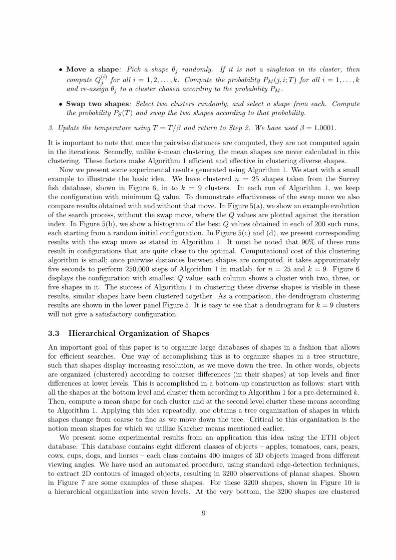
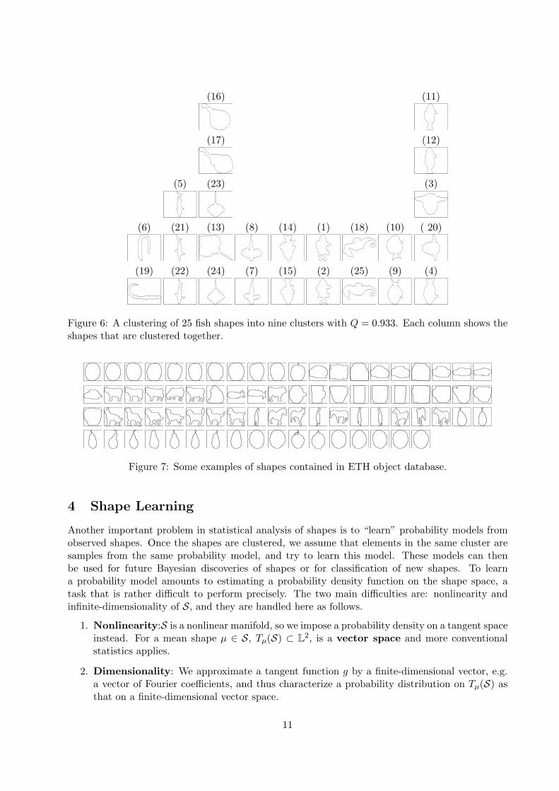
Now we present some experimental results generated using Algorithm 1. We start with a smallexample to illustrate the basic idea. We have clustered n = 25 shapes taken from the Surreyfish database, shown in Figure 6, in to k = 9 clusters. In each run of Algorithm 1, we keepthe configuration with minimum Q value. To demonstrate effectiveness of the swap move we alsocompare results obtained with and without that move. In Figure 5(a), we show an example evolutionof the search process, without the swap move, where the Q values are plotted against the iterationindex. In Figure 5(b), we show a histogram of the best Q values obtained in each of 200 such runs,each starting from a random initial configuration. In Figure 5(c) and (d), we present correspondingresults with the swap move as stated in Algorithm 1. It must be noted that 90% of these runsresult in configurations that are quite close to the optimal. Computational cost of this clusteringalgorithm is small; once pairwise distances between shapes are computed, it takes approximatelyfive seconds to perform 250,000 steps of Algorithm 1 in matlab, for n = 25 and k = 9. Figure 6displays the configuration with smallest Q value; each column shows a cluster with two, three, orfive shapes in it. The success of Algorithm 1 in clustering these diverse shapes is visible in theseresults, similar shapes have been clustered together. As a comparison, the dendrogram clusteringresults are shown in the lower panel Figure 5. It is easy to see that a dendrogram for k = 9 clusterswill not give a satisfactory configuration.

3.3 Hierarchical Organization of Shapes

An important goal of this paper is to organize large databases of shapes in a fashion that allowsfor efficient searches. One way of accomplishing this is to organize shapes in a tree structure,such that shapes display increasing resolution, as we move down the tree. In other words, objectsare organized (clustered) according to coarser differences (in their shapes) at top levels and finerdifferences at lower levels. This is accomplished in a bottom-up construction as follows: start withall the shapes at the bottom level and cluster them according to Algorithm 1 for a pre-determined k.Then, compute a mean shape for each cluster and at the second level cluster these means accordingto Algorithm 1. Applying this idea repeatedly, one obtains a tree organization of shapes in whichshapes change from coarse to fine as we move down the tree. Critical to this organization is thenotion mean shapes for which we utilize Karcher means mentioned earlier.

We present some experimental results from an application this idea using the ETH objectdatabase. This database contains eight different classes of objects – apples, tomatoes, cars, pears,cows, cups, dogs, and horses – each class contains 400 images of 3D objects imaged from differentviewing angles. We have used an automated procedure, using standard edge-detection techniques,to extract 2D contours of imaged objects, resulting in 3200 observations of planar shapes. Shownin Figure 7 are some examples of these shapes. For these 3200 shapes, shown in Figure 10 isa hierarchical organization into seven levels. At the very bottom, the 3200 shapes are clustered

9

0 0.5 1 1.5 2 2.5 3

x 104

0.8

1

1.2

1.4

1.6

1.8

2

2.2

2.4

2.6

No. of iterations

Qco

unt

Qmin

= 0.9476

0.92 0.94 0.96 0.98 1 1.02 1.04 1.060

5

10

15

20

25

30

35

40

45

50

Qmin

Cou

nt

No. of iterations = 200Q

min = 0.9476

Without Swapping

0 0.5 1 1.5 2 2.5 3

x 104

0.8

1

1.2

1.4

1.6

1.8

2

2.2

2.4

2.6

No. of iterations

Qco

unt

Qmin

= 0.9333

0.92 0.94 0.96 0.98 1 1.02 1.04 1.060

20

40

60

80

100

120

Qmin

Cou

nt

No. of iterations = 200

Qmin

= 0.9333

With Swapping

(a) (b) (c) (d)

3 20 4 11 12 13 23 24 16 17 7 5 21 22 1 2 14 15 9 10 8 6 19 18 25

0.2

0.3

0.4

0.5

0.6

0.7

0.8

Fish shapes

Dis

tanc

eDendrogram of 25 shapes

Figure 5: Top row: (a) A sample evolution of Q under Algorithm 1 without using the swap move.(b) A histogram of the minimum Q values obtained in 200 runs of Algorithm 1 (without swap move)each starting from a random initial condition. (c) and (d): sample evolution and a histogram of200 runs with the swap move. Lower row: A clustering result using the dendrogram function inmatlab.

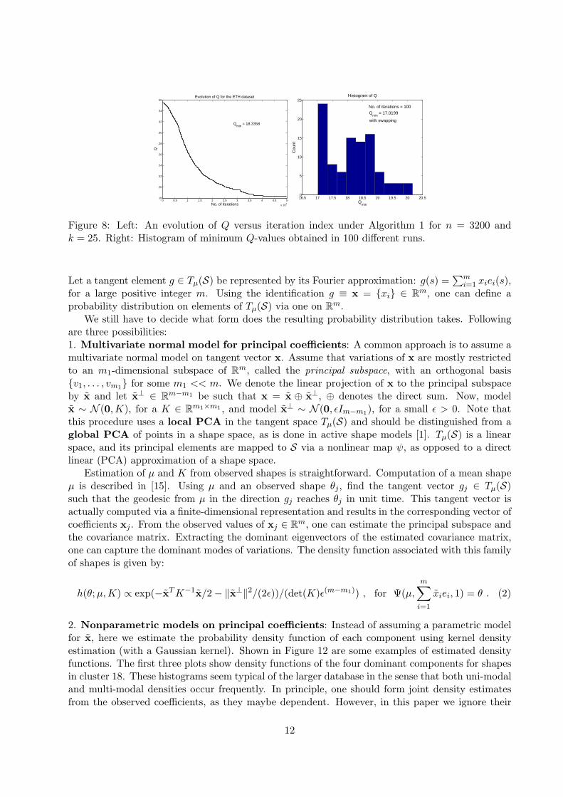
into k = 25 clusters. It currently takes approximately 100 hours on one computer to computeall pairwise geodesics for these 3200 shapes; one can use multiple desktop computers, or parallelcomputing, to accomplish this task more efficiently. Shown in Figure 8 left panel is an evolutionof Algorithm 1 for this data, and in Figure 9 are some examples shapes in some of these clusters.Figure 8 (right panel) shows a histogram of optimal Q-values obtained in 100 runs of Algorithm 1.The clustering in general agrees well with the known classification of these shapes. For example,apples and tomatoes are clustered together while cups and animals are clustered separately. It isinteresting to note that, with a few exceptions, shapes corresponding to different postures of animalsare also clustered separately. For example, shapes of cows sitting (cluster 25), animal shapes fromside views (cluster 6), and animal shapes from frontal views (cluster 23), are all clustered separately.It takes approximately 40 minutes in matlab to run 50K steps of Algorithm 1 with n = 3200 andk = 25. At the next level of hierarchy statistical means of elements in each cluster are computedand are clustered with n = 25 and k = 7. These 25 means are shown at level F in Figure 10. Thisprocess is repeated till we reach the top of the tree.

It is interesting to study the variations in shapes as we follow a path from top to bottom inthis tree. Three such paths from the tree are displayed in Figure 11, showing an increase in shapefeatures as we follow the path (drawn left to right here). This multi-resolution representation ofshapes has important implications. One is that very different shapes can be effectively comparedat a low resolution and high speed, while only similar shapes require high-resolution comparisons.

10

(16) (11)

(17) (12)

(5) (23) (3)

(6) (21) (13) (8) (14) (1) (18) (10) ( 20)

(19) (22) (24) (7) (15) (2) (25) (9) (4)

Figure 6: A clustering of 25 fish shapes into nine clusters with Q = 0.933. Each column shows theshapes that are clustered together.

Figure 7: Some examples of shapes contained in ETH object database.

4 Shape Learning

Another important problem in statistical analysis of shapes is to “learn” probability models fromobserved shapes. Once the shapes are clustered, we assume that elements in the same cluster aresamples from the same probability model, and try to learn this model. These models can thenbe used for future Bayesian discoveries of shapes or for classification of new shapes. To learna probability model amounts to estimating a probability density function on the shape space, atask that is rather difficult to perform precisely. The two main difficulties are: nonlinearity andinfinite-dimensionality of S, and they are handled here as follows.

1. Nonlinearity:S is a nonlinear manifold, so we impose a probability density on a tangent spaceinstead. For a mean shape µ ∈ S, Tµ(S) ⊂ L2, is a vector space and more conventionalstatistics applies.

2. Dimensionality: We approximate a tangent function g by a finite-dimensional vector, e.g.a vector of Fourier coefficients, and thus characterize a probability distribution on Tµ(S) asthat on a finite-dimensional vector space.

11

0 0.5 1 1.5 2 2.5 3 3.5 4 4.5 5

x 104

18

20

22

24

26

28

30

32

34

36

No. of iterations

Q

Evolution of Q for the ETH dataset

Qmin

= 18.3358

16.5 17 17.5 18 18.5 19 19.5 20 20.50

5

10

15

20

25

Qmin

Cou

nt

Histogram of Q

No. of iterations = 100

Qmin

= 17.0199

with swapping

Figure 8: Left: An evolution of Q versus iteration index under Algorithm 1 for n = 3200 andk = 25. Right: Histogram of minimum Q-values obtained in 100 different runs.

Let a tangent element g ∈ Tµ(S) be represented by its Fourier approximation: g(s) =∑m

i=1 xiei(s),for a large positive integer m. Using the identification g ≡ x = {xi} ∈ Rm, one can define aprobability distribution on elements of Tµ(S) via one on Rm.

We still have to decide what form does the resulting probability distribution takes. Followingare three possibilities:1. Multivariate normal model for principal coefficients: A common approach is to assume amultivariate normal model on tangent vector x. Assume that variations of x are mostly restrictedto an m1-dimensional subspace of Rm, called the principal subspace, with an orthogonal basis{v1, . . . , vm1} for some m1 << m. We denote the linear projection of x to the principal subspaceby x and let x⊥ ∈ Rm−m1 be such that x = x ⊕ x⊥, ⊕ denotes the direct sum. Now, modelx ∼ N (0,K), for a K ∈ Rm1×m1 , and model x⊥ ∼ N (0, εIm−m1), for a small ε > 0. Note thatthis procedure uses a local PCA in the tangent space Tµ(S) and should be distinguished from aglobal PCA of points in a shape space, as is done in active shape models [1]. Tµ(S) is a linearspace, and its principal elements are mapped to S via a nonlinear map ψ, as opposed to a directlinear (PCA) approximation of a shape space.

Estimation of µ and K from observed shapes is straightforward. Computation of a mean shapeµ is described in [15]. Using µ and an observed shape θj , find the tangent vector gj ∈ Tµ(S)such that the geodesic from µ in the direction gj reaches θj in unit time. This tangent vector isactually computed via a finite-dimensional representation and results in the corresponding vector ofcoefficients xj . From the observed values of xj ∈ Rm, one can estimate the principal subspace andthe covariance matrix. Extracting the dominant eigenvectors of the estimated covariance matrix,one can capture the dominant modes of variations. The density function associated with this familyof shapes is given by:

h(θ; µ,K) ∝ exp(−xT K−1x/2− ‖x⊥‖2/(2ε))/(det(K)ε(m−m1)) , for Ψ(µ,m∑

i=1

xiei, 1) = θ . (2)

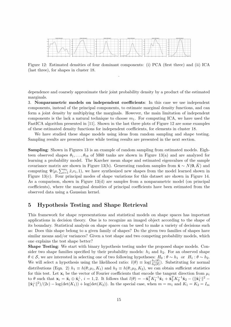
2. Nonparametric models on principal coefficients: Instead of assuming a parametric modelfor x, here we estimate the probability density function of each component using kernel densityestimation (with a Gaussian kernel). Shown in Figure 12 are some examples of estimated densityfunctions. The first three plots show density functions of the four dominant components for shapesin cluster 18. These histograms seem typical of the larger database in the sense that both uni-modaland multi-modal densities occur frequently. In principle, one should form joint density estimatesfrom the observed coefficients, as they maybe dependent. However, in this paper we ignore their

12

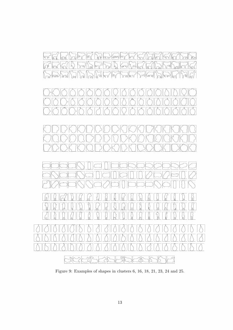
Figure 9: Examples of shapes in clusters 6, 16, 18, 21, 23, 24 and 25.

13

B

A

D

E

F

C

Figure 10: Hierarchical Clustering of 3200 shapes from the ETH-80 database

A B C D E F Database

Figure 11: Paths from top to bottom in the tree show increasing shape resolutions.

14

−2 −1 0 1 2 30.05

0.1

0.15

0.2

0.25

0.3

0.35

0.4Cluster=18,Comp=1

−2 −1 0 1 2 3 40

0.05

0.1

0.15

0.2

0.25

0.3

0.35

0.4Cluster=18,Comp=2

−3 −2 −1 0 1 2 30

0.1

0.2

0.3

0.4

0.5

0.6

0.7Cluster=18,Comp=3

−5 −4 −3 −2 −1 0 1 20

0.1

0.2

0.3

0.4

0.5

0.6

0.7Cluster=18,Comp=1

−2 −1 0 1 2 3 40

0.05

0.1

0.15

0.2

0.25

0.3

0.35

0.4Cluster=18,Comp=2

−2 −1 0 1 2 3 4 5 60

0.05

0.1

0.15

0.2

0.25

0.3

0.35

0.4

0.45Cluster=18,Comp=3

Figure 12: Estimated densities of four dominant components: (i) PCA (first three) and (ii) ICA(last three), for shapes in cluster 18.

.

dependence and coarsely approximate their joint probability density by a product of the estimatedmarginals.3. Nonparametric models on independent coefficients: In this case we use independentcomponents, instead of the principal components, to estimate marginal density functions, and canform a joint density by multiplying the marginals. However, the main limitation of independentcomponents is the lack a natural technique to choose m1. For computing ICA, we have used theFastICA algorithm presented in [11]. Shown in the last three plots of Figure 12 are some examplesof these estimated density functions for independent coefficients, for elements in cluster 18.

We have studied these shape models using ideas from random sampling and shape testing.Sampling results are presented here while testing results are presented in the next section.

Sampling: Shown in Figures 13 is an example of random sampling from estimated models. Eigh-teen observed shapes θ1, . . . , θ18 of M60 tanks are shown in Figure 13(a) and are analyzed forlearning a probability model. The Karcher mean shape and estimated eigenvalues of the samplecovariance matrix are shown in Figure 13(b). Generating random samples from x ∼ N(0, K) andcomputing Ψ(µ,

∑m1i=1 xivi, 1), we have synthesized new shapes from the model learned shown in

Figure 13(c). Four principal modes of shape variations for this dataset are shown in Figure 14.As a comparison, shown in Figure 13(d) are samples from a nonparametric model (on principalcoefficients), where the marginal densities of principal coefficients have been estimated from theobserved data using a Gaussian kernel.

5 Hypothesis Testing and Shape Retrieval

This framework for shape representations and statistical models on shape spaces has importantapplications in decision theory. One is to recognize an imaged object according to the shape ofits boundary. Statistical analysis on shape spaces can be used to make a variety of decisions suchas: Does this shape belong to a given family of shapes? Do the given two families of shapes havesimilar means and/or variances? Given a test shape and two competing probability models, whichone explains the test shape better?Shape Testing: We start with binary hypothesis testing under the proposed shape models. Con-sider two shape families specified by their probability models: h1 and h2. For an observed shapeθ ∈ S, we are interested in selecting one of two following hypotheses: H0 : θ ∼ h1 or H1 : θ ∼ h2.We will select a hypothesis using the likelihood ratio: l(θ) ≡ log(h1(θ)

h2(θ)). Substituting for normaldistributions (Eqn. 2) h1 ≡ h(θ;µ1,K1) and h2 ≡ h(θ; µ2, K2), we can obtain sufficient statisticsfor this test. Let xi be the vector of Fourier coefficients that encode the tangent direction from µi

to θ such that xi = xi ⊕ x⊥i , i = 1, 2. It follows that l(θ) = −xT1 K−1

1 x1 + xT2 K−1

2 x2 − (‖x⊥1 ‖2 −‖x⊥1 ‖2)/(2ε)− log(det(K1)) + log(det(K2)). In the special case, when m = m1 and K1 = K2 = Im

15

1 2 3 4 5 6 7 8 9 100

2

4

6

8

10

12

14

(a) (b)

(c) (d)

Figure 13: (a) 18 observed M60 tank shapes, (b) top shows the mean shape and bottom plots theprincipal eigenvalues of tangent covariance, (c) shows random samples from multivariate normalmodel, and (d) shows samples from a nonparametric model for principal coefficients.

Figure 14: Principal modes of variations in the 18 observed shapes shown in Figure 13.

(identity), the log-likelihood ratio is given by l(θ) = ‖x1‖2−‖x2‖2. Multiple hypothesis testing canbe accomplished similarly using the most likely hypothesis. The curved nature of the shape spaceS makes an analytical study of this test difficult. For instance, one may be interested in probabilityof type one error but that calculation requires a probability model on x2 when H0 is true.

We now present results from an experiment on hypothesis testing using the ETH database.In this experiment, we selected twelve out of 25 clusters shown at the bottom level of Figure 10.Shown in Figure 15 left side are mean shapes of these twelve clusters. In each class (or cluster), weused 50 shapes as training data for learning the shape models. A disjoint set of 2500 shapes (total),drawn randomly from these clusters, was used to test the classification performance; a correctclassification implies that the test shape was assigned to its own cluster. Shown in Figure 15 rightpanel is a plot of classification performance versus m1, the number of components used. This plotshows classification performances using: (i) multivariate normal model on tangent vectors, and(ii) nonparametric models on principal coefficients. We remark that, in this particular instance,nearest-mean classifier also performs well since that metric matches well with the cost function(Eqn. 1) used in clustering.Hierarchical Shape Retrieval: We want to use the idea of hypothesis testing in retrieving shapesfrom a database that has been organized hierarchically. In view of this structure, a natural way isto start at the top, compare the query with the shapes at each level, and proceed down the branchthat leads to the best match. At any level of the tree, there is a number, say k, of possible shapes,

16

3 4 5 6

9 15 16 18

21 22 23 24

0 5 10 15 20 25 30 350.1

0.2

0.3

0.4

0.5

0.6

0.7

0.8

0.9Hypothesis Testing Performance

Number of Components

Tes

t Per

form

ance

PCA NormalPCA Nonparam

Figure 15: Left: Mean shapes of 12 clusters. Right: Plots of classification performance versus thenumber of components used for: (i) multivariate normal modal on principal components, and (ii)independent non-parametric models on principal components.

and our goal is to find the shape that matches the query θ best. This can be performed usingk − 1 binary tests leading to the selection of the best hypothesis. In the current implementation,we have assumed a simplification that the covariance matrices for all hypotheses at all levels areidentity, and only the mean shapes are needed to organize the database. For identity covariances,the task of finding the best match at any level reduces to finding the nearest mean shape at thatlevel. Let µi be the given shapes at a level, and let xi be the Fourier vector that encode tangentdirection from θ to µi. Then, the nearest shape is indexed by i = argmini ‖xi‖. Proceed down thetree following the nearest shape µi at each level. This continues till we reach the last level and havefound the best overall match to the given query.

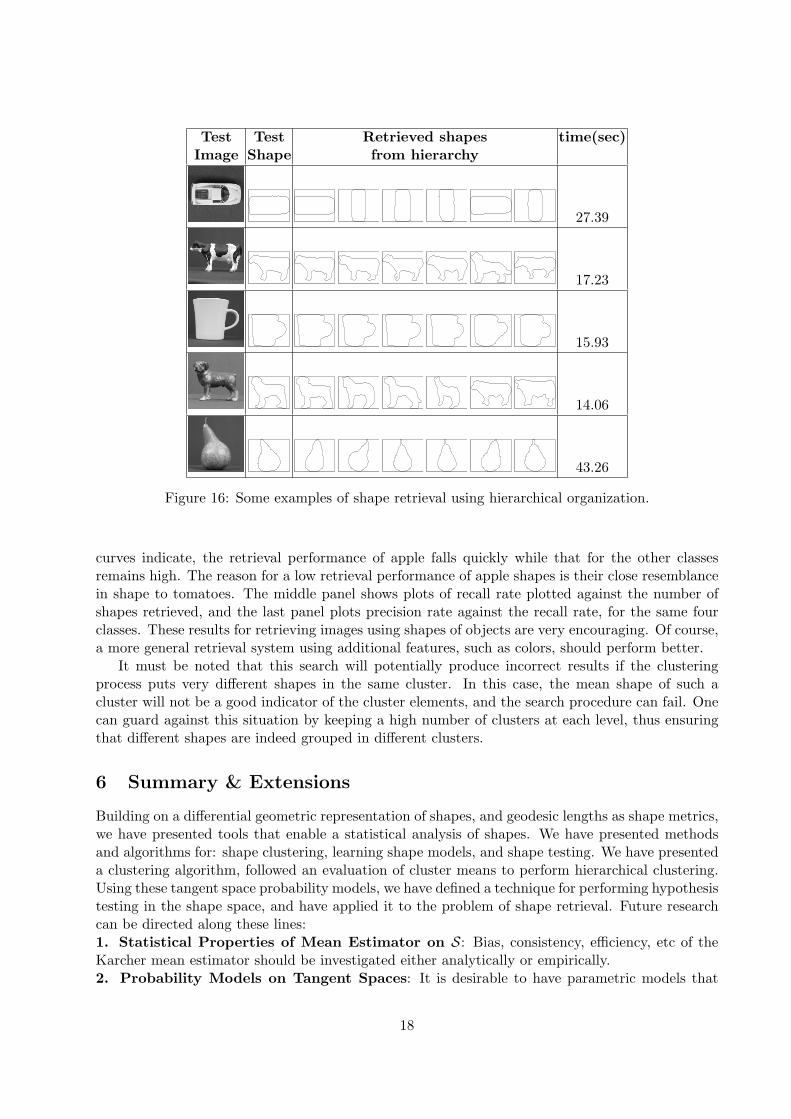
We have implemented this idea using test images from the ETH database. For each test image,we first extract the contour, compute its shape representation as θ ∈ S, and follow the tree, shownin Figure 10, for retrieving similar shapes from the database. Figure 16 presents some pictorialexamples from this experiment. Shown in the left panels are the original images and in the secondleft panels their automatically extracted contours. Third column shows six nearest shapes retrievedin response to the query. Finally, the last panel states the time taken for the hierarchical search.A summary of retrieval times is as follows:

Type of search time(sec) Type of search time(sec)exhaustive 126.64 worst case (hierarchical) 70.57

best case (hierarchical) 0.92 average (hierarchical) 24.84

The time for exhaustive search is computed by averaging the search time for all 3200 shapes, whilethe search times for hierarchical technique are for approximately 50 query images used in thisexperiment. These results show a significant improvement in the retrieval times while maintaininga good performance.

In this experiment, retrieval performance is defined with respect to the original labels, e.g.apple, cup, cow, pear, etc. Shown in Figure 17 are plots of retrieval performances, measured usingtwo different quantities. The first quantity is the precision rate, defined as the ratio of number ofrelevant shapes retrieved, i.e. shapes from the correct class, to the total number of shapes retrieved.Ideally, this quantity should be one, or quite close to one. The second quantity, called the recallrate, is the ratio of number of relevant shapes retrieved to the total number of shapes in that classin the database. Left panel in Figure 17 shows average variation of precision rate plotted againstthe number of shapes retrieved, for four different classes – apple, car, cup, and pear. As these

17

Test Test Retrieved shapes time(sec)Image Shape from hierarchy

27.39

17.23

15.93

14.06

43.26

Figure 16: Some examples of shape retrieval using hierarchical organization.

curves indicate, the retrieval performance of apple falls quickly while that for the other classesremains high. The reason for a low retrieval performance of apple shapes is their close resemblancein shape to tomatoes. The middle panel shows plots of recall rate plotted against the number ofshapes retrieved, and the last panel plots precision rate against the recall rate, for the same fourclasses. These results for retrieving images using shapes of objects are very encouraging. Of course,a more general retrieval system using additional features, such as colors, should perform better.

It must be noted that this search will potentially produce incorrect results if the clusteringprocess puts very different shapes in the same cluster. In this case, the mean shape of such acluster will not be a good indicator of the cluster elements, and the search procedure can fail. Onecan guard against this situation by keeping a high number of clusters at each level, thus ensuringthat different shapes are indeed grouped in different clusters.

6 Summary & Extensions

Building on a differential geometric representation of shapes, and geodesic lengths as shape metrics,we have presented tools that enable a statistical analysis of shapes. We have presented methodsand algorithms for: shape clustering, learning shape models, and shape testing. We have presenteda clustering algorithm, followed an evaluation of cluster means to perform hierarchical clustering.Using these tangent space probability models, we have defined a technique for performing hypothesistesting in the shape space, and have applied it to the problem of shape retrieval. Future researchcan be directed along these lines:1. Statistical Properties of Mean Estimator on S: Bias, consistency, efficiency, etc of theKarcher mean estimator should be investigated either analytically or empirically.2. Probability Models on Tangent Spaces: It is desirable to have parametric models that

18

0 50 100 150 200 250 300 350 400 4500.5

0.55

0.6

0.65

0.7

0.75

0.8

0.85

0.9

0.95

1

No. of Shapes retrieved

Pre

cisi

on r

ate

Precision rate against no. of shapes retrieved

AppleCarCupPear

0 50 100 150 200 250 300 350 400 4500

0.1

0.2

0.3

0.4

0.5

0.6

0.7

0.8

No. of Shapes retrieved

Rec

all r

ate

Recall rate against no. of shapes retrieved

AppleCarCupPear

0 0.1 0.2 0.3 0.4 0.5 0.6 0.7 0.80.5

0.55

0.6

0.65

0.7

0.75

0.8

0.85

0.9

0.95

1

Recall rate

Pre

cisi

on r

ate

Precision rate against the Recall rate

AppleCarCupPear

Figure 17: Left: precision rate versus number of shapes retrieved, middle panel: recall rate versusnumber retrieved, and right panel: precision rate versus recall rate.

capture the non-Gaussian behavior of observed tangents. Further investigations are needed todetermine if certain heavy-tailed models, such as Bessel K forms [8] or generalized Laplacian [17],or some other families, may better explain the observed data.3. Elastic Shapes: One limitation of the proposed approach is that arc-length parametrizationresults in shape comparisons solely on the basis of bending energies, without allowing for stretchingor compression. In some cases matching via stretching of shapes is more natural [2]. An extensionthat incorporates stretch elasticity by allowing reparameterizations of curves by arbitrary diffeomor-phisms is presented in [18]. A curve α ies represented by a pair (φ, θ) such that α(s) = eφ(s)ejθ(s).Appropriate constraints on (φ, θ) define a pre-shape manifold C, and the shape space is given byC/D, where D is the group of diffeomorphisms from [0, 1] to itself. The action of a diffeomorphismγ on a shape representation is given by: (φ, θ) = (φ ◦ γ + log(γ), θ ◦ γ). Computational details arepresented in [18].

Acknowledgement

This research was supported the grants NSF (FRG) DMS-0101429, NMA 201-01-2010, NSF (ACT)DMS-0345242, and ARO W911NF-04-01-0268. We would like to thank the three reviewers for theirhelpful comments. We are also grateful to the producers of ETH, Surrey, and AMCOM databases.

References

[1] T. F. Cootes, C. J. Taylor, D. H. Cooper, and J. Graham. Active shape models: Their trainingand application. Computer vision and image understanding, 61(1):38–59, 1995.

[2] R. H. Davies, C. J. Twining, P. D. Allen, T. F. Cootes, and C. J. Taylor. Building optimal2D statistical shape models. Image and Vision Computing, 21:1171–82, 2003.

[3] I. L. Dryden and K. V. Mardia. Statistical Shape Analysis. John Wiley & Son, 1998.

[4] N. Duta, A. K. Jain, and M.-P. Dubuisson-Jolly. Automatic construction of 2D shape models.IEEE Transactions on Pattern Analysis and Machine Intelligence, 23(5), 2001.

[5] M. A. T. Figueiredo and A. K. Jain. Unsupervised learning of finite mixture models. IEEETransactions on Pattern Analysis and Machine Intelligence, 24(3), 2002.

19

[6] U. Grenander. General Pattern Theory. Oxford University Press, 1993.

[7] U. Grenander and M. I. Miller. Computational anatomy: An emerging discipline. Quarterlyof Applied Mathematics, LVI(4):617–694, 1998.

[8] U. Grenander and A. Srivastava. Probability models for clutter in natural images. IEEETransactions on Pattern Analysis and Machine Intelligence, 23(4):424–429, April 2001.

[9] T. Hofmann and J. M. Buhmann. Pairwise data clustering by deterministic annealing. IEEETransactions on Pattern Analysis and Machine Intelligence, 19(1):1–14, 1997.

[10] A. Holboth, J. T. Kent, and I. L. Dryden. On the relation between edge and vertex modeliingin shape analysis. Scandinavian Journal of Statistics, 29:355–374, 2002.

[11] A. Hyvarinen. Fast and robust fixed-point algorithm for independent component analysis.IEEE Transactions on Neural Networks, 10:626–634, 1999.

[12] A. K. Jain and R. C. Dubes. Algorithms for Clustering Data. Prentice-Hall, 1988.

[13] H. Karcher. Riemann center of mass and mollifier smoothing. Communications on Pure andApplied Mathematics, 30:509–541, 1977.

[14] J. T. Kent and K. V. Mardia. Shape, Procrustes tangent projections and bilateral symmetry.Biometrika, 88:469–485, 2001.

[15] E. Klassen, A. Srivastava, W. Mio, and S. Joshi. Analysis of planar shapes using geodesicpaths on shape spaces. IEEE Pattern Analysis and Machiner Intelligence, 26(3):372–383,March, 2004.

[16] H. L. Le and D. G. Kendall. The Riemannian structure of Euclidean shape spaces: a novelenvironment for statistics. Annals of Statistics, 21(3):1225–1271, 1993.

[17] S G Mallat. A theory for multiresolution signal decomposition: The wavelet representation.IEEE Trans. on Pattern Analysis and Machine Intelligence, 11:674–693, 1989.

[18] W. Mio and A. Srivastava. Elastic string models for representation and analysis of planarshapes. In Proc. of IEEE Computer Vision and Pattern Recognition, 2004.

[19] W. Mio, A. Srivastava, and X. Liu. Learning and Bayesian shape extraction for object recog-nition. In Proc. of European conference on Computer Vision, pages Part IV, 62–73. SpringerVerlag, LNCS 3024, Eds: T. Pajdla and J. Matas, 2004.

[20] F. Mokhtarian. Silhouette-based isolated object recognition through curvature scale space.IEEE Trans. of Pattern Analysis and Machine Intelligence, 17(5):539–544, 1995.

[21] C. P. Robert and G. Casella. Monte Carlo Statistical Methods. Springer Text in Stat., 1999.

[22] K. Rose. Deterministic annealing for clustering, compression, classification, regression, andrelated optimization problems. Proceedings of IEEE, 86(11):2210–2239, 1998.

[23] C. G. Small. The Statistical Theory of Shape. Springer, 1996.

20