(2007) 272–286www.elsevier.com/locate/marchem

Marine Chemistry 106

Statistical process control in assessing production and dissolutionrates of biogenic silica in marine environments

Marc Elskens a,⁎, Anouk de Brauwere a, Charlotte Beucher b,1, Rudolph Corvaisier b,Nicolas Savoye a,2, Paul Tréguer b, Willy Baeyens a

a Laboratory for Analytical and Environmental Chemistry, Vrije Universiteit Brussel, Pleinlaan 2 B-1050 Brussels, Belgiumb CNRS UMR 6539, Laboratoire des Sciences de l'Environnement Marin, Université de Bretagne Occidentale,

Institut Universitaire Européen de la Mer, Technopôle Brest-Iroise, Place Copernic, 29280 Brest, France

Received 22 September 2005; received in revised form 30 October 2006Available online 26 January 2007

Abstract

This paper provides pieces of advice on the practices of quality assurance and quality control in assessing production anddissolution rates of biogenic silica in marine waters with stable isotope techniques. The objective is to make a rigorous contributionto the interpretation of 30Si isotopic measurements including modelling and uncertainty analyses. The results are illustrated withreal data taken from Beucher et al. [Beucher, C., Tréguer, P., Corvaisier, R., Hapette, A/-M., Elskens, M., 2004a. Production anddissolution of biogenic silica in a coastal ecosystem of western Europe. Marine Ecology Progress Series 267:57–69.]. Prior to theflux rate assessment, there are a number of analytical considerations required for screening between optimal and defectiveexperimental conditions. Three indexes were proposed to check the relevance of underlying assumptions when dealing with 30Sitracer enrichment and dilution techniques. Afterwards for extracting rate values from measurements, it is necessary to postulate amodel, and if required an optimization method. Various models and formulae were compared for their precision and accuracy. Itwas shown that oversimplified models risk bias when their underlying assumptions are violated, but overly complex models canmisinterpret part of the random noise as relevant processes. Therefore, none of the solutions can a priori be rejected, but eachshould statistically be assessed with hypothesis testing. A weighted least squares regression strategy combining an analysis of thestandardized residuals and cost function (sum of the weighted least squares residuals) was used to select optimal solution subsetscorresponding to a given data set, i.e. the solution that uses the most relevant processes and which was tested for the presence ofoutliers (observations or measurements with undue influence in the flux rate assessment).© 2007 Elsevier B.V. All rights reserved.

Keywords: Tracer method; Stable isotope; Biogenic silica; Modelling

⁎ Corresponding author.E-mail address: melskens@vub.ac.be (M. Elskens).

1 Now at: Marine Science Institute, University of California, SantaBarbara, California 93106, United States.2 Now at: OASU, UMR EPOC, Université Bordeaux 1, CNRS,

Station Marine d'Arcachon, 33120 Arcachon, France.

0304-4203/$ - see front matter © 2007 Elsevier B.V. All rights reserved.doi:10.1016/j.marchem.2007.01.008

1. Introduction

Since the pioneering work of Goering et al. (1973),stable isotopes 29Si and 30Si have been used to assesstransformation rates of biogenic silica (BSiO2) andsilicic acid (H4SiO4) in several marine ecosystems(Nelson and Gordon, 1982; Nelson et al., 1991). Laterthe development of radioactive 32Si isotope measuring

273M. Elskens et al. / Marine Chemistry 106 (2007) 272–286

procedures (Tréguer et al., 1991; Brzezinski andPhillips, 1997) has significantly improved the measure-ments of biogenic silica production rates (e.g. Brze-zinski et al., 1998; Quéguiner, 2001). However, there areseveral reasons to further use stable isotopes in routinemeasurements; (1) their use remains the only way tomeasure silica dissolution rates, and (2) they are nothazardous. This does not exclude that some inherentdifficulties remain, for example, measuring rates of nearsurface silica dissolution with isotope dilution and massspectrometry remains a difficult task because this ratemay be low, especially in offshore waters. It isanticipated that increased experimental ingenuity willovercome some of these technical difficulties. In thatway, refined analytical methods were recently devel-oped based on thermal ionisation-mass spectrometry,TI-MS (Corvaisier et al., 2005) and high resolution-inductively coupled plasma-mass spectrometry, HR-ICP-MS (Klemens and Heumann, 2001; Cardinal pers.comm.).

In order to extract values for the flux rates(production and dissolution of biogenic silica) fromthose measurements, it is necessary to postulate a model.In addition, an appropriate optimization method shouldbe chosen with care since the numerical values for theparameter estimates largely depend upon the criteria andmethods used to match model and measurements(Janssen and Heuberger, 1995). Because pathways thatcontrol nutrient cycling in aquatic systems are seldomunivocal, there is understandably some disagreementabout the best approach to model these processes(number of parameters, number of equations…). Thefirst goal of this paper is to compare the estimationbehaviour of the basic model approach for assessingsilicic acid uptake by phytoplankton (Nelson andGoering, 1977a) and silica dissolution (Nelson andGoering, 1977b) with a nonlinear two compartmentalmodel previously described in Beucher et al. (2004a,b)and de Brauwere et al. (2005a). Since the notion of a“true model” is typically a fiction for real-life applica-tion, usefulness rather than trueness should be theguiding principle in developing and comparing models.Clearly, there is a need for criteria allowing an objectiveassessment of the model results (Elskens et al., 2005)and a well-defined model selection strategy (deBrauwere et al., 2005b). Therefore, the second goal ofthis paper is to present a series of data processingtechniques that are relevant from a user's and manage-ment's perspective. Namely, which strategy should beapplied to select an appropriate model solution? Howcan systematic errors or model failure be detected withreal data? What confidence can be placed into the final

model outcome? Which data can be considered asoutliers and should be removed?

The result of this quality assessment is illustratedwith real data reported in Beucher et al. (2004a) anddiscussed in relation to quality assurance for researchand development and non-routine analysis.

2. Material and methods

2.1. Experimental design and assumptions

The enrichment and isotope dilution technique,which is applied for the simultaneous determination ofbiosilica production and dissolution rates, involves theaddition of enriched Na2

30SiO3 solutions to a watersample, and after some period of incubation measuring(i) the 30Si incorporated into the particulate material(=uptake) and (ii) the coincident tracer dilution in thedissolved pool due to dissolution of unlabelled biosilica.The changes in concentration and isotopic abundance ofH4SiO4 acid and BSiO2 are assessed by measuring themjust after the spike (t=0) and after a given incubationperiod, usually 24 h. Isotopic abundance is defined as100% [30Si]/([28Si] + [29Si] + [30Si]). The analyticalprocedures are described in Corvaisier et al. (2005).Before these measurements can be interpreted, a numberof basic statements about the behaviour of the isotopictracer must be postulated: (i) the tracer undergoes thesame transformations (transfer reactions) as the unla-belled substrate, i.e. isotope effects are negligible, (ii)there is no exchange of the isotope between the labelledsubstance and other substances in the system, (iii) thetracer is initially not in equilibrium with the systemunder study, and its change over time is quantifiable,(iv) regeneration has the background ratio of abundance,i.e. it consists of non-enriched compounds, and (v)the tracer addition does not perturb the steady stateexisting in the system as a whole, i.e., there are nosignificant perturbations to compartments and theirtransformations.

These are basic assumptions in experimental designsinvolving isotope enrichment and dilution procedures(e.g. Harrison, 1983). For silicon isotopes, assumptions(i–ii) are not seriously violated (De La Rocha et al.,1997). Although assumptions (i) and (iv) may appearcontradictory, it is not. The rationale of assumption (iv)is the following. In order to solve the model equations,the abundance at which dissolution of BSiO2 proceedsmust be fixed. By the uptake of H4SiO4, diatoms buildup their frustules composed of amorphous silica. Whilediatoms are alive, an organic coating protects silicafrom dissolution (Bidle and Azam, 1999). It is usually

274 M. Elskens et al. / Marine Chemistry 106 (2007) 272–286

assumed that only dead diatoms can dissolve. Moreover,Beucher et al. (2004b) showed that the dissolution ratecorrelated to the percentage of dead diatom. It is,therefore, reasonable that a finite period of time isrequired before any of the 30Si-enriched atoms willappear in the regenerated H4SiO4. The validity ofassumption (iii) may be a problem when long incubationperiod is used and abundance of the tracer, as well asconcentration of the labelled substrate change substan-tially. Violation of assumption (iv) also becomessignificant under these circumstances. For assumption(v), “true” tracer additions, considered usually as <10%of the ambient concentration (Dugdale and Goering,1967), is not always achievable. As a consequence,changes in substrate concentration and flux rates may besignificant. To what extend violations of those assump-tions will create significant biases in flux rate calcula-tions will undoubtedly vary between systems, butseveral criteria are useful for screening between optimaland defective experimental conditions (see Section 2.3).

2.2. Model description

For the sake of clarity all symbols used hereafter aredefined in the glossary and their notations appliedthroughout.

2.2.1. The Nelson and Goering formulaeThe classical approach for assessing silicic acid uptake

by phytoplankton (Nelson and Goering, 1977a) and silicadissolution (Nelson and Goering, 1977b) is derived fromthe following one compartmental model:

Yðϕ;&ϕÞ½C &C� ð1Þ

The differential equations associated with this modelare:

A&C

At¼ −

ð&CðtÞ−&/Þd/CðtÞ

ACAt

¼ /

8><>: ð2Þ

Straightforward integration of Eq. (2) yields thefollowing mass and isotopic balances:

&CðtÞd CðtÞ ¼ &Cð0Þd Cð0Þ þ &/d /d tCðtÞ ¼ Cð0Þ þ /d t

�ð3Þ

Eq. (3) can be rewritten with appropriate symbols foran enrichment experiment in the particulate phaseaccording to:

C ¼ BSiO2; &Cð0Þ ¼ 0; &CðtÞ ¼ &BSiO2ðtÞ;&/ ¼ &H4SiO4ð0Þ; / ¼ u ð4Þ

or for an isotope dilution experiment in the dissolvedphase according to:

C ¼ H4SiO4; &Cð0Þ ¼ &H4SiO4ð0Þ;&CðtÞ ¼ &H4SiO4ðtÞ; &/ ¼ 0; / ¼ d ð5ÞFrom Eqs. (3)–(5), uptake of H4SiO4 and dissolution

rates of BSiO2 can be solved for as follows:

u ¼BSiO2ðtÞd &BSiO2ðtÞ

td &H4SiO4ð0ÞBSiO2ð0Þd &BSiO2ðtÞ

td ð&H4SiO4ð0Þ−&BSiO2ðtÞÞ

8>><>>:

d ¼H4SiO4ðtÞd ð&H4SiO4ð0Þ−&H4SiO4ðtÞÞ

td &H4SiO4ð0ÞH4SiO4ð0Þd ð&H4SiO4ð0Þ−&H4SiO4ðtÞÞ

td &H4SiO4ðtÞ

8>><>>:

ð6Þ

Similar formulae have widely been applied to computenitrogen (Dugdale and Goering, 1967; Dugdale andWilkerson, 1986; Collos, 1987) and carbon (Collos andSlawyk, 1985; Legendre and Gosselin, 1996) transportrates in aquatic systems. It is noted, however, that two dif-ferent analytical solutions were gathered whether con-sidering the sample concentration at the beginning or theend of the incubation. Conceptually, these solutions shouldbe mathematically equivalent if the model correctly de-scribed the main features of production and dissolutionprocesses. In many cases, however, it is an approximation,and differences between formulae (6) may be ascribed toconcentration changes over the incubation period and iso-tope dilution effects. To correct for concentration changes,Nelson and Goering (1977a,b) recommend the use of thegeometric mean in computing rates:

u ¼ ðBSiO2ðOÞd BSiO2ðtÞÞ0:5d &BSiO2ðtÞtd &H4SiO4ð0Þ

d ¼ ðH4SiO4ð0Þd H4SiO4ðtÞÞ0:5d ð&H4SiO4ð0Þ−&H4SiO4ðtÞÞtd &H4SiO4ð0Þ

8>>><>>>:

ð7Þ

Alternatively, it is possible to handle both isotope dilu-tion and concentration changes with compartmental anal-ysis (Beucher et al., 2004a,b; de Brauwere et al., 2005a).

2.2.2. Two compartmental model for BSiO2 productionand dissolution

½H4SiO4 &H4SiO4 � Wðu;&H4SiO4 Þðd;&BSiO2 Þ

½BSiO2 &BSiO2 � ð8Þ

Important features of model (8) are that all Si atomsthat leave the dissolved phase are assumed to appear as

275M. Elskens et al. / Marine Chemistry 106 (2007) 272–286

particulate silica, and that dissolution is regarded asa process that transfers Si atoms from the particulate tothe dissolved pool. Analogous models or even morecomplicated ones were build-up to address the problemof N cycling in aquatic systems (Elskens et al., 2005).The differential equations associated with the twocompartment model are:

AH4SiO4

At¼ d−u

A&H4SiO4

At¼ −dd

&H4SiO4ðtÞH4SiO4ðtÞ

ABSiO2

At¼ u−d

A&BSiO2

At¼ dd

&BSiO2ðtÞBSiO2ðtÞ þ ud

&H4SiO4ðtÞ−&BSiO2ðtÞBSiO2ðtÞ

8>>>>>>>>><>>>>>>>>>:

ð9ÞWhen Eq. (9) is integrated, the relevant model

equations are:

H4SiO4ðtÞ ¼ H4SiO4ð0Þ þ ðd−uÞdt

&H4SiO4 ðtÞ ¼ &H4SiO4 0ð Þd 1þ d−uH4SiO4ð0Þ d t

� � du−d

BSiO2ðtÞ ¼ BSiO2ð0Þ þ ðu−dÞd t

&BSiO2 ðtÞ ¼&H4SiO4 ð0Þd H4SiO4ð0ÞBSiO2ð0Þ þ ðu−dÞd t d 1− 1þ d−u

H4SiO4ð0Þ d t� � u

u−d !

8>>>>>>>><>>>>>>>>:

ð10ÞThere are several methods to extract rates from this

system, since it involves four equations for merely twounknowns (u and d). Due to random and systematic vari-ations, there are differences between model results andmeasurements. Therefore, the best method is to seek thoseparameter-values that minimize all four equations simul-taneously, instead of solving 1 or 2 equations analytically.However, due to the second and the fourth equations in Eq.(10), themodel is nonlinear in the unknowns. To be solvedan iterative optimization algorithm must then be used.

It is noted that with the current experimental designonly the averaged rate over the incubation period can bedetermined, i.e. /ðu; dÞ ¼ 1

t

R t0 /ðtÞd dt. This is true

independently of the chosen model structure. To assessinstantaneous rates ϕ(t), a mechanism (e.g. first, secondorder, or saturation kinetic) for the transformationreactions must be postulated, but this requires time-series measurements.

2.3. Rules for the screening of experimental conditions

In Section 2.1, we have summarized 5 characteristicsof the behaviour of an “ideal” tracer to perform isotopeenrichment and dilution experiments. Violations of

these assumptions may generate significant biases inthe rate calculations. If isotope equilibrium is reached orapproached during an experiment, one cannot warrantthe flux rate-values (violation of assumption iii). For thesystem under study, isotope equilibrium is achievedafter 30Si enrichment, when the abundance of theparticulate phase (BSiO2) and dissolved phase (H4SiO4)becomes equal; the tracer is then said to be in a steadystate. A useful measure of this is given by the abundanceratio AR, a rescaled index varying between 0 and 1:

AR ¼ &H4SiO4ðtÞ−&BSiO2ðtÞ&H4SiO4ð0Þ

ð11Þ

When AR is close to 1, the tracer is far from equili-brium (optimal conditions). When AR moves towardszero, the tracer approaches steady state conditions. Thereare only informal guidelines for thresholds under whichvalues of AR should require attention.We suggest to high-light the data when AR<0.25. Likewise, a simple index(HL) based on the half-life and incubation period (Δt) canbe used to gauge the validity limit of assumption (iv).

HL ¼ BSiO2ð0Þ2dddDt

ð12Þ

with BSiO2 the biogenic Si concentration and d thedissolution rate.

If HL becomes ≤1 (i.e. more than half of the BSiO2

pool is recycled during the incubation time), violation ofassumption (iv) becomes likely, and the data should behighlighted. Violations of (iii and iv) are ofteninterrelated, and it is not unusual for a dataset to behighlighted by both criteria. Under these conditions, thelikelihood of gross errors is so serious that there is no realalternative than to reject the result of the experiment.Finally when the tracer addition (TA) is> than 10% of theambient H4SiO4 concentration (violation of assumptionv), flux rates should be considered as potential ones.

2.4. Assessment of model accuracy

In order to assess the discrepancy between theobservations yi and the model counterparts fmodel(xi,θ),we need some way to transform the residual (yi− fmodel

(xi,θ)) to a common scale on which we know what largeand small values are. An obvious approach is to define astandardized residual:

SRi ¼ yi−fmodelðxi; hÞri

ð13Þ

where σi should express the total standard deviation ofthe residual. This is achieved here by linearization of the

276 M. Elskens et al. / Marine Chemistry 106 (2007) 272–286

input noise on xi and adding them to the original outputnoise on yi (de Brauwere et al., 2005a):

r2i ¼ r2y;i þXni¼1

jAfmodelðxi; hÞAxi

j2d r2x;i ð14Þ

Substituting the u- and d-estimates from models (1)and (8) in their corresponding mass balance Eqs. (3) and(10) yields standardized residuals for concentration andabundance in the dissolved and particulate phases. Wechoose the standardized residuals for two reasons.Firstly, SRi solves the problem of scaling, i.e. if yi andσi2 are good estimates of the population's mean and

variance, then the SRi's can be interpreted as standardnormal deviates. The accuracy of the models towardsmeasurements was further assessed by inspecting theSRi distribution for a series of 53 experiments carriedout by Beucher et al. (2004a). If the models correctlydescribe the main features of uptake and dissolutionprocesses, it is expected that RSi-scores will besymmetrically distributed with a mean of zero. More-over, the meaning of the scores can be immediatelyappreciated, e.g., absolute values of RSi≤1 would bevery common (≈68% of the data) whereas absolutevalues of RSi>3 would be very rare (<0.27% of thedata) suggesting either model failure or outlyingmeasurements. This enables a direct comparisonbetween models that are solved algebraically andnumerically. Secondly SRi has a natural interpretationin the context of the residual cost function CF, which isused to estimate the model parameters in model (8):

CF ¼Xni¼1

SR2ic

Xni¼1

ðNð0; 1ÞÞ2 ¼ v2n−p ð15Þ

Depending on the assumption of the normal distribu-tion, which outliers apart seems to be justified inpractice, the CF has a chi-squared χ2 distribution withn−p degrees of freedom (Box, 1970; Rod and Hancil,1980), where n stands for the number of measurementsand p for the number of parameters in the model. Withthis information, it is possible to assess the “probability”of a residual cost function value. If the residual valuefalls beyond a chosen confidence limit, the results shouldbe rejected for being “unlikely” (de Brauwere et al.,2005b). For instance, if the residual value is significantlyhigher than expected, the remaining difference betweenmodel andmeasurements is too high to be explained onlyby stochastic measurement noise. This significantdifference between the expected and observed residualcost function is an indicator of systematic errors, and is

thus complementary to the SRi approach. Moreover, aswill be discussed later, the cost function approach is alsouseful for selecting relevant parameters within a givenmodel.

2.5. Assessment of model precision

Knowledge of model precision is necessary for theeffective judgment of the model results (e.g. compar-ison with specification limits) and for inter-comparisonof different model outcomes. From the outset, all thefactors that may contribute to uncertainty in the modelcalculations are expressed as standard deviations.While it cannot always be taken for granted thatthere exits a regular functional relationship betweenprecision and the concentration level of an analyte, theHorwitz function has shown that the relative standarddeviation (RSD) is useful in evaluating precision overa wide range of concentration (Horwitz, 1983;Thompson and Lowthian, 1997). For H4SiO4 determi-nations, Strickland and Parsons (1968) reported RSDvalues close to 2.5%. For BSiO2 determinations,Ragueneau and Tréguer (1994) reported RSD valuesclose to 10%. For isotopic analysis, results obtainedon Na2SiO3 standard solution indicated RSD less than0.5% (Corvaisier et al., 2005). However, actualprecision may be lower than the quoted value,particularly with 30Si enriched sample that has beenprocessed through all steps of the incubation protocol.An overall RSD of 2% appears, therefore, reasonablein estimating the Si isotopic composition of bothBSiO2 and H4SiO4. Model precision (propagation ofrandom error in calculations) is assessed with Monte-Carlo simulations. A number of random deviates (500)on concentrations and isotopic ratios were generatedby computer assuming normal distributions withknown mean and RSD. For each random deviation,the Si flux rates were calculated resulting in adistribution of best fit parameter values from whichthe statistical properties can be analyzed, and thus aquantification of the model precision can be achieved.

3. Results and discussion

3.1. Screening of experimental conditions

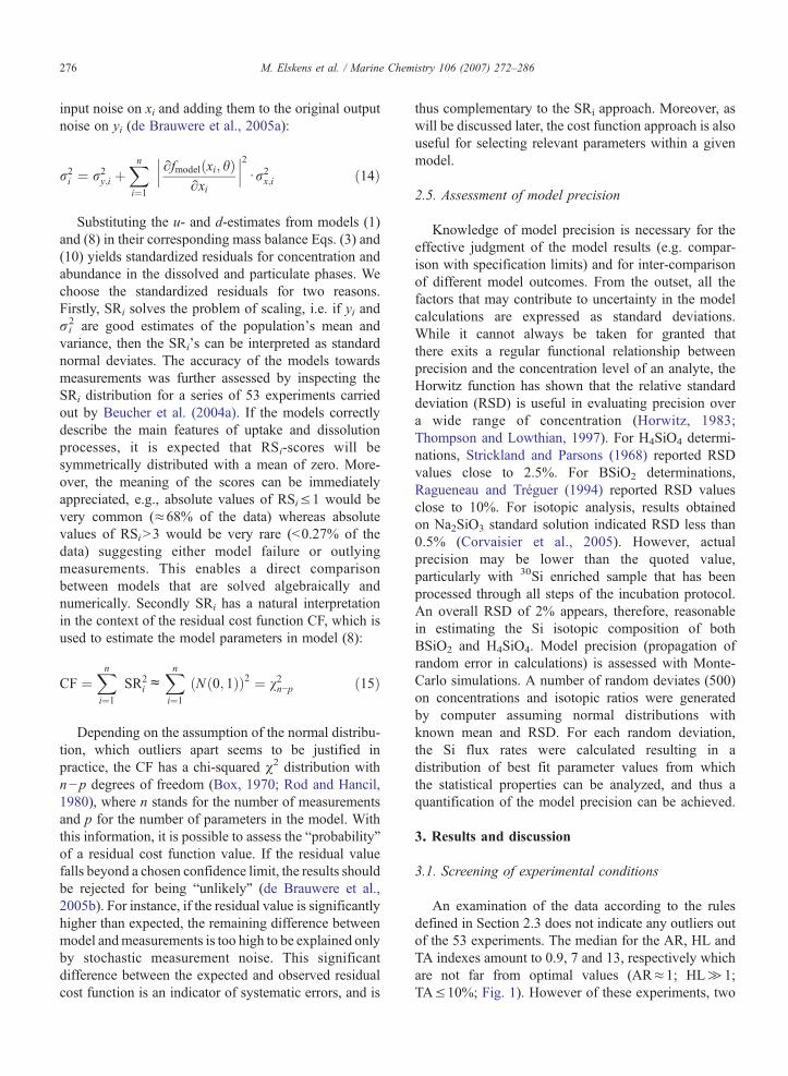
An examination of the data according to the rulesdefined in Section 2.3 does not indicate any outliers outof the 53 experiments. The median for the AR, HL andTA indexes amount to 0.9, 7 and 13, respectively whichare not far from optimal values (AR≈1; HL≫1;TA≤10%; Fig. 1). However of these experiments, two

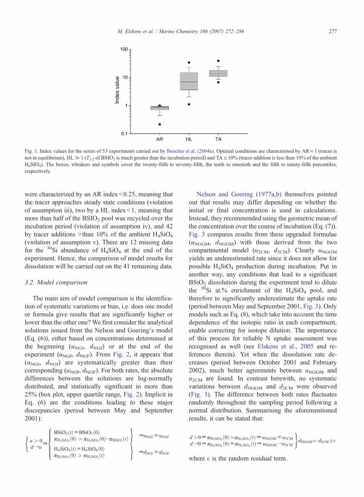
Fig. 1. Index values for the series of 53 experiments carried out by Beucher et al. (2004a). Optimal conditions are characterised by AR≈1 (tracer isnot in equilibrium), HL≫1 (T1/2 of BSIO2 is much greater than the incubation period) and TA≤10% (tracer addition is less than 10% of the ambientH4SIO4). The boxes, whiskers and symbols cover the twenty-fifth to seventy-fifth, the tenth to ninetieth and the fifth to ninety-fifth percentiles,respectively.

277M. Elskens et al. / Marine Chemistry 106 (2007) 272–286

were characterized by an AR index<0.25, meaning thatthe tracer approaches steady state conditions (violationof assumption iii), two by a HL index<1, meaning thatmore than half of the BSIO2 pool was recycled over theincubation period (violation of assumption iv), and 42by tracer additions >than 10% of the ambient H4SiO4

(violation of assumption v). There are 12 missing datafor the 30Si abundance of H4SiO4 at the end of theexperiment. Hence, the comparison of model results fordissolution will be carried out on the 41 remaining data.

3.2. Model comparison

The main aim of model comparison is the identifica-tion of systematic variations or bias, i.e. does one modelor formula give results that are significantly higher orlower than the other one? We first consider the analyticalsolutions issued from the Nelson and Goering's model(Eq. (6)), either based on concentrations determined atthe beginning (uNGI, dNGI) or at the end of theexperiment (uNGF, dNGF). From Fig. 2, it appears that(uNGI, dNGI) are systematically greater than theircorresponding (uNGF, dNGF). For both rates, the absolutedifferences between the solutions are log-normallydistributed, and statistically significant in more than25% (box plot, upper quartile range, Fig. 2). Implicit inEq. (6) are the conditions leading to these majordiscrepancies (period between May and September2001):

(u > 0dYu

Z

BSiO2ðtÞcBSiO2ð0Þ&H4SiO4 ð0Þ > &H4SiO4 ð0Þ−&BSiO2 ðtÞ

)ZuNGIHuNGF

H4SiO4ðtÞcH4SiO4ð0Þ&H4SiO4 ð0Þ > &H4SiO4 ðtÞ

)ZdNGIHdNGF

8>>>><>>>>:

Nelson and Goering (1977a,b) themselves pointedout that results may differ depending on whether theinitial or final concentration is used in calculations.Instead, they recommended using the geometric mean ofthe concentration over the course of incubation (Eq. (7)).Fig. 3 compares results from these upgraded formulae(uNGGM, dNGGM) with those derived from the twocompartmental model (u2CM, d2CM). Clearly uNGGMyields an underestimated rate since it does not allow forpossible H4SiO4 production during incubation. Put inanother way, any conditions that lead to a significantBSiO2 dissolution during the experiment tend to dilutethe 30Si at.% enrichment of the H4SiO4 pool, andtherefore to significantly underestimate the uptake rate(period betweenMay and September 2001, Fig. 3). Onlymodels such as Eq. (8), which take into account the timedependence of the isotopic ratio in each compartment,enable correcting for isotope dilution. The importanceof this process for reliable N uptake assessment wasrecognised as well (see Elskens et al., 2005 and re-ferences therein). Yet when the dissolution rate de-creases (period between October 2001 and February2002), much better agreements between uNGGM andu2CM are found. In contrast herewith, no systematicvariations between dNGGM and d2CM were observed(Fig. 3). The difference between both rates fluctuatesrandomly throughout the sampling period following anormal distribution. Summarising the aforementionedresults, it can be stated that:

d>0Z &H4SiO4 ð0Þ>&H4SiO4 ðtÞZ uNGGMbu2CMdY0Z &H4SiO4 ð0Þc&H4SiO4 ðtÞZ uNGGMYu2CM

)dNGGM¼ d2CMFe

where ε is the random residual term.

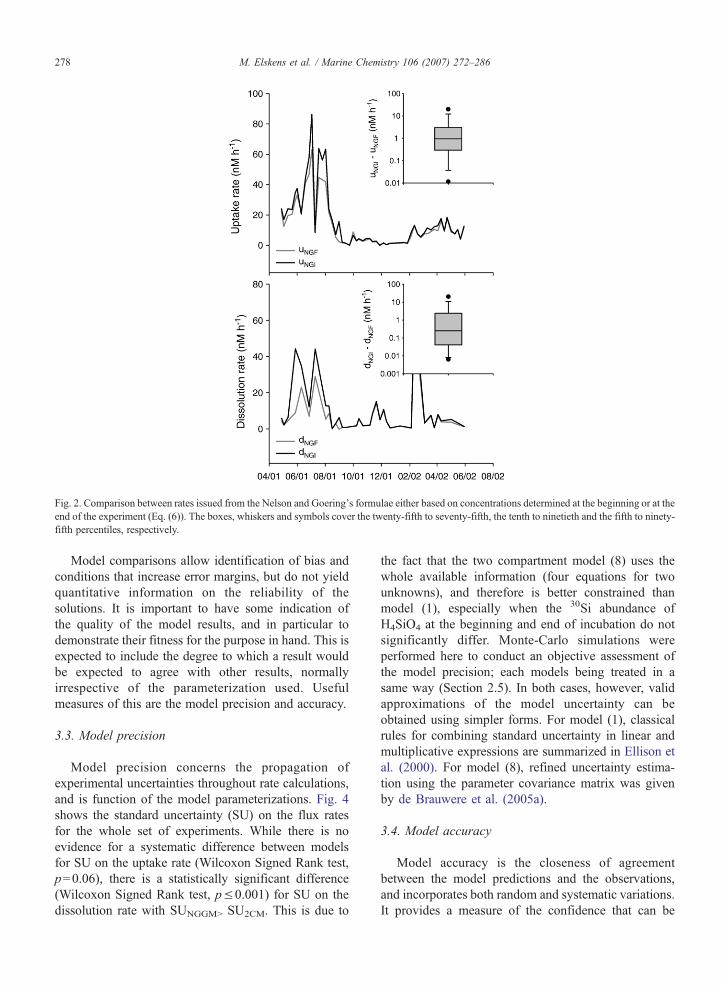
Fig. 2. Comparison between rates issued from the Nelson and Goering's formulae either based on concentrations determined at the beginning or at theend of the experiment (Eq. (6)). The boxes, whiskers and symbols cover the twenty-fifth to seventy-fifth, the tenth to ninetieth and the fifth to ninety-fifth percentiles, respectively.

278 M. Elskens et al. / Marine Chemistry 106 (2007) 272–286

Model comparisons allow identification of bias andconditions that increase error margins, but do not yieldquantitative information on the reliability of thesolutions. It is important to have some indication ofthe quality of the model results, and in particular todemonstrate their fitness for the purpose in hand. This isexpected to include the degree to which a result wouldbe expected to agree with other results, normallyirrespective of the parameterization used. Usefulmeasures of this are the model precision and accuracy.

3.3. Model precision

Model precision concerns the propagation ofexperimental uncertainties throughout rate calculations,and is function of the model parameterizations. Fig. 4shows the standard uncertainty (SU) on the flux ratesfor the whole set of experiments. While there is noevidence for a systematic difference between modelsfor SU on the uptake rate (Wilcoxon Signed Rank test,p=0.06), there is a statistically significant difference(Wilcoxon Signed Rank test, p≤0.001) for SU on thedissolution rate with SUNGGM> SU2CM. This is due to

the fact that the two compartment model (8) uses thewhole available information (four equations for twounknowns), and therefore is better constrained thanmodel (1), especially when the 30Si abundance ofH4SiO4 at the beginning and end of incubation do notsignificantly differ. Monte-Carlo simulations wereperformed here to conduct an objective assessment ofthe model precision; each models being treated in asame way (Section 2.5). In both cases, however, validapproximations of the model uncertainty can beobtained using simpler forms. For model (1), classicalrules for combining standard uncertainty in linear andmultiplicative expressions are summarized in Ellison etal. (2000). For model (8), refined uncertainty estima-tion using the parameter covariance matrix was givenby de Brauwere et al. (2005a).

3.4. Model accuracy

Model accuracy is the closeness of agreementbetween the model predictions and the observations,and incorporates both random and systematic variations.It provides a measure of the confidence that can be

Fig. 3. Comparison between rates issued from the upgrading formulae of Nelson and Goering (Eq. (7)) and the two compartmental model (Eq. (8)).The boxes, whiskers and symbols cover the twenty-fifth to seventy-fifth, the tenth to ninetieth and the fifth to ninety-fifth percentiles, respectively.

279M. Elskens et al. / Marine Chemistry 106 (2007) 272–286

placed on a model result. In order to test the modelaccuracy, we first utilized the standardized residualtechnique (Eq. (13)). For the upgraded Nelson andGoering's formulae (Eq. (7); Fig. 5a), the RSi-scores donot behave as standard normal variables. Rather, the

Fig. 4. Standard uncertainty (SU) on flux rates calculations for model (1) anddescribed in the text. Subscripts u and d stand for uptake and dissolution ratefifth, the tenth to ninetieth and the fifth to ninety-fifth percentiles, respective

distributions are skewed, medians mainly differ from 0,and there are too many unacceptable scores. Asdiscussed in the next section, a high score value canreflect an outlying measurement. Thought, when morethan 25% of the score distribution is >3, there are

model (8). SU-values were computed with Monte-Carlo simulations ass. The boxes, whiskers and symbols cover the twenty-fifth to seventy-ly.

Fig. 5. RSi-scores for models (1) and (8). (A) Upgraded Nelson and Goering's formulae, (B) Outcomes of the two compartment model. Absolutevalue of RSi>3 indicates unacceptably poor model performance in terms of accuracy while for a satisfactory performance |RSi|≤2 is required.The boxes, whiskers and symbols cover the twenty-fifth to seventy-fifth, the tenth to ninetieth and the fifth to ninety-fifth percentiles,respectively.

280 M. Elskens et al. / Marine Chemistry 106 (2007) 272–286

evidence for model failures as observed between Mayand September 2001. Under these conditions, thedifference between the model fits and measurements istoo high to be explained by random variations only. Onthe other hand, the RSi-scores for the two compartmentmodel better fit to the ideal zero-centred distribution(Fig. 5b): there is no evidence of systematic errors.

Some additional values were attached to methods ofcombining scores. For example the sum of the squaredstandardized residuals (Eq. (15)) yield an interpretablecost function CF, which behaves as a sample from a χ2

distribution. To check the overall statistical behaviour,our CF-values for model (8) were compared with the95–99% percentiles of the χ2 distribution. In addition,the CF-values were plotted in a histogram, which caneasily be compared with the probability density function(pdf) of the χ2 distribution (Fig. 6). Two observationscan be made:

(i) Two measurement sets produce a residual CFgreater than the 95th percentile, one of them being

even greater than the 99th percentile. Accordingto the Analytical Methods Committee (1992), thismeans that one result should be rejected(CF>χ299%) and the other one is questionable(χ295%<CF≤χ299%). From a statistical point ofview, instead of the expected 5 and 1% that exceedthe 95 and 99th percentiles, respectively, 4 and 2%do so. This is well acceptable since the 41measurements do not represent 41 realizations ofthe same experiment, but correspond to a one yeartime series. Therefore, the variability is not onlydue to random noise, but also to environmentalchanges.

(ii) Apart from these 2 experiments, it is also obviousin both pictures that most of the CF-values arevery close to zero. These extreme low valuescause a discrepancy between the histogram andthe pdf of the χ2 function. This is probably due toan overestimation of the experimental uncertain-ties. These latter were indeed used in the costfunction to weight the data, which results in a CF-value that is too small in case of overestimated

Fig. 6. Cost function values for the series of 53 experiments carried out by Beucher et al. (2004a). The histogram enables a comparison with the χ2

probability distribution function (pdf).

281M. Elskens et al. / Marine Chemistry 106 (2007) 272–286

residual variance (Eq. (14)). Fig. 5b suggests thatthese overestimations could affect the standarddeviations on H4SiO4 concentration and on 30Siat.%. For these measurements, the spread of theRSi distributions is too small. In well behavedsystems, the box (50% of the data) and the dots(95% of the data) should approximately extend to±1 and ±2, as reported for the RSi distribution ofBSiO2.

These observations have two main consequences.First, because the CF-value is probably underestimated,the chance of making a Type II error (accepting a wrongmodel result) increases. Secondly, by propagatingovervalued standard deviation through Monte-Carlosimulations, the standard uncertainty on the final modelresult is overestimated. These points illustrate well theimportance for correct estimations of measurementrepeatability as outlined by ISO guidelines.

3.5. Handling of outliers

Outliers are extreme observations that for one reasonor another do not belong to the other observations in thedataset. If the model equations are routinely applied tothese data, then the obtained estimates can be seriouslymisleading. Hereafter, we present a formal treatment fordetecting outliers with undue influence in parameterassessment and demonstrate the serious consequences offailing to detect outliers. The procedure combining theanalysis of standardized residuals and cost function is asfollows:

1. Optimize parameter-values with the two compart-mental model, and compare the residual CF-value to

the 99%-quantile of the χ2 distribution. If the modelfit is such that CF>χ299% go to 2.

2. Analyse the SRi-scores. If one absolute value of thescores is close to 3 - (the others being ≤1), remove it(it is an unusual observation with respect to theothers) and repeat step 1 with one degree of freedomless (n-p-1). If not go to 3.

3. If several absolute values of the scores are greaterthan 2, remove one by one (each time keeping theother outlying scores) repeating step 1 with onedegree of freedom less (n−p−1). Keep only thatmodel with the lowest CF-value. If not go to 4.

4. When discrimination between various residual CF-values is impossible (e.g. all the values are acceptableand close together), or when the residual costfunction remains greater than >χ299% after datatreatment, one cannot warrant the flux rate-values,and the results must be discarded.

In order to illustrate steps 2 to 4, we randomlygenerated outlying observations in the dataset no. 38 ofBeucher et al., 2004a. Under these conditions, thereference rates are known, and can be used to validatethe procedure. There are three issues for the interpreta-tion of this outlier simulation test (Table 1). First, inmost simulations, the CF-values (initial) lead to therejection of the model results (>χ299%) and the datawere subsequently processed according to steps 2 to 4.In the remaining part, the model results were question-able (χ295%<CF≤χ299%), which is not unusual enoughto justify further data treatments (e.g. Table 1, #11 and12). Second, the standardized residuals analysis hasrevealed in most cases an unusual score with respect tothe values of the others. This score was simply removedand the data processed according to step 2. In the

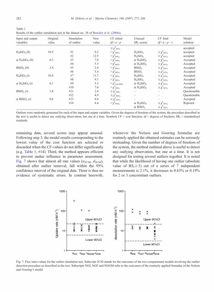
Table 1Results of the outlier simulation test in the dataset no. 38 of Beucher et al. (2004a)

Input and outputvariables

Originalvalue

Simulationof outlier

Newvalue

CF initialdf=n−p

UnusualSRi scores

CF finaldf=n−p−1

Modelsolution

≤χ295% acceptedH4SiO4 (0) 10.5 #1 9.2 >χ299% H4SiO4 ≤χ295% accepted

#2 12.5 >χ299% H4SiO4 ≤χ295% acceptedæ H4SiO4 (0) 6.3 #3 7.8 >χ299% æ H4SiO4 ≤χ295% Accepted

#4 5.5 >χ299% æ H4SiO4 ≤χ295% AcceptedBSiO2 (0) 3.4 #5 2.4 >χ299% BSiO2 ≤χ295% Accepted

#6 5.4 >χ299% BSiO2 ≤χ295% AcceptedH4SiO4 (t) 10.4 #7 11.7 >χ299% H4SiO4 ≤χ295% Accepted

#8 9.1 >χ299% H4SiO4 ≤χ295% Acceptedæ H4SiO4 (t) 6.1 #9 5.3 >χ2crit,99% æ H4SiO4 ≤χ295% Accepted

#10 7.6 >χ299% æ H4SiO4 ≤χ295% AcceptedBSiO2 (t) 3.8 #11 2.6 ≤χ299% – – Questionable

#12 4.9 ≤χ299% – – Questionableæ BSiO2 (t) 0.6 #13 0.4 ≤χ295% – – Accepted

#14 4.4 >χ299% æ H4SiO4 ≤χ295% Rejectedæ BSiO2 ≤χ295%

Outliers were randomly generated for each of the input and output variables. Given the degrees of freedom of the system, the procedure described inthe text is useful to detect any outlying observation, but one at a time. Symbols CF = cost function; df = degrees of freedom; SRi = standardizedresiduals.

282 M. Elskens et al. / Marine Chemistry 106 (2007) 272–286

remaining data, several scores may appear unusual.Following step 3, the model results corresponding to thelowest value of the cost function are selected ordiscarded when the CF-values do not differ significantly(e.g. Table 1, #14). Third, the method appears efficientto prevent undue influence in parameter assessment.Fig. 7 shows that almost all rate values (u2CM, d2CM),obtained after outlier removal, fall within the 95%confidence interval of the original data. There is thus noevidence of systematic errors. In contrast herewith,

Fig. 7. Flux rates-values for the outlier simulation test. Subscript 2CM standsdetection procedure as described in the text. Subscripts NGI, NGF and NGGMand Goering’s model.

whenever the Nelson and Goering formulae areroutinely applied the obtained estimates can be seriouslymisleading. Given the number of degrees of freedom ofthe system, the method outlined above is useful to detectany outlying observation, but one at a time. It is notdesigned for testing several outliers together. It is notedthat while the likelihood of having one outlier (absolutevalue of RSi≥3) out of a series of 7 independentmeasurements is 2.1%, it decreases to 0.63% or 0.19%for 2 or 3 concomitant outliers.

for the outcomes of the two compartment models involving the outlierrefer to the outcomes of the routinely applied formulae of the Nelson

Table 2Results of model selection (MS)

Batchexperiment

Date d nM/h u nM/h d nM/h u nM/h CF Index

Before MS After MS AR HL TA

1 28/04/01 6.0±1.4 22.2±1.1 6.0±1.4 22.2±1.1 sat GS GS 452 03/05/01 4.4±1.6 15.3±0.9 <MDL 15.7±1.1 que GS GS 323 12/05/01 5.6±1.2 20.8±1.2 5.6±1.2 20.8±1.2 sat GS GS 164 21/05/01 3.9±3.0 23.4±1.2 <MDL 22.5±1.6 sat GS GS 22 md5 28/05/01 20.2±1.9 50.6±2.6 20.2±1.9 50.6±2.6 sat 0.17 GS 196 01/06/01 11±3.4 38.9±4.0 <MDL 33.2±2.0 sat GS GS 53 md7 10/06/01 23.3±2.6 19±7 26.9±2.3 <MDL que GS GS 368 19/06/01 6.6±3.5 42.1±3.1 <MDL 37.5±2.4 sat GS GS 17 md9 27/06/01 10.5±1.7 46.3±2.2 10.5±1.7 46.3±2.2 sat GS GS 1810 03/07/01 34.7±6.9 84.6±7.6 34.7±6.9 84.6±7.6 sat GS 1.0 21 md11 10/07/01 27.0±3.6 38.9±4.5 27.0±3.6 38.9±4.5 sat GS 0.8 1512 18/07/01 25.8±4.8 54.8±4.7 25.8±4.8 54.8±4.7 sat GS GS 13 md13 26/07/01 13.9±2.1 45.2±3.2 13.9±2.1 45.2±3.2 sat GS GS 17 md14 02/08/01 6.9±1.0 23.7±2.7 6.9±1.0 23.7±2.7 sat 0.19 GS 2515 09/08/01 5.6±1.4 20.3±1.4 5.6±1.4 20.3±1.4 sat GS GS 1616 16/08/01 1.6±1.5 14.9±1.8 <MDL 15.3±1.9 sat GS GS 1117 24/08/01 1.6±1.9 6.3±1.1 <MDL 7.0±0.8 sat GS GS 1318 31/08/01 1.4±1.8 2.8±1.2 <MDL 3.6±0.5 sat GS GS GS19 07/09/01 1.7±1.3 0.7±1.1 <MDL 2.0±0.2 sat GS GS GS20 14/09/01 −0.1±1.6 1.5±0.9 <MDL 1.4±0.2 sat GS GS GS21 23/09/01 −4.9±2.2 2.1±1.4 −4.9±2.2 2.1±1.4 uns GS GS 1122 01/10/01 22.0±2.3 5.7±1.1 <MDL 6.4±0.8 sat GS GS 1323 08/10/01 2.5±2.1 1.9±1.1 <MDL 2.7±0.7 sat GS GS 1224 13/10/01 2.2±2.4 2.4±2.2 <MDL 4.2±0.9 sat GS GS GS25 22/10/01 −0.2±2.0 3.0±1.0 <MDL 3.0±0.4 sat GS GS 1326 29/10/01 1.5±1.1 1.2±2.2 1.9±1.0 <MDL sat GS GS GS27 06/11/01 −0.9±3.0 4.9±1.8 <MDL 4.4±0.5 sat GS GS 1128 12/11/01 3.9±2.4 0.8±1.4 4.4±2.5 <MDL sat GS GS 1329 20/11/01 2.2±2.8 1.8±1.4 <MDL 2.7±0.3 sat GS GS 1330 28/11/01 3.7±8.2 1.2±8.9 2.7±3.1 <MDL sat GS GS 1131 06/12/01 2.4±3.6 0.6±1.6 3.4±2.6 <MDL sat GS GS 11 md32 12/12/01 −0.5±3.7 0.7±1.7 <MDL 0.4±0.2 sat GS GS GS33 20/12/01 −2.0±2.2 2.1±1.1 <MDL 1.3±0.2 sat GS GS 1234 11/01/02 2.6±3.4 0.7±1.4 3.5±2.9 <MDL sat GS GS 1635 18/01/02 0.9±3.5 1.4±2.0 <MDL 1.9±0.5 sat GS GS GS36 27/01/02 −0.2±4.8 1.5±2.1 <MDL 1.4±1.2 sat GS GS 1137 04/02/02 3.4±5.9 6.6±3.5 <MDL 8.3±2.2 sat GS GS GS38 11/02/02 9.6±6.3 14.1±4.6 <MDL 14.3±2.7 sat GS GS GS39 18/02/02 0.5±10.1 7.6±5.8 <MDL 7.3±1.8 sat GS GS GS40 25/02/02 1.2±7.0 5.2±2.6 <MDL 5.6±1.3 sat GS GS 1441 05/03/02 3.0±5.9 7.4±2.3 <MDL 8.4±0.8 sat GS GS 1842 11/03/02 7.4±8.8 8.4±3.8 <MDL 11.3±1.0 sat GS GS 1843 19/03/02 3.2±4.6 9.0±1.8 <MDL 10.0±1.2 sat GS GS 1644 26/03/02 −1.0±4.5 12.5±2.0 <MDL 12.2±1.0 sat GS GS 2145 03/04/02 4.7±2.7 11.0±1.5 <MDL 12.6±1.1 sat GS GS 1846 10/04/02 1.4±2.0 16.7±2.0 <MDL 17.3±2.1 sat GS GS 1147 17/04/02 0.9±2.4 9.2±1.0 <MDL 9.5±0.9 sat GS GS 16 md48 23/04/02 2.3±2.7 18.1±1.2 <MDL 17.7±1.5 sat GS GS 18 md49 02/05/0 3.3±0.9 8.6±0.8 3.3±0.9 8.6±0.8 sat GS GS 1650 10/05/02 0.8±2.2 7.2±0.7 <MDL 7.4±0.7 sat GS GS 17 md51 16/05/02 4.6±2.2 8.9±1.2 <MDL 9.7±1.0 sat GS GS 14 md52 22/05/02 1.2±1.4 3.7±0.7 <MDL 4.0±0.5 GS GS 17 md53 30/05/02 0.9±1.4 11.4±1.9 <MDL 11.4±2.0 GS GS GS

Datasets from Beucher et al. (2004a). Symbols: CF = cost function, sat = satisfactory (CF≤χ295%), que = questionable (χ295%<CF≤χ299%), uns =unsatisfactory (CF>χ299%), MDL = model detection limit, AR = abundance ratio, HL = half-life of BSiO2, TA = tracer addition relative to the H4SiO4

ambient level (%), md = missing data, GS = good status for the index under consideration (AR≈1; HL≫1; TA≤10%).

283M. Elskens et al. / Marine Chemistry 106 (2007) 272–286

284 M. Elskens et al. / Marine Chemistry 106 (2007) 272–286

3.6. Reliability of the model solutions

When judged by the overall performance (precision,accuracy and robustness), model (1) clearly failed whencompared to Eq. (8). It should be noted, however, thatthe analytical solutions of Eq. (1) correspond to peculiarsolutions of Eq. (8) when u or d are equal to 0. Becausesuch conditions may occur, we do not reject Eq. (1) ingeneral but need a model selection strategy to decidewhen a parameter can be cancelled without losing theinformation hidden in the measurements. Put in anotherway, oversimplified models such as Eq. (1) risk biaswhen their underlying assumptions are violated, butoverly complex models such as Eq. (8) can misinterpretpart of the random noise as relevant processes.

To select optimal solutions subsets corresponding to agiven data set, we applied a procedure recently proposedby de Brauwere et al. (2005b), combining a statisticalinterpretation of the cost function and the principle ofparsimony. The approach provides a sound basis formodel selection because it is well recognized that otherthings being equal, the greater the number of parameters,the greater the extent of nonlinear behaviour, the worsethe model predictability (Ratkowsky, 1990). Theoptimized parameter values obtained after model selec-tion are shown in Table 2. Several remarks can be made:

(i) After selection, uptake and dissolution rates wererespectively removed from the model equations inrespectively 11 and 66% of the experiments. It isimportant to appreciate that this does not meanthat the rates equal zero, only that they cannot bereliably quantified. Hence they should be regardedas censored data (below the model detectionlimit).

(ii) The standard uncertainty on the remaining para-meters is mostly lower than before selection(Wilcoxon Signed Rank test, p≤0.001). This isone of the rewards using model selection: byreducing the number of parameters, the uncer-tainty on the remaining parameters decreases.

(iii) Rate values are given for the 12 datasets for whichthe 30Si abundance of H4SiO4 or/and BSiO2 wasmissing. This is allowed because with one missingdata, there is still one degree of freedom left (n−p−1) and the model is constrained.

Furthermore, Table 2 summarizes information on thevarious index types used to estimate the measurements,such as the abundance ratio (AR), the half-life of BSiO2

(HL) and the tracer addition (TA). Combined with the

CF approach, this information indicates which reliabilitycan be given to the final results.

4. Conclusions and final remarks

This paper provides advice on the concepts andpractices of quality assurance and quality control whenvalidating a model result. Whilst these guidelines wereillustrated with model results based on the 30Si tracermethodology, they have wider applications, e.g. tracerenrichment and dilution experiments.

It was emphasized that isotope enrichment anddilution models belong to a class of compartmentalmodels for which the governing law is mass conserva-tion. They are described by a set of differentialequations, and their structure is categorized as stochasticsince any variables in the model can be expressed by aprobability distribution. Therefore, estimating the modelparameters with a weighted least squares techniqueallows improving the accuracy of the parameter values,making them less sensitive to outlying observations.Standardized residuals that have normal distributions,and sum of the weighted least square residuals that haveχ2 distributions are matching techniques (easily inter-pretable with significance tests) for determining whethera model result is satisfactory or not. Additionally, thereare a number of analytical and experimental considera-tions on experimental design (abundance ratio, half-life,tracer addition indexes) and measurement uncertainty(repeatability of analytical methods), which are neededfor a correct model assessment. Combining theseapproaches with significance testing allows us tojudge the quality of the model results.

5. Glossary

Symbols

Definition Units

æ's

30Si at.% enrichment in the various Sicompartments or associated with thecorresponding flux rates as indicated by thesubscript

%

C

Concentration of the Si compartments μM BSiO2 Concentration of biogenic silica μM H4SiO4 Concentration of silicic acid μM ϕ Si flux rates μM h−1

u

Uptake rate of H4SiO4 μM h−1

d

Dissolution rate of BSiO2 μM h−1

(0, t)

Initial and final times of the incubation period h AR Abundance ratio index – HL Half-life index of BSiO2 – TA Tracer addition index % CF Cost function (=sum of the squared residuals) – fmodel(xi,ϕ) The ith model forecast μM or %

285M. Elskens et al. / Marine Chemistry 106 (2007) 272–286

n

The number of model equations – p The number of parameters to be

estimated in a given model

–

SRi

The standardized residual – SU The standard uncertainty μM/h xi The ith input variable μM or % yi The ith output variable μM or % σi Standard deviation of the ith residual – σx,j Standard deviation of the jth input variable μM or % σy,j Standard deviation of the jth ouput variable μM or % ∂yi/∂xj The partial differential of yi with respect to xj –

Acknowledgments

This paper is dedicated to the memory of RolandWollast, who guided the first steps of Marc Elskens inIGBP and Global Change related Research in Belgium(1989–95). This research was conducted under grantGOA22/DSCHWER4 as part of the project Geconcer-teerde Onderzoekacties supported by the Vrije Uni-versiteit Brussel.

References

Analytical Methods Committee, 1992. Proficiency testing of analyticallaboratories: organization and statistical assessment. Analyst 117,97–117.

Beucher, C., Tréguer, P., Corvaisier, R., Hapette, A.-M., Elskens, M.,2004a. Production and dissolution of biogenic silica in a coastalecosystem of western Europe. Marine Ecology Progress Series267, 57–69.

Beucher, C., Tréguer, P., Corvaisier, R., Hapette, A.-M., Pichon, J.-J.,Metzl, N., 2004b. Intense summer biosilica recycling in theSouthern Ocean. Geophysical Research Letters 31. doi:10.1029/2003GL.018998.

Bidle, K.D., Azam, F., 1999. Accelerated dissolution of diatom silicaby marine bacterial assemblages. Nature 397, 508–512.

Box, M.J., 1970. Improved parameter estimation. Technometrics 12,219–229.

Brzezinski, M.A., Phillips, D.R., 1997. Evaluation of Si-32 as a tracerfor measuring silica production rates in marine waters. Limnologyand Oceanography 42, 856–865.

Brzezinski, M.A., Villareal, T.A., Lipschultz, F., 1998. Silicaproduction and the contribution of diatoms to new and primaryproduction in the central North Pacific. Marine Ecology ProgressSeries 167, 89–104.

Collos, Y., 1987. Calculations of 15N uptake rates by phytoplanktonassimilating one or several nitrogen sources. Applied Radiationand Isotopes 38, 275–282.

Collos, Y., Slawyk, G., 1985. On The compatibility of carbon uptakerates calculated from stable and radioactive isotope data —implications for the design of experimental protocols inaquatic primary productivity. Journal of Plankton Research 7,595–603.

Corvaisier, R., Tréguer, P., Beucher, C., Elskens, M., 2005.Determination of the rate of production and dissolution of biosilicain marine waters by thermal ionisation mass spectrometry.Analytica Chemica Acta 534, 149–155.

de Brauwere, A., De Ridder, F., Elskens, M., Schoukens, J., Pintelon,R., Baeyens, W., 2005a. Refined parameter and uncertaintyestimation when both variables are subject to error. Case study:estimation of Si consumption and regeneration rates in a marineenvironment. Journal of Marine Systems 55, 205–221.

de Brauwere, A., De Ridder, F., Pintelon, R., Elskens, M., Schoukens,J., Baeyens, W., 2005b. Model selection through a statisticalanalysis of the minimumof aWeighted Least Squares cost function.Chemometrics and Intelligent Laboratory Systems 76, 163–173.

De La Rocha, C.L., Brzezinski, M.A., De Niro, M.J., 1997.Fractionation of silicon isotopes by marine diatoms duringbiogenic silica formation. Geochimica et Cosmochimica Acta 61(23), 5051–5056.

Dugdale, R.C., Goering, J.J., 1967. Uptake of new and regeneratedforms of nitrogen in primary productivity. Limnology andOceanography 12, 196–206.

Dugdale, R.C., Wilkerson, F.P., 1986. The use of 15N to measurenitrogen uptake in eutrophic oceans; experimental considerations.Limnology and Oceanography 31, 673–689.

Ellison, S.L.R., Rosslein, M., William, A. (Eds.), 2000. QuantifyingUncertainty in Analytical Measurement, EURACHEM/CITACGuide CG4. UK Dep. of Trade and Ind., London. 120 pp.

Elskens, M., Baeyens, W., Brion, N., De Galan, S., Goeyens, L., deBrauwere, A., 2005. Reliability of n flux rates estimated from 15Nenrichment and dilution experiments in aquatic systems, GlobalBiogeochemical Cycles 19, GB4028.

Goering, J.J., Nelson, D.M., Carter, J.A., 1973. Silicic acid uptake bynatural populations of marine phytoplankton. Deep-Sea Research20, 777–789.

Harrison, W., 1983. Nitrogen in the marine environment: Use ofisotopes. In: Carpenter, E.J., Capone, D.G. (Eds.), Nitrogen in theMarine Environment. Academic Press, Inc., pp. 763–808.

Horwitz, W., 1983. Today's chemical realities. Journal of AOACInternational 66, 1295–1301.

Janssen, P.H.M., Heuberger, P.S.C., 1995. Calibration of process-oriented models. Ecological Modelling 83, 55–66.

Klemens, P., Heumann, K.G., 2001. Development of an ICP-HRIDMSmethod for accurate determination of traces of silicon in biologicaland clinical samples. Fresenius' Journal of Analytical Chemistry371, 758–763.

Legendre, L., Gosselin, M., 1996. Estimation of N or C uptake rates byphytoplankton using 15N or 13C: revisiting the usual computationformulae. Journal of Plankton Research 19, 263–271.

Nelson, D.M., Goering, J.J., 1977a. A stable Isotope Tracer Method toMeasure Silicic Acid Uptake by Marine Phytoplankton. AnalyticalBiochemistry 78, 139–147.

Nelson, D.M., Goering, J.J., 1977b. Near-surface silica dissolution inthe upwelling region off northwest Africa. Deep-Sea Research 24,65–73.

Nelson, D.M., Gordon, L.I., 1982. Production and pelagic dissolutionof biogenic silica in the Southern Ocean. Geochimica etCosmochimica Acta 46, 491–500.

Nelson, D.M., Ahern, J.A., Herlihy, L.J., 1991. Cycling of biogenicsilica within the upper water column of the Ross Sea. MarineChemistry 45, 461–476.

Quéguiner, B., 2001. Biogenic silica production in theAustralian sector of the Sub-Antartic Zone of the southern Oceanin late summer 1998. Journal of Geophysical Research 106,31627–31636.

Ragueneau, O., Tréguer, P., 1994. Determination of biogenic silica incoastal waters — applicability and limits of the alkaline digestionmethod. Marine Chemistry 45, 43–51.

286 M. Elskens et al. / Marine Chemistry 106 (2007) 272–286

Ratkowsky, D.A., 1990. Handbook of nonlinear regression models. In:Owen, D.B. (Ed.), Statistics: textbooks and Monographs. MarcelDekker, INC, New York. ISBN: 0-8247-8189-9, p. 241.

Rod, V., Hancil, V., 1980. Iterative estimation of model parameterswhen measurements of all variables are subject to error. Computers& Chemical Engineering 4, 33–38.

Strickland, J.D.H., Parsons, T.R., 1968. A practical handbook ofsweater analysis. In: Stevenson, J.C. (Ed.), Fisheries ResearchBoard of Canada. Bulletin, vol. 167, p. 311.

Thompson, M., Lowthian, P.J., 1997. The Horwitz function revisited.Journal of AOAC International 80, 676–679.

Tréguer, P., Lindner, L., Vanbennekom, A.J., Leynaert, A., Panouse,M., Jacques, G., 1991. Production of biogenic silica in theWeddell–Scotia Seas measured with Si-32. Limnology andOceanography 36, 1217–1227.