Statistical Outlier Detection Using Direct Density … Outlier Detection Using Direct Density Ratio...
35
1 Knowledge and Information Systems. vol.26, no.2, pp.309-336, 2011. Statistical Outlier Detection Using Direct Density Ratio Estimation Shohei Hido IBM Research, Tokyo Research Laboratory, Japan. Department of Systems Science, Kyoto University, Japan [email protected] Yuta Tsuboi IBM Research, Tokyo Research Laboratory, Japan. [email protected] Hisashi Kashima ∗ IBM Research, Tokyo Research Laboratory, Japan. [email protected] Masashi Sugiyama Department of Computer Science, Tokyo Institute of Technology, Japan. PRESTO, Japan Science and Technology Agency, Japan. [email protected] http://sugiyama-www.cs.titech.ac.jp/˜sugi Takafumi Kanamori Department of Computer Science and Mathematics Informatics, Nagoya University, Japan. [email protected] Abstract We propose a new statistical approach to the problem of inlier-based outlier detec- tion, i.e., finding outliers in the test set based on the training set consisting only of inliers. Our key idea is to use the ratio of training and test data densities as an outlier score. This approach is expected to have better performance even in high-dimensional problems since methods for directly estimating the density ratio without going through density estimation are available. Among various density ra- tio estimation methods, we employ the method called unconstrained least-squares importance fitting (uLSIF) since it is equipped with natural cross-validation proce- dures, allowing us to objectively optimize the value of tuning parameters such as the regularization parameter and the kernel width. Furthermore, uLSIF offers a closed-form solution as well as a closed-form formula for the leave-one-out error, so * Currently with Department of Mathematical Informatics, The University of Tokyo, Japan.
Transcript of Statistical Outlier Detection Using Direct Density … Outlier Detection Using Direct Density Ratio...

1Knowledge and Information Systems. vol.26, no.2, pp.309-336, 2011.
Statistical Outlier DetectionUsing Direct Density Ratio Estimation
Shohei HidoIBM Research, Tokyo Research Laboratory, Japan.
Department of Systems Science, Kyoto University, [email protected]
Yuta TsuboiIBM Research, Tokyo Research Laboratory, Japan.
Hisashi Kashima∗
IBM Research, Tokyo Research Laboratory, [email protected]
Masashi SugiyamaDepartment of Computer Science, Tokyo Institute of Technology, Japan.
PRESTO, Japan Science and Technology Agency, [email protected] http://sugiyama-www.cs.titech.ac.jp/˜sugi
Takafumi KanamoriDepartment of Computer Science and Mathematics Informatics,
Nagoya University, [email protected]
Abstract
We propose a new statistical approach to the problem of inlier-based outlier detec-tion, i.e., finding outliers in the test set based on the training set consisting onlyof inliers. Our key idea is to use the ratio of training and test data densities asan outlier score. This approach is expected to have better performance even inhigh-dimensional problems since methods for directly estimating the density ratiowithout going through density estimation are available. Among various density ra-tio estimation methods, we employ the method called unconstrained least-squaresimportance fitting (uLSIF) since it is equipped with natural cross-validation proce-dures, allowing us to objectively optimize the value of tuning parameters such asthe regularization parameter and the kernel width. Furthermore, uLSIF offers aclosed-form solution as well as a closed-form formula for the leave-one-out error, so
∗Currently with Department of Mathematical Informatics, The University of Tokyo, Japan.

Statistical Outlier Detection Using Direct Density Ratio Estimation 2
it is computationally very efficient and is scalable to massive datasets. Simulationswith benchmark and real-world datasets illustrate the usefulness of the proposedapproach.
Keywords
outlier detection, density ratio, importance, unconstrained least-squares importancefitting (uLSIF).
1 Introduction
The goal of outlier detection (a.k.a. anomaly detection, novelty detection, or one-class clas-sification) is to find uncommon instances (‘outliers’) in a given dataset. Outlier detectionhas been used in various applications such as defect detection from behavior patterns ofindustrial machines (Fujimaki, Yairi and Machida, 2005; Ide and Kashima, 2004), intru-sion detection in network systems (Yamanishi, Takeuchi, Williams and Milne, 2004), andtopic detection in news documents (Manevitz and Yousef, 2002). Recent studies includefinding unusual patterns in time-series (Yankov, Keogh and Rebbapragada, 2008), discov-ery of spatio-temporal changes in time-evolving graphs (Chan, Bailey and Leckie, 2008),self-propagating worm detection in information systems (Jiang and Zhu, 2009), and iden-tification of inconsistent records in construction equipment data (Fan, Zaıane, Foss andWu, 2009). Since outlier detection is useful in various applications it has been a ac-tive research topic in statistics, machine learning, and data mining communities fordecades (Hodge and Austin, 2004).
A standard outlier detection problem falls into the category of unsupervised learningdue to lack of prior knowledge on the ‘anomalous data’. In contrast, Gao, Cheng andTan (2006a) and Gao, Cheng and Tan (2006b) addressed the problem of semi-supervisedoutlier detection where some examples of outlier and inlier are available as a training set.The semi-supervised outlier detection methods could perform better than unsupervisedmethods thanks to additional label information, but such outlier samples for training arenot always available in practice. Furthermore, the type of outliers may be diverse and thusthe semi-supervised methods—learning from known types of outliers—are not necessarilyuseful in detecting unknown types of outliers.
In this paper, we address the problem of inlier-based outlier detection where examplesof inlier are available. More formally, the inlier-based outlier detection problem is tofind outlier instances in the test set based on the training set consisting only of inlierinstances. The setting of inlier-based outlier detection would be more practical than thesemi-supervised setting since inlier samples are often available abundantly. For example,in defect detection of industrial machines, we already know that there is no outlier (i.e.,a defect) in the past since no failure has been observed in the machinery. Therefore, it isreasonable to separate the measurement data into a training set consisting only of inliersamples observed in the past and the test set consisting of recent samples from which wetry to find outliers.

Statistical Outlier Detection Using Direct Density Ratio Estimation 3
As opposed to supervised learning, the outlier detection problem is vague and it is notpossible to universally define what the outliers are. In this paper, we consider a statisticalframework and regard instances with low probability densities as outliers. In light ofinlier-based outlier detection, outliers may be identified via density estimation of inliersamples. However, density estimation is known to be a hard problem particularly in highdimensions, so outlier detection via density estimation may not work well in practice.
To avoid density estimation, we may use One-class Support Vector Machine (OSVM)(Scholkopf, Platt, Shawe-Taylor, Smola and Williamson, 2001) or Support Vector DataDescription (SVDD) (Tax and Duin, 2004), which finds an inlier region containing acertain fraction of training instances; samples outside the inlier region are regarded asoutliers. However, these methods cannot make use of inlier information available in theinlier-based settings. Furthermore, the solutions of OSVM and SVDD depend heavily onthe choice of tuning parameters (e.g., the Gaussian kernel width) and there seems to beno reasonable method to appropriately determine the values of the tuning parameters.
To overcome the weakness of the existing methods, we propose a new approachto inlier-based outlier detection. Our key idea is not to directly model the trainingand test data densities, but only to estimate the ratio of training and test data den-sities. Among existing methods of density ratio estimation (Qin, 1998; Cheng andChu, 2004; Huang, Smola, Gretton, Borgwardt and Scholkopf, 2007; Bickel, Bruckner andScheffer, 2007; Sugiyama, Nakajima, Kashima, von Bunau and Kawanabe, 2008; Nguyen,Wainwright and Jordan, 2008; Sugiyama, Suzuki, Nakajima, Kashima, von Bunauand Kawanabe, 2008; Kanamori, Hido and Sugiyama, 2009a; Kanamori, Hido andSugiyama, 2009b), we employ an algorithm called unconstrained Least-Squares Impor-tance Fitting (uLSIF) (Kanamori, Hido and Sugiyama, 2009a; Kanamori, Hido andSugiyama, 2009b) for outlier detection. The reason for this choice is that uLSIF isequipped with a variant of cross-validation (CV), so the values of tuning parameters suchas the regularization parameter can be objectively determined without subjective trialand error. Furthermore, uLSIF-based outlier detection allows us to compute the out-lier score just by solving a system of linear equations—the leave-one-out cross-validation(LOOCV) error can also be computed analytically. Thus, uLSIF-based outlier detectionis computationally very efficient and therefore is scalable to massive datasets. Throughexperiments using benchmark datasets and real-world datasets of failure detection in harddisk drives and financial risk management in loan business, our approach is shown to com-pare favorably with existing outlier detection methods and other density ratio estimationmethods both in accuracy and scalability.
This paper is an extended version of our earlier conference paper presented at IEEEICDM 2008 (Hido, Tsuboi, Kashima, Sugiyama and Kanamori, 2008), with more detailsand additional results. The rest of this paper is organized as follows. In Section 2, wemathematically formulate the inlier-based outlier detection problem as a density ratioestimation problem. In Section 3, we give a comprehensive review of existing densityratio estimation methods. In Section 4, we discuss the characteristics of the existingdensity ratio estimation methods and propose a practical outlier detection procedure basedon uLSIF; illustrative numerical examples of the proposed method are also shown. In

Statistical Outlier Detection Using Direct Density Ratio Estimation 4
Section 5, we discuss the relation between the proposed uLSIF-based method and existingoutlier detection methods. In Section 6, we experimentally compare the performance ofthe proposed and existing algorithms using benchmark and real-world datasets. Finally,in Section 7, we conclude by summarizing our contributions.
2 Outlier Detection via Direct Importance Estima-
tion
In this section, we propose a new statistical approach to outlier detection.Suppose we have two sets of samples—training samples {xtr
j }ntrj=1 and test samples
{xtei }nte
i=1 in a domain D (⊂ Rd). The training samples {xtrj }ntr
j=1 are all inliers, while thetest samples {xte
i }ntei=1 can contain some outliers. The goal of outlier detection here is to
identify outliers in the test set based on the training set consisting only of inliers. Moreformally, we want to assign a suitable inlier score for the test samples—the smaller thevalue of the inlier score is, the more plausible the sample is an outlier.
Let us consider a statistical framework of the inlier-based outlier detection problem:suppose training samples {xtr
j }ntrj=1 are independent and identically distributed (i.i.d.) fol-
lowing a training data distribution with density ptr(x) and test samples {xtei }nte
i=1 arei.i.d. following a test data distribution with strictly positive density pte(x). Within thisstatistical framework, test samples with low training data densities are regarded as out-liers. However, ptr(x) is not accessible in practice and density estimation is known to bea hard problem. Therefore, merely using the training data density as an inlier score maynot be promising in practice.
In this paper, we propose to use the ratio of training and test data densities, calledthe importance, as an inlier score:
w(x) =ptr(x)
pte(x).
If there exists no outlier sample in the test set (i.e., the training and test data densitiesare equivalent), the value of the importance is one. The importance value tends to besmall in the regions where the training data density is low and the test data density ishigh. Thus samples with small importance values are plausible to be outliers.
One may suspect that this importance-based approach is not suitable when thereexist only a small number of outliers—since a small number of outliers cannot increasethe values of pte(x) significantly. However, outliers are drawn from a region with smallptr(x) and therefore a small change in pte(x) significantly reduces the importance value.For example, let the increase of pte(x) be ϵ = 0.01; then 1
1+ϵ≈ 1, but 0.001
0.001+ϵ≪ 1.
Thus the importance w(x) would be a suitable inlier score (see Section 4.3 for illustrativeexamples).

Statistical Outlier Detection Using Direct Density Ratio Estimation 5
3 Direct Importance Estimation Methods
The values of the importance are unknown in practice, so we need to estimate themfrom data samples. If one estimates the training and test densities separately from thedata samples, one will be able to estimate the importance just by taking the ratio ofthe two estimated densities. However, this naive approach can easily suffer from thecurse of dimensionality, particularly when the data has neither low dimensionality nor asimple distribution. As advocated by Vapnik (1998), density ratio estimation is crucialin statistical learning, but often unnecessarily more difficult than the target problem thatone would like to solve. In our case, we would like to directly estimate the importancevalues without going through density estimation. In this section, we review such directimportance estimation methods which could be used for inlier-based outlier detection. Infact, it has been shown that direction estimation methods work better than the two-stepapproach of separately estimating the two densities and then taking their ratio (Sugiyama,Suzuki, Nakajima, Kashima, von Bunau and Kawanabe, 2008). Therefore these methodsare expected to also work well on the inlier-based outlier detection problems.
3.1 Kernel Mean Matching (KMM)
The KMM method (Huang et al., 2007) avoids density estimation and directly gives anestimate of the importance at test points (i.e., data points drawn from the denominatorof the ratio).
The basic idea of KMM is to find w(x) such that the mean discrepancy betweennonlinearly transformed samples drawn from ptr(x) and pte(x) is minimized in a universalreproducing kernel Hilbert space (Steinwart, 2001). The Gaussian kernel
Kσ(x,x′) = exp
(−∥x− x′∥2
2σ2
)(1)
is an example of kernels that induce a universal reproducing kernel Hilbert space. It hasbeen shown that the solution of the following optimization problem agrees with the trueimportance:
minw
∥∥∥∥∫ Kσ(x, ·)ptr(x)dx−∫
Kσ(x, ·)w(x)pte(x)dx∥∥∥∥2F
s.t.
∫w(x)pte(x)dx = 1 and w(x) ≥ 0,
where ∥ · ∥F denotes the norm in the Gaussian reproducing kernel Hilbert space.An empirical version of the above problem is reduced to the following quadratic pro-
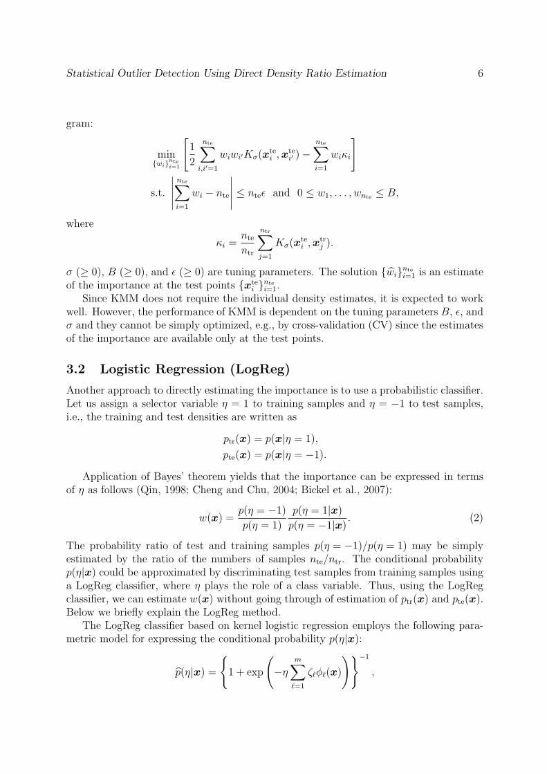
Statistical Outlier Detection Using Direct Density Ratio Estimation 6
gram:
min{wi}
ntei=1
[1
2
nte∑i,i′=1
wiwi′Kσ(xtei ,x
tei′ )−
nte∑i=1
wiκi
]
s.t.
∣∣∣∣∣nte∑i=1
wi − nte
∣∣∣∣∣ ≤ nteϵ and 0 ≤ w1, . . . , wnte ≤ B,
where
κi =nte
ntr
ntr∑j=1
Kσ(xtei ,x
trj ).
σ (≥ 0), B (≥ 0), and ϵ (≥ 0) are tuning parameters. The solution {wi}ntei=1 is an estimate
of the importance at the test points {xtei }nte
i=1.Since KMM does not require the individual density estimates, it is expected to work
well. However, the performance of KMM is dependent on the tuning parameters B, ϵ, andσ and they cannot be simply optimized, e.g., by cross-validation (CV) since the estimatesof the importance are available only at the test points.
3.2 Logistic Regression (LogReg)
Another approach to directly estimating the importance is to use a probabilistic classifier.Let us assign a selector variable η = 1 to training samples and η = −1 to test samples,i.e., the training and test densities are written as
ptr(x) = p(x|η = 1),
pte(x) = p(x|η = −1).
Application of Bayes’ theorem yields that the importance can be expressed in termsof η as follows (Qin, 1998; Cheng and Chu, 2004; Bickel et al., 2007):
w(x) =p(η = −1)p(η = 1)
p(η = 1|x)p(η = −1|x)
. (2)
The probability ratio of test and training samples p(η = −1)/p(η = 1) may be simplyestimated by the ratio of the numbers of samples nte/ntr. The conditional probabilityp(η|x) could be approximated by discriminating test samples from training samples usinga LogReg classifier, where η plays the role of a class variable. Thus, using the LogRegclassifier, we can estimate w(x) without going through of estimation of ptr(x) and pte(x).Below we briefly explain the LogReg method.
The LogReg classifier based on kernel logistic regression employs the following para-metric model for expressing the conditional probability p(η|x):
p(η|x) =
{1 + exp
(−η
m∑ℓ=1
ζℓϕℓ(x)
)}−1
,

Statistical Outlier Detection Using Direct Density Ratio Estimation 7
where m is the number of basis functions and {ϕℓ(x)}mℓ=1 are fixed basis functions. Bysubstituting this equation into Eq.(2), an importance estimator is given by
w(x) =p(η = −1)p(η = 1)
p(η = 1|x)p(η = −1|x)
=nte
ntr
1 + exp (∑m
ℓ=1 ζℓϕℓ(x))
1 + exp (−∑m
ℓ=1 ζℓϕℓ(x))
=nte
ntr
exp
(m∑ℓ=1
ζℓϕℓ(x)
).
The parameters {ζℓ}mℓ=1 are learned by minimizing the negative regularized log-likelihood:
minζ
[nte∑i=1
log
(1 + exp
(m∑ℓ=1
ζℓϕℓ(xtei )
))
+ntr∑j=1
log
(1 + exp
(−
m∑ℓ=1
ζℓϕℓ(xtr)
))+ λ
m∑ℓ=1
ζ2ℓ
].
Since the above objective function is convex, the global optimal solution can be obtainedby standard nonlinear optimization methods such as Newton’s method, conjugate gradi-ent, and the BFGS method (Minka, 2007).
An advantage of the LogReg method is that model selection (i.e., the choice of basisfunctions {ϕℓ(x)}mℓ=1 as well as the regularization parameter λ) is possible by standard CVsince the learning problem involved above is a standard supervised classification problem.
3.3 Kullback-Leibler Importance Estimation Procedure(KLIEP)
KLIEP (Sugiyama, Nakajima, Kashima, von Bunau and Kawanabe, 2008; Sugiyama,Suzuki, Nakajima, Kashima, von Bunau and Kawanabe, 2008) also directly gives an esti-mate of the importance function without going through density estimation by implicitlymatching the true and estimated distributions under the Kullback-Leibler divergence.
Let us model the importance w(x) by the following linear model:
w(x) =b∑
ℓ=1
αℓφℓ(x), (3)
where {αℓ}bℓ=1 are parameters and {φℓ(x)}bℓ=1 are basis functions such that φℓ(x) ≥ 0 forall x ∈ D and for ℓ = 1, . . . , b. Then an estimator of the training data density ptr(x) isgiven by
ptr(x) = w(x)pte(x).
In KLIEP, the parameters {αℓ}bℓ=1 are determined so that the Kullback-Leibler divergence

Statistical Outlier Detection Using Direct Density Ratio Estimation 8
from ptr(x) to ptr(x) is minimized:
KL[ptr(x)∥ptr(x)] =∫
ptr(x) logptr(x)
w(x)pte(x)dx
=
∫ptr(x) log
ptr(x)
pte(x)dx−
∫ptr(x) log w(x)dx. (4)
The first term is a constant, so it can be safely ignored. Since ptr(x) (= w(x)pte(x)) is aprobability density function, it should satisfy
1 =
∫ptr(x)dx =
∫w(x)pte(x)dx. (5)
The KLIEP optimization problem is then given by replacing the expectations in Eqs.(4)and (5) with empirical averages:
max{αℓ}bℓ=1
[ntr∑j=1
log
(b∑
ℓ=1
αℓφℓ(xtrj )
)]
s.t.1
nte
b∑ℓ=1
αℓ
(nte∑i=1
φℓ(xtei )
)= 1 and α1, . . . , αb ≥ 0.
This is a convex optimization problem and the global solution can be obtained, e.g., bysimply performing gradient ascent and feasibility satisfaction iteratively. A pseudo codeof the KLIEP optimization procedure is described in Figure 1. Note that the solution{αℓ}bℓ=1 tends to be sparse (Boyd and Vandenberghe, 2004), which contributes to reducingthe computational cost in the test phase. See Nguyen et al. (2008) and Sugiyama, Suzuki,Nakajima, Kashima, von Bunau and Kawanabe (2008) for the convergence proofs.
Model selection of KLIEP is possible by a variant of likelihood cross-validation (LCV)(Hardle, Muller, Sperlich and Werwatz, 2004) as follows. We first divide the trainingsamples {xtr
j }ntrj=1 into a learning part and a validation part, the model is trained based on
the learning part, and then its likelihood is verified using the validation part; the modelwith the largest estimated likelihood is chosen. A pseudo code of LCV for KLIEP isdescribed in Figure 2. Note that this LCV procedure corresponds to choosing the modelwith the smallest KL[ptr(x)∥ptr(x)].
A MATLAB R⃝ implementation of the entire KLIEP algorithm is available from thefollowing web page:
http://sugiyama-www.cs.titech.ac.jp/~sugi/software/KLIEP/
3.4 Least-squares Importance Fitting
KLIEP employed the Kullback-Leibler divergence for measuring the discrepancy betweentwo densities. Least-squares importance fitting (LSIF) (Kanamori, Hido and Sugiyama,

Statistical Outlier Detection Using Direct Density Ratio Estimation 9
Input: m = {φℓ(x)}bℓ=1, {xtrj }ntr
j=1, {xtei }nte
i=1
Output: w(x)
Aj,ℓ ←− φℓ(xtrj ) for j = 1, . . . , ntr and ℓ = 1, . . . , b;
bℓ ←− 1nte
∑nte
i=1 φℓ(xtei )
Initialize α = (α1, . . . , αb)⊤ (> 0) and ε (0 < ε≪ 1);
Repeat until convergenceα←− α+ εA⊤(1./Aα); % Gradient ascent
α←− α+ (1− b⊤α)b/(b⊤b);α←− max(0,α);
α←− α/(b⊤α);end
w(x)←−∑b
ℓ=1 αℓφℓ(x);
Figure 1: Pseudo code of the optimization procedure for KLIEP. 0 and 1 denote thevectors with all zeros and ones, respectively. ‘./’ indicates the element-wise division and⊤ denotes the transpose. Inequalities and the ‘max’ operation for vectors are applied inthe element-wise manner.
Input: M = {m = {φmℓ (x)}
bmℓ=1}, {xtr
j }ntrj=1, {xte
i }ntei=1
Output: w(x)
Split {xtrj }ntr
j=1 into R disjoint subsets {Xr}Rr=1;for each model m ∈M
for each split r = 1, . . . , Rwr(x)←− KLIEP(m, {xte
i }ntei=1, {Xj}j =r);
Jr(m)←− 1|Xr|∑
x∈Xrlog wr(x);
end
J(m)←− 1R
∑Rr=1 Jr(m);
end
m←− argmaxm∈M J(m);w(x)←− KLIEP(m, {xtr
j }ntrj=1, {xte
i }ntei=1);
Figure 2: Pseudo code of model selection for KLIEP by LCV.

Statistical Outlier Detection Using Direct Density Ratio Estimation 10
2009a; Kanamori, Hido and Sugiyama, 2009b) uses the squared loss for density-ratiofunction fitting. The density ratio w(x) is again modeled by the linear model (3).
The parameters {αℓ}bℓ=1 in the model w(x) are determined so that the followingsquared error J0 is minimized:
J0(α) =1
2
∫(w(x)− w(x))2 pte(x)dx
=1
2
∫w(x)2pte(x)dx−
∫w(x)ptr(x)dx+
1
2
∫w(x)ptr(x)dx, (6)
where the last term is a constant and therefore can be safely ignored. Let us denote thefirst two terms by J :
J(α) =1
2
∫w(x)2pte(x)dx−
∫w(x)ptr(x)dx.
Approximating the expectations in J by empirical averages, we obtain
J(α) =1
2nte
nte∑i=1
w(xtei )
2 − 1
ntr
ntr∑j=1
w(xtrj )
=1
2
b∑ℓ,ℓ′=1
αℓαℓ′Hℓ,ℓ′ −b∑
ℓ=1
αℓhℓ, (7)
where
Hℓ,ℓ′ =1
nte
nte∑i=1
φℓ(xtei )φℓ′(x
tei ), (8)
hℓ =1
ntr
ntr∑j=1
φℓ(xtrj ). (9)
Taking into account the non-negativity of the density-ratio function w(x), the optimiza-tion problem is formulated as follows.
min{αℓ}bℓ=1
[1
2
b∑ℓ,ℓ′=1
αℓαℓ′Hℓ,ℓ′ −b∑
ℓ=1
αℓhℓ + λb∑
ℓ=1
αℓ
]s.t. α1, . . . , αb ≥ 0, (10)
where a penalty term λ∑b
ℓ=1 αℓ is included for regularization purposes with λ (≥ 0)being a regularization parameter. Eq.(10) is a convex quadratic programming problemand therefore the unique global optimal solution can be computed efficiently by a standardoptimization package.
Model selection of the Gaussian width σ and the regularization parameter λ is possi-ble by a variant of CV: First, {xte
i }ntei=1 and {xtr
j }ntrj=1 are divided into R disjoint subsets

Statistical Outlier Detection Using Direct Density Ratio Estimation 11
Input: H and h % see Eqs.(8) and (9) for the definitionOutput: entire regularization path α(λ) for λ ≥ 0
τ ←− 0; k ←− argmaxi{hi | i = 1, . . . , b};λτ ←− hk; A ←− {1, . . . , b}\{k};α(λτ )←− 0b; % the vector with all zerosWhile λτ > 0
E ←− O|A|×b; % the matrix with all zeros
For i = 1, . . . , |A|Ei,ji ←− 1; % A = {j1, . . . , j|A| | j1 < · · · < j|A|}
end
G←−
(H −E
⊤
−E O|A|×|A|
);
u←− G−1
(h0|A|
); v ←− G
−1(
1b
0|A|
);
If v ≤ 0b+|A| % the final interval
λτ+1 ←− 0; α(λτ+1)←− (u1, . . . , ub)⊤;
else % an intermediate interval
k ←− argmaxi{ui/vi | vi > 0, i = 1, . . . , b+ |A|};λτ+1 ←− max{0, uk/vk};α(λτ+1)←− (u1, . . . , ub)
⊤ − λτ+1(v1, . . . , vb)⊤;
If 1 ≤ k ≤ b
A ←− A ∪ {k};else
A ←− A\{jk−b};end
endτ ←− τ + 1;
end
α(λ)←−
{0b if λ ≥ λ0λτ+1−λλτ+1−λτ
α(λτ ) +λ−λτ
λτ+1−λτα(λτ+1) if λτ+1 ≤ λ ≤ λτ
Figure 3: Pseudo code for computing the entire regularization path of LSIF. The compu-
tation of G−1
is sometimes unstable. For stabilization purposes, small positive diagonalsmay be added to H .

Statistical Outlier Detection Using Direct Density Ratio Estimation 12
{X tek }Rk=1 and {X tr
k }Rk=1, respectively. Then a density-ratio estimate wr(x) is obtainedusing {X te
k }k =r and {X trk }k =r (i.e., without X te
r and X trr ), and the cost J is approximated
using the hold-out samples X ter and X tr
r as
Jr =1
2|X ter |
∑xte∈X te
r
wr(xte)2 − 1
|X trr |
∑xtr∈X tr
r
wr(xtr).
This procedure is repeated for r = 1, . . . , R and its average J is used as an estimate of J :
J =1
R
k∑r=1
Jr.
The LSIF solution α is shown to be piecewise linear with respect to the regularizationparameter λ (Kanamori, Hido and Sugiyama, 2009b). Therefore, the regularization path(i.e., solutions for all λ) can be computed efficiently based on the parametric optimizationtechnique (Best, 1982; Efron, Hastie, Johnstone and Tibshirani, 2002; Hastie, Rosset,Tibshirani and Zhu, 2004; Stein, Branke and Schmeck, 2008). A pseudo code of theregularization path tracking algorithm for LSIF is described in Figure 3. This implies thata quadratic programming solver is no longer needed for obtaining the LSIF solution—justcomputing matrix inverses is enough. This highly contributes to saving the computationtime. Furthermore, the regularization path algorithm is computationally very efficientwhen the solution is sparse, i.e., most of the elements are zero since the number of changepoints tends to be small for sparse solutions.
An R implementation of the entire LSIF algorithm is available from the following webpage:
http://www.math.cm.is.nagoya-u.ac.jp/~kanamori/software/LSIF/
3.5 Unconstrained Least-Squares Importance Fitting (uLSIF)
LSIF combined with regularization path tracking is computationally very efficient. How-ever, it sometimes suffers from a numerical problem and therefore is not practically re-liable. To cope with this problem, an approximation method called unconstrained LSIF(uLSIF) has been introduced (Kanamori, Hido and Sugiyama, 2009a; Kanamori, Hidoand Sugiyama, 2009b).
The original objective function of uLSIF is also the squared error between the trueand estimated importance function shown in Eq.(6). Thus the optimization problemfor uLSIF is also derived as Eq.(7). The approximation idea is very simple: the non-negativity constraint in the optimization problem (10) is dropped. This results in thefollowing unconstrained optimization problem.
min{αℓ}bℓ=1
[1
2
b∑ℓ,ℓ′=1
αℓαℓ′Hℓ,ℓ′ −b∑
ℓ=1
αℓhℓ +λ
2
b∑ℓ=1
α2ℓ
]. (11)

Statistical Outlier Detection Using Direct Density Ratio Estimation 13
In the above, a quadratic regularization term λ∑b
ℓ=1 α2ℓ/2 is used instead of the linear one
since the linear penalty term does not work as a regularizer without the non-negativityconstraint. Eq.(11) is an unconstrained convex quadratic programming problem, so thesolution can be analytically computed as
α = (α1, . . . , αb)⊤ = (H + λIb)
−1h,
where Ib is the b-dimensional identity matrix. Since the non-negativity constraint αℓ ≥ 0is dropped, some of the learned parameters could be negative. To compensate for thisapproximation error, the solution is modified as
αℓ = max(0, αℓ) for ℓ = 1, . . . , b. (12)
See Kanamori, Hido and Sugiyama (2009b) for theoretical error analysis. An advantage ofthe above unconstrained formulation is that the solution can be computed just by solvinga system of linear equations. Therefore, the computation is fast and stable. See Kanamori,Suzuki and Sugiyama (2009) for theoretical analysis of the algorithmic stability.
Another, and more significant advantage of uLSIF is that the score of leave-one-outcross-validation (LOOCV) can be computed analytically—thanks to this property, thecomputational complexity for performing LOOCV is the same order as just computinga single solution, which is explained below. In the current setting, two sets of samples{xte
i }ntei=1 and {xtr
j }ntrj=1 are given, which generally have different sample size. For explaining
the idea in a simple manner, we assume that nte < ntr and xtei and xtr
i (i = 1, . . . , nte)are held out at the same time; {xtr
j }ntrj=nte+1 are always used for density-ratio estimation.
Let w(i)(x) be an estimate of the density ratio obtained without xtei and xtr
i . Thenthe LOOCV score is expressed as
LOOCV =1
nte
nte∑i=1
[1
2(w(i)(xi))
2 − w(i)(x′i)
]. (13)
A key trick to efficiently calculate the LOOCV score is to use the Sherman-Woodbury-Morrison formula (Golub and Loan, 1996) for computing matrix inverses. A pseudo codeof uLSIF with LOOCV-based model selection is summarized in Figure 4. MATLABR⃝
and R implementations of the entire uLSIF algorithm are available from the followingweb pages:
http://sugiyama-www.cs.titech.ac.jp/~sugi/software/uLSIF/
http://www.math.cm.is.nagoya-u.ac.jp/~kanamori/software/LSIF/
4 Outlier Detection by uLSIF
In this section, we discuss the characteristics of importance estimation methods reviewedin the previous section and propose a practical outlier detection procedure based on uLSIF.

Statistical Outlier Detection Using Direct Density Ratio Estimation 14
Input: {xtei }nte
i=1 and {xtrj }ntr
j=1
Output: w(x)
b←− min(100, ntr); n = min(nte, ntr);Randomly choose b centers {cℓ}bℓ=1 from {xtr
j }ntrj=1;
For each candidate of Gaussian width σ
Hℓ,ℓ′ =1
nte
nte∑i=1
exp
(−∥x
tei − cℓ∥2 + ∥xte
i − cℓ′∥2
2σ2
)for ℓ, ℓ′ = 1, . . . , b;
hℓ =1
ntr
ntr∑j=1
exp
(−∥xtr
j − cℓ∥2
2σ2
)for ℓ = 1, . . . , b;
Xℓ,i ←− exp
(−||x
tei − cℓ||2
2σ2
)for i = 1, . . . , n and ℓ = 1, . . . , b;
X ′ℓ,i ←− exp
(−||x
tri − cℓ||2
2σ2
)for i = 1, . . . , n and ℓ = 1, . . . , b;
For each candidate of regularization parameter λ
B ←− H +λ(nte − 1)
nte
Ib;
B0 ←− B−1h1⊤
n + B−1X diag
(h
⊤B
−1X
nte1⊤n − 1⊤
b (X ∗ B−1X)
);
B1 ←− B−1X ′ + B
−1X diag
(1⊤b (X
′ ∗ B−1X)
nte1⊤n − 1⊤
b (X ∗ B−1X)
);
B2 ←− max
(Ob×n,
nte − 1
nte(ntr − 1)(ntrB0 −B1)
);
r ←− (1⊤b (X ∗B2))
⊤; r′ ←− (1⊤b (X
′ ∗B2))⊤;
LOOCV(σ, λ)←− r⊤r
2n− 1⊤
n rtr
n;
endend
(σ, λ)←− argmin(σ,λ) LOOCV(σ, λ);
Hℓ,ℓ′ =1
nte
nte∑i=1
exp
(−∥x
tei − cℓ∥2 + ∥xte
i − cℓ′∥2
2σ2
)for ℓ, ℓ′ = 1, . . . , b;
hℓ =1
ntr
ntr∑j=1
exp
(−∥xtr
j − cℓ∥2
2σ2
)for ℓ = 1, . . . , b;
α←− max(0b, (H + λIb)−1h);
w(x)←−b∑
ℓ=1
αℓ exp
(−∥x− cℓ∥2
2σ2
);
Figure 4: Pseudo code of uLSIF with LOOCV. B ∗ B′ denotes the element-wise mul-tiplication of matrices B and B′ of the same size. For n-dimensional vectors b and b′,diag
(bb′
)denotes the n× n diagonal matrix with the i-th diagonal element bi/b
′i.

Statistical Outlier Detection Using Direct Density Ratio Estimation 15
Table 1: Relation between direct density ratio estimation methods.
MethodsDensity
estimationModelselection
OptimizationOut-of-sampleprediction
KMM Not necessary Not available Convex QP Not possibleLogReg Not necessary Available Convex non-linear PossibleKLIEP Not necessary Available Convex non-linear PossibleLSIF Not necessary Available Convex QP PossibleuLSIF Not necessary Available Analytic Possible
4.1 Discussions
For KMM, there is no objective model selection method. Therefore, model parameterssuch as the Gaussian width need to be determined by hand, which is highly subjective inoutlier detection. On the other hand, LogReg and KLIEP give an estimate of the entireimportance function. Therefore, the importance values at unseen points can be estimatedand CV becomes available for model selection. However, LogReg and KLIEP are com-putationally rather expensive since non-linear optimization problems have to be solved.LSIF has qualitatively similar properties to LogReg and KLIEP, but it is advantageousover LogReg and KLIEP in that it is equipped with a regularization path tracking algo-rithm. Thanks to this, model selection of LSIF is computationally much more efficientthan LogReg and KLIEP. However, the regularization path tracking algorithm tends tobe numerically unstable.
Table 1 summarizes the characteristics of the direct density ratio estimation methods.uLSIF inherits the preferable properties of LogReg, KLIEP, and LSIF, i.e., it can avoiddensity estimation, model selection is possible, and non-linear optimization is involved.Furthermore, the solution of uLSIF can be computed analytically through matrix inver-sion and therefore uLSIF is computationally very efficient. Thanks to the availability ofthe closed-form solution, the LOOCV score can also be analytically computed withoutrepeating the hold-out loop, which highly contributes to reducing the computation timein the model selection phase.
Based on the above discussion, we decided to use uLSIF in our outlier detectionprocedure.
4.2 Heuristic of Basis Function Choice
In uLSIF, a good model may be chosen by LOOCV, given that a set of promising modelcandidates is prepared. Here we propose to use a Gaussian kernel model centered at thetraining points {xtr
j }ntrj=1 as model candidates, i.e.,
w(x) =ntr∑ℓ=1
αℓKσ(x,xtrℓ ),
where Kσ(x,x′) is the Gaussian kernel (1) with kernel width σ.

Statistical Outlier Detection Using Direct Density Ratio Estimation 16
The reason why the training points {xtrj }ntr
j=1 are chosen as the Gaussian centers, notthe test points {xte
i }ntei=1, is as follows. By definition, the importance w(x) tends to take
large values if the training density ptr(x) is large and the test density pte(x) is small;conversely, w(x) tends to be small (i.e., close to zero) if ptr(x) is small and pte(x) islarge. When a function is approximated by a Gaussian kernel model, many kernels maybe needed in the region where the output of the target function is large; on the otherhand, only a small number of kernels would be enough in the region where the output ofthe target function is close to zero. Following this heuristic, we decided to allocate manykernels at high training density regions, which can be achieved by setting the Gaussiancenters at the training points {xtr
j }ntrj=1.
Alternatively, we may locate (ntr+nte) Gaussian kernels at both {xtrj }ntr
j=1 and {xtei }nte
i=1.However, in our preliminary experiments, this did not further improve the performance,but just slightly increased the computational cost. Since ntr is typically very large, justusing all the training points {xtr
j }ntrj=1 as Gaussian centers is already computationally rather
demanding. To ease this problem, we practically propose to use a subset of {xtrj }ntr
j=1 asGaussian centers for computational efficiency, i.e., for some b such that 1 ≤ b ≤ ntr,
w(x) =b∑
ℓ=1
αℓKσ(x, cℓ),
where cℓ is a template point randomly chosen from {xtrj }ntr
j=1.We use the above basis functions in LogReg, KLIEP, and uLSIF in the experiments.
4.3 Illustrative Examples
Here, we illustrate how uLSIF behaves in inlier-based outlier detection.
4.3.1 Toy Dataset
Let the dimension of the data domain be d = 1, and let the training density be
(a) ptr(x) = N (x; 0, 1),
(b) ptr(x) = 0.5N (x;−5, 1) + 0.5N (x; 5, 1),
where N (x;µ, σ2) denotes the Gaussian density with mean µ and variance σ2. We drawntr = 300 training samples and 99 test samples from ptr(x), and we add an outlier sampleat x = 5 for the case (a) and at x = 0 for the case (b) to the test set; thus the totalnumber of test samples is nte = 100. The number of basis functions in uLSIF is fixed tob = 100, and the Gaussian width σ and the regularization parameter λ are chosen from awide range of values based on LOOCV.
The data densities as well as the importance values (i.e., the inlier scores) obtained byuLSIF are depicted in Figure 5. The graphs show that the outlier sample has the smallestinlier score among all samples and therefore the outlier can be successfully detected. Sincethe solution of uLSIF tends to be sparse, it may be natural to have a Gaussian-like profileas the inlier score (see Figure 5 again).

Statistical Outlier Detection Using Direct Density Ratio Estimation 17
−2 0 2 4
0
0.2
0.4
0.6
0.8
1
1.2
∝ p
tr(x)
uLSIF score
True outlier
(a) N (x; 0, 1)
−5 0 5
0
0.2
0.4
0.6
0.8
1
1.2
1.4
1.6∝ p
tr(x)
uLSIF score
True outlier
(b) 12N (x;−5, 1) + 1
2N (x; 5, 1)
Figure 5: Illustration of uLSIF-based outlier detection.
5 0 0 0 0
4 8 4 5 4
Figure 6: Outliers in the USPS test set.
4 3 2 3 9
4 4 3 3 3
Figure 7: ‘Outliers’ in the USPS training set.

Statistical Outlier Detection Using Direct Density Ratio Estimation 18
4.3.2 USPS Dataset
The USPS dataset contains images of hand-written digits provided by U.S. Postal Service.Each digit image consists of 256 (= 16× 16) pixels, each of which takes a value between−1 to +1 representing its color in gray-scale. The class labels attached to the images areintegers between 0 and 9 denoting the digits the images represent. Here, we try to findirregular samples in the USPS dataset by uLSIF.
To the 256-dimensional image vectors, we append 10 additional dimensions indicatingthe true class to identify mislabeled images. In uLSIF, we set b = 100 and σ and λ arechosen from a wide range of values based on LOOCV. Figure 6 shows the top 10 outliersamples in the USPS test set (of size 2007) found by uLSIF (from left-top to right-bottom,the outlier rank goes from 1 to 10); the original labels are attached next to the images.This result clearly shows that the proposed method successfully detects outlier sampleswhich are very hard to recognize even by humans.
Let us also consider an inverse scenario: we switch the training and test sets andexamine the USPS training set (of size 7291). Figure 7 depicts the top 10 outliers foundby uLSIF, showing that they are relatively ‘good’ samples. This implies that the USPStraining set consists only of high-quality samples.
5 Relation to Existing Outlier Detection Methods
In this section, we discuss the relation between the proposed density-ratio based outlierdetection approach and existing outlier detection methods.
The outlier detection problem we are addressing in this paper is to find outliers in thetest set {xte
i }ntei=1 based on the training set {xtr
j }ntrj=1 consisting only of inliers. On the other
hand, the outlier detection problem that the existing methods reviewed here are solvingis to find outliers in the test set without the training set. Thus the setting is slightlydifferent. However, the existing methods can also be employed in our setting by simplyusing the union of training and test samples as a test set:
{xk}nk=1 = {xtrj }ntr
j=1 ∪ {xtei }nte
i=1.
5.1 Kernel Density Estimator (KDE)
KDE is a non-parametric technique to estimate a density p(x) from samples {xk}nk=1.KDE with the Gaussian kernel is expressed as
p(x) =1
n(2πσ2)d/2
n∑k=1
Kσ(x,xk),
where Kσ(x,x′) is the Gaussian kernel (1).
The performance of KDE depends on the choice of the kernel width σ, but its valuecan be objectively determined based on LCV (Hardle et al., 2004): a subset of {xk}nk=1

Statistical Outlier Detection Using Direct Density Ratio Estimation 19
is used for density estimation and the rest is used for estimating the likelihood of thehold-out samples. Note that this LCV procedure corresponds to choosing σ such thatthe Kullback-Leibler divergence from p(x) to p(x) is minimized. The estimated densityvalues could be directly used as an inlier score. A variation of the KDE approach hasbeen studied in Latecki, Lazarevic and Pokrajac (2007), where local outliers are detectedfrom multi-modal datasets.
However, kernel density estimation is known to suffer from the curse of dimensional-ity (Vapnik, 1998), and therefore the KDE-based outlier detection method may not bereliable in practice.
The density ratio can also be estimated by KDE, i.e., first estimating the training andtest densities separately and then taking the ratio of the estimated densities. However, theestimation error tends to be accumulated in this two-step procedure and our preliminaryexperiments showed that this is not useful.
5.2 One-class Support Vector Machine (OSVM)
SVM is one of the most successful classification algorithms in machine learning. The coreidea of SVM is to separate samples in different classes by the maximum margin hyperplanein a kernel-induced feature space.
OSVM is an extension of SVM to outlier detection (Scholkopf et al., 2001). The basicidea of OSVM is to separate data samples {xk}nk=1 into outliers and inliers by a hyperplanein a Gaussian reproducing kernel Hilbert space. More specifically, the solution of OSVMis given as the solution of the following quadratic programming problem:
min{wk}nk=1
1
2
n∑k,k′=1
wkwk′Kσ(xk,xk′)
s.t.n∑
k=1
wk = 1 and 0 ≤ w1, . . . , wn ≤1
νn,
where ν (0 ≤ ν ≤ 1) is the maximum fraction of outliers.OSVM inherits the concept of SVM, so it is expected to work well. However, the
OSVM solution is dependent on the outlier ratio ν and the Gaussian kernel width σ;choosing these tuning parameter values could be highly subjective in unsupervised outlierdetection. This is a critical limitation in practice. Furthermore, inlier scores cannot bedirectly obtained by OSVM; the distance from the separating hyperplane may be used asan inlier score (we do so in the experiments in Section 6), but its statistical meaning israther unclear.
A similar algorithm named Support Vector Data Description (SVDD) (Tax and Duin,2004) is known to be equivalent to OSVM if the Gaussian kernel is used.

Statistical Outlier Detection Using Direct Density Ratio Estimation 20
5.3 Local Outlier Factor (LOF)
LOF is an outlier score suitable for detecting local outliers apart from dense re-gions (Breunig, Kriegel, Ng and Sander, 2000). The LOF value of a sample x is definedusing the ratio of the average distance from the nearest neighbors as
LOFk(x) =1
k
k∑i=1
lrdk(nearesti(x))
lrdk(x),
where nearesti(x) represents the i-th nearest neighbor of x and lrdk(x) denotes the inverseof the average distance from the k nearest neighbors of x. If x lies around a high densityregion and its nearest neighbor samples are close to each other in the high density region,lrdk(x) tends to become much smaller than lrdk(nearesti(x)) for every i. In such cases,LOFk(x) has a large value and x is regarded as a local outlier.
Although the LOF values seem to be a suitable outlier measure, the performancestrongly depends on the choice of the parameter k. To the best of our knowledge, there isno systematic method to select an appropriate value for k. In addition, the computationalcost of the LOF scores is expensive since it involves a number of nearest neighbor searchprocedures.
5.4 Learning from Positive and Unlabeled Data
A formulation called learning from positive and unlabeled data has been introduced inLiu, Dai, Li, Lee and Yu (2003): given positive and unlabeled datasets, the goal is todetect positive samples contained in the unlabeled dataset. The assumption behind thisformulation is that most of the unlabeled samples are negative (outlier) samples, whichis different from the current outlier detection setup. In Li, Liu and Ng (2007), a modifiedformulation has been addressed in the context of text data analysis—the unlabeled datasetcontains only a small number of negative documents. The key idea is to construct a singlerepresentative document of the negative (outlier) class based on the difference betweenthe distributions of positive and unlabeled documents. Although the problem setup issimilar to ours, the method is specialized in text data, i.e., the bag-of-words expression.
Since the above methods of learning from positive and unlabeled data do not fit generalinlier-based outlier detection scenarios, we will not include them in the experiments inSection 6.
5.5 Discussions
In summary, the proposed density-ratio based approach with direct density-ratio estima-tion would be more advantageous than KDE since it allows us to avoid density estimationwhich is known to be a hard task. Compared with OSVM and LOF, the density-ratiobased approach with uLSIF (and also LogReg, KLIEP, and LSIF) would be more usefulsince it is equipped with a model selection procedure. Furthermore, uLSIF is computa-tionally more efficient than OSVM and LOF thanks to the analytic-form solution.

Statistical Outlier Detection Using Direct Density Ratio Estimation 21
6 Experiments
In this section, we experimentally compare the performance of the proposed and existingoutlier detection algorithms. For all experiments, we use the statistical language environ-ment R (R Development Core Team, 2008). We implemented uLSIF, KLIEP, LogReg,KDE, and KMM by ourselves. uLSIF and KLIEP are implemented following Kanamori,Hido and Sugiyama (2009b) and Sugiyama, Suzuki, Nakajima, Kashima, von Bunau andKawanabe (2008), respectively. A package of the L-BFGS-B method called optim is usedin our LogReg implementation, and a quadratic program solver called ipop contained inthe kernlab package (Karatzoglou, Smola, Hornik and Zeileis, 2004) is used in our KMMimplementation. We use the ksvm function contained in the kernlab package for OSVMand the lofactor function included in the dprep package (Fernandez, 2005) for LOF.
6.1 Benchmark Datasets
We use 12 datasets available from Ratsch’s Benchmark Repository (Ratsch, Onoda andMuller, 2001). Note that they are originally binary classification datasets—here we regardthe positive samples as inliers and the negative samples as outliers. All the negative sam-ples are removed from the training set, i.e., the training set only contains inlier samples.In contrast, a fraction ρ of randomly chosen negative samples are retained in the test set,i.e., the test set includes all inlier samples and some outliers.
When evaluating the performance of outlier detection algorithms, it is important totake into account both the detection rate (the amount of true outliers an outlier detectionalgorithm can find) and the detection accuracy (the amount of true inliers that an outlierdetection algorithm misjudges as outliers). Since there is a trade-off between the detec-tion rate and detection accuracy, we decided to adopt the Area Under the ROC Curve(AUC) (Bradley, 1997) as our error metric here.
We compare the AUC values of the density-ratio based methods (KMM, LogReg,KLIEP, and uLSIF) and other methods (KDE, OSVM, and LOF). All the tuning pa-rameters included in LogReg, KLIEP, uLSIF, and KDE are chosen based on CV from awide range of values. CV is not available to KMM, OSVM, and LOF; the Gaussian kernelwidth in KMM and OSVM is set as the median distance between samples, which has beenshown to be a useful heuristic1 (Scholkopf and Smola, 2002). For KMM, we fix the othertuning parameters at B = 1000 and ϵ = (
√nte − 1)/
√nte following Huang et al. (2007).
For OSVM, we fix the tuning parameter at ν = 0.1. The number of basis functions inuLSIF is fixed to b = 100. Note that b can also be optimized by CV, but our preliminaryexperimental results showed that the performance is not so sensitive to the choice of band b = 100 seems to be a reasonable choice. For LOF, we test 3 different values for thenumber k of nearest neighbors.
The mean AUC values over 20 trials as well as the computation time are summarizedin Table 2, where the value is normalized so that the computation time of uLSIF isone. Since the type of outliers may be diverse depending on the datasets, no single
1We experimentally confirmed that this heuristic works reasonably well in the current experiments.

Statistical Outlier Detection Using Direct Density Ratio Estimation 22
Table 2: Mean AUC values over 20 trials for the benchmark datasets.
Dataset uLSIF KLIEP LogReg KMM OSVM LOF KDEName ρ (CV) (CV) (CV) (med) (med) k = 5 k = 30 k = 50 (CV)
banana0.01 0.851 0.815 0.447 0.578 0.360 0.838 0.915 0.919 0.9340.02 0.858 0.824 0.428 0.644 0.412 0.813 0.918 0.920 0.9270.05 0.869 0.851 0.435 0.761 0.467 0.786 0.907 0.909 0.923
b-cancer0.01 0.463 0.480 0.627 0.576 0.508 0.546 0.488 0.463 0.4000.02 0.463 0.480 0.627 0.576 0.506 0.521 0.445 0.428 0.4000.05 0.463 0.480 0.627 0.576 0.498 0.549 0.480 0.452 0.400
diabetes0.01 0.558 0.615 0.599 0.574 0.563 0.513 0.403 0.390 0.4250.02 0.558 0.615 0.599 0.574 0.563 0.526 0.453 0.434 0.4250.05 0.532 0.590 0.636 0.547 0.545 0.536 0.461 0.447 0.435
f-solar0.01 0.416 0.485 0.438 0.494 0.522 0.480 0.441 0.385 0.3780.02 0.426 0.456 0.432 0.480 0.550 0.442 0.406 0.343 0.3740.05 0.442 0.479 0.432 0.532 0.576 0.455 0.417 0.370 0.346
german0.01 0.574 0.572 0.556 0.529 0.535 0.526 0.559 0.552 0.5610.02 0.574 0.572 0.556 0.529 0.535 0.553 0.549 0.544 0.5610.05 0.564 0.555 0.540 0.532 0.530 0.548 0.571 0.555 0.547
heart0.01 0.659 0.647 0.833 0.623 0.681 0.407 0.659 0.739 0.6380.02 0.659 0.647 0.833 0.623 0.678 0.428 0.668 0.746 0.6380.05 0.659 0.647 0.833 0.623 0.681 0.440 0.666 0.749 0.638
satimage0.01 0.812 0.828 0.600 0.813 0.540 0.909 0.930 0.896 0.9160.02 0.829 0.847 0.632 0.861 0.548 0.785 0.919 0.880 0.8980.05 0.841 0.858 0.715 0.893 0.536 0.712 0.895 0.868 0.892
splice0.01 0.713 0.748 0.368 0.541 0.737 0.765 0.778 0.768 0.8450.02 0.754 0.765 0.343 0.588 0.744 0.761 0.793 0.783 0.8480.05 0.734 0.764 0.377 0.643 0.723 0.764 0.785 0.777 0.849
thyroid0.01 0.534 0.720 0.745 0.681 0.504 0.259 0.111 0.071 0.2560.02 0.534 0.720 0.745 0.681 0.505 0.259 0.111 0.071 0.2560.05 0.534 0.720 0.745 0.681 0.485 0.259 0.111 0.071 0.256
titanic0.01 0.525 0.534 0.602 0.502 0.456 0.520 0.525 0.525 0.4610.02 0.496 0.498 0.659 0.513 0.526 0.492 0.503 0.503 0.4720.05 0.526 0.521 0.644 0.538 0.505 0.499 0.512 0.512 0.433
twonorm0.01 0.905 0.902 0.161 0.439 0.846 0.812 0.889 0.897 0.8750.02 0.896 0.889 0.197 0.572 0.821 0.803 0.892 0.901 0.8580.05 0.905 0.903 0.396 0.754 0.781 0.765 0.858 0.874 0.807
waveform0.01 0.890 0.881 0.243 0.477 0.861 0.724 0.887 0.889 0.8610.02 0.901 0.890 0.181 0.602 0.817 0.690 0.887 0.890 0.8610.05 0.885 0.873 0.236 0.757 0.798 0.705 0.847 0.874 0.831
Average 0.661 0.685 0.530 0.608 0.596 0.594 0.629 0.622 0.623
Comp. time 1.00 11.7 5.35 751 12.4 85.5 8.70

Statistical Outlier Detection Using Direct Density Ratio Estimation 23
best may consistently outperform the others for all the datasets. To evaluate the overallperformance, we included the averaged AUC values over all datasets at the bottom ofTable 2.
The results show that uLSIF works fairly well on the whole. KLIEP tends to performsimilarly to uLSIF since the same linear model is used for importance estimation. How-ever, uLSIF is computationally much more efficient than KLIEP. LogReg overall worksreasonably well, but it performs poorly for some datasets such as splice, twonorm, andwaveform, and the average AUC performance is not as good as uLSIF or KLIEP.
KMM and OSVM are not comparable to uLSIF in AUC and they are computationallyinefficient. Note that we also tested KMM and OSVM with several different Gaussianwidths and experimentally found that the heuristic of using the median sample distanceas the Gaussian kernel width works reasonably well in this experiment. Thus the AUCvalues of KMM and OSVM are expected to be close to their optimal values. LOF withlarge k is shown to work well, although it is not clear whether the heuristic of simplyusing large k is always appropriate. In fact, the average AUC values of LOF is slightlyhigher for k = 30 than k = 50 and there is no systematic way to choose the optimal valuefor k. LOF is computationally demanding since nearest neighbor search is expensive.KDE sometimes works reasonably well, but the performance fluctuates depending on thedataset. Therefore, its averaged AUC value is not as good as uLSIF and KLIEP.
Overall, the proposed uLSIF-based method could be regarded a reliable and compu-tationally efficient alternative to existing outlier detection methods.
6.2 SMART Datasets
Next, let us consider a real-world failure prediction problem in hard-disk drives equippedwith the Self-Monitoring and Reporting Technology (SMART). The SMART system mon-itors individual drives and stores some attributes (e.g., the number of read errors) as time-series data. We use the SMART dataset provided by a manufacturer (Murray, Hughesand Kreutz-Delgado, 2005). The dataset consists of 369 drives, where 178 drives are la-beled as ‘good’ and 191 drives are labeled as ‘failed’. Each drive stores up to the last 300records which are logged almost every 2 hours. Although each record originally includes59 attributes, we use only 25 variables chosen based on the feature selection test follow-ing Murray et al. (2005). The sequence of records are converted into data samples in asliding-window manner with window size ℓ.
In practice, undetected defects may exist in the training set. In order to simulate suchrealistic situations, we add a small fraction τ of ‘before-fail ’ samples to the training setin addition to the records of the 178 good drives; the before-fail samples are taken fromthe 191 failed drives more than 300 hours prior to failure. The test set is made of therecords of the good drives and the records of the 191 failed drives less than 100 hoursprior to failure; the samples corresponding to the failed drives are regarded as outliers inthis experiment.
First, we perform experiments for the window size ℓ = 5, 10 and evaluate the depen-dence of the feature dimension on the outlier detection performance. The fraction τ of

Statistical Outlier Detection Using Direct Density Ratio Estimation 24
Table 3: SMART dataset: mean AUC values when changing the window size ℓ and theoutlier ratio ρ
Dataset uLSIF KLIEP LogReg KMM OSVM LOF KDEℓ ρ (CV) (CV) (CV) (med) (med) k = 5 k = 30 k = 50 (CV)
50.01 0.894 0.842 0.851 0.822 0.919 0.854 0.937 0.933 0.9180.02 0.870 0.810 0.862 0.813 0.896 0.850 0.934 0.928 0.8920.05 0.885 0.858 0.888 0.849 0.864 0.789 0.911 0.923 0.883
100.01 0.868 0.805 0.827 0.889 0.812 0.880 0.925 0.920 0.5570.02 0.879 0.845 0.852 0.894 0.785 0.860 0.919 0.917 0.5460.05 0.889 0.857 0.856 0.898 0.783 0.849 0.915 0.916 0.619
Average 0.881 0.836 0.856 0.861 0.843 0.847 0.924 0.923 0.736
Comp. time 1.00 1.07 3.11 4.36 26.98 65.31 2.19
Table 4: SMART dataset: mean AUC values when changing heterogeneousness τ (ρ =0.05 and ℓ = 10)
Dataset uLSIF KLIEP LogReg KMM OSVM LOF KDEτ (CV) (CV) (CV) (med) (med) k = 5 k = 30 k = 50 (CV)
0.05 0.889 0.857 0.856 0.898 0.783 0.849 0.915 0.916 0.6190.10 0.885 0.856 0.846 0.890 0.785 0.846 0.841 0.914 0.6180.15 0.868 0.814 0.785 0.886 0.784 0.831 0.835 0.899 0.5360.20 0.870 0.815 0.778 0.872 0.749 0.847 0.866 0.838 0.540
Average 0.878 0.836 0.816 0.887 0.775 0.843 0.864 0.892 0.578
Comp. time 1.00 1.19 3.78 5.68 30.83 74.30 2.76

Statistical Outlier Detection Using Direct Density Ratio Estimation 25
before-fail samples in the training set is fixed to 0.05. Other settings including the fractionρ of outliers and the number b of basis functions are the same as the previous experiments.The results are summarized in Table 3. It shows that the density ratio based methodswork well overall; among them, uLSIF has the highest accuracy with the lowest compu-tational cost. Their performance tends to be increased as the outlier fraction ρ increases.On the other hand, the performance of OSVM, LOF, and KDE tends to be degraded asρ increases. Furthermore, they (especially OSVM and KDE) perform poorly when thefeature dimension ℓ increases. This indicates that the density-ratio based methods aremore robust to the high dimensionality of the dataset. LOF also works very well if thenumber of nearest neighbors k is chosen appropriately. However, a good choice of k maybe problem-dependent and the computation time of LOF is very slow due to extensivenearest neighbor search.
Next, we change the fraction of before-fail samples in the training set as τ =0.05, 0.10, 0.15, 0.20 and evaluate the effect of heterogeneousness of the training set onthe outlier detection performance. The fraction ρ of outliers in the test set is fixed to0.05 and the window size ℓ is fixed to 10. Table 4 summarizes the results and shows thatthe density-ratio based methods still work well. Compared to them, OSVM and KDEperform poorly. Though LOF with k = 50 shows the best average value, its computa-tion is slow and the performance is unstable when the fraction τ is changed. Indeed, theperformance of LOF with k = 30 and k = 50 tends to be degraded if the fraction τ ofbefore-fail samples in the training set is increased. This implies that noisy samples in thetraining set degrade the performance of LOF. On the other hand, uLSIF and KMM arestable even when τ increases. The performance of KMM is slightly better than that ofuLSIF, though uLSIF is much faster.
6.3 In-house Financial Datasets
Finally, we use an in-house real-world dataset (named ‘RealF ’) which we acquired fromloan business. A sample in the RealF dataset corresponds to transaction data of a cus-tomer for 7 months, which consists of 11-dimensional features. Each customer is labeledaccording to his/her risk, ‘low’ or ‘high’, determined after 6 months of transactions.
Similarly to the previous experiments, we first separate the samples into the positive(low risk) and negative (high risk) ones. Then 200 training samples are randomly takenfrom the positive dataset, and the test set consisting of randomly chosen 1000 positivesamples and a fraction ρ of negative samples are formed. Since the true outlier ratio (theratio of high-risk customers in the population) is around 5% in real-world loan business,we test ρ = 0.03, 0.05, 0.07 in the experiments. Our task is to detect high-risk customersin the test set given the training set including only low-risk customers. This is a highlyimportant problem in practice since loan companies can take precautions against risks by,e.g., limiting the maximum amount of debt of suspicious customers based on their outlierscores.
We perform experiments for 7-month data and 4-month data—the experiment using4-month data corresponds to early detection of high-risk customers, which is more im-

Statistical Outlier Detection Using Direct Density Ratio Estimation 26
Table 5: RealF dataset: mean AUC values when changing the data period and the outlierratio ρ
Dataset uLSIF KLIEP LogReg KMM OSVM LOF KDE#Month ρ (CV) (CV) (CV) (med) (med) k = 5 k = 30 k = 50 (CV)
70.03 0.671 0.643 0.390 0.565 0.483 0.666 0.659 0.667 0.6360.05 0.672 0.681 0.397 0.492 0.503 0.643 0.663 0.673 0.6670.07 0.677 0.664 0.391 0.514 0.505 0.639 0.669 0.685 0.669
40.03 0.628 0.625 0.394 0.457 0.495 0.640 0.611 0.622 0.6300.05 0.634 0.646 0.394 0.444 0.496 0.608 0.616 0.627 0.6350.07 0.640 0.648 0.382 0.473 0.509 0.608 0.622 0.633 0.648
Average 0.654 0.651 0.391 0.491 0.498 0.634 0.640 0.651 0.647
Comp. time 1.00 1.62 2.68 419.66 32.66 36.73 0.99
portant and challenging in practice. The mean AUC values and the computation timeare summarized in Table 5. The results show that uLSIF performs excellently both inaccuracy and computation time. KLIEP has comparable accuracy to uLSIF with a slightincrease in computation time. On the other hand, LogReg, KMM, and OSVM performpoorly for the RealF dataset for all choices of #Month and ρ, indicating that these algo-rithms tend to fail in recognizing the distribution of the high-risk customers in the dataset.LOF works well, but its performance again depends on the choice of the parameter k andit is computationally expensive. KDE works stable and quite well for this dataset withslightly lower accuracy than uLSIF. As the outlier fraction ρ increases, the AUC valuesof uLSIF, KLIEP, and KDE tend to be increased. Their performance tends to be betterfor the 7-month data than for the 4-month data since the detection model can benefitfrom the additional information included in the 7-month data. Thus the accuracy will befurther improved if customers’ record data longer than 7 months is used.
These results indicate that our algorithm using the density ratio is accurate and com-putationally efficient in real-world failure prediction tasks—in particular, the use of uLSIFseems promising both in accuracy and computational efficiency.
7 Concluding Remarks
We have cast the inlier-based outlier detection problem as a problem of estimating theratio of probability densities (i.e., the importance). The basic assumption behind ourframework is that a data sample lying in the region where the test input density signif-icantly exceeds the training input density is plausible to be an outlier. Our frameworkrequires estimating the density ratio, but accurate estimation of probability density func-tions is difficult especially when the data has neither low dimensionality nor a simpledistribution (e.g., the Gaussian distribution). To avoid density estimation, we proposeda practical outlier detection algorithm based on direct density ratio estimation methodsincluding unconstrained least-squares importance fitting (uLSIF).

Statistical Outlier Detection Using Direct Density Ratio Estimation 27
In uLSIF, the density ratio is modeled by a linear model and the squared loss is usedfor density-ratio function fitting (Kanamori, Hido and Sugiyama, 2009a; Kanamori, Hidoand Sugiyama, 2009b). The solution of the optimization problem of uLSIF can be com-puted analytically through matrix inversion and therefore uLSIF is computationally veryefficient. uLSIF is equipped with a variant of cross-validation (CV), so the values of tuningparameters such as the regularization parameter can be objectively determined withoutsubjective trial and error. Therefore, we can obtain a purely objective solution to the out-lier detection problem. This is highly important in unsupervised settings where no priorknowledge is usually available. Furthermore, the uLSIF-based outlier detection methodallows us to compute the outlier score just by solving a system of linear equations—theleave-one-out cross-validation (LOOCV) error can also be computed analytically. Thus,the uLSIF-based method is computationally very efficient and therefore is scalable tomassive datasets.
Through extensive simulations with benchmark and real-world datasets, the useful-ness of the proposed approach was demonstrated. The experimental results for the UCIdatasets showed that uLSIF and KLIEP work very well in terms of accuracy. Althoughother methods also performed well for some datasets, they also exhibited poor perfor-mance in other cases. On the other hand, the performance of uLSIF and KLIEP wasshown to be relatively stable over various datasets. In addition, from the viewpoint ofcomputation time, uLSIF was shown to be much faster than KLIEP and other methods.In the experiment on the SMART disk-failure datasets, uLSIF was shown to be compet-itive to the best method LOF in accuracy, but is computationally much more efficientthan LOF. For the in-house financial datasets, uLSIF was shown to be the most accurateand the fastest among the methods we have tested. Based on the experimental results,we conclude that the proposed uLSIF-based method should be regarded as a reliable andcomputationally efficient alternative to existing outlier detection methods.
Independently of our work, a similar method of outlier detection based on the densityratio has been proposed recently (Smola, Song and Teo, 2009) and shown to work well.Also, an earlier report showed that our method is useful in visual inspection of real-worldprecision instruments (Takimoto, Matsugu and Sugiyama, 2009). Thus the density-ratiomethod would be a promising approach to outlier detection.
MATLAB R⃝ implementations of the uLSIF- and KLIEP-based outlier detection meth-ods (which are referred to as least-squares outlier detection andmaximum likelihood outlierdetection) are available from the following web pages:
http://sugiyama-www.cs.titech.ac.jp/~sugi/software/LSOD/
http://sugiyama-www.cs.titech.ac.jp/~sugi/software/MLOD/
As shown in this paper, the density ratio plays a crucial role in outlier detection. A sim-ilar technique may be used for online detection of change points in time series (Kawaharaand Sugiyama, 2009). These methods may be regarded as a new approach to the tradi-tional likelihood ratio test. Thus we expect that two sample problems of testing whethertwo sets of samples are drawn from the same distributions or not could also be successfullyapproached based on density ratio estimation methods.

Statistical Outlier Detection Using Direct Density Ratio Estimation 28
Now we can further generalize this line of research—looking at various data pro-cessing tasks from the viewpoint of density ratios (Sugiyama, Kanamori, Suzuki, Hido,Sese, Takeuchi and Wang, 2009). Importance sampling would be a natural applica-tion of the density ratio (Fishman, 1996), where samples taken from one distribu-tion are used for computing the expectation over another distribution. Following thisline, non-stationarity adaptation based on density ratios has been extensively studiedthese days (Shimodaira, 2000; Zadrozny, 2004; Sugiyama and Muller, 2005; Sugiyama,Krauledat and Muller, 2007; Quinonero-Candela, Sugiyama, Schwaighofer and Lawrence,2009; Sugiyama, von Bunau, Kawanabe and Muller, 2010), and it has been success-fully applied to various real-world problems such as brain-computer interface (Sugiyamaet al., 2007; Li, Koike and Sugiyama, 2009), robot control (Hachiya, Akiyama, Sugiyamaand Peters, 2009; Hachiya, Peters and Sugiyama, 2009), spam filtering (Bickel and Schef-fer, 2007), speaker identification (Yamada, Sugiyama and Matsui, 2010), and naturallanguage processing (Tsuboi, Kashima, Hido, Bickel and Sugiyama, 2009). Active learn-ing is also a crucial application of density ratios (Wiens, 2000; Kanamori and Shi-modaira, 2003; Sugiyama, 2006; Kanamori, 2007), with successful real-world applica-tions in semi-conductor wafer alignment (Sugiyama and Nakajima, 2009) and robot con-trol (Akiyama, Hachiya and Sugiyama, 2010).
Furthermore, mutual information, which plays an important role in information the-ory (Cover and Thomas, 1991), can be approximated by using density ratio estima-tion methods (Suzuki, Sugiyama, Sese and Kanamori, 2008; Suzuki, Sugiyama andTanaka, 2009). Since mutual information allows one to identify statistical indepen-dence among random variables, it can be used for various purposes such as independentcomponent analysis (Suzuki and Sugiyama, 2009a), feature selection (Suzuki, Sugiyama,Kanamori and Sese, 2009), and dimensionality reduction (Suzuki and Sugiyama, 2009b).Density ratio estimation may also be used for conditional density estimation since a con-ditional density can be expressed by the ratio of the joint density and the marginal density(Sugiyama, Takeuchi, Suzuki, Kanamori, Hachiya and Okanohara, 2010).
Thus our important future work is to further improve the accuracy of density ratio esti-mation, which will highly contribute to enhancing the performance of various algorithmslisted above. For example, a density ratio estimation method combined with dimen-sionality reduction has been proposed in Sugiyama, Kawanabe and Chui (2010), wherea supervised dimensionality reduction technique called local Fisher discriminant analy-sis (Sugiyama, 2007; Sugiyama, Ide, Nakajima and Sese, 2010) is used for identifying asubspace in which two distributions are significantly different. Density ratio estimationbeyond linear/kernel models has also been studied, e.g., for log-linear models (Tsuboiet al., 2009) and Gaussian mixture models (Yamada and Sugiyama, 2009). Furthermore,theoretically investigating advantages of direct density ratio estimation beyond Vapnik’sprinciple of avoiding density estimation (Vapnik, 1998) is necessary. Thus research ondensity ratio estimation would be an emerging and challenging paradigm in data miningand machine learning.

Statistical Outlier Detection Using Direct Density Ratio Estimation 29
Acknowledgment
The authors would like to thank anonymous reviewers for their valuable comments. MSwas supported by AOARD, SCAT, and the JST PRESTO program.
References
Akiyama, T., Hachiya, H. and Sugiyama, M. (2010), ‘Efficient exploration through activelearning for value function approximation in reinforcement learning’, Neural Networks. to appear.
Best, M. J. (1982), An algorithm for the solution of the parametric quadratic programmingproblem, Technical Report 82-24, Faculty of Mathematics, University of Waterloo.
Bickel, S., Bruckner, M. and Scheffer, T. (2007), Discriminative learning for differingtraining and test distributions, in ‘Proceedings of the 24th International Conferenceon Machine Learning’, pp. 81–88.
Bickel, S. and Scheffer, T. (2007), Dirichlet-enhanced spam filtering based on biasedsamples, in ‘Advances in Neural Information Processing Systems 19’, MIT Press,Cambridge, MA, pp. 161–168.
Boyd, S. and Vandenberghe, L. (2004), Convex Optimization, Cambridge University Press.
Bradley, A. P. (1997), ‘The use of the area under the ROC curve in the evaluation ofmachine learning algorithms’, Pattern Recognition 30(7), 1145–1159.
Breunig, M. M., Kriegel, H.-P., Ng, R. T. and Sander, J. (2000), LOF: Identifying density-based local outliers, in ‘Proceedings of the ACM SIGMOD International Conferenceon Management of Data’, pp. 93–104.
Chan, J., Bailey, J. and Leckie, C. (2008), ‘Discovering correlated spatio-temporal changesin evolving graphs’, Knowledge and Information Systems 16(1), 53–96.
Cheng, K. F. and Chu, C. K. (2004), ‘Semiparametric density estimation under a two-sample density ratio model’, Bernoulli 10(4), 583–604.
Cover, T. M. and Thomas, J. A. (1991), Elements of Information Theory, John Wiley &Sons, Inc., New York, NY, USA.
Efron, B., Hastie, T., Johnstone, I. and Tibshirani, R. (2002), ‘Least angle regression’,Annals of Statistics 32, 407–499.
Fan, H., Zaıane, O. R., Foss, A. and Wu, J. (2009), ‘Resolution-based outlier factor:detecting the top-n most outlying data points in engineering data’, Knowledge andInformation Systems 19(1), 31–51.

Statistical Outlier Detection Using Direct Density Ratio Estimation 30
Fernandez, E. A. (2005), The dprep package, Technical report, University of Puerto Rico.URL: http://math.uprm.edu/˜edgar/dprep.pdf
Fishman, G. S. (1996), Monte Carlo: Concepts, Algorithms, and Applications, Springer-Verlag.
Fujimaki, R., Yairi, T. and Machida, K. (2005), An approach to spacecraft anomaly detec-tion problem using kernel feature space, in ‘Proceedings of the 11th ACM SIGKDDInternational Conference on Knowledge Discovery and Data Mining’, pp. 401–410.
Gao, J., Cheng, H. and Tan, P.-N. (2006a), A novel framework for incorporating labeledexamples into anomaly detection, in ‘Proceedings of the 2006 SIAM InternationalConference on Data Mining’, pp. 593–597.
Gao, J., Cheng, H. and Tan, P.-N. (2006b), Semi-supervised outlier detection, in ‘Pro-ceedings of the 2006 ACM symposium on Applied Computing’, pp. 635–636.
Golub, G. H. and Loan, C. F. V. (1996), Matrix Computations, Johns Hopkins UniversityPress, Baltimore, MD.
Hachiya, H., Akiyama, T., Sugiyama, M. and Peters, J. (2009), ‘Adaptive importance sam-pling for value function approximation in off-policy reinforcement learning’, NeuralNetworks 22(10), 1399–1410.
Hachiya, H., Peters, J. and Sugiyama, M. (2009), Efficient sample reuse in EM-basedpolicy search, in W. Buntine, M. Grobelnik, D. Mladenic and J. Shawe-Taylor, eds,‘Machine Learning and Knowledge Discovery in Databases’, Vol. 5781 of LectureNotes in Computer Science, Springer, Berlin, pp. 469–484.
Hardle, W., Muller, M., Sperlich, S. and Werwatz, A. (2004), ‘Nonparametric and semi-parametric models’, Springer Series in Statistics .
Hastie, T., Rosset, S., Tibshirani, R. and Zhu, J. (2004), ‘The entire regularization pathfor the support vector machine’, Journal of Machine Learning Research 5, 1391–1415.
Hido, S., Tsuboi, Y., Kashima, H., Sugiyama, M. and Kanamori, T. (2008), Inlier-basedoutlier detection via direct density ratio estimation, in ‘Proceedings of the 8th IEEEInternational Conference on Data Mining’, pp. 223–232.
Hodge, V. and Austin, J. (2004), ‘A survey of outlier detection methodologies’, ArtificialIntelligence Review 22(2), 85–126.
Huang, J., Smola, A. J., Gretton, A., Borgwardt, K. and Scholkopf, B. (2007), Correct-ing sample selection bias by unlabeled data, in ‘Advances in Neural InformationProcessing Systems’, Vol. 19.

Statistical Outlier Detection Using Direct Density Ratio Estimation 31
Ide, T. and Kashima, H. (2004), Eigenspace-based anomaly detection in computer sys-tems, in ‘Proceedings of the 10th ACM SIGKDD International Conference on Knowl-edge Discovery and Data Mining’, pp. 440–449.
Jiang, X. and Zhu, X. (2009), ‘veye: behavioral footprinting for self-propagating wormdetection and profiling’, Knowledge and Information Systems 18(2), 231–262.
Kanamori, T. (2007), ‘Pool-based active learning with optimal sampling distribution andits information geometrical interpretation’, Neurocomputing 71(1-3), 353–362.
Kanamori, T., Hido, S. and Sugiyama, M. (2009a), Efficient direct density ratio estimationfor non-stationarity adaptation and outlier detection, in D. Koller, D. Schuurmans,Y. Bengio and L. Bottou, eds, ‘Advances in Neural Information Processing Systems21’, MIT Press, pp. 809–816.
Kanamori, T., Hido, S. and Sugiyama, M. (2009b), ‘A least-squares approach to directimportance estimation’, Journal of Machine Learning Research 10, 1391–1445.
Kanamori, T. and Shimodaira, H. (2003), ‘Active learning algorithm using the maxi-mum weighted log-likelihood estimator’, Journal of Statistical Planning and Infer-ence 116(1), 149–162.
Kanamori, T., Suzuki, T. and Sugiyama, M. (2009), Condition number analysis of kernel-based density ratio estimation, Technical report, arXiv.URL: http://www.citebase.org/abstract?id=oai:arXiv.org:0912.2800
Karatzoglou, A., Smola, A., Hornik, K. and Zeileis, A. (2004), ‘kernlab—an S4 packagefor kernel methods in R’, Journal of Statistical Software 11(9), 1–20.
Kawahara, Y. and Sugiyama, M. (2009), Change-point detection in time-series databy direct density-ratio estimation, in H. Park, S. Parthasarathy, H. Liu andZ. Obradovic, eds, ‘Proceedings of 2009 SIAM International Conference on DataMining (SDM2009)’, Sparks, Nevada, USA, pp. 389–400.
Latecki, L. J., Lazarevic, A. and Pokrajac, D. (2007), Outlier detection with kernel densityfunctions, in ‘Proceedings of the 5th International Conference on Machine Learningand Data Mining in Pattern Recognition’, pp. 61–75.
Li, X., Liu, B. and Ng, S.-K. (2007), Learning to identify unexpected instances in thetest set, in ‘Proceedings of the 20th International Joint Conference on ArtificialIntelligence’, pp. 2802–2807.
Li, Y., Koike, Y. and Sugiyama, M. (2009), A framework of adaptive brain computerinterfaces, in ‘Proceedings of the 2nd International Conference on BioMedical Engi-neering and Informatics (BMEI09)’, Tianjin, China, pp. 473–4–77.

Statistical Outlier Detection Using Direct Density Ratio Estimation 32
Liu, B., Dai, Y., Li, X., Lee, W. S. and Yu, P. S. (2003), Building text classifiers us-ing positive and unlabeled examples, in ‘Proceedings of the 3rd IEEE InternationalConference on Data Mining’, pp. 179–186.
Manevitz, L. M. and Yousef, M. (2002), ‘One-class SVMs for document classification’,Journal of Machine Learning Research 2, 139–154.
Minka, T. P. (2007), A comparison of numerical optimizers for logistic regression, Tech-nical report, Microsoft Research.
Murray, J. F., Hughes, G. F. and Kreutz-Delgado, K. (2005), ‘Machine learning methodsfor predicting failures in hard drives: A multiple-instance application’, Journal ofMachine Learning Research 6, 783–816.
Nguyen, X., Wainwright, M. J. and Jordan, M. I. (2008), Estimating divergence func-tions and the likelihood ratio by penalized convex risk minimization, in ‘Advancesin Neural Information Processing Systems 20’, pp. 1089–1096.
Qin, J. (1998), ‘Inferences for case-control and semiparametric two-sample density ratiomodels’, Biometrika 85(3), 619–639.
Quinonero-Candela, J., Sugiyama, M., Schwaighofer, A. and Lawrence, N., eds (2009),Dataset Shift in Machine Learning, MIT Press, Cambridge, MA.
R Development Core Team (2008), The R Manuals. http://www.r-project.org.
Ratsch, G., Onoda, T. and Muller, K. R. (2001), ‘Soft margins for AdaBoost’, MachineLearning 42(3), 287–320.
Scholkopf, B., Platt, J. C., Shawe-Taylor, J., Smola, A. J. and Williamson, R. C. (2001),‘Estimating the support of a high-dimensional distribution’, Neural Computation13(7), 1443–1471.
Scholkopf, B. and Smola, A. J. (2002), Learning with Kernels, MIT Press, Cambridge,MA.
Shimodaira, H. (2000), ‘Improving predictive inference under covariate shift by weightingthe log-likelihood function’, Journal of Statistical Planning and Inference 90(2), 227–244.
Smola, A., Song, L. and Teo, C. H. (2009), Relative novelty detection, in ‘Proceedingsof the 14th International Workshop on Artificial Intelligence and Statistics’, Vol. 5,pp. 536–543.
Stein, M., Branke, J. and Schmeck, H. (2008), ‘Efficient implementation of an activeset algorithm for large-scale portfolio selection’, Computers & Operations Research35(12), 3945–3961.

Statistical Outlier Detection Using Direct Density Ratio Estimation 33
Steinwart, I. (2001), ‘On the influence of the kernel on the consistency of support vectormachines’, Journal of Machine Learning Research 2, 67–93.
Sugiyama, M. (2006), ‘Active learning in approximately linear regression based on con-ditional expectation of generalization error’, Journal of Machine Learning Research7, 141–166.
Sugiyama, M. (2007), ‘Dimensionality reduction of multimodal labeled data by localFisher discriminant analysis’, Journal of Machine Learning Research 8, 1027–1061.
Sugiyama, M., Ide, T., Nakajima, S. and Sese, J. (2010), ‘Semi-supervised local Fisherdiscriminant analysis for dimensionality reduction’, Machine Learning 78(1–2), 35–61.
Sugiyama, M., Kanamori, T., Suzuki, T., Hido, S., Sese, J., Takeuchi, I. and Wang, L.(2009), ‘A density-ratio framework for statistical data processing’, IPSJ Transactionson Computer Vision and Applications 1, 183–208.
Sugiyama, M., Kawanabe, M. and Chui, P. L. (2010), ‘Dimensionality reduction for den-sity ratio estimation in high-dimensional spaces’, Neural Networks 23(1), 44–59.
Sugiyama, M., Krauledat, M. and Muller, K.-R. (2007), ‘Covariate shift adaptation byimportance weighted cross validation’, Journal of Machine Learning Research 8, 985–1005.
Sugiyama, M. and Muller, K.-R. (2005), ‘Input-dependent estimation of generalizationerror under covariate shift’, Statistics & Decisions 23(4), 249–279.
Sugiyama, M. and Nakajima, S. (2009), ‘Pool-based active learning in approximate linearregression’, Machine Learning 75(3), 249–274.
Sugiyama, M., Nakajima, S., Kashima, H., von Bunau, P. and Kawanabe, M. (2008), Di-rect importance estimation with model selection and its application to covariate shiftadaptation, in ‘Advances in Neural Information Processing Systems 20’, pp. 1433–1440.
Sugiyama, M., Suzuki, T., Nakajima, S., Kashima, H., von Bunau, P. and Kawanabe, M.(2008), ‘Direct importance estimation for covariate shift adaptation’, Annals of theInstitute of Statistical Mathematics 60(4).
Sugiyama, M., Takeuchi, I., Suzuki, T., Kanamori, T., Hachiya, H. and Okanohara, D.(2010), ‘Least-squares conditional density estimation’, IEICE Transactions on Infor-mation and Systems E93-D(3). to appear.
Sugiyama, M., von Bunau, P., Kawanabe, M. and Muller, K.-R. (2010), Covariate ShiftAdaptation: Towards Machine Learning in Non-Stationary Environment, MIT Press,Cambridge, MA. to appear.

Statistical Outlier Detection Using Direct Density Ratio Estimation 34
Suzuki, T. and Sugiyama, M. (2009a), Estimating squared-loss mutual information forindependent component analysis., in T. Adali, C. Jutten, J. M. T. Romano andA. K. Barros, eds, ‘Independent Component Analysis and Signal Separation’, Vol.5441 of Lecture Notes in Computer Science, Springer, Berlin, pp. 130–137.
Suzuki, T. and Sugiyama, M. (2009b), Sufficient dimension reduction via squared-loss mu-tual information estimation, Technical Report TR09-0005, Department of ComputerScience, Tokyo Institute of Technology.URL: http://www.cs.titech.ac.jp/
Suzuki, T., Sugiyama, M., Kanamori, T. and Sese, J. (2009), ‘Mutual information esti-mation reveals global associations between stimuli and biological processes’, BMCBioinformatics 10(1), S52.
Suzuki, T., Sugiyama, M., Sese, J. and Kanamori, T. (2008), Approximating mutualinformation by maximum likelihood density ratio estimation, in Y. Saeys, H. Liu,I. Inza, L. Wehenkel and Y. V. de Peer, eds, ‘JMLR Workshop and ConferenceProceedings’, Vol. 4 of New Challenges for Feature Selection in Data Mining andKnowledge Discovery, pp. 5–20.
Suzuki, T., Sugiyama, M. and Tanaka, T. (2009), Mutual information approximationvia maximum likelihood estimation of density ratio, in ‘Proceedings of 2009 IEEEInternational Symposium on Information Theory (ISIT2009)’, Seoul, Korea, pp. 463–467.
Takimoto, M., Matsugu, M. and Sugiyama, M. (2009), Visual inspection of precisioninstruments by least-squares outlier detection, in ‘Proceedings of The Fourth In-ternational Workshop on Data-Mining and Statistical Science (DMSS2009)’, Kyoto,Japan, pp. 22–26.
Tax, D. M. J. and Duin, R. P. W. (2004), ‘Support vector data description’, MachineLearning 54(1), 45–66.
Tsuboi, Y., Kashima, H., Hido, S., Bickel, S. and Sugiyama, M. (2009), ‘Direct densityratio estimation for large-scale covariate shift adaptation’, Journal of InformationProcessing 17, 138–155.
Vapnik, V. N. (1998), Statistical Learning Theory, Wiley.
Wiens, D. P. (2000), ‘Robust weights and designs for biased regression models: Leastsquares and generalized M-estimation’, Journal of Statistical Planning and Inference83(2), 395–412.
Yamada, M. and Sugiyama, M. (2009), ‘Direct importance estimation with Gaussian mix-ture models’, IEICE Transactions on Information and Systems E92-D(10), 2159–2162.

Statistical Outlier Detection Using Direct Density Ratio Estimation 35
Yamada, M., Sugiyama, M. and Matsui, T. (2010), ‘Semi-supervised speaker identificationunder covariate shift’, Signal Processing . to appear.
Yamanishi, K., Takeuchi, J.-I., Williams, G. and Milne, P. (2004), ‘On-line unsupervisedoutlier detection using finite mixtures with discounting learning algorithms’, DataMining and Knowledge Discovery 8(3), 275–300.
Yankov, D., Keogh, E. and Rebbapragada, U. (2008), ‘Disk aware discord discovery:finding unusual time series in terabyte sized datasets’, Knowledge and InformationSystems 17(2), 241–262.
Zadrozny, B. (2004), Learning and evaluating classifiers under sample selection bias, in‘Proceedings of the Twenty-First International Conference on Machine Learning’,ACM Press, New York, NY, pp. 903–910.