Statistical Methods for Particle Physics Lecture 2: multivariate methods
74
G. Cowan iSTEP 2014, Beijing / Statistics for Particle Physics / Lecture 2 1 Statistical Methods for Particle Physics Lecture 2: multivariate methods iSTEP 2014 IHEP, Beijing August 20-29, 2014 Glen Cowan ( 谷谷 · 谷谷) Physics Department Royal Holloway, University of Londo [email protected] www.pp.rhul.ac.uk/~cowan
-
Upload
halla-chan -
Category
Documents
-
view
38 -
download
1
description
Statistical Methods for Particle Physics Lecture 2: multivariate methods. iSTEP 2014 IHEP, Beijing August 20-29, 2014. Glen Cowan ( 谷林 · 科恩) Physics Department Royal Holloway, University of London [email protected] www.pp.rhul.ac.uk/~cowan. TexPoint fonts used in EMF. - PowerPoint PPT Presentation
Transcript of Statistical Methods for Particle Physics Lecture 2: multivariate methods
G. Cowan iSTEP 2014, Beijing / Statistics for Particle Physics / Lecture 2 1
Statistical Methods for Particle PhysicsLecture 2: multivariate methods
iSTEP 2014IHEP, BeijingAugust 20-29, 2014
Glen Cowan ( 谷林 · 科恩)Physics DepartmentRoyal Holloway, University of [email protected]/~cowan

G. Cowan iSTEP 2014, Beijing / Statistics for Particle Physics / Lecture 2 2
OutlineLecture 1: Introduction and review of fundamentals
Probability, random variables, pdfsParameter estimation, maximum likelihoodStatistical tests for discovery and limits
Lecture 2: Multivariate methodsNeyman-Pearson lemmaFisher discriminant, neural networksBoosted decision trees
Lecture 3: Systematic uncertainties and further topicsNuisance parameters (Bayesian and frequentist)Experimental sensitivityThe look-elsewhere effect

G. Cowan iSTEP 2014, Beijing / Statistics for Particle Physics / Lecture 2 3
Resources on multivariate methods
C.M. Bishop, Pattern Recognition and Machine Learning, Springer, 2006
T. Hastie, R. Tibshirani, J. Friedman, The Elements of Statistical Learning, 2nd ed., Springer, 2009
R. Duda, P. Hart, D. Stork, Pattern Classification, 2nd ed., Wiley, 2001A. Webb, Statistical Pattern Recognition, 2nd ed., Wiley, 2002.
Ilya Narsky and Frank C. Porter, Statistical Analysis Techniques in Particle Physics, Wiley, 2014.
朱永生 (编著),实验数据多元统计分析, 科学出版社, 北京, 2009 。

G. Cowan iSTEP 2014, Beijing / Statistics for Particle Physics / Lecture 2 4
statpatrec.sourceforge.net
Future support for project not clear.

G. Cowan iSTEP 2014, Beijing / Statistics for Particle Physics / Lecture 2 page 5
A simulated SUSY event in ATLAS
high pT
muons
high pT jets
of hadrons
missing transverse energy
p p

G. Cowan iSTEP 2014, Beijing / Statistics for Particle Physics / Lecture 2 page 6
Background events
This event from Standard Model ttbar production alsohas high p
T jets and muons,
and some missing transverseenergy.
→ can easily mimic a SUSY event.
G. Cowan iSTEP 2014, Beijing / Statistics for Particle Physics / Lecture 2 7
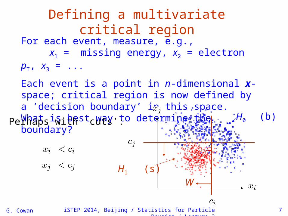
Defining a multivariate critical region
For each event, measure, e.g.,x1 = missing energy, x2 = electron pT, x3 = ...
Each event is a point in n-dimensional x-space; critical region is now defined by a ‘decision boundary’ in this space.What is best way to determine the boundary?
W
H1 (s)
H0 (b)Perhaps with ‘cuts’:

G. Cowan iSTEP 2014, Beijing / Statistics for Particle Physics / Lecture 2 8
Other multivariate decision boundariesOr maybe use some other sort of decision boundary:
WH1
H0
W
H1
H0
linear or nonlinear
Multivariate methods for finding optimal critical region havebecome a Big Industry (neural networks, boosted decision trees,...).

G. Cowan iSTEP 2014, Beijing / Statistics for Particle Physics / Lecture 2 9
Test statisticsThe boundary of the critical region for an n-dimensional dataspace x = (x1,..., xn) can be defined by an equation of the form
We can work out the pdfs
Decision boundary is now a single ‘cut’ on t, defining the critical region.
So for an n-dimensional problem we have a corresponding 1-d problem.
where t(x1,…, xn) is a scalar test statistic.

iSTEP 2014, Beijing / Statistics for Particle Physics / Lecture 2 10
Test statistic based on likelihood ratio How can we choose a test’s critical region in an ‘optimal way’?
Neyman-Pearson lemma states:
To get the highest power for a given significance level in a test ofH0, (background) versus H1, (signal) the critical region should have
inside the region, and ≤ c outside, where c is a constant chosento give a test of the desired size.
Equivalently, optimal scalar test statistic is
N.B. any monotonic function of this is leads to the same test.G. Cowan

G. Cowan iSTEP 2014, Beijing / Statistics for Particle Physics / Lecture 2 11
Classification viewed as a statistical test
Probability to reject H0 if true (type I error):
α = size of test, significance level, false discovery rate
Probability to accept H0 if H1 true (type II error):
β = power of test with respect to H1
Equivalently if e.g. H0 = background, H1 = signal, use efficiencies:
G. Cowan iSTEP 2014, Beijing / Statistics for Particle Physics / Lecture 2 12
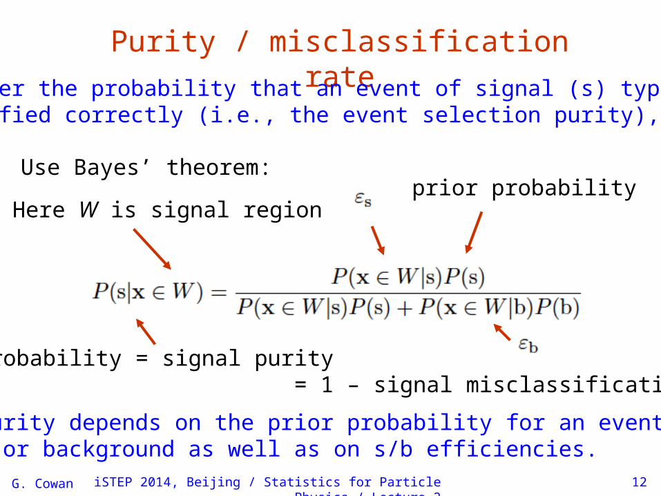
Purity / misclassification rate
Consider the probability that an event of signal (s) typeclassified correctly (i.e., the event selection purity),
Use Bayes’ theorem:
Here W is signal regionprior probability
posterior probability = signal purity = 1 – signal misclassification rate
Note purity depends on the prior probability for an event to besignal or background as well as on s/b efficiencies.

G. Cowan iSTEP 2014, Beijing / Statistics for Particle Physics / Lecture 2 13
Neyman-Pearson doesn’t usually help
We usually don’t have explicit formulae for the pdfs f (x|s), f (x|b), so for a given x we can’t evaluate the likelihood ratio
Instead we may have Monte Carlo models for signal and background processes, so we can produce simulated data:
generate x ~ f (x|s) → x1,..., xN
generate x ~ f (x|b) → x1,..., xN
This gives samples of “training data” with events of known type.
Can be expensive (1 fully simulated LHC event ~ 1 CPU minute).

G. Cowan iSTEP 2014, Beijing / Statistics for Particle Physics / Lecture 2 14
Approximate LR from histogramsWant t(x) = f (x|s)/ f(x|b) for x here
N (x|s) ≈ f (x|s)
N (x|b) ≈ f (x|b)
N(x|s)
N(x|b)
One possibility is to generateMC data and constructhistograms for bothsignal and background.
Use (normalized) histogram values to approximate LR:
x
x
Can work well for single variable.

G. Cowan iSTEP 2014, Beijing / Statistics for Particle Physics / Lecture 2 15
Approximate LR from 2D-histogramsSuppose problem has 2 variables. Try using 2-D histograms:
Approximate pdfs using N (x,y|s), N (x,y|b) in corresponding cells.
But if we want M bins for each variable, then in n-dimensions wehave Mn cells; can’t generate enough training data to populate.
→ Histogram method usually not usable for n > 1 dimension.
signal back-ground

G. Cowan iSTEP 2014, Beijing / Statistics for Particle Physics / Lecture 2 16
Strategies for multivariate analysis
Neyman-Pearson lemma gives optimal answer, but cannot beused directly, because we usually don’t have f (x|s), f (x|b).
Histogram method with M bins for n variables requires thatwe estimate Mn parameters (the values of the pdfs in each cell),so this is rarely practical.
A compromise solution is to assume a certain functional formfor the test statistic t (x) with fewer parameters; determine them(using MC) to give best separation between signal and background.
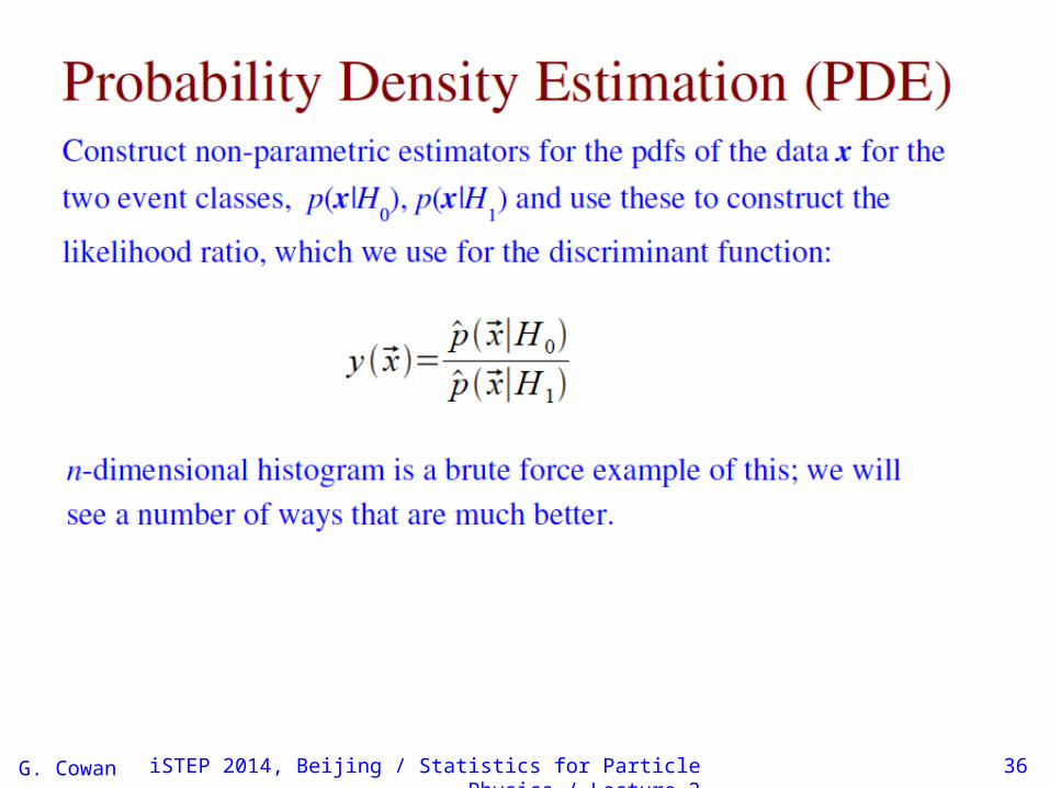
Alternatively, try to estimate the probability densities f (x|s) and f (x|b) (with something better than histograms) and use the estimated pdfs to construct an approximate likelihood ratio.

G. Cowan iSTEP 2014, Beijing / Statistics for Particle Physics / Lecture 2 17
Linear test statistic
Suppose there are n input variables: x = (x1,..., xn).
Consider a linear function:
For a given choice of the coefficients w = (w1,..., wn) we willget pdfs f (y|s) and f (y|b) :

G. Cowan iSTEP 2014, Beijing / Statistics for Particle Physics / Lecture 2 18
Linear test statistic
Fisher: to get large difference between means and small widths for f (y|s) and f (y|b), maximize the difference squared of theexpectation values divided by the sum of the variances:
Setting ∂J / ∂wi = 0 gives:
,
G. Cowan iSTEP 2014, Beijing / Statistics for Particle Physics / Lecture 2 19
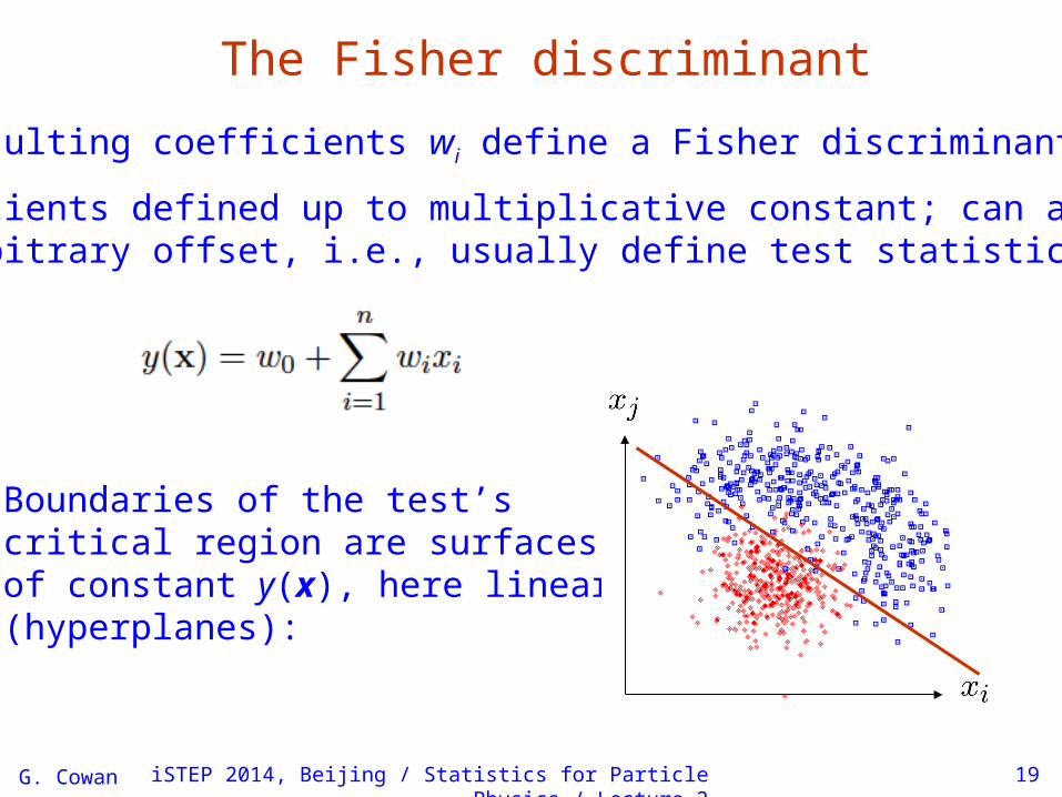
The Fisher discriminant
The resulting coefficients wi define a Fisher discriminant.
Coefficients defined up to multiplicative constant; can alsoadd arbitrary offset, i.e., usually define test statistic as
Boundaries of the test’scritical region are surfaces of constant y(x), here linear (hyperplanes):

G. Cowan iSTEP 2014, Beijing / Statistics for Particle Physics / Lecture 2 20
Fisher discriminant for Gaussian data
Suppose the pdfs of the input variables, f (x|s) and f (x|b), are both multivariate Gaussians with same covariance but different means:
f (x|s) = Gauss(μs, V)
f (x|b) = Gauss(μb, V)
Same covariance Vij = cov[xi, xj]
In this case it can be shown that the Fisher discriminant is
i.e., it is a monotonic function of the likelihood ratio and thusleads to the same critical region. So in this case the Fisherdiscriminant provides an optimal statistical test.

G. Cowan iSTEP 2014, Beijing / Statistics for Particle Physics / Lecture 2 21

G. Cowan iSTEP 2014, Beijing / Statistics for Particle Physics / Lecture 2 22
G. Cowan iSTEP 2014, Beijing / Statistics for Particle Physics / Lecture 2 23

G. Cowan iSTEP 2014, Beijing / Statistics for Particle Physics / Lecture 2 24

G. Cowan iSTEP 2014, Beijing / Statistics for Particle Physics / Lecture 2 25

G. Cowan iSTEP 2014, Beijing / Statistics for Particle Physics / Lecture 2 26
The activation functionFor activation function h(·) often use logistic sigmoid:

G. Cowan iSTEP 2014, Beijing / Statistics for Particle Physics / Lecture 2 27

G. Cowan iSTEP 2014, Beijing / Statistics for Particle Physics / Lecture 2 28

G. Cowan iSTEP 2014, Beijing / Statistics for Particle Physics / Lecture 2 29

G. Cowan iSTEP 2014, Beijing / Statistics for Particle Physics / Lecture 2 30
G. Cowan iSTEP 2014, Beijing / Statistics for Particle Physics / Lecture 2 31
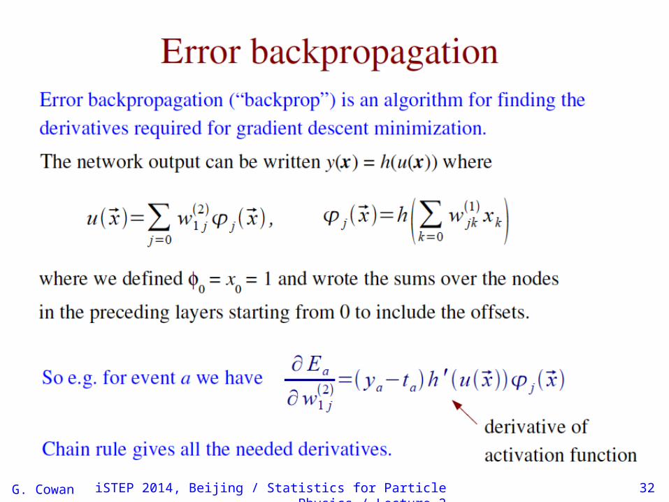
G. Cowan iSTEP 2014, Beijing / Statistics for Particle Physics / Lecture 2 32

G. Cowan iSTEP 2014, Beijing / Statistics for Particle Physics / Lecture 2 33
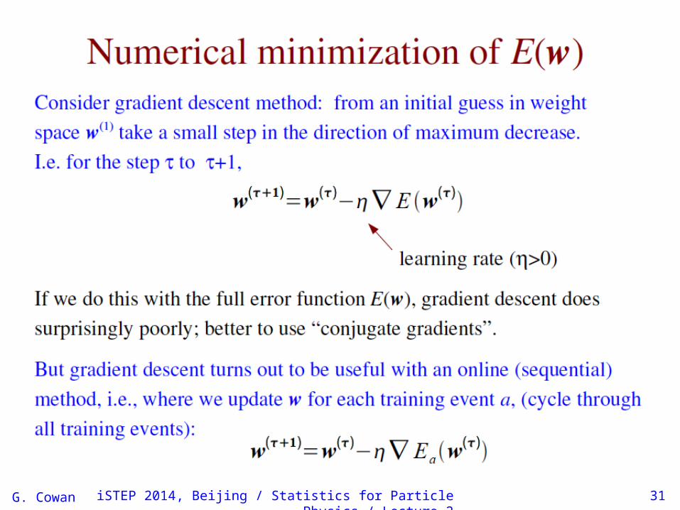
OvertrainingIncluding more parameters in a classifier makes its decision boundary increasingly flexible, e.g., more nodes/layers for a neural network.
A “flexible” classifier may conform too closely to the training points; the same boundary will not perform well on an independent test data sample (→ “overtraining”).
training sample independent test sample
G. Cowan iSTEP 2014, Beijing / Statistics for Particle Physics / Lecture 2 34
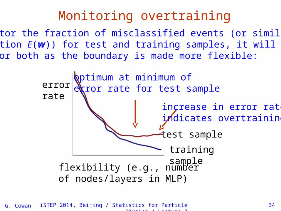
Monitoring overtrainingIf we monitor the fraction of misclassified events (or similar, e.g., error function E(w)) for test and training samples, it will usually decrease for both as the boundary is made more flexible:
errorrate
flexibility (e.g., number of nodes/layers in MLP)
test sample
training sample
optimum at minimum oferror rate for test sample
increase in error rateindicates overtraining

G. Cowan iSTEP 2014, Beijing / Statistics for Particle Physics / Lecture 2 page 35
Neural network example from LEP IISignal: ee → WW (often 4 well separated hadron jets)
Background: ee → qqgg (4 less well separated hadron jets)
← input variables based on jetstructure, event shape, ...none by itself gives much separation.
Neural network output:
(Garrido, Juste and Martinez, ALEPH 96-144)
G. Cowan iSTEP 2014, Beijing / Statistics for Particle Physics / Lecture 2 36

G. Cowan iSTEP 2014, Beijing / Statistics for Particle Physics / Lecture 2 37

G. Cowan iSTEP 2014, Beijing / Statistics for Particle Physics / Lecture 2 38

G. Cowan iSTEP 2014, Beijing / Statistics for Particle Physics / Lecture 2 39

G. Cowan iSTEP 2014, Beijing / Statistics for Particle Physics / Lecture 2 40
Naive Bayes methodIf the nonlinear features are not too important, it is reasonable to first decorrelate the input variables and estimate f (x) with
⌃where fi(xi) is an estimate of the one-dimensional marginal pdf of the ith variable (after decorrelation).
Do this separately for both pdfs (signal and background); resultingratio gives “Naive Bayes” classifier (in HEP sometimes called“likelihood method”).
This reduces the problem of estimating an n-dimensional pdf tothat of finding n one-dimensional pdfs.

G. Cowan iSTEP 2014, Beijing / Statistics for Particle Physics / Lecture 2 41
Kernel-based PDE (KDE)Consider d dimensions, N training events, x1, ..., xN, estimate f (x) with
Use e.g. Gaussian kernel:
kernelbandwidth (smoothing parameter)
x where we want to know pdf
x of ith trainingevent
G. Cowan iSTEP 2014, Beijing / Statistics for Particle Physics / Lecture 2 42
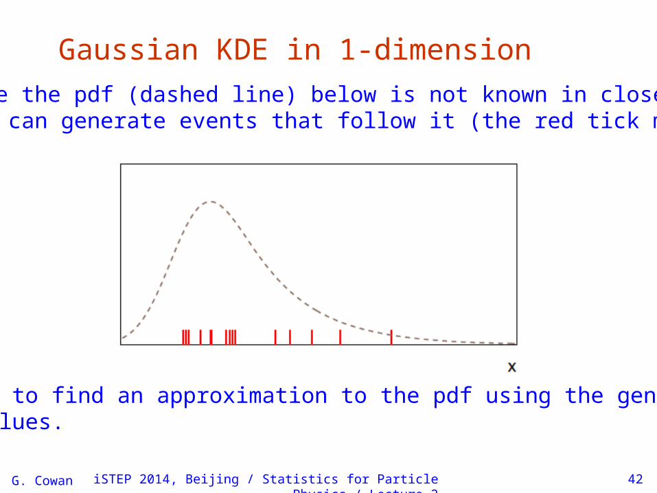
Gaussian KDE in 1-dimension
Suppose the pdf (dashed line) below is not known in closed form, but we can generate events that follow it (the red tick marks):
Goal is to find an approximation to the pdf using the generated date values.

G. Cowan iSTEP 2014, Beijing / Statistics for Particle Physics / Lecture 2 43
Gaussian KDE in 1-dimension (cont.)
Place a kernel pdf (here a Gaussian) centred around each generated event weighted by 1/Nevent:

G. Cowan iSTEP 2014, Beijing / Statistics for Particle Physics / Lecture 2 44
Gaussian KDE in 1-dimension (cont.)
The KDE estimate the pdf is given by the sum of all of the Gaussians:

G. Cowan iSTEP 2014, Beijing / Statistics for Particle Physics / Lecture 2 45
Choice of kernel width
The width h of the Gaussians is analogous to the bin widthof a histogram. If it is too small, the estimator has noise:

G. Cowan iSTEP 2014, Beijing / Statistics for Particle Physics / Lecture 2 46
If width of Gaussian kernels too large, structure is washed out:
Choice of kernel width (cont.)

G. Cowan iSTEP 2014, Beijing / Statistics for Particle Physics / Lecture 2 47
Various strategies can be applied to choose width h of kernelbased trade-off between bias and variance (noise).
Adaptive KDE allows width of kernel to vary, e.g., wide wheretarget pdf is low (few events); narrow where pdf is high.
Advantage of KDE: no training!
Disadvantage of KDE: to evaluate we need to sum Nevent terms, so if we have many events this can be slow.
Special treatment required if kernel extends beyond rangewhere pdf defined. Can e.g., renormalize the kernels to unityinside the allowed range; alternatively “mirror” the eventsabout the boundary (contribution from the mirrored events exactly compensates the amount lost outside the boundary).
Software in ROOT: RooKeysPdf (K. Cranmer, CPC 136:198,2001)
KDE discussion

G. Cowan iSTEP 2014, Beijing / Statistics for Particle Physics / Lecture 2 48
Each event characterized by 3 variables, x, y, z:

G. Cowan iSTEP 2014, Beijing / Statistics for Particle Physics / Lecture 2 49
Test example (x, y, z)
no cut on z
z < 0.5 z < 0.25
z < 0.75
x
xx
x
y
y
y
y

G. Cowan iSTEP 2014, Beijing / Statistics for Particle Physics / Lecture 2 50
Test example results
Fisherdiscriminant
Naive Bayes, no decor-relation
Multilayerperceptron
Naive Bayeswith decor-relation

G. Cowan iSTEP 2014, Beijing / Statistics for Particle Physics / Lecture 2 page 51
Particle i.d. in MiniBooNEDetector is a 12-m diameter tank of mineral oil exposed to a beam of neutrinos and viewed by 1520 photomultiplier tubes:
H.J. Yang, MiniBooNE PID, DNP06H.J. Yang, MiniBooNE PID, DNP06
Search for to e oscillations
required particle i.d. using information from the PMTs.

G. Cowan iSTEP 2014, Beijing / Statistics for Particle Physics / Lecture 2 page 52
Decision treesOut of all the input variables, find the one for which with a single cut gives best improvement in signal purity:
Example by MiniBooNE experiment,B. Roe et al., NIM 543 (2005) 577
where wi. is the weight of the ith event.
Resulting nodes classified as either signal/background.
Iterate until stop criterion reached based on e.g. purity or minimum number of events in a node.
The set of cuts defines the decision boundary.
G. Cowan iSTEP 2014, Beijing / Statistics for Particle Physics / Lecture 2 page 53
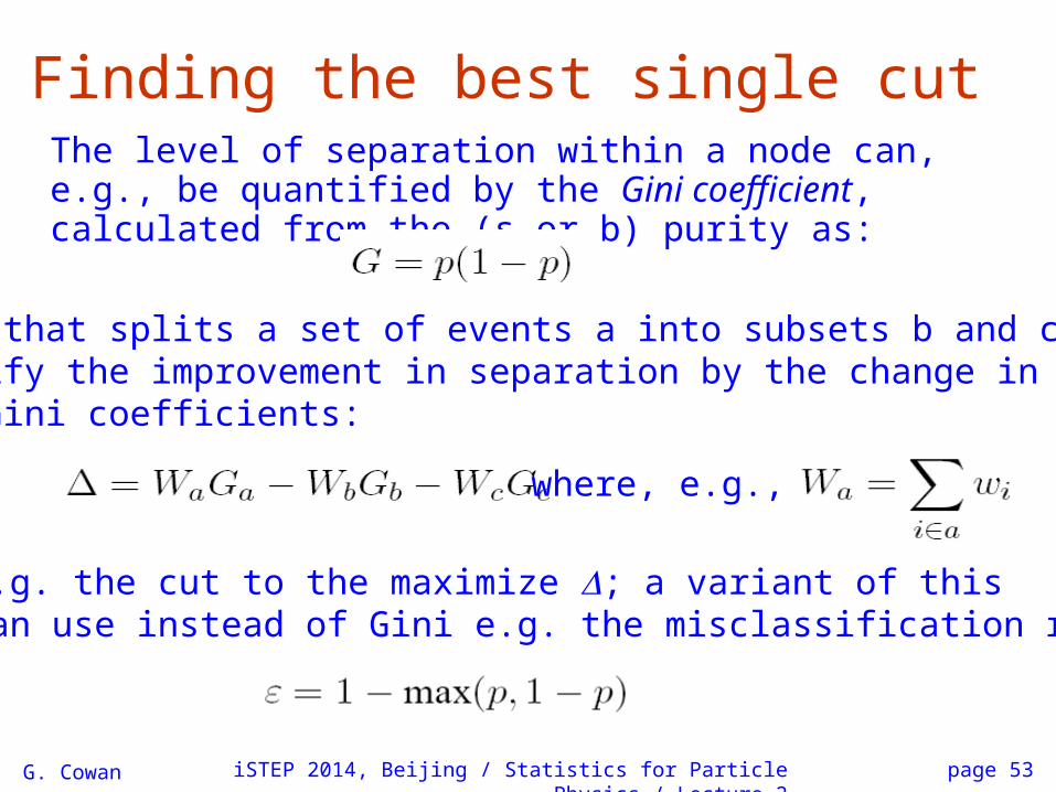
Finding the best single cutThe level of separation within a node can, e.g., be quantified by the Gini coefficient, calculated from the (s or b) purity as:
For a cut that splits a set of events a into subsets b and c, onecan quantify the improvement in separation by the change in weighted Gini coefficients:
where, e.g.,
Choose e.g. the cut to the maximize ; a variant of thisscheme can use instead of Gini e.g. the misclassification rate:
G. Cowan iSTEP 2014, Beijing / Statistics for Particle Physics / Lecture 2 page 54
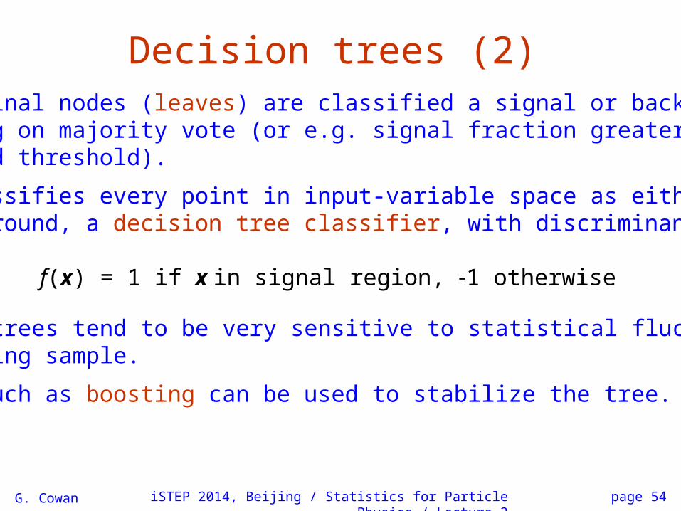
Decision trees (2)The terminal nodes (leaves) are classified a signal or backgrounddepending on majority vote (or e.g. signal fraction greater than aspecified threshold).
This classifies every point in input-variable space as either signalor background, a decision tree classifier, with discriminant function
f(x) = 1 if x in signal region, 1 otherwise
Decision trees tend to be very sensitive to statistical fluctuations inthe training sample.
Methods such as boosting can be used to stabilize the tree.
G. Cowan iSTEP 2014, Beijing / Statistics for Particle Physics / Lecture 2 page 55

G. Cowan iSTEP 2014, Beijing / Statistics for Particle Physics / Lecture 2 page 56
1
1

G. Cowan iSTEP 2014, Beijing / Statistics for Particle Physics / Lecture 2 page 57
G. Cowan iSTEP 2014, Beijing / Statistics for Particle Physics / Lecture 2 page 58

G. Cowan iSTEP 2014, Beijing / Statistics for Particle Physics / Lecture 2 page 59
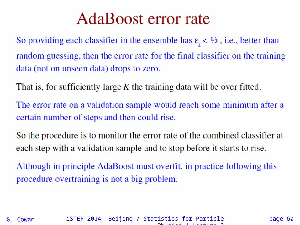
G. Cowan iSTEP 2014, Beijing / Statistics for Particle Physics / Lecture 2 page 60
<
G. Cowan iSTEP 2014, Beijing / Statistics for Particle Physics / Lecture 2 page 61

G. Cowan iSTEP 2014, Beijing / Statistics for Particle Physics / Lecture 2 page 62
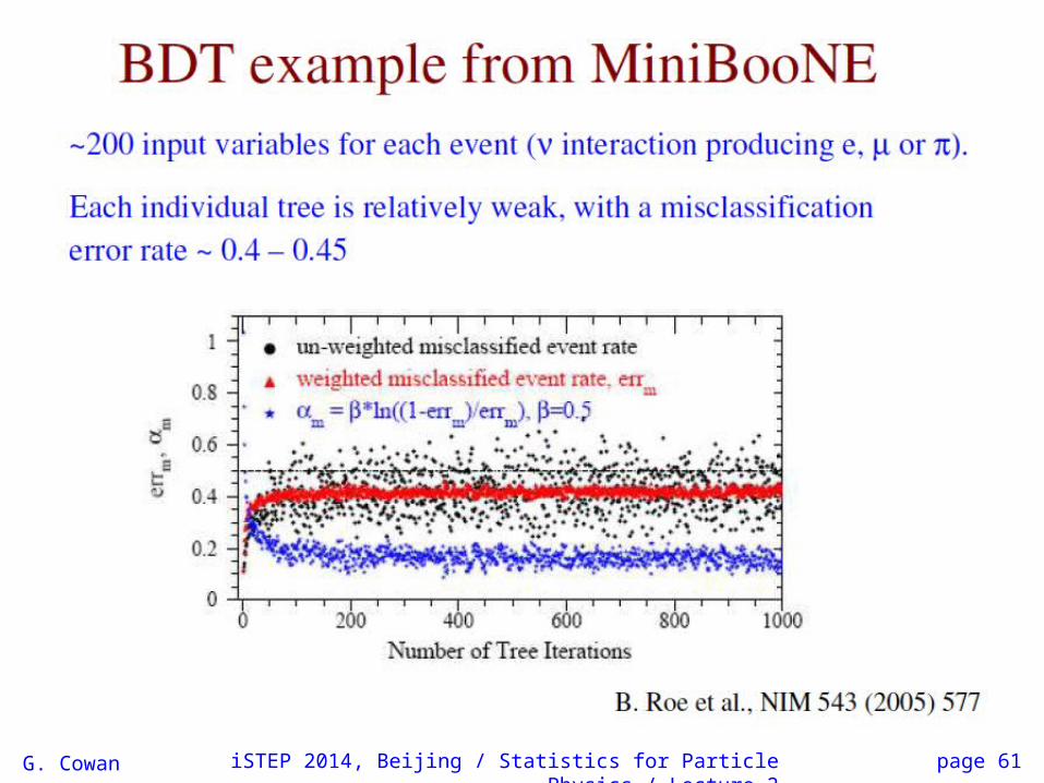
Monitoring overtraining
From MiniBooNEexample:
Performance stableafter a few hundredtrees.

G. Cowan iSTEP 2014, Beijing / Statistics for Particle Physics / Lecture 2 page 63
A simple example (2D)Consider two variables, x1 and x2, and suppose we have formulas for the joint pdfs for both signal (s) and background (b) events (in real problems the formulas are usually notavailable).
f(x1|x2) ~ Gaussian, different means for s/b, Gaussians have same σ, which depends on x2, f(x2) ~ exponential, same for both s and b, f(x1, x2) = f(x1|x2) f(x2):

G. Cowan iSTEP 2014, Beijing / Statistics for Particle Physics / Lecture 2 page 64
Joint and marginal distributions of x1, x2
background
signal
Distribution f(x2) same for s, b.
So does x2 help discriminatebetween the two event types?

G. Cowan iSTEP 2014, Beijing / Statistics for Particle Physics / Lecture 2 page 65
Likelihood ratio for 2D example
Neyman-Pearson lemma says best critical region is determinedby the likelihood ratio:
Equivalently we can use any monotonic function of this asa test statistic, e.g.,
Boundary of optimal critical region will be curve of constant ln t, and this depends on x2!

G. Cowan iSTEP 2014, Beijing / Statistics for Particle Physics / Lecture 2 page 66
Contours of constant MVA output
Exact likelihood ratio Fisher discriminant

G. Cowan iSTEP 2014, Beijing / Statistics for Particle Physics / Lecture 2 page 67
Contours of constant MVA output
Multilayer Perceptron1 hidden layer with 2 nodes
Boosted Decision Tree200 iterations (AdaBoost)
Training samples: 105 signal and 105 background events

G. Cowan iSTEP 2014, Beijing / Statistics for Particle Physics / Lecture 2 page 68
ROC curve
ROC = “receiver operating characteristic” (term from signal processing).
Shows (usually) background rejection (1εb) versus signal efficiency εs.
Higher curve is better; usually analysis focused ona small part of the curve.

G. Cowan iSTEP 2014, Beijing / Statistics for Particle Physics / Lecture 2 page 69
2D Example: discussionEven though the distribution of x2 is same for signal and background, x1 and x2 are not independent, so using x2 as an input variable helps.
Here we can understand why: high values of x2 correspond to a smaller σ for the Gaussian of x1. So high x2 means that the value of x1 was well measured.
If we don’t consider x2, then all of the x1 measurements are lumped together. Those with large σ (low x2) “pollute” the well measured events with low σ (high x2).
Often in HEP there may be variables that are characteristic of how well measured an event is (region of detector, number of pile-up vertices,...). Including these variables in a multivariate analysis preserves the information carried by the well-measured events, leading to improved performance.
In this example we can understand why x2 is useful, eventhough both signal and background have same pdf for x2.

G. Cowan iSTEP 2014, Beijing / Statistics for Particle Physics / Lecture 2 page 70
Summary on multivariate methodsParticle physics has used several multivariate methods for many years:
linear (Fisher) discriminantneural networksnaive Bayes
and has in recent years started to use a few more:
boosted decision treessupport vector machineskernel density estimationk-nearest neighbour
The emphasis is often on controlling systematic uncertainties betweenthe modeled training data and Nature to avoid false discovery.
Although many classifier outputs are "black boxes", a discoveryat 5 significance with a sophisticated (opaque) method will win thecompetition if backed up by, say, 4 evidence from a cut-based method.

G. Cowan iSTEP 2014, Beijing / Statistics for Particle Physics / Lecture 2 page 71
Extra slides
G. Cowan iSTEP 2014, Beijing / Statistics for Particle Physics / Lecture 2 72
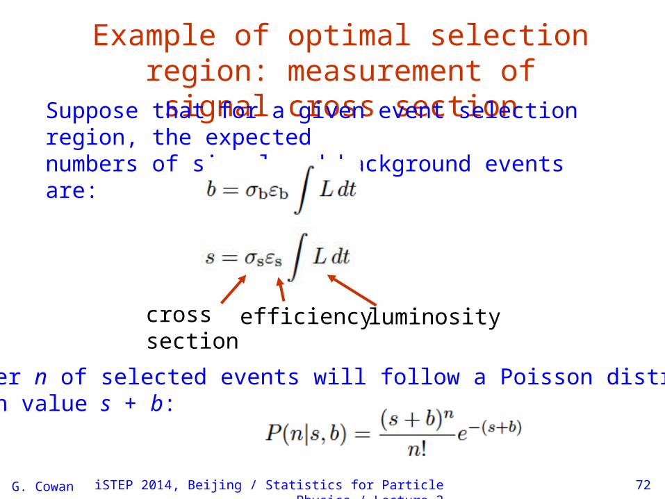
Example of optimal selection region: measurement of signal cross section
Suppose that for a given event selection region, the expectednumbers of signal and background events are:
cross section
efficiency luminosity
The number n of selected events will follow a Poisson distribution with mean value s + b:

G. Cowan iSTEP 2014, Beijing / Statistics for Particle Physics / Lecture 2 73
Optimal selection for measurement of signal rateSuppose only unknown is s (or equivalently, σs) and goal is tomeasure this with best possible accuracy by counting the numberof events n observed in data. The (log-)likelihood function is
Set derivative of lnL(s) with respect to s equal to zero and solveto find maximum-likelihood estimator:
Variance of s is:⌃
So “relative precision” of measurement is:

G. Cowan iSTEP 2014, Beijing / Statistics for Particle Physics / Lecture 2 74
Optimal selection (continued)So if our goal is best relative precision of a measurement, then choose the event selection region to maximize
In other analyses, we may not know whether the signalprocess exists (e.g., SUSY), and goal is to search for it.
Then we try to maximize the probability, assuming the signal exists, of discovery, i.e., rejecting background-only hypothesis.
To do this we can maximize, e.g.,
or similar (depending on details of problem; more on this later).
In general, optimal trade-off between efficiency and puritywill depend on the goals of the analysis.


![Multivariate Methods Nutshell [Read-Only]ww2.chemistry.gatech.edu/class/6282/janata/Multivariate... · 2003-11-26 · Chemometrics The secrets behind multivariate methods in a nutshell!](https://static.fdocuments.net/doc/165x107/5f84ce108c82b03184669661/multivariate-methods-nutshell-read-onlyww2-2003-11-26-chemometrics-the-secrets.jpg)